Atmospheric Boundary Layer and Tropopause Retrievals from FY-3/GNOS-II Radio Occultation Profiles

Abstract

The atmospheric boundary layer (ABL) and tropopause play critical roles in weather formation and climate change. This study initially focuses on the ABL height (ABLH), tropopause height (TPH), and temperature (TPT) retrieved from the integrated radio occultation (RO) profiles from FY-3E, FY-3F, and FY-3G satellites during September 2022 to August 2024. All three FY-3 series satellites are equipped with the RO payload of Global Navigation Satellite System Radio Occultation Sounder-II (GNOS-II), which includes open-loop tracking RO observations from the BeiDou navigation satellite system (BDS) and the Global Positioning System (GPS). The wavelet covariance transform method was used to determine the ABL top, and the temperature lapse rate was applied to judge the tropopause. Results show that the maximum ABL detection rate of FY-3/GNOS-II RO can reach up to 76% in the subtropical eastern Pacific, southern hemisphere Atlantic, and eastern Indian Ocean. The ABLH is highly consistent with the collocated radiosonde observations and presents distinct seasonal variations. The TPH retrieved from FY-3/GNOS-II RO profiles is in agreement with the radiosonde-derived TPH, and both TPH and TPT from RO profiles display well-defined spatial structures. From 45°S to 45°N and south of 55°S, the annual cycle of the TPT is negatively correlated with the TPH. This study substantiates the promising performance of FY-3/GNOS-II RO measurements in observing the ABL and tropopause, which can be incorporated into the weather and climate systems.

1. Introduction

As the lowest layer of the Earth’s troposphere and the transition layer from the troposphere to the stratosphere, the atmospheric boundary layer (ABL), also known as the planetary boundary layer (PBL), and the tropopause are both important components of the Earth’s atmosphere. The ABL exchanges energy between the Earth’s surface and the free troposphere, where turbulent processes typically dominate the vertical redistribution of heat, momentum, moisture, and aerosols [1]. The height of ABL (ABLH) is defined as the altitude from the Earth’s surface to the top of ABL. The ABLH serves as an essential parameter that holistically characterizes its dynamic features while exhibiting strong correlations with key variables in climatology and meteorology [2,3]. The ABLH spatiotemporal variation research can help to better understand the transport processes in the lower troposphere [4]. The tropopause plays a crucial role in dynamical variability and the trace gas exchange within the transition regions [5]. Research of tropopause parameters is critical for understanding stratosphere–troposphere exchange [6,7].

Various methods can be used to study the ABL, including simulation using general circulation models (GCMs) [2], inversion using atmospheric reanalysis datasets [3], radiosonde data [8], and ground-based remote sensing, and in situ instrument observations [9,10]. Satellite-based observations were also widely used, including lidar measurements [11], temperature, and water vapor profiles provided by the Atmospheric Infrared Sounder (AIRS) [12], and Moderate Resolution Imaging Spectroradiometer (MODIS) and Tropical Rainfall Measuring Mission (TRMM) Microwave Imager (TMI) observations for inversion of the ABLH [13]. The main data sources for the study of tropopause parameters are reanalysis and radiosonde data [14,15]. Some early literature used the GCM model to study the sensitivity of tropopause height (TPH) to various external parameters [16,17]. And the satellite-based lidar was also dedicated to studying clouds and aerosols at the tropopause [18].

Here, a spaceborne remote sensing technique listed separately is the Global Navigation Satellite System (GNSS) Radio Occultation (RO). GNSS RO is a limb-sounding technique that allows for the Earth’s atmospheric profiling by inverting the bending and delay effects of GNSS satellites’ signals traversing the atmosphere to low Earth orbit receivers [19,20]. GNSS RO has the advantages of global coverage and full diurnal cycle of sampling, high vertical resolution, and insensitivity to clouds and precipitation [21]. Moreover, RO observations are long-term stable since they are calibration-free [22], and RO enables all-weather sampling. Therefore, RO is a well-suited technique for monitoring the vertical structure and height of the ABL and tropopause. However, early use of GNSS RO for ABL determination was limited by the closed-loop (CL) tracking [23]. Because in the moist lower troposphere, the difficulty of CL tracking can lead to loss of lock or biases in phase, and make the value of retrieved refractivity missing [24,25]. The open-loop (OL) tracking technology does not rely on real-time signal feedback and tracks the RO signal directly based on a preset model [24]. Compared to the CL, the OL is able to maintain stable tracking even in a low signal-to-noise ratio during the initial phase of rising occultations. The OL technology compensates for the problem of missing data from the CL in the lower atmosphere, improving the integrity of vertical profiles and the quality of low-level data. Benefiting from the OL that allows RO to produce complete, high-quality observations in the lower troposphere, RO data can be better and widely utilized to study the ABL from various missions [26,27,28,29,30,31,32,33]. Applying the OL can also increase the proportion of RO profiles that can observe the tropopause, especially in polar regions where the tropopause is very low. The results from He et al. (2023) show that the OL tracking improved the percentage of BeiDou navigation satellite system (BDS) occultations capable of penetrating 8–12 km by more than 20% [34]. With either CL or OL tracking, RO data were also used to study the structures, spatiotemporal variations, climate characteristics, and detection methods of the tropopause [7,35,36,37,38,39].

The FengYun-3 (FY-3) series are China’s second-generation polar-orbiting meteorological satellites. Since the launch of the FY-3C satellite in 2013, the FY-3 series has been equipped with the RO payload of Global Navigation Satellite System Radio Occultation Sounder (GNOS). Recently, studies on the application of FY-3 series RO data to the ABL and tropopause have stalled at FY-3C [31,38,39,40]. Zhu et al. (2021) validated the feasibility of using FY-3C RO data to detect the ABL [31]. However, the refractivity product published by the National Satellite Meteorological Center (NSMC) did not include BDS RO profiles, and only a brief analysis of the annual ABLH results was provided. Liu et al. (2019) preliminarily validated the application of FY-3C RO data in the thermal tropopause [38]. Liu et al. (2021) and Li et al. (2021) compared different methods for detecting tropopause [39,40]. The upgraded GNOS-II RO payload on the latest FY-3 series satellites could track the OL BDS-2 and BDS-3 RO signals, significantly enhancing the penetration depth of BDS RO events [34]. The abundance of BDS and GPS (Global Positioning System) RO data from FY-3/GNOS-II can also allow for more detailed analysis for ABL and tropopause studies. Therefore, this study incorporates newly released RO datasets from the FY-3 satellites carrying the GNOS-II, including FY-3E, FY-3F, and FY-3G, for the period September 2022 to August 2024 to derive the global ABLH, TPH, and tropopause temperature (TPT). Based on two years of RO profiles, the spatial structures, seasonal cycles, and annual variations in the ABLH, TPH, and TPT were analyzed.

The present study is organized as follows: after this Section 1, the datasets used in this research are specified in Section 2. Section 3 describes the methods for extracting the ABLH and tropopause parameters. The ABLH and TPH, respectively derived from FY-3/GNOS-II RO profiles and collocated radiosonde measurements, are compared in Section 4. In Section 5, the analysis results of the ABL and tropopause are described in detail in two separate subsections. Section 6 discusses the results. The final Section 7 summarizes and concludes this study.

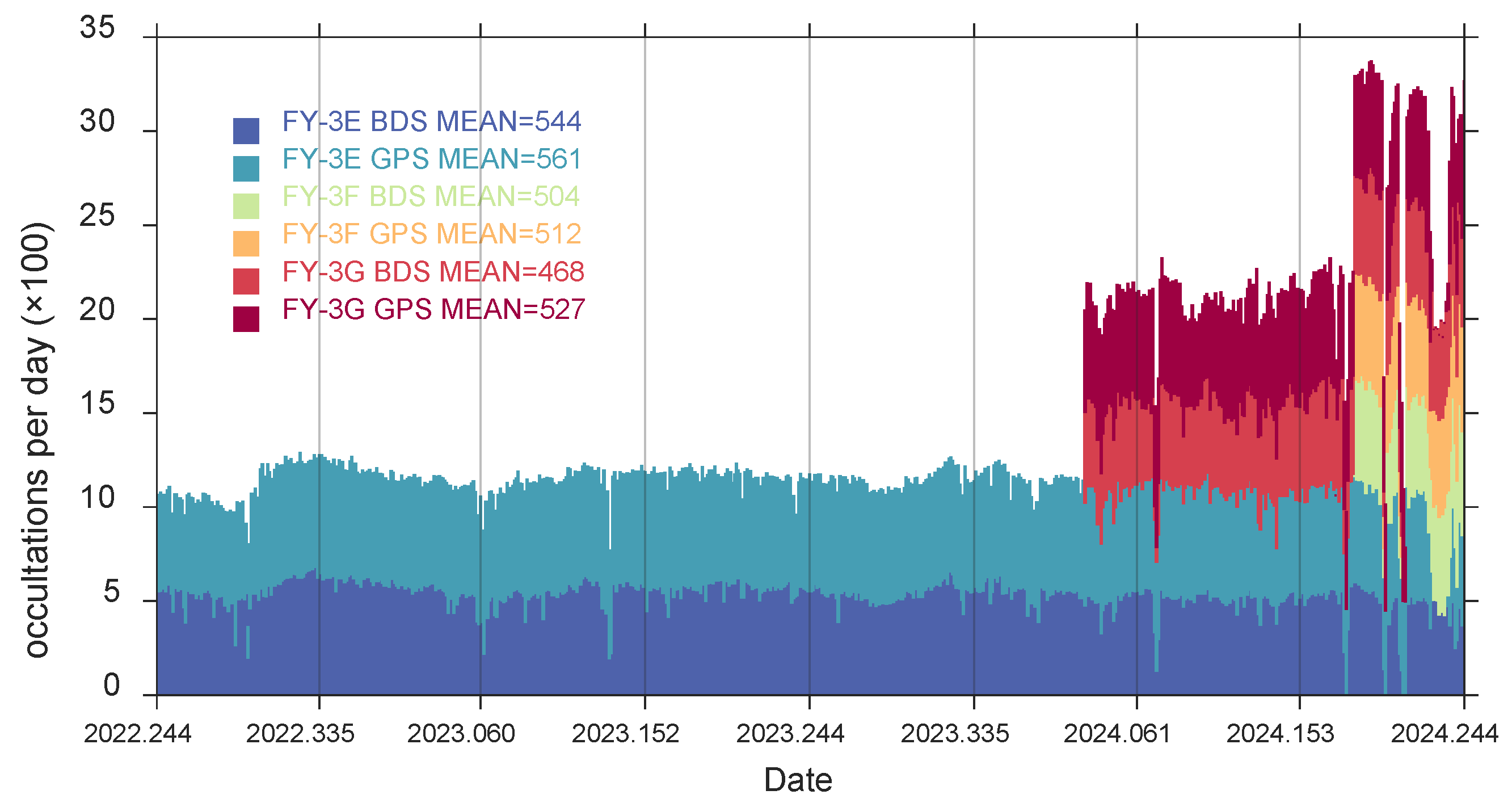
2. FY-3/GNOS-II RO Observations, Radiosonde, and Other Ancillary Data

The RO data used in this study are from the third batch of FY-3 satellites, as shown in

Table 1. Overview of the RO missions and selected data period from the FY-3 satellites used in this study.

Mission	Launch Time	Orbital Inclination	Period (yyyy.doy)
FY-3E	5 July 2021	98.75°	2022.244–2024.244
FY-3F	3 August 2023	98.75°	2024.032–2024.244
FY-3G	16 April 2023	50° ± 1°	2024.183–2024.244

, including FY-3E, FY-3F, and FY-3G. FY-3E is the world’s first civilian early-morning orbiting meteorological satellite, which first released the publicly available products of BDS RO. The FY-3F satellite replaced the morning satellite FY-3C, whose RO payload had ceased operation in 2018, and the FY-3G is a low-inclination-orbit satellite. All three satellites carry the RO payload of GNOS-II, and detailed information about the instrument can be accessed from the research by Sun et al. (2017) [41].

In this research, the FY-3/GNOS-II RO profiles were downloaded from the NSMC (http://satellite.nsmc.org.cn, accessed on 2 September 2024). The refractivity, temperature, and pressure profiles are provided in the ATP (atmospheric temperature profile) file, which also contains necessary attribute information such as latitude and longitude, mean sea level (MSL) altitude, etc. The atmospheric parameters retrieval of FY-3 series satellite RO can be referred to the study of Liao et al. (2016) [42]. The accuracy of the atmospheric profiles retrieved from FY-3/GNOS-II RO has been verified. For example, compared with the National Centers for Environmental Prediction (NCEP) Final (FNL) global atmospheric analysis data, the mean difference and standard deviation of the FY-3E RO refractivity are less than 0.2% and 1% in 5–30 km, respectively, which is consistent with the accuracy level of FY-3D/GNOS RO data (Liu et al., 2023) [43]. Moreover, the accuracy and precision of FY-3E BDS and GPS RO profiles are comparable (He et al., 2023) [34]. The vertical resolution of FY-3/GNOS-II RO profiles for detecting the ABLH is 100–160 m in the altitude range of 0–5 km, and for detection, the TPH and TPT are 90–120 m in the altitude range of 5–25 km.

Figure 1 shows the daily number of RO events (ROEs) tracked from FY-3E, FY-3F, and FY-3G, respectively, which were obtained by continuous sampling throughout the day. The sessions of the RO data used are also listed in Table 1. Two years of FY-3E BDS and GPS (Global Positioning System) ROEs were used from 1 September 2022 to 31 August 2024. FY-3F and FY-3G have relatively limited data because they were launched later and tested in orbit for several months. Figure 1 shows that FY-3E could track over 1100 BDS and GPS occultations daily, and FY-3F and FY-3G tracked about 1000 ROEs. There are a total of 1,066,777 ROEs used in this study, including 522,289 BDS and 544,488 GPS ROEs.

Figure 2 shows the spatial coverage of the FY-3/GNOS-II ROEs at every 2.5° latitude in July 2024. FY-3E and FY-3F ROEs have global coverage. Due to the low orbital inclination of the FY-3G (as shown in Table 1), its ROEs cover a range of 65°N–65°S. The spatial coverages of the BDS and GPS ROEs are consistent with each other, with slight differences in latitude variations. All three satellites show more occultations in the mid latitudes around 20–50° on both northern (NH) and southern hemispheres (SH). The ROEs are relatively rare in both tropical and polar regions, and the smallest number of occultations in polar regions is attributed to the smallest area at the same latitudinal interval.

The radiosonde observations in this study were sourced from the Integrated Global Radiosonde Archive (IGRA, https://www.ncei.noaa.gov/products/weather-balloon/integrated-global-radiosonde-archive, accessed on 5 September 2024), which consists of the radiosonde and pilot balloon observations from globally distributed stations. The radiosonde data come from 759 stations worldwide, and these stations are mainly distributed in land and mid-latitude regions of the NH. Due to the uneven spatial distribution of radiosonde data, it is difficult to capture global or regional ABLH characteristics. The radiosonde data are usually observed at 0000 UTC and 1200 UTC daily. This low temporal resolution makes it challenging to consistently observe rapid variations in the ABL. In addition, some radiosondes terminate their observations in the lower stratosphere, which may result in the loss of complete tropopause information. For example, the TPH in tropical regions can reach 16–18 km. The quality of radiosonde observations is uneven, and data with a vertical resolution of about 80–160 m in 0–20 km were chosen as the reference in this study. For comparison with RO data, we selected derived parameters from the IGRA data, including variables of reported pressure, geopotential height, temperature, and refractive index.

Furthermore, the time-independent surface altitude from the sixth phase of the Coupled Model Intercomparison Project (CMIP6) model was used when calculating the ABLH [44]. The land-sea mask from the fifth-generation European Centre for Medium Range Weather Forecasts (ECMWF) reanalysis (ERA5) was used to separate land from ocean regions [45]. These data are all available through the Climate Data Store (CDS, cds.climate.copernicus.eu/cdsapp#!/home, accessed on 5 August 2024) maintained by ECMWF.

3. Methods to Retrieve ABLH, TPH, and TPT

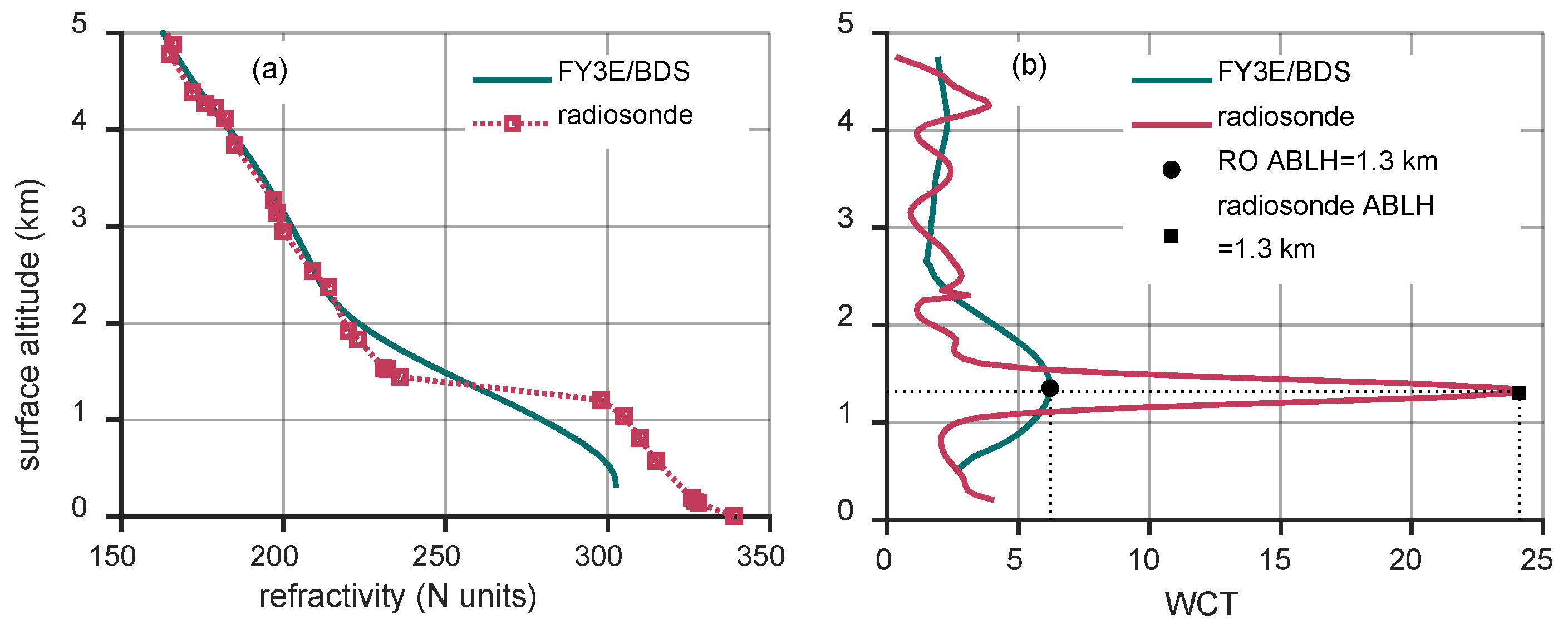
3.1. ABLH Estimation with WCT Method

The ABLH can be directly determined by the height corresponding to the minimum gradient of refractivity, temperature, or humidity profiles [3,21]. The vertical gradient method is simple and fast, very suitable for the case where the ABLH of the profile is dominated by a single strong inversion. However, when the inversion caused by ABL in the profile is weak, a more robust wavelet covariance transform (WCT) method was proposed [46]. Essentially, the WCT method involves sliding a window through the profile and locating the center of the window that produces the maximum step, which is considered the ABLH.

The WCT method is based on a compound step function Haar ($h$), which is defined as follows:

$$h\left({\displaystyle \frac{z-b}{a}}\right)=\left\{\begin{array}{c}+1, b-{\displaystyle \frac{a}{2}}\le z<b\\ -1, b\le z<b+{\displaystyle \frac{a}{2}}\\ 0, other \end{array}\right.$$

(1)

here $z$ is the height of the refractivity profile, $b$ is the center of the Haar function, and $a$ is the dilation parameter. The covariance transform of the Haar function is defined as $W_f$:

$$W_f\left(a,b\right)={\displaystyle \frac{1}{a}}\underset{z0}{\overset{z1}{\int }}f\left(z\right)h\left({\displaystyle \frac{z-b}{a}}\right)dz$$

(2)

where $f\left(z\right)$ is the analyzed refractivity profile. $z0$ and $z1$ are the lower and upper height limits used for integration. When $b=b_0$, we can calculate a value of $W_f\left(a,b_0\right)$, and when $W_f\left(a,b_0\right)$ is maximized on a profile, the corresponding $b_0$ is the ABLH we need. Theoretically, $a$ should be equal to the depth of the transition zone between the ABL and the free troposphere [47], but it is unknown, and its value needs to be determined through specific experiments [46]. In this study, taking $a$ = 0.4 km to detect the ABL top is optimal according to multiple calculations of the ABLH results and comparisons. Consistent with the value of $a$ in the research of Xu et al. (2018) [48], adopting this value does not lose excessive details of the profiles and is also applicable to most GNOS-II refractivity.

In addition, a quality parameter $\lambda$ is used to exclude data with weak feedback on ABL [31], and it could be calculated as:

$$\lambda =\left|{\displaystyle \frac{W_{max}}{RMS\left(W_f\right)}}\right|$$

(3)

where $W_{\mathrm{m}\mathrm{a}\mathrm{x}}$ is the maximum value of $W_f$. The $\lambda$ reflects the relative strength of the $W_f$. Larger $\lambda$ indicates that the step change in the profile is more obvious. For profiles with small $\lambda$ values less than 1.35, an empirical value obtained from the experiment, it is considered that the ABL cannot be identified. Compared to the research on FY-3C by Zhu et al. (2021) [31], larger $a$ and $\lambda$ values were used in the present study.

3.2. Determining the Tropopause Through Temperature Lapse Rate

According to the definition of the tropopause by the World Meteorological Organization (WMO) in 1957, the criteria for judgment are as follows: the lowest altitude where the temperature lapse rate is less than or equal to 2 °C/km, and the average lapse rate within 2 km above this altitude does not exceed 2 °C/km. The tropopause obtained by this method is denoted as LRT. Dry temperature and dry pressure profiles are needed to determine the tropopause. The temperature lapse rate $\mathsf{\Gamma }\left(p\right)$ is transformed as follows [49]:

$$\mathsf{\Gamma }\left(p\right)=-{\displaystyle \frac{\partial T}{\partial h}}=-{\displaystyle \frac{\partial T}{\partial p}}{\displaystyle \frac{\partial p}{\partial h}}=-{\displaystyle \frac{\partial T}{\partial p^{\mathrm{k}}}}{\displaystyle \frac{{\partial p}^{\mathrm{k}}}{\partial p}}{\displaystyle \frac{\partial p}{\partial h}}$$

(4)

where $T$ is the temperature profile, $h$ is the altitude, and $p$ is the pressure profile. $\mathrm{k}=R_{dry}/C_p$, in which $R_{dry}$ is the dry atmospheric constant and $C_p$ is the specific heat capacity of air under constant pressure conditions. Using the relationship between dry temperature and pressure in hydrostatic approximation and the gas equation transforms Equations (4) and (5):

$$\mathsf{\Gamma }\left(p\right)={\displaystyle \frac{\partial T}{\partial p^{\mathrm{k}}}}{\displaystyle \frac{p^{\mathrm{k}}}{T}}\left({\displaystyle \frac{\mathrm{k}g}{R_{dry}}}\right)$$

(5)

where $g$ is the gravitational acceleration. The temperature lapse rate located at pressure position $i+1/2$ is calculated, with the assumption that $T$ varies linearly with $p^{\mathrm{k}}$. The $p_{i+1/2}^{\mathrm{k}}$ and ${\mathsf{\Gamma }}_{i+1/2}$ are given as [49]:

$$p_{i+1/2}^{\mathrm{k}}={\displaystyle \frac{p_i^{\mathrm{k}}+p_{i+1}^{\mathrm{k}}}{2}}$$

(6)

$${\mathsf{\Gamma }}_{i+1/2}={\displaystyle \frac{\left(T_{i+1}-T_i\right)}{\left(p_{i+1}^{\mathrm{k}}-p_i^{\mathrm{k}}\right)}}{\displaystyle \frac{\left(p_{i+1}^{\mathrm{k}}+p_i^{\mathrm{k}}\right)}{\left(T_{i+1}+T_i\right)}}\left({\displaystyle \frac{g}{C_p}}\right)$$

(7)

In accordance with the definition of TPH, we search for the lowest point located at $p_{j+1/2}^{\mathrm{k}}$ for which the lapse rate ${\mathsf{\Gamma }}_{j+1/2}$ is less than 2 °C/km, and then confirm that the average lapse rate in the 2 km height range upwards from that point is also less than 2 °C/km. The range of the query point in this process lies between 75 hPa and 550 hPa [49]. Subsequently, the tropopause pressure $p_{TP}$ is then calculated by linear interpolation between pressure levels $j-1/2$ and $j+1/2$:

$$p_{TP}^{\mathrm{k}}=p_{j-1/2}^{\mathrm{k}}+{\displaystyle \frac{p_{j+1/2}^{\mathrm{k}}-p_{j-1/2}^{\mathrm{k}}}{{\mathsf{\Gamma }}_{j+1/2}-{\mathsf{\Gamma }}_{j-1/2}}}(2-{\mathsf{\Gamma }}_{j-1/2})$$

(8)

With linear interpolation, the temperature and height of the tropopause are calculated. Finally, there are two screenings of the TPH and TPT. One is that the TPH cannot exceed the range defined by the following two equations [39]:

$$\left\{\begin{array}{c}TPH\ge 2.5\times \left(3+\mathrm{c}\mathrm{o}\mathrm{s}(2\times lat)\right)\\ TPH\le 2.5\times \left(7+\mathrm{c}\mathrm{o}\mathrm{s}(2\times lat)\right)\end{array}\right.$$

(9)

The other is to avoid unreasonable LRT altitudes over polar regions. TPT less than 203 K was removed with latitude greater than 70° both over NH and SH [7].

4. Comparison with Independent Radiosonde Data

To validate the ABLH and TPH retrieved from FY-3/GNOS-II ROEs, collocated radiosonde observations were selected based on matching criteria of ±2 h temporal and ±2° longitude and latitude spatial thresholds.

The first step in validating ABL was to ensure that the profiles could penetrate down to 0.5 km.

Table 2. Percentage of RO profiles reaching the surface altitude of 0.5 km for each RO mission.

Missions	BDS RO	GPS RO	Total
FY-3E	40%	55%	48%
FY-3F	45%	57%	51%
FY-3G	47%	55%	51%

shows the percentage of RO profiles reaching surface altitudes at 0.5 km. As illustrated, the proportions of FY-3E, FY-3F, and FY-3G BDS RO profiles reaching 0.5 km are 40%, 45%, and 47%, while the percentages of GPS RO profiles are 55%, 57%, and 55%, respectively. The penetration depth of FY-3/GNOS-II GPS occultations was slightly lower than the BDS occultations, and thus, a larger proportion of the GPS occultations was reserved for the ABL retrieval. Overall, 48%, 51%, and 51% of all FY-3E, FY-3F, and FY-3G RO profiles were able to reach down to 0.5 km, respectively.

Additionally, refractivity profiles with detected ABLH values greater than 3.5 km were not used. In this study, with the application of multiple stringent constraints described above, about 26% of FY-3/GNOS-II ROEs were ultimately employed to detect the ABL with a sharp top.

4.1. The ABLH Validation

Figure 3 shows an example of retrieving the ABLH from FY-3E/BDS RO and radiosonde refractivity profiles by the WCT method. In Figure 3a, the ABL inversion characteristic of the RO profile is not as pronounced as the radiosonde data. The apparent gradient change from the radiosonde profile allowed it to easily find the exact altitude of the ABL top. Figure 3b illustrates the covariance transforms of the RO and radiosonde refractivity. The sharp peak of the radiosonde $W_f$ profile at 1.3 km corresponded to the ABLH. A raised structure was also visible in the RO $W_f$ profile at the same altitude, which was relatively more obvious with respect to the $W_f$ values at other altitudes as well.

Correlations between FY-3E, FY-3F, and FY-3G RO and collocated radiosonde ABLH samples are displayed in Figure 4. Owing to the fact that FY-3F had RO profiles for merely two months within the study period, the sample size of ABLH derived from the matching with radiosonde data was correspondingly reduced. In general, the ABLH derived from GNOS-II RO soundings correlated well with radiosonde measurements, with correlation coefficients of 0.73, 0.73, and 0.75 for FY-3E, FY-3F, and FY-3G, respectively. The correlations are significantly improved compared to the first generation of GNOS results [31]. GNOS-II RO ABLH results calculated by the WCT method are slightly lower than the radiosonde-derived results, as illustrated in Figure 4, with mean biases of −0.15 km for FY-3E, −0.11 km for FY-3F, and −0.10 km for FY-3G. A possible reason is the proximity of certain stations to oceans, and the collocated RO profiles contain ABL information of nearby oceans.

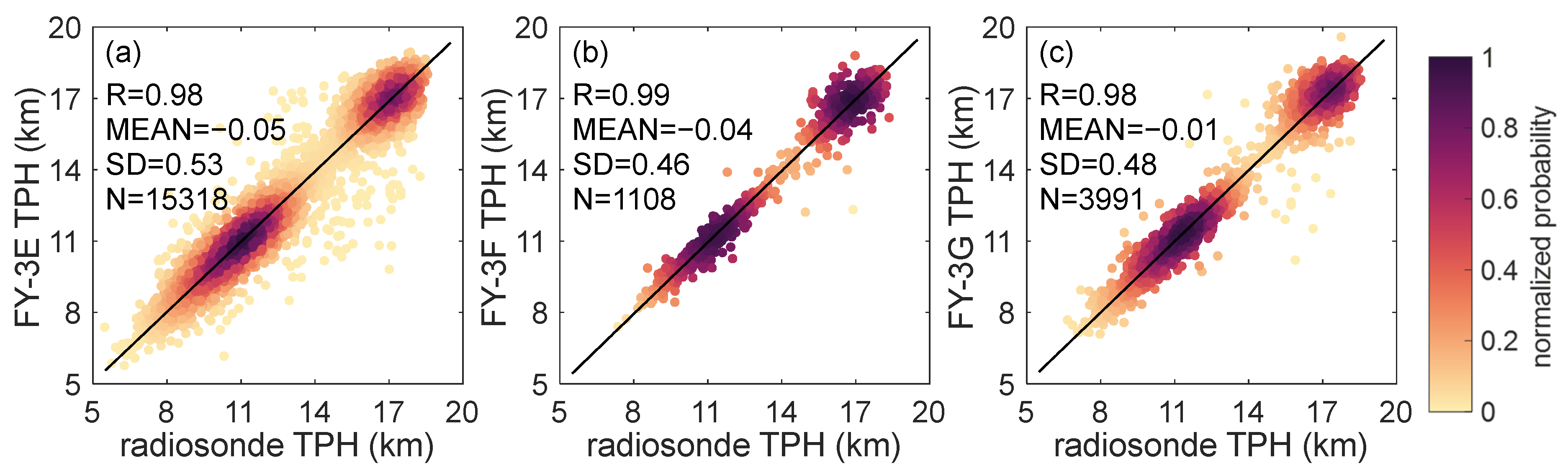
4.2. The TPH Validation

Figure 5 demonstrates a typical example of the temperature profile from FY-3E/BDS RO and collocated radiosonde data. The two observations are highly consistent with each other, and the TPHs obtained were both 8.9 km while the corresponding TPTs were 220.9 K and 220.6 K for RO and radiosonde profiles, respectively. It should be noted that some temperature profiles present more than one very distinct inversion layer. Especially in subtropical jet stream regions, the first tropopause and the second tropopause can coexist, with a difference up to 4–5 km. The WMO criterion used in this study identifies the first tropopause.

Figure 6 shows the correlations between FY-3E, FY-3F, and FY-3G RO and collocated radiosonde TPH. Strong correlations (FY-3E, R = 0.98; FY-3F, R = 0.99; FY-3G, R = 0.98) validated the high accuracy of TPH calculated from FY-3/GNOS-II RO profiles. The mean correlation coefficient obtained by Liu et al. (2019) comparing the TPH of FY-3C with the radiosonde data was 0.93 [38]. In comparison, the results from the FY-3/GNOS-II RO were relatively better. The mean biases between RO and radiosonde TPH are quite small, with −0.05 km for FY-3E, −0.04 km for FY-3F, and −0.01 km for FY-3G. The relatively large SD of 0.53 km for the FY-3E TPH is associated with the fact that radiosonde data are point measurements while RO observations are horizontal averages. Due to the non-uniform distribution of stations across latitudes, the TPH samples were concentrated around 8–14 km and 17–18 km. Therefore, it is highly advantageous to calculate the global TPH by taking the characteristics of the global uniform distribution and the rich data sources that RO data possess.

5. Statistical Analyses of the ABL and Thermal Tropopause from FY-3/GNOS-II RO Profiles

5.1. ABLH Results

The ABLH derived from FY-3/GNOS-II RO refractivity profiles from September 2022 to August 2024 was presented in this section. We first focused on the global ABL detection rate, which was taken for quantifying FY-3/GNOS-II capability on detecting ABL in different regions. Then, the seasonal cycles of ABLH were analyzed.

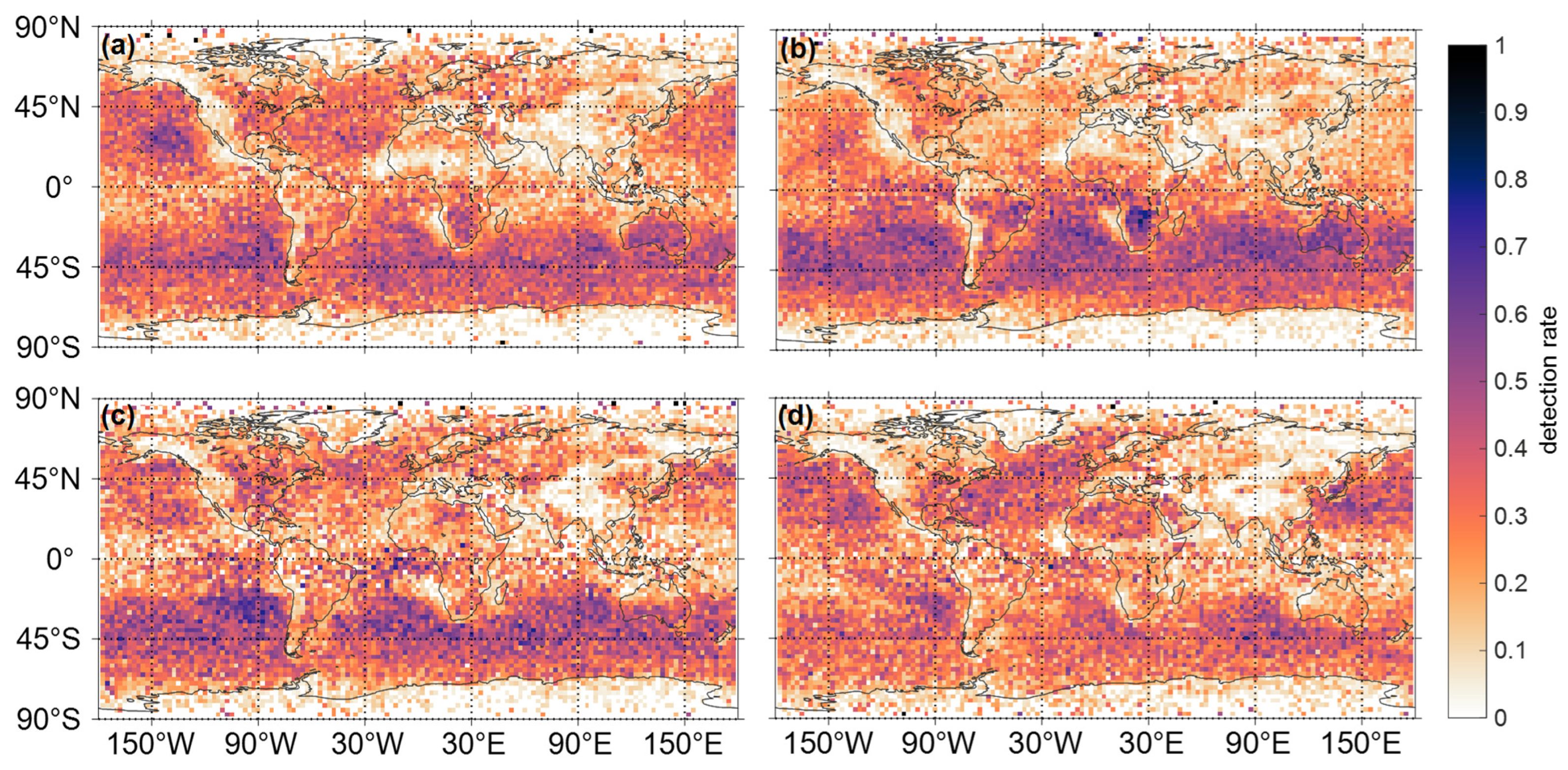
5.1.1. The Detection Rate

Figure 7 shows the global ABL detection rate in NH spring (March–May, MAM), NH summer (June–August, JJA), NH fall (September–November, SON), and NH winter (December–February, DJF). The ABL could frequently be detected over oceans because of their more homogeneous surface and greater thermal inertia, making the ABL generally more stable. It was found that the low detection rate over the equator was caused by strong deep convection in the cloud-covered Intertropical Convergence Zone (ITCZ) lifting the air above the ABL altitude [28]. The detection rate of the FY-3/GNOS-II ABL top was highest over the subtropical eastern Pacific, SH Atlantic, and eastern Indian Ocean, up to 76%. The large-scale subsidence in subtropics suppressed the development of deep convection, making the ABL more stable, and the reduced water vapor and aerosol particles also decreased the attenuation of radio signals. While at high latitudes, small refractivity gradients and shallow ABL made it challenging for FY-3/GNOS-II RO to extract the ABLH. Furthermore, high detection rates were also found over low terrains, such as Australia. In contrast, the detection rate in high-altitude regions (e.g., the Himalayas) was very low throughout the year.

Seasonal variations in the ABL detection rate were only observed in tropical oceans in the prior study that fused RO data from Constellation Observing System for Meteorology, Ionosphere, and Climate (COSMIC), TerraSAR-X, Gravity Recovery and Climate Experiment (GRACE), and Communication and Navigation Outage Forecasting System (CNOFS) [30]. The FY-3/GNOS-II RO results in Figure 7 show more seasonal variations in the ABL detection rate. It was clear that the detection rate in low- and mid-latitude oceans was highest in winter and lowest in summer. This seasonal pattern also occurred over some low-latitude lands. During boreal summer, the Asian monsoon generated extensive deep convection, which reduced the detection rate [11]. The Amazon region often experienced the rainy season, and the detection rate was relatively high only during the JJA season [11]. The ABL inversion in subtropical deserts (e.g., the Sahara, Kalahari, and Greater Australian) was fairly weak in spring and summer [3], resulting in lower detection rates. In tropical regions, detection rates also varied with the seasonality of the ITCZ, as it was located over the north during the NH summer and over the south during the NH winter [46].

5.1.2. Seasonal Cycle

To demonstrate seasonal variations in the ABLH from FY-3/GNOS-II, Figure 8 shows the global ABLH in different seasons, and Figure 9 illustrates the ABLH difference over land and oceans for the JJA season, subtracting the DJF season. As shown, the average ABLH of the North American continent, northern Africa, and Eurasia was about 0.5 km higher in summer than in winter. Similar but weaker seasonality also occurred in Australia, where the ABL was higher during the summer. This seasonality was absent from southern South America and southern Africa, probably due to the smaller land area, which was more influenced by the adjacent ocean ABL. Seasonality over tropical lands could be attributed to the precipitation of the ITCZ, with deeper ABL in dry seasons and shallower ABL in wet seasons [50]. For example, there was a consistent seasonality over a thin range north and south of the equator in Africa, with ABL higher in winter and lower in summer. This seasonal pattern was also observed near the equator in South America, but the variation was relatively weaker. The study by Kalmus et al. (2022) showed similar but stronger seasonal variations, which may be due to differences in the ABLH algorithm or vertical resolution [51]. The seasonal characteristics of the ABLH in Greenland and Antarctica could not be well represented because of the lack of observations (smaller grid area at 2.5° × 2.5° in the polar regions).

Ocean areas with high ABL were distributed within 30°N–30°S in the presence of subtropical high pressure and trade wind belts. Such warm pool areas as the western Pacific, Atlantic, and Indian Oceans featured large ABLH. The change in cloud type and the rise of cold seawater along the west coasts caused regions of the Pacific and Atlantic with higher ABL to deviate westward from the American and African continents [28]. Seasonal variations in the ABLH over oceans were generally less pronounced than the ABLH over land. The ABL over the central regions of the northern Atlantic and northwestern Pacific was slightly higher in winter. This was probably related to the baroclinic systems, which were important factors in the development of frontal systems, cyclones, and other weather systems. In contrast, the ABL in these areas was shallower in summer, related to the fog formation [3]. In addition, the Pacific, Atlantic, and Indian Oceans in 10°S–30°S had higher ABL in winter. This could be explained by the seasonal drift of the pressure belts, causing these regions under the subtropical high pressure in winter and the southeasterly trade wind in summer; hence, the ABL was high in winter and low in summer [48,50]. Overall, these seasonal variations in the ABLH over the NH and SH oceans were consistent with the COSMIC RO and ERA5 results obtained by Ho et al. (2024) using the minimum gradient method to bending angle profiles [33].

5.2. TPH and TPT Results

Here, the TPH and TPT were calculated using FY-3/GNOS-II RO profiles, and the structures and characteristics of the tropopause were investigated.

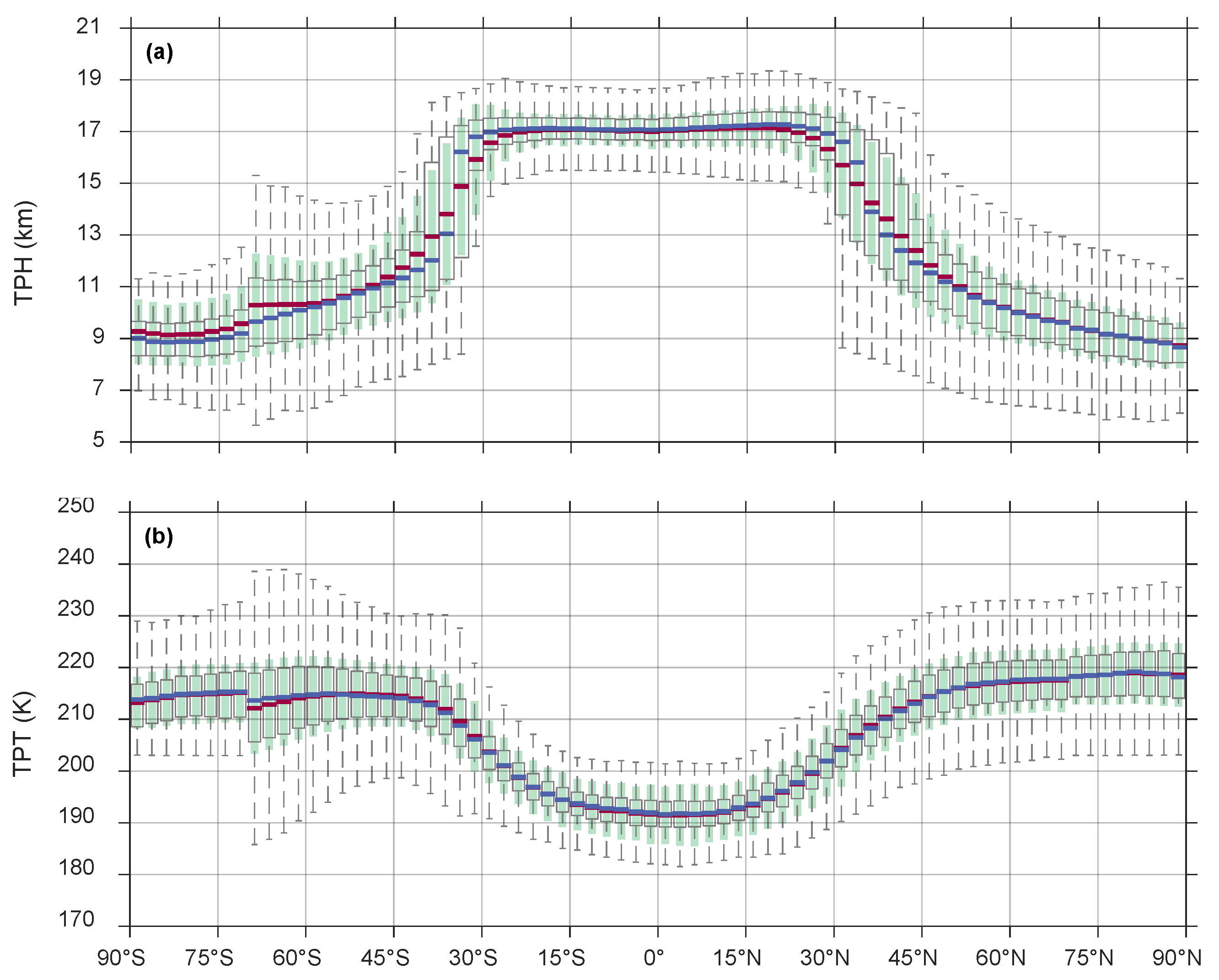
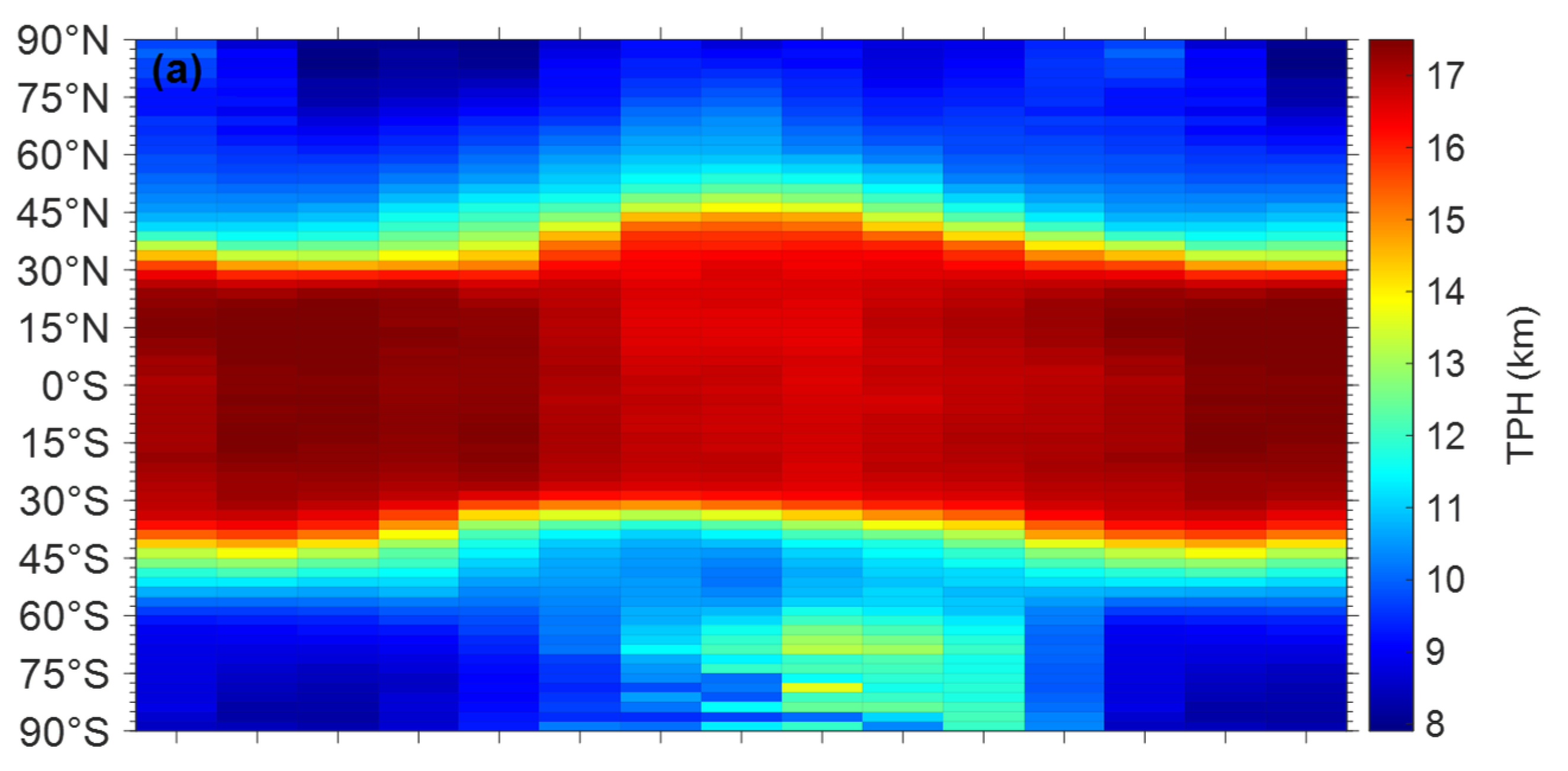
5.2.1. Spatial Structures

Figure 10 and Figure 11, respectively, show the monthly mean TPH and TPT in the MAM, JJA, SON, and DJF seasons. It was evident that the longitudinal variations in both TPH and TPT are less significant than the latitudinal variations. Longitudinal variations were mainly caused by the geographical distribution of land and oceans, and more variations occurred in land regions. Fairly small TPH (7–9 km) and larger TPT (215–220 K) values were observed in northeastern Canada and easternmost Russia, and they were most pronounced in winter. The finding derived from FY-3/GNOS-II was highly consistent with the result of Rieckh et al. (2014) using RO data from CHAMP (Challenging Minisatellite Payload), SAC-C (Satélite de Aplicaciones Científicas-C), COSMIC, and GRACE-A [52]. This zonal asymmetric pattern was caused by the Rossby wave, and the fact that its activity was weakest during the NH summer is shown in Figure 10b and Figure 11b [53]. Zonal asymmetry was also found in the tropics and subtropics. In NH summer, the high tropopause in South Asia could exceed 18 km, also with low temperature, a feature associated with the Asian monsoon [54]. In DJF, the extremely cold tropopause near the west Pacific heating region was directly linked to the large-scale convective heating [54]. In addition, the central South Pacific also exhibited relatively lower and warmer tropopause during the DJF. In contrast to the NH, the TPH and TPT in the SH middle and high latitudes presented highly zonal symmetry.

In terms of latitudinal variations, the TPH generally decreased from the tropics to polar regions, while the TPT followed the opposite trend. Figure 12 shows the TPH and TPT values for each 2.5° latitude interval, including the mean, median, SD, quartiles (25% to 75%), and extreme values. As shown in Figure 12a, the mean TPH was about 17 km within 30°S–30°N. It dropped to 10 km at 60° in both hemispheres and further decreased poleward to 8 km in the remaining high latitudes. The mean and median values were well consistent in the tropics and NH high latitudes. In these two regions, the quartiles covered less than 1 km and 2 km, and the SDs covered 1.5–2 km and 2–3.5 km, respectively. In the NH and SH 20–45°, known as the subtropical jet stream region, the TPH decreased poleward with strong gradients. And there were significant differences between the mean and median values, also with the differences in extreme values reaching up to 10 km. The simultaneous occurrence of the first and second tropopause in these latitudes resulted in the tropopause break that caused large variations in the distribution of TPH. Toward the poles, the median shifted from higher to lower relative to the mean, very much in line with the distribution characteristic of the second tropopause (most frequently occurring in the subtropical jet stream region). In addition, differences were also found between the mean and the median in the 60°S–90°S. The LRT method was not well suited to the extremely cold Antarctic air [53]. The smaller median relative to the mean indicated that a major part of the tropopause was located at lower altitudes.

Latitudinal variations in the TPT in Figure 12b were negatively correlated with the TPH overall. In 15°S–15°N, the highest altitude corresponded to the lowest temperature with mean values of 191–194 K. At 15–45° on both hemispheres, the mean TPT increased poleward from 194 K to 215 K. TPT varied more uniformly across the rest of the middle and high latitudes, showing mean values ranging from 212 K to 219 K. Except for the 60°S–70°S, the mean and median TPTs were essentially equal, with quartiles covering 4–8 K from low to high latitudes, and SDs covering 11–16 K, respectively. In the SH 60–70°, the larger median of TPT compared to the mean was negatively similar to TPH. The minimum TPT decreased to 185 K, and the maximum TPT exceeded 238 K.

5.2.2. Annual Cycle

Figure 13a shows the annual cycle of TPH derived from FY-3/GNOS-II RO measurements. In the NH 0–25°, the tropopause showed a weak annual cycle in which TPH was lowest from July to September and highest during most months of spring and winter. Stratospheric processes could explain this seasonal cycle. One interpretation was the strong tropical upwelling of the Brewer–Dobinson circulation (BDC) NH branch during winter, resulting in the elevation of the tropopause [52]. The TPH was also higher in some spring months, which could be attributed to the combination of extratropical wave forcing from both hemispheres [55]. In the NH middle latitudes of 25–65°, the annual cycle was most pronounced, with the amplitude exceeding 3 km. The tropopause rose from March to August and gradually descended from September onwards. Consistent with previous research, a double wave pattern of the annual cycle was found at latitudes greater than 65°. The tropopause was lowest in NH spring and also relatively low in NH fall, and the increase in latitude made the TPH lower in more spring months. This springtime minimal TPH at high Arctic latitudes was commonly associated with the enhanced downwelling branch of the BDC.

TPH in the SH tropics tended to increase and then decrease from spring to winter, and featured the smallest amplitude variation of less than 1 km. From the SH tropics up to 55°S, TPH was highest in summer and lowest in winter. Most notably, the annual cycle of TPH was obvious at high latitudes beyond 55°S. The lack of incoming radiation at high latitudes in the SH winter led to colder stratospheric temperatures and higher TPH. Slightly different from the results of Rieckh et al. (2014) and Li et al. (2017) [52,56], the higher tropopause continued from July to November, possibly due to differences in observation time periods.

Figure 13b shows the annual cycle of TPT, which was reversed from the TPH in 45°S–45°N and high latitudes southward of 55°S. However, at latitudes northward of 45°N, a single wave pattern of TPT was found, exhibiting the warmest tropopause in summer and the coldest tropopause in winter. In addition, the annual amplitude here was large, with the TPT difference between January and August capable of reaching 18 K. In the SH, the reversal of the annual cycle of TPT occurred at 45°, more northward oriented than the TPH. Note that the winter tropopause over the Antarctic was much colder than in the NH, partly due to the Antarctic polar vortex and also because the NH was more prone to sudden stratospheric warming events. Meanwhile, remarkable amplitude variations in SH high latitudes could exceed 20 K.

6. Discussion

Compared to the previous batch of FY-3 satellites equipped with GNOS [31], the capability of GNOS-II to determine the ABL has been significantly improved because of the enrichment of observations by BDS RO with OL signal tracking mode. For the FY-3/GNOS-II RO results, the ABL detection rate demonstrated more seasonal variations compared to other RO observations [30]. The seasonal pattern of the FY-3/GNOS-II RO ABLH was consistent with previous studies, but the variation was weaker in some regions, such as over land in the tropics. The longitudinal and latitudinal variations in the TPH and TPT were analyzed in detail, and the annual cycles of the TPH and TPT were demonstrated at a higher latitudinal resolution of 2.5° compared to previous studies.

In addition to the research progress in this study, there are still some challenges in using RO data to detect the ABLH, TPH, and TPT. RO data utilization is limited when observing the ABLH because most RO profiles may not penetrate near the surface. RO ABLH and TPH over remote areas and oceans are difficult to validate due to a lack of validation data. In the future, more FY-3 series satellites will be launched. Multiple FY-3 satellite RO observations, as a data source, can be expected to realize more value in local or global, short-term or long-term climate research when combined with other measurements.

7. Conclusions

This work preliminarily validates the capability of ABL and tropopause retrieval from FY-3/GNOS-II BDS and GPS RO observations, notably incorporating the OL tracking results from the BDS occultations. The WCT algorithm is used to identify the ABLH from vertical structures of RO refractivity profiles. The profiles, which penetrate down to the surface altitude of 0.5 km, are employed in FY-3E, FY-3F, and FY-3G ROEs, and their percentages are 48%, 51%, and 51%, respectively. The ABLHs from FY-3E, FY-3F, and FY-3G are highly consistent with the collocated radiosonde observations with correlation coefficients of 0.73, 0.73, and 0.75, respectively. Second, TPH and TPT are obtained from dry pressure and temperature profiles by the LRT method. The correlation coefficients of TPHs derived from FY-3E, FY-3F, and FY-3G with radiosonde-derived TPHs are 0.98, 0.99, and 0.98, respectively. The FY-3/GNOS-II RO retrieved ABL, and tropopause information can be a reliable supplementary data source for weather and climate research or applications. The conclusions of this study are summarized below.

• FY-3/GNOS-II RO profiles show a high detection rate of the ABL top in low and middle latitudes. The highest detection rates are found in the subtropical eastern Pacific, SH Atlantic, and eastern Indian Ocean, up to 76%. The detection rates over low and mid-latitude oceans are higher in winter than in summer, and the same pattern is observed over some low-latitude land regions. Due to weak ABL inversion, the detection rates in subtropical deserts are lower in spring and summer.
• Seasonality of the ABLH derived from FY-3/GNOS-II RO is clear and distinct. It could be observed that ABLH is lower in summer in a narrow range on both sides of the equator in Africa, influenced by the precipitation of the ITCZ. Other common seasonal characteristics of the ABL are also identified.
• The TPH and TPT retrieved from FY-3/GNOS-II RO feature apparent longitudinal and latitudinal characteristics. For example, TPH shows significant zonal asymmetry in northeastern Canada and easternmost Russia due to the Rossby wave. The presence of a double tropopause separates the mean and median values of TPH and TPT at middle latitudes.
• In latitudes northward of 65°N, the annual cycle of TPH exhibits a double wave pattern. While in latitudes greater than 45°N for TPT, a single wave pattern is presented. Furthermore, the annual cycle of the TPH is reversed near 25°N and 55°S. The reversal of the annual cycle for TPT occurs at 25°N, 45°N, and 45°S. These characteristics of the tropopause are clearly captured by FY-3/GNOS-II RO.

References

1. Stull, R.B. An Introduction to Boundary Layer Meteorology; Kluwer Academic: Dordrecht, The Netherlands, 1988; pp. 9–16. [Google Scholar] [CrossRef]
2. Medeiros, B.; Hall, A.; Stevens, B. What Controls the Mean Depth of the PBL? J. Clim. 2005, 18, 3157–3172. [Google Scholar] [CrossRef]
3. von Engeln, A.; Teixeira, J. A Planetary Boundary Layer Height Climatology Derived from ECMWF Reanalysis Data. J. Clim. 2013, 26, 6575–6590. [Google Scholar] [CrossRef]
4. Garratt, J.R. Sensitivity of Climate Simulations to Land-Surface and Atmospheric Boundary-Layer Treatments—A Review. J. Clim. 1993, 6, 419–448. [Google Scholar] [CrossRef]
5. Ho, S.P.; Anthes, R.A.; Ao, C.O.; Healy, S.; Horanyi, A.; Hunt, D.; Mannucci, A.J.; Pedatella, N.; Randel, W.J.; Simmons, A.; et al. The COSMIC/FORMOSAT-3 Radio Occultation Mission after 12 Years: Accomplishments, Remaining Challenges, and Potential Impacts of COSMIC-2. Bull. Amer. Meteor. Soc. 2020, 101, E1107–E1136. [Google Scholar] [CrossRef]
6. Holton, J.R.; Haynes, P.H.; McIntyre, M.E.; Douglass, A.R.; Rood, R.B.; Pfister, L. Stratosphere-troposphere exchange. Rev. Geophys. 1995, 33, 403–439. [Google Scholar] [CrossRef]
7. Schmidt, T.; Heise, S.; Wickert, J.; Beyerle, G.; Reigber, C. GPS radio occultation with CHAMP and SAC-C: Global monitoring of thermal tropopause parameters. Atmos. Chem. Phys. 2005, 5, 1473–1488. [Google Scholar] [CrossRef]
8. Seidel, D.J.; Ao, C.O.; Li, K. Estimating climatological planetary boundary layer heights from radiosonde observations: Comparison of methods and uncertainty analysis. J. Geophys. Res. 2010, 115, D16113. [Google Scholar] [CrossRef]
9. Pietroni, I.; Argentini, S.; Petenko, I.; Sozzi, R. Measurements and Parametrizations of the Atmospheric Boundary-Layer Height at Dome C. Bound.-Layer Meteor. 2012, 143, 189–206. [Google Scholar] [CrossRef]
10. Li, H.; Yang, Y.; Hu, X.M.; Huang, Z.; Wang, G.; Zhang, B.; Zhang, T. Evaluation of retrieval methods of daytime convective boundary layer height based on lidar data. J. Geophys. Res. Atmos. 2017, 122, 4578–4593. [Google Scholar] [CrossRef]
11. McGrath-Spangler, E.L.; Denning, A.S. Global seasonal variations of midday planetary boundary layer depth from CALIPSO space-borne LIDAR. J. Geophys. Res. Atmos. 2013, 118, 1226–1233. [Google Scholar] [CrossRef]
12. Fetzer, E.J.; Teixeira, J.; Olsen, E.T.; Fishbein, E.F. Satellite remote sounding of atmospheric boundary layer temperature inversions over the subtropical eastern Pacific. Geophys. Res. Lett. 2004, 31, L17102. [Google Scholar] [CrossRef]
13. Wood, R.; Bretherton, C.S. Boundary Layer Depth, Entrainment, and Decoupling in the Cloud-Capped Subtropical and Tropical Marine Boundary Layer. J. Clim. 2004, 17, 3576–3588. [Google Scholar] [CrossRef]
14. Santer, B.D.; Wehner, M.F.; Wigley, T.M.L.; Sausen, R.; Meehl, G.A.; Taylor, K.E.; Ammann, C.; Arblaster, J.; Washington, W.M.; Boyle, J.S.; et al. Contributions of Anthropogenic and Natural Forcing to Recent Tropopause Height Changes. Science 2003, 301, 479–483. [Google Scholar] [CrossRef] [PubMed]
15. Feng, S.; Fu, Y.; Xiao, Q. Trends in the global tropopause thickness revealed by radiosondes. Geophys. Res. Lett. 2012, 39, L20706. [Google Scholar] [CrossRef]
16. Thuburn, J.; Craig, G.C. GCM Tests of Theories for the Height of the Tropopause. J. Atmos. Sci. 1997, 54, 869–882. [Google Scholar] [CrossRef]
17. Thuburn, J.; Craig, G.C. Stratospheric Influence on Tropopause Height: The Radiative Constraint. J. Atmos. Sci. 2000, 57, 17–28. [Google Scholar] [CrossRef]
18. Vernier, J.P.; Thomason, L.W.; Kar, J. CALIPSO detection of an Asian tropopause aerosol layer. Geophys. Res. Lett. 2011, 38, L07804. [Google Scholar] [CrossRef]
19. Kursinski, E.R.; Hajj, G.A.; Bertiger, W.I.; Leroy, S.S.; Meehan, T.K.; Romans, L.J.; Schofield, J.T.; McCleese, D.J.; Melbourne, W.G.; Thornton, C.L.; et al. Initial results of radio occultation of Earth’s atmosphere using the global positioning system. Science 1996, 271, 1107–1110. [Google Scholar] [CrossRef]
20. Kursinski, E.R.; Hajj, G.A.; Schofield, J.T.; Linfield, R.P.; Hardy, K.R. Observing Earth’s atmosphere with radio occultation measurements using the Global Positioning System. J. Geophys. Res. 1997, 102, 23429–23465. [Google Scholar] [CrossRef]
21. Ao, C.O.; Waliser, D.E.; Chan, S.K.; Li, J.L.; Tian, B.; Xie, F.; Mannucci, A.J. Planetary boundary layer heights from GPS radio occultation refractivity and humidity profiles. J. Geophys. Res. 2012, 117, D16117. [Google Scholar] [CrossRef]
22. Ratnam, M.V.; Tetzlaff, G.; Jacobi, C. Structure and Variability of the Tropopause Obtained from CHAMP Radio Occultation Temperature Profiles. In Earth Observation with CHAMP; Reigber, C., Lühr, H., Schwintzer, P., Wickert, J., Eds.; Springer: Berlin/Heidelberg, Germany, 2005; pp. 579–584. [Google Scholar] [CrossRef]
23. von Engeln, A.; Teixeira, J.; Wickert, J.; Buehler, S.A. Using CHAMP radio occultation data to determine the top altitude of the Planetary Boundary Layer. Geophys. Res. Lett. 2005, 32, L06815. [Google Scholar] [CrossRef]
24. Sokolovskiy, S.V.; Rocken, C.; Hunt, D.; Schreiner, W.; Johnson, J.; Masters, D.; Esterhuizen, S. GPS profiling of the lower troposphere from space: Inversion and demodulation of the open-loop radio occultation signals. Geophys. Res. Lett. 2006, 33, L14816. [Google Scholar] [CrossRef]
25. Guo, S.; Zhang, S.; He, Y.; Wang, S.; Sheng, Z.; Meng, X.; Yu, T. Optimizing GPS L2P radio occultation processing for COSMIC-2 atmospheric bending angle retrieval. IEEE Trans. Geosci. Remote Sens. 2025, 63, 4102410. [Google Scholar] [CrossRef]
26. Sokolovskiy, S.V.; Kuo, Y.H.; Rocken, C.; Schreiner, W.; Hunt, D.; Anthes, R.A. Monitoring the atmospheric boundary layer by GPS radio occultation signals recorded in the open-loop mode. Geophys. Res. Lett. 2006, 33, L12813. [Google Scholar] [CrossRef]
27. Sokolovskiy, S.V.; Rocken, C.; Lenschow, D.H.; Kuo, Y.H.; Anthes, R.A.; Schreiner, W.; Hunt, D. Observing the moist troposphere with radio occultation signals from COSMIC. Geophys. Res. Lett. 2007, 34, L18802. [Google Scholar] [CrossRef]
28. Guo, P.; Kuo, Y.H.; Sokolovskiy, S.V.; Lenschow, D.H. Estimating Atmospheric Boundary Layer Depth Using COSMIC Radio Occultation Data. J. Atmos. Sci. 2011, 68, 1703–1713. [Google Scholar] [CrossRef]
29. Ho, S.P.; Liang, P.; Anthes, R.A.; Kuo, Y.H.; Lin, H.C. Marine Boundary Layer Heights and Their Longitudinal, Diurnal, and Interseasonal Variability in the Southeastern Pacific Using COSMIC, CALIOP, and Radiosonde Data. J. Clim. 2015, 28, 2856–2872. [Google Scholar] [CrossRef]
30. Basha, G.; Kishore, P.; Ratnam, M.V.; Babu, S.R.; Velicogna, I.; Jiang, J.H.; Ao, C.O. Global climatology of planetary boundary layer top obtained from multi-satellite GPS RO observations. Clim. Dyn. 2019, 52, 2385–2398. [Google Scholar] [CrossRef]
31. Zhu, Z.; Xu, X.; Luo, J. Inversion and Analysis of Atmospheric Boundary Layer Height Using FY-3C Radio Occultation Refractive Index Data. Geomat. Inf. Sci. Wuhan Univ. 2021, 46, 395–401. [Google Scholar] [CrossRef]
32. Santosh, M. Estimation of daytime planetary boundary layer height (PBLH) over the tropics and subtropics using COSMIC-2/FORMOSAT-7 GNSS–RO measurements. Atmos. Res. 2022, 279, 106361. [Google Scholar] [CrossRef]
33. Ho, S.P.; Gu, G.; Zhou, X. The Planetary Boundary Layer Height Climatology Over Oceans Using COSMIC-2 and Spire GNSS RO Bending Angles From 2019 to 2023: Comparisons to CALIOP, ERA-5, MERRA2, and CFS Reanalysis. IEEE Trans. Geosci. Remote Sens. 2024, 62, 5803314. [Google Scholar] [CrossRef]
34. He, Y.; Zhang, S.; Guo, S.; Wu, Y. Quality Assessment of the Atmospheric Radio Occultation Profiles from FY-3E/GNOS-II BDS and GPS Measurements. Remote Sens. 2023, 15, 5313. [Google Scholar] [CrossRef]
35. Randel, W.J.; Wu, F.; Rivera Ríos, W. Thermal variability of the tropical tropopause region derived from GPS/MET observations. J. Geophys. Res. 2003, 108, 4024. [Google Scholar] [CrossRef]
36. Schmidt, T.; Wickert, J.; Beyerle, G.; Reigber, C. Tropical tropopause parameters derived from GPS radio occultation measurements with CHAMP. J. Geophys. Res. 2004, 109, D13105. [Google Scholar] [CrossRef]
37. Son, S.W.; Tandon, N.F.; Polvani, L.M. The fine-scale structure of the global tropopause derived from COSMIC GPS radio occultation measurements. J. Geophys. Res. 2011, 116, D20113. [Google Scholar] [CrossRef]
38. Liu, Z.; Sun, Y.; Bai, W.; Xia, J.; Tan, G.; Cheng, C.; Du, Q.; Wang, X.; Zhao, D.; Tian, Y.; et al. Validation of Preliminary Results of Thermal Tropopause Derived from FY-3C GNOS Data. Remote Sens. 2019, 11, 1139. [Google Scholar] [CrossRef]
39. Liu, Z.; Sun, Y.; Bai, W.; Xia, J.; Tan, G.; Cheng, C.; Du, Q.; Wang, X.; Zhao, D.; Tian, Y.; et al. Comparison of RO tropopause height based on different tropopause determination methods. Adv. Space Res. 2021, 67, 845–857. [Google Scholar] [CrossRef]
40. Li, W.; Sun, Y.; Bai, W.; Yin, C.; Du, Q.; Liu, C.; Wang, X.; Hu, X.; Yang, G.; Xiao, X. Machine Learning methods of FY-3C tropopause product correction. In Proceedings of the 2021 IEEE Specialist Meeting on Reflectometry Using GNSS and Other Signals of Opportunity (GNSS+R), Beijing, China, 14–17 September 2021; pp. 50–52. [Google Scholar] [CrossRef]
41. Sun, Y.; Liu, C.; Du, Q.; Wang, X.; Bai, W.; Kirchengast, G.; Xia, J.; Meng, X.; Wang, D.; Cai, Y.; et al. Global Navigation Satellite System Occultation Sounder II (GNOS II). In Proceedings of the 2017 IEEE International Geoscience and Remote Sensing Symposium (IGARSS). Fort Worth, TX, USA, 23–28 July 2017. pp. 1189–1192. [CrossRef]
42. Liao, M.; Zhang, P.; Yang, G.; Bi, Y.; Liu, Y.; Bai, W.; Meng, X.; Du, Q.; Sun, Y. Preliminary validation of the refractivity from the new radio occultation sounder GNOS/FY-3C. Atmos. Meas. Tech. 2016, 9, 781–792. [Google Scholar] [CrossRef]
43. Liu, C.; Liao, M.; Sun, Y.; Wang, X.; Liang, J.; Hu, X.; Zhang, P.; Yang, G.; Liu, Y.; Wang, J.; et al. Preliminary Assessment of BDS Radio Occultation Retrieval Quality and Coverage Using FY-3E GNOS II Measurements. Remote Sens. 2023, 15, 5011. [Google Scholar] [CrossRef]
44. He, B.; Bao, Q.; Wang, X.; Zhou, L.; Wu, X.; Liu, Y.; Wu, G.; Chen, K.; He, S.; Hu, W.; et al. CAS FGOALS-f3-L model datasets for CMIP6 historical Atmospheric Model Intercomparison Project simulation. Adv. Atmos. Sci. 2019, 36, 771–778. [Google Scholar] [CrossRef]
45. Hersbach, H.; Bell, B.; Berrisford, P.; Biavati, G.; Horányi, A.; Muñoz Sabater, J.; Nicolas, J.; Peubey, C.; Radu, R.; Rozum, I.; et al. ERA5 Monthly Averaged Data on Single Levels from 1940 to Present. Land-Sea Mask Data. 2023. Available online: https://cds.climate.copernicus.eu/datasets/reanalysis-era5-single-levels-monthly-means?tab=overview (accessed on 5 August 2024).
46. Ratnam, M.V.; Basha, S.G. A robust method to determine global distribution of atmospheric boundary layer top from COSMIC GPS RO measurements. Atmosph. Sci. Lett. 2010, 11, 216–222. [Google Scholar] [CrossRef]
47. Brooks, I.M. Finding Boundary Layer Top: Application of a Wavelet Covariance Transform to Lidar Backscatter Profiles. J. Atmos. Ocean. Technol. 2023, 20, 1092–1105. [Google Scholar] [CrossRef]
48. Xu, X.; Liu, S.; Luo, J. Analysis on the Variation of Global ABL Top Structure Using COSMIC Radio Occultation Refractivity. Geomat. Inf. Sci. Wuhan Univ. 2018, 43, 94–100. [Google Scholar] [CrossRef]
49. Reichler, T.; Dameris, M.; Sausen, R. Determining the tropopause height from gridded data. Geophys. Res. Lett. 2003, 30, 2042. [Google Scholar] [CrossRef]
50. Chan, K.M.; Wood, R. The seasonal cycle of planetary boundary layer depth determined using COSMIC radio occultation data. J. Geophys. Res. Atmos. 2013, 118, 12422–12434. [Google Scholar] [CrossRef]
51. Kalmus, P.M.; Ao, C.O.; Wang, K.N.; Manzi, M.P.; Teixeira, J. A high-resolution planetary boundary layer height seasonal climatology from GNSS radio occultations. Remote Sens. Environ. 2022, 276, 113037. [Google Scholar] [CrossRef]
52. Rieckh, T.; Scherllin-Pirscher, B.; Ladstädter, F.; Foelsche, U. Characteristics of tropopause parameters as observed with GPS radio occultation. Atmos. Meas. Tech. 2014, 7, 3947–3958. [Google Scholar] [CrossRef]
53. Zängl, G.; Hoinka, K.P. The Tropopause in the Polar Regions. J. Clim. 2001, 14, 3117–3139. [Google Scholar] [CrossRef]
54. Highwood, E.J.; Hoskins, B.J. The tropical tropopause. Q. J. R. Meteorol. Soc. 1998, 124, 1579–1604. [Google Scholar] [CrossRef]
55. Reid, G.C.; Gage, K.S. The tropical tropopause over the western Pacific: Wave driving, convection, and the annual cycle. J. Geophys. Res. 1996, 101, 21233–21241. [Google Scholar] [CrossRef]
56. Li, W.; Yuan, Y.; Chai, Y.; Liou, Y.; Ou, J.; Zhong, S. Characteristics of the global thermal tropopause derived from multiple radio occultation measurements. Atmos. Res. 2017, 185, 142–157. [Google Scholar] [CrossRef]
Figure 1. Stacked ROEs numbers for FY-3/GNOS-II from 1 September 2022 (DOY 244) to 31 August 2024 (DOY 244).
Remotesensing 17 02126 g001
Figure 2. The spatial coverage of FY-3/GNOS-II ROEs.
Remotesensing 17 02126 g002
Figure 3. An example of FY-3E/BDS ROE on 19 April 2023 (at −79.86°W, 25.77°N, 1115 UTC) and collocated radiosonde refractivity profile detecting the ABL top by WCT method: (a) The matched RO and radiosonde refractivity. (b) Their covariance transforms and ABLH.
Remotesensing 17 02126 g003
Figure 4. Scatter plots showing the correlations of the ABLH derived from collocated FY-3/GNOS-II RO and radiosonde refractivity. The density of points is linearly mapped to the color bar: (a) ABLH correlation between the FY-3E RO and radiosonde data, containing the correlation coefficients (R), mean bias (MEAN), standard deviation (SD), and number of samples (N). (b) Same as (a), but for FY-3F and radiosonde data. (c) Same as (a), but for FY-3G and radiosonde data.
Remotesensing 17 02126 g004
Figure 5. An example of FY-3E/BDS ROE on March 1, 2023 (at −58.95°W, 48.32°N, 1011 UTC) and collocated radiosonde temperature profiles detecting the tropopause.
Remotesensing 17 02126 g005
Figure 6. Scatter plots showing the correlations between the TPH calculated from FY-3/GNOS-II RO and radiosonde profiles. The density of points is linearly mapped to the color bar: (a) TPH correlation between the FY-3E RO and radiosonde data, containing the R, MEAN, SD, and N. (b) Same as (a), but for FY-3F and radiosonde data. (c) Same as (a), but for FY-3G and radiosonde data.
Remotesensing 17 02126 g006
Figure 7. The ABL detection rate observed from FY-3/GNOS-II RO profiles in different seasons from September 2022 to August 2024 on 2.5° × 2.5° latitude–longitude grids: (a) MAM, (b) JJA, (c) SON, (d) DJF.
Remotesensing 17 02126 g007
Figure 8. Global distribution of the ABLH derived from FY-3/GNOS-II RO measurements during different seasons from September 2022 to August 2024 on 2.5° × 2.5° latitude–longitude grids: (a) MAM, (b) JJA, (c) SON, (d) DJF.
Remotesensing 17 02126 g008
Figure 9. ABLH difference over lands (a) and oceans (b) found by subtracting DJF from JJA gridded to 2.5° × 2.5°, using the FY-3/GNOS-II RO measurements from September 2022 to August 2024.
Remotesensing 17 02126 g009
Figure 10. Global TPH derived from FY-3/GNOS-II RO measurements during different seasons from September 2022 to August 2024 on 2.5° × 2.5° latitude–longitude grids: (a) MAM, (b) JJA, (c) SON, (d) DJF.
Remotesensing 17 02126 g010
Figure 11. Global TPT derived from FY-3/GNOS-II RO measurements during different seasons from September 2022 to August 2024 on 2.5° × 2.5° latitude–longitude grids: (a) MAM, (b) JJA, (c) SON, (d) DJF.
Remotesensing 17 02126 g011
Figure 12. TPH (a) and TPT (b) versus latitude from September 2022 to August 2024. Shown are the mean (red line), median (blue line), SD (green bars), 25 to 75 quartile (black box), and extreme values (whiskers) for 2.5° latitudinal bands.
Remotesensing 17 02126 g012
Figure 13. Annual cycle of monthly mean TPH (a) and TPT (b) from September 2022 to August 2024. For clarity, two extra months are shown on the right side of the full cycle.
Remotesensing 17 02126 g013aRemotesensing 17 02126 g013b