Using Sentinel Imagery for Mapping and Monitoring Small Surface Water Bodies

Abstract

Increasing water demand and climate change exacerbate water management challenges in arid and semi-arid regions experiencing water scarcity resulting from low and irregular precipitation and high evapotranspiration. These regions rely on substantial water storage capacity, typically provided by large multi-purpose public reservoirs and small private reservoirs. While public reservoirs are typically monitored, the number, size, and private ownership of small reservoirs complicate effective storage monitoring, hindering efforts to assess water availability during droughts and to allocate water efficiently and equitably. Remote sensing provides a solution to complement existing monitoring systems by offering high spatial and temporal resolution observations. This study introduces a methodology for monitoring the surface area of large and small reservoirs based on optical and radar images from Sentinel-1 and Sentinel-2 satellites. The Normalized Difference Water Index (NDWI) and the Otsu image segmentation method are employed to identify and estimate water body areas, and the Google Earth Engine and programming languages are used to automate the process. The validation results demonstrated correlation for most reservoirs, with slight underestimations at flood peaks. Among the 17 large reservoirs, 16 had an R² value above 0.82, 12 had an RMSE value below 0.8, and 14 had a KGE value above 0.7. For the small reservoirs, the method correctly identified 3224 of the 6370 reservoirs recorded in situ, with greater accuracy in the classes of reservoirs with elevation above 10 m. A total of 7251 reservoirs were mapped, including 4027 not present in the database of the responsible regulatory entity, most with an area of less than 1.8 ha. Performance was better for larger areas (>3 ha), while small areas were underestimated. This methodology offers a practical water management tool adaptable for various-sized surface water bodies, including small, unmonitored water bodies.

1. Introduction

Inland surface water bodies, such as lakes, rivers, wetlands, and reservoirs, are vital components of the water system, providing essential services such as freshwater supply, habitat for biodiversity, flood regulation, hydroelectric power generation, irrigation support, and recreational opportunities. Notably, they support a substantial part of the water demand for agriculture, domestic and industrial uses, and hydropower production [1]. Climate change and human activities have intensified pressures on these water bodies, negatively impacting their environmental conditions and the health surrounding ecosystems. Climate variability, coupled with rising water demands, further amplifies seasonal and annual fluctuations in their storage and surface extent, potentially leading to the shrinkage or disappearance of lakes, rivers, and wetlands [2,3].

Arid and semi-arid regions are especially vulnerable to the pressures arising from human-induced water demand dynamics and climate change [4,5,6]. These regions face irregular precipitation patterns, high evapotranspiration rates, and recurrent drought periods, all of which are aggravated by climate change. In addition, increasing water demands, mainly for irrigation, increase the risk of water scarcity and threaten the viability of many economic activities and the well-being of the population. When groundwater resources are limited, the storage capacity required to balance water availability and demand is typically provided by large multi-purpose public reservoirs and small private reservoirs. The number and location of some of these small reservoirs is often unknown to water managers when the permitting issuance process was not dully followed. Moreover, while public reservoirs are typically monitored, the number, size, and private ownership of small reservoirs complicates effective storage monitoring, hindering efforts to assess water availability during droughts and to allocate water efficiently and equitably. This paper specifically addresses the issue of monitoring small man-made water bodies in arid and semi-arid regions, whose location and extent are often unknown to water managers and which are seldom routinely monitored.

The monitoring of inland waters is crucial to understand their spatial and temporal distributions, to assess their environmental status, including surface extent and volume, and to evaluate their long-term capacity to support various water uses in alignment with the Sustainable Development Goals (SDGs) [7,8]. In situ monitoring of surface water bodies is a costly and resource-intensive approach, which is particularly challenging in remote areas or when assessing many small water bodies. Remote sensing provides a cost-effective alternative, enhancing existing monitoring systems while reducing reliance on expensive field surveys and enforcement activities. By offering high-resolution spatial and temporal observations with increasing accuracy, remote sensing significantly improves water body assessment and management [9,10].

The use of remote sensing for monitoring and mapping water bodies has advanced significantly, with studies employing diverse methods across varying spatial and temporal resolutions [11,12,13]. Early global surface water monitoring efforts utilized Landsat imagery, available since the 1970s [10,14,15]. With 8 days repeat coverage and 30 m resolution, Landsat enables long-term monitoring but struggles with precise water–land boundary detection, leading to significant omission errors. Launched later, MODIS missions also contributed significantly to long-term surface water monitoring [16,17]. While MODIS provides daily global coverage, its coarse resolution limits its ability of detection to water bodies exceeding 500 m in width [11,13]. Both MODIS and Landsat are passive optical sensors that capture reflected sunlight and emitted thermal radiation from the Earth’s surface. They operate in the visible, near-infrared, shortwave infrared, and thermal infrared regions of the electromagnetic spectrum to provide high-resolution imagery suitable for visual interpretation. They are, however, constrained by weather conditions, in particular cloud cover.

Radar satellite sensors, specifically synthetic-aperture radar (SAR), offer the capacity to operate day and night, providing continuous monitoring regardless of weather conditions. Their high-resolution imaging offers wide coverage, rapid scanning, and the ability to monitor small objects with detail. Radar images are often less intuitive to interpret due to their lack of color information and over sensitivity, including interferences. Increasingly, Earth observation scientists are integrating optical and radar data to enhance analysis, leading to more accurate land cover classification, improved environmental monitoring, and better-informed decision-making across various fields.

Sentinel-1 and Sentinel-2 are two satellite families from the Copernicus program of the European Space Agency (ESA). Together these missions offer high-resolution optical imagery from the visible, near-infrared (NIR), and shortwave infrared (SWIR) parts of the spectrum, as well as synthetic-aperture radar (SAR) technology. When coupled with innovative mapping techniques, Sentinel imagery offers new opportunities for precise reservoir delineation.

Water body mapping methodologies have advanced significantly with improving boundary accuracy and enabling the application of remote sensing techniques beyond large reservoirs to smaller, often unmonitored water bodies. The earlier approaches include spectral indices like NDWI and Modified NDWI (MNDWI) [12,14] and classification algorithms such as Random Forest and Artificial Neural Networks [18]. Image thresholding techniques, including the Otsu method, have also been extensively explored [19,20].

The Otsu method has demonstrated effectiveness among these thresholding techniques, outperforming several water body detection techniques [21,22]. The simplicity and efficiency of Otsu’s thresholding approach reduces processing time while maintaining accuracy when compared to classification techniques [21]. The Otsu method starts by segmenting the image by analyzing pixel intensity distributions, and then determines an optimal threshold that maximizes the variance between the object and the background classes, resulting in binary image segmentation [23]. This method is particularly effective in SAR imagery, where grayscale variations correspond to microwave backscatter differences in water, vegetation, and soil [24].

A critical limitation in reservoir mapping is the lack of validation using ground-truth data. Despite the existence of several studies in this field, many methodologies rely on qualitative comparisons without direct validation against in situ data. Ghansah et al. (2022) [18] applied Random Forest classification to Sentinel-2 imagery to map small reservoirs and results were validated through Google Earth images (GEE); Tan et al. (2023) [20] introduced an Otsu-based self-adaptive threshold for automatic water extraction from Sentinel-1 SAR imagery and the results were validated based on a comparison to Sentinel-2 images and global water datasets.

To address this gap, this study performs a spatial–temporal analysis of 17 large reservoirs across the Sado, Sorraia, and Guadiana river basins in southern Portugal, generating a time series of wet surface estimates for each reservoir. The proposed methodology integrates both optical and radar remote sensing data by combining NDWI with the Otsu method applied to Sentinel-1 SAR images. This approach was coded and implemented within the GEE platform, enabling large-scale and automated geospatial analysis [25]. The results were compared to in situ monitoring data to evaluate the performance of the proposed method. Additionally, the method was applied to identify and estimate the surface of small reservoirs (greater than 400 m²), with the results being compared with data from the National Water Authority. It is important to emphasize that the methodology serves both large and small reservoirs; for large public reservoirs the primary focus is to monitor changes in surface area and stored volume over time, while for smaller private reservoirs the aim is limited to their identification and the surface area estimation at the end of winter.

The objectives of this study are as follows: (1) to develop a methodology for accurately mapping reservoir surface areas using spectral indices and segmentation techniques applied to Sentinel-1 and Sentinel-2 imagery; (2) to obtain the reservoir surface area of the 17 monitored reservoirs in southern Portugal, between 2017 and 2023, using an automated GEE workflow; (3) to apply this methodology to identify small reservoirs in the study area; and (4) to validate results using in situ data from Portugal’s national water management authority.

2. Data and Methods

2.1. Image Selection

The study utilizes data from the synthetic-aperture radar (SAR) and multispectral instrument (MSI) sensors aboard the Sentinel-1 and Sentinel-2 satellites to identify and delineate surface water bodies. For large public reservoirs, the primary objective is to monitor the evolution of their surface area and stored volume over time. For smaller private reservoirs, the focus—at this stage of the research—is more limited, aiming to identify their locations and estimate their surface area at the end of winter. Data acquisition and processing were conducted using the GEE cloud platform. The analysis covered the period from October 2017 to October 2023.

As a first step, Sentinel-2 images were selected from the last seven days of each month, provided they had cloud coverage below 15%. The timeframe criteria (last seven days of each month) were chosen to enable direct comparison with data from the in situ monitoring system of water levels, surface area, and stored volume of large reservoirs. From this initial selection, images corresponding to periods of high, moderate, and low precipitation, according to monthly data available in the National Water Resources Information System (SNIRH), were identified to assess surface area fluctuations across large public reservoirs, defining three distinct scenarios (

Table 1. Selection of dates for Sentinel-2 images according to the different precipitation levels during each hydrological year.

Hydrologic Year	High Precipitation Rate	Moderate Precipitation Rate	Low Precipitation Rate
2017–2018	March	November	July
2018–2019	November	March	July
2019–2020	November	March	July
2020–2021	December	April	August
2021–2022	December	April	August
2022–2023	December	April	August

). To cover the entire study area, each mosaic required 6 scenes, resulting in a total of 18 mosaics per scenario and 108 Sentinel-2 images overall.

The identification and characterization of small private reservoirs relied solely on Sentinel-2 images from the last seven days of March 2023, the final month of the wet season. This period was chosen to capture the largest possible surface area, when reservoirs are at peak water volume, as the primary research objective is to evaluate the method’s effectiveness in identifying small reservoirs without conducting a temporal analysis. To cover the entire study area, a mosaic of six scenes from March 2023 was required, totaling six Sentinel-2 images.

In the second step, Sentinel-1 SAR images from the last seven days of each month were selected for the period from October 2017 to October 2023. Only single VV polarization with vertical transmission/reception in the interferometric wide (IW) mode was used, as it is more effective for water extraction [26]. To cover the entire study area, each mosaic required 3 Sentinel-1 scenes, resulting in a total of 72 mosaics and 216 SAR images over the study period. For the analysis of small reservoirs, only images from the last seven days of March 2023 were used, with a single mosaic of three SAR scenes covering the full study area.

2.2. Extraction of Water Surface Area from Satellite Images

Figure 1 illustrates the methodology used to delineate water bodies from the selected images. This approach combines the Normalized Difference Water Index (NDWI) derived from Sentinel-2 optical images with the Otsu algorithm applied to Sentinel-1 SAR images. The Otsu algorithm is a fast and automatic image segmentation method that determines an optimal threshold by maximizing the variance between foreground and background classes [23]. This adaptive thresholding technique is particularly effective for SAR images, where variations in gray values enhance the distinction of water bodies.

However, the Otsu algorithm performs best with bimodal images and when the target object occupies at least 10% of the total area [27]. To meet this criterion, the NDWI is first applied to identify potential water body regions within the image. The Otsu method is then applied exclusively to these identified areas, rather than the entire image, improving segmentation accuracy.

Inter-annual variations in reservoir surface area make it challenging to accurately delineate water body boundaries over time. Furthermore, NDWI is sensitive to wet surfaces, clouds, and other terrain features that can obscure target water bodies, particularly in the case of small reservoirs. To address these challenges, we defined stable areas of interest by applying buffers corresponding to the three scenarios described in Table 1 around the regions identified by NDWI. Tests were conducted using different buffer sizes applied to SAR images, and for standardization purposes a single buffer distance of 100 m was selected to apply to all reservoirs. This distance was chosen based on the cases that produced the most accurate segmentation according to the Otsu thresholding method, which assumes that the cropped image displays a bimodal pixel frequency histogram [23]. Within these areas, the Otsu technique was implemented to improve water body extraction.

The steps illustrated in Figure 1 are described below:

1. The Normalized Water Index (NDWI) developed by McFeeters (1996) [28] is computed from Sentinel 2 images, using the band 3 (green) and band 8 (near-infrared) of multispectral sensors to delimit the presence of water on the surface in digital images (a), as described in the following Equation (1):

$$\mathrm{N}\mathrm{D}\mathrm{W}\mathrm{I}={\displaystyle \frac{{\rho }_{green}-{\rho }_{nir}}{{\rho }_{green}+{\rho }_{nir}}}$$

(1)

2. A preliminary boundary of the water bodies is obtained from the NDWI dataset (a). Using recommendations from Pena-Regueiro et al. (2020) [29] for Sentinel-2 data, the water body mask was generated, considering only NDWI pixels above −0.2 (b).

3. Buffers of 100 m around the water body mask were defined for high, moderate, and low precipitation scenarios to represent water fluctuations for each reservoir throughout the hydrological year (c).

4. The SAR images are cropped using the buffer polygon (d). Since the reservoir surface area varies significantly after rainfall, each buffer served as a reference for selecting and cropping images from the corresponding month and the three subsequent months, enabling the analysis of the reservoir’s response to precipitation.

5. The Otsu method was applied to segment the cropped images (e).

6. All resulting polygons with an area of less than 1 ha were excluded (f). Estimates of the final surface area for large reservoirs were derived from four SAR images that were taken close in date. The area of the polygons in each image was calculated, and the total surface area was determined by averaging these areas on a monthly basis.

All steps were conducted entirely on the GEE platform using JavaScript code. The developed code automates the process, allowing only the dates and locations of the images to be replaced, facilitating easy adaptation to any period of Sentinel mission images available on the GEE since their inception.

For small reservoirs, the procedure was performed separately. Using the same code, an image from March 2023 was selected. However, based on the resulting mask (b), these smaller polygons underwent a buffering technique with a distance of 40 m around the edges of each polygon (c). The same image processing steps were applied to the SAR data, with the addition of the Otsu thresholding method (f). All polygons smaller than 400 m² were removed. The remaining polygons corresponding to small reservoirs were aggregated by watershed. Finally, spatial filters were applied to exclude polygons overlapping with urban areas, watercourses, roads, and irrigated agricultural fields.

2.3. Validation

The method was initially validated using monitoring records from the SNIRH for large public reservoirs. SNIRH provides monthly water level measurements, from which surface area and stored volume are derived using reservoir-specific polynomial elevation-area and elevation–volume equations. To assess the accuracy of the proposed method, the detected surface area at the end of each month for each reservoir was compared with SNIRH records. The performance of the detection method was evaluated using the coefficient of determination (R²) [30], which measures the proportion of variance in the observed data explained by the detection results; the standard error, which reflects the precision of the parameter estimates; the root mean square error (RMSE), which indicates the overall accuracy of detection [31]; the percent bias (PBIAS), used to detect systematic over- or underestimation [32]; and the Nash–Sutcliffe efficiency (NSE), which assesses performance relative to the mean of the observed values. NSE values range from −∞ to 1, where values close to 1 indicate high accuracy, values around 0 suggest performance equivalent to the mean, and negative values reflect poor performance [33]. It is defined as follows in Equation (2):

NSE = 1 − [ Σ(Q_sim,i − Q_obs,i)²]/[Σ(Q_obs,i − Q̄_obs)²]

(2)

where Q_sim,i is the simulated value at time i, Q_obs,i is the observed value at time i, Q̄_obs is the mean of observed values, and n is the number of observations.

Additionally, the Kling–Gupta efficiency (KGE) was used to provide a more comprehensive assessment by combining three main components: correlation, variability (ratio of standard deviations), and bias (ratio of means). KGE values also range from −∞ to 1, with values closer to 1 indicating better overall performance. Proposed by Gupta et al. (2009) [34], it is defined as follows in Equation (3):

KGE = 1 − √[(r − 1)² + (β − 1)² + (γ − 1)²]

(3)

where r is the Pearson correlation coefficient, β = μ_sim/μ_obs is the bias ratio, and γ = (σ_sim/μ_sim)/(σ_obs/μ_obs) is the variability ratio.

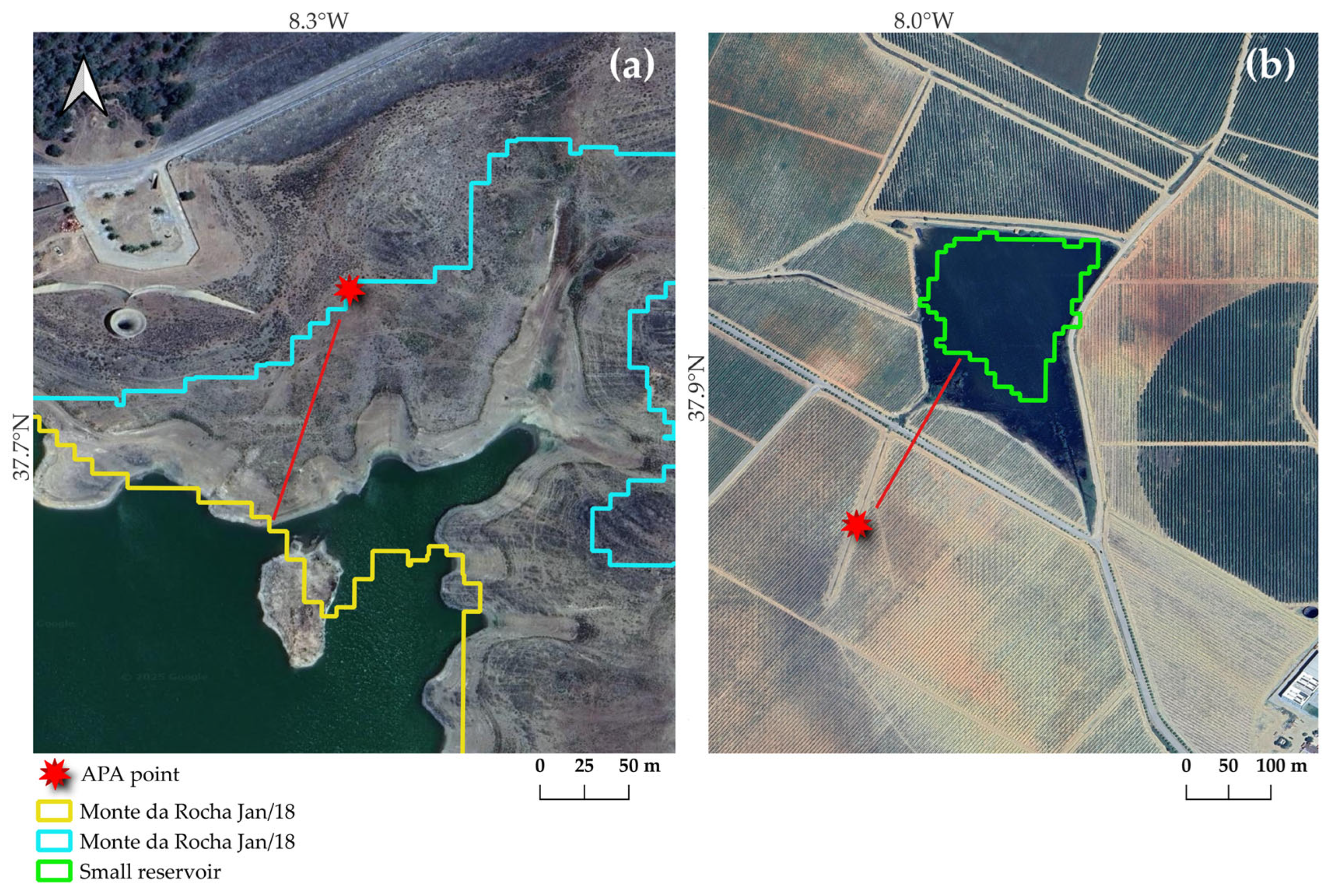
The method performance for identifying and locating small reservoirs was evaluated using 6370 georeferenced dam points, which were made available by the Portuguese Environment Agency (APA). Each point was associated with the closest polygons identified by the proposed method, using the “join attributes by location” processing tool of ArcGIS. A maximum distance of 150 m was established between the points and the closest detected polygon to account for potential variations in the flood area of small reservoirs (Figure 2b). This maximum distance was determined based on seasonal variations in the surface area of large reservoirs during the flood (represented by the blue polygon) and dry (represented by the yellow polygon) seasons (Figure 2a).

Since the data for small reservoirs monitored by APA do not have a specific collection date, and the polygons identified by the method correspond to the year 2023 at the end of the rainy season, when most reservoirs are assumed to be at their maximum level, some discrepancies may occur.

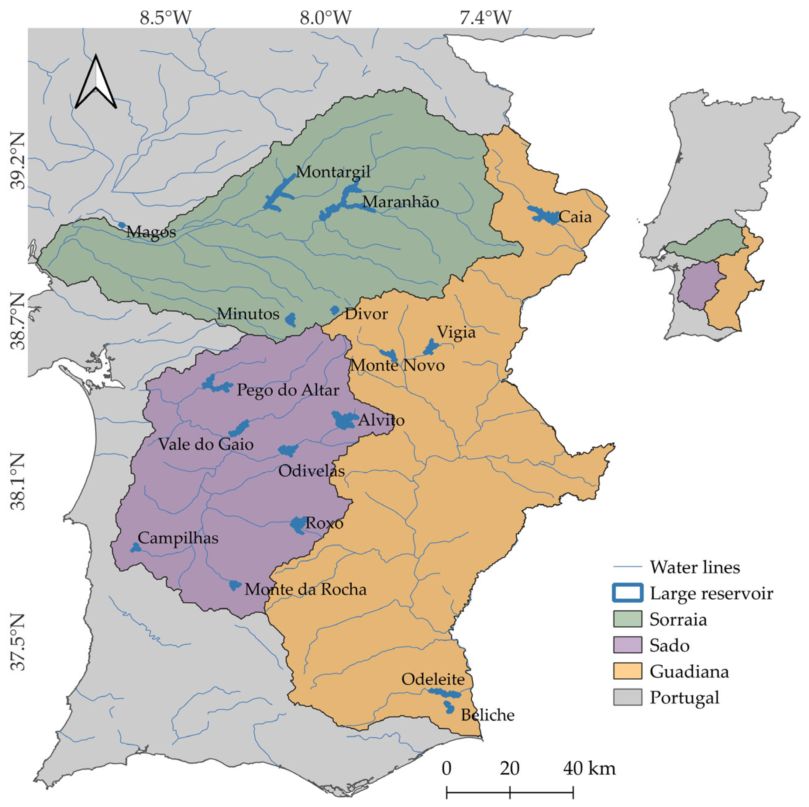
3. Case Study

This case study focuses on three semi-arid river basins in southern Portugal—Sorraia, Sado, and Guadiana—covering approximately 27,113 km². These basins contain numerous small private reservoirs, primarily built for irrigation, in addition to 17 major public reservoirs. The region experiences an average annual precipitation of 636 mm and evapotranspiration of 1337 mm [35]. According to the Köppen–Geiger classification the climate is categorized as Csa (Mediterranean/Continental), characterized by distinct seasons and limited rainfall (Figure 3). Agriculture is the predominant activity in the region, which faces significant challenges in water management and environmental conservation.

The Sorraia river basin, covering 7730 km², is the closest to Lisbon, Portugal’s capital and largest city. While it includes some residential and industrial areas, agriculture remains the dominant activity, with 16,000 ha dedicated to irrigated crops such as corn, rice, and tomatoes. This irrigation is primarily supported by the Montargil and Maranhão reservoirs [36]. The river basin has a median slope of 4%, with its highest point reaching 736 m.

The Guadiana river basin, shared with Spain and covering 67,174 km², with 11,600 km² located in Portugal. The river basin in Portugal has a median slope of 5%, with its highest point reaching 1018 m [37]. Traditionally reliant on rainfed agriculture, the region underwent a significant transformation with the construction of the Alqueva Multipurpose Project at the beginning of the 21st century—the largest investment ever made in the area. The Alqueva reservoir, with a total storage capacity of 4150 Mm³, serves as the primary water source, distributing water to several supporting reservoirs. Today, the Alqueva general irrigation system, comprising more than 72 dams, supplies water to approximately 150,000 ha of farmland. The region hosts a diverse range of crops, with olive groves, cereals, vineyards, dry fruits, and vegetables being the most predominant [38].

Changes in climate patterns, such as droughts, have been studied in the basin, emphasizing the importance of ecological flows for sustainable water resource management [39].

The Sado river basin, covering 7700 km², is one of the driest in Portugal. It has a median slope of 3%, with its highest point reaching 490 m. Aside from the major industrial hubs of Setúbal, its estuary, and the port of Sines, agriculture remains the dominant activity. Irrigation is supported by several dedicated reservoirs, supplemented by water transfers from the Alqueva reservoir in the Guadiana river basin [40].

Table 2. Main characteristics of reservoirs. Sistema Nacional de Informação de Recursos Hídricos. (Accessed on 5 March 2022 from https://snirh.apambiente.pt/).

Reservoirs	Main Use	Total Capacity (dam3)	Net Capacity (dam3)	Dead Storage Volume (dam3)	Full Reservoir Level (m)	Maximum Full Level (m)	Minimum Operating Level (m)	Inundation Area at Full Level (ha)
Alvito	Human supply	132,500	130,000	2500	197.5	198.55	172	1480
Beliche	Human supply	48,000	47,600	400	52	52.5	15	292
Caia	Irrigation	203,000	192,300	10,700	233.5	233.9	192.4	1970
Campilhas	Irrigation	27,156	26,156	1000	108	109.15	92.53	333
Divor	Irrigation	11,900	11,890	10	261.4	262.2	249.5	265
Magos	Irrigation	3384	2852	180	16.68	16.78	10.4	124
Maranhão	Irrigation	205,400	180,900	24,500	130	130.13	85.47	1960
Minutos	Irrigation	52,000	47,400	2100	264	265.5	245	530
Montargil	Irrigation	164,300	142,700	21,600	80	80.75	65.05	1495
Mte da Rocha	Human supply	102,760	97,760	5000	137	138.45	113.25	1100
Monte Novo	Various	15,277	14,780	500	196	196.8	183.5	277.4
Odeleite	Irrigation	130,000	117,000	13,000	52	52.9	22	720
Odivelas	Irrigation	96,000	70,000	26,000	103	104.55	91.3	973
Pego do Altar	Irrigation	94,000	93,600	400	52.26	52.26	15	655
Roxo	Irrigation	96,312	89,512	6800	136	137	122	1378
Vale do Gaio	Irrigation	63,000	63,000	0	40.5	42.5	11	550
Vigia	Human supply	16,725	15,579	1146	224	224.75	210	262

lists the seventeen main reservoirs in the study area selected for validating the proposed method, along with their key characteristics. The Alqueva reservoir was excluded due to its vast surface area (250 km²), which extends into Spain.

The Portuguese Environment Agency (APA) maintains a register that documents the location of 6370 dams of different sizes in the study area, including the previously mentioned dams in accordance with Decree-Law No. 21/2018 [41]. This registry classifies the dams according to the Dam Safety Regulation and the Small Dams Regulation, which define six classes based on height, measured from the lowest foundation level to the dam crest, and reservoir level:

Class I or large dams: Dams with a height from the foundation to the crest above of 15 m or with a height above 10 m and a capacity exceeding 1 million cubic meters (hm³).

Class II dams: Dams with a height above 10 m, not included in the previous category.

Class III dams: Dams with a height between 5 and 10 m.

Class IV dams: Dams with a height between 2 and 5 m.

Class V dams: Dams with a height above 2 m, but with unknown accurate height information.

Class VI dams: Dams with a height less than 2 m.

Figure 4 presents the distribution of dams across these classes and

Table 3. Number of dams of each class per river basin.

Class/River Basin	Sorraia	Sado	Guadiana	Total
I	29	25	48	102
II	55	40	49	144
III	67	61	289	417
IV	16	72	623	711
V	987	88	109	1184
VI	40	966	2806	3812
Total	1194	1252	3924	6370

the number of dams of each class per river basin. It is important to note that APA acknowledges potential inaccuracies in the survey, particularly regarding the classification of smaller dams.

4. Results

4.1. Validation of the Water Extent of Large Reservoirs

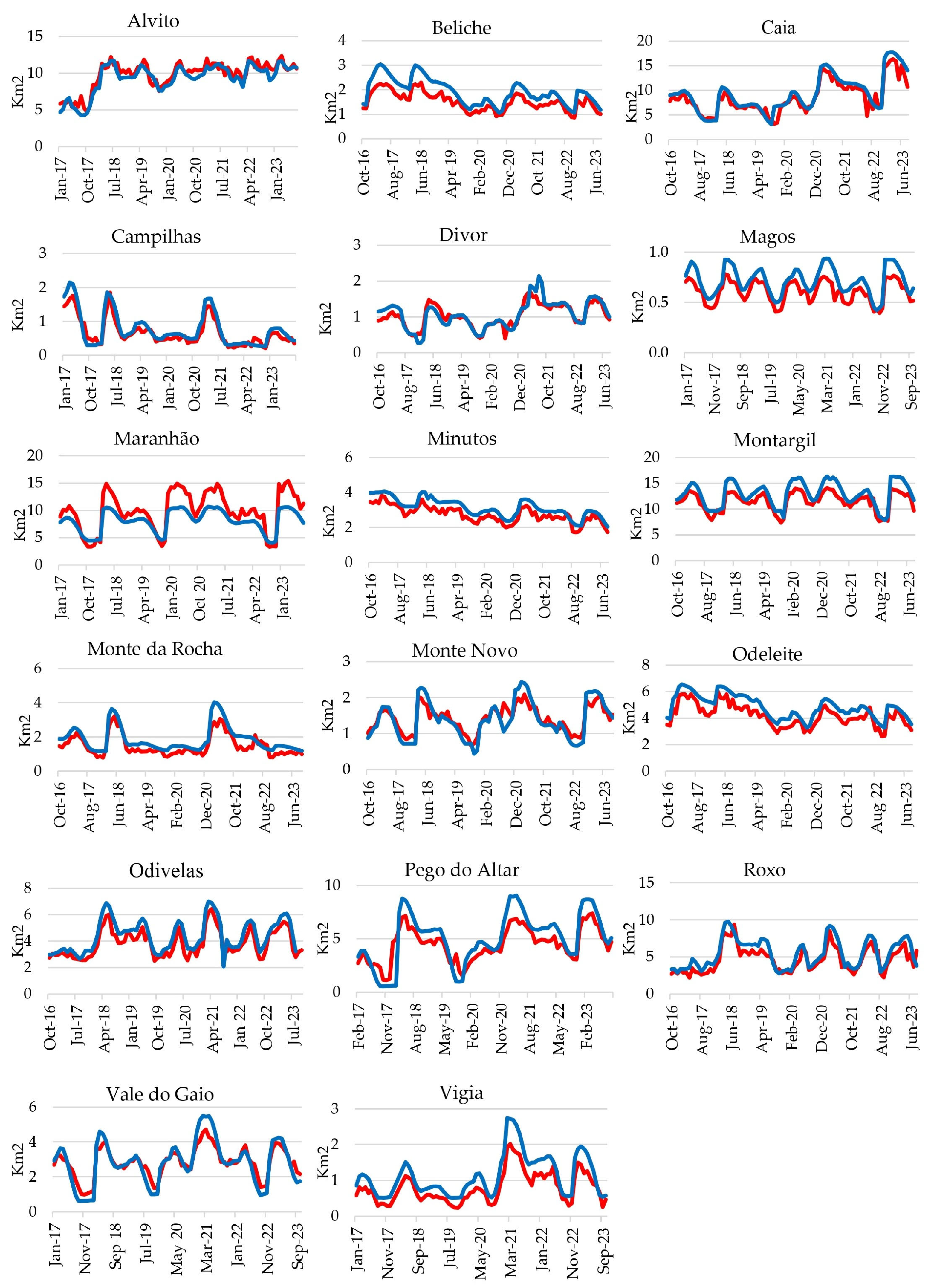
The evaluation of detection method performance was quantified differently for large public reservoirs and small private reservoirs. For large reservoirs, the assessment involved comparing the time series of detected surface areas with observed surface areas.

Figure 5 compares the observed and detected water surface areas across all 17 large reservoirs. Both datasets consistently exhibit the same seasonal patterns, with detected values closely matching the observed data in most reservoirs. However, the method’s performance declines in a few cases, notably the Beliche, Magos, Maranhão, Pego do Altar, and Vigia reservoirs. Additionally, the method generally appears to slightly underestimate the SNIRH values, except for the Alvito reservoir.

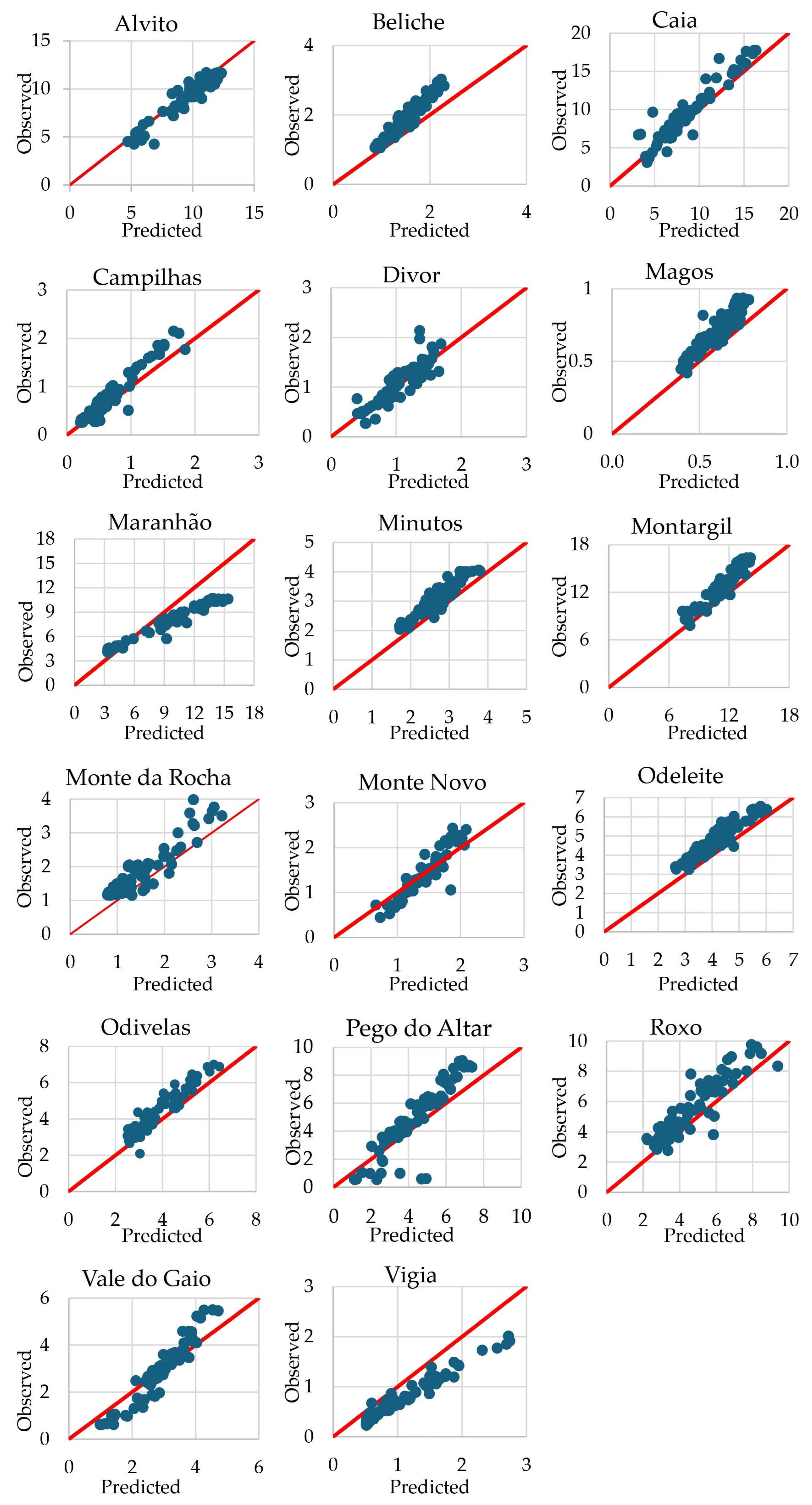
Figure 6 presents the correlation between the actual and detected surface areas. The small dispersion of points around the trend line reveals a strong correlation and further illustrates the good detection method performance. Among the 17 reservoirs, approximately 94% present an R² value above 0.82, 70% an RMSE value below 0.8, and 64% an NSE value above 0.5 (

Table 4. Statistics between observed and detected surface data, and statistics on terrain characteristics in each reservoir.

Reservoirs	R2	RMSE	PBIAS (%)	NSE	KGE
Alvito	0.89	0.78	4.98	0.84	0.87
Beliche	0.93	0.43	−20.29	0. 32	0.77
Caia	0.90	1.40	−8.08	0.86	0.77
Campilhas	0.93	0.19	−12.95	0.86	0.74
Divor	0.77	0.18	−2.71	0.76	0.75
Magos	0.84	0.12	−14.93	0.20	0.71
Maranhão	0.96	2.41	22.56	−0.43	0.70
Minutos	0.89	0.43	−12.43	0.32	0.94
Montargil	0.90	1.69	−11.38	0.45	0.83
Monte da Rocha	0.85	0.45	−18.74	0.62	0.83
Monte Novo	0.89	0.22	−0.60	0.79	0.67
Odeleite	0.89	0.71	−13.51	0.33	0.91
Odivelas	0.90	0.65	−12.40	0.68	0.80
Pego do Altar	0.82	1.32	−12.03	0.69	0.67
Roxo	0.84	1.09	−14.19	0.68	0.77
Vale do Gaio	0.93	0.48	0.07	0.85	0.70
Vigia	0.96	0.37	−29.17	0.58	0.63

).

The most robust performance was observed in the Alvito, Campilhas, Minutos, Monte Novo, and Vale do Gaio reservoirs, characterized by strong correlation coefficients (R > 0.89), low root mean square error (RMSE < 0.78), satisfactory percent bias (PBIAS: −12.95 to 4.98), and elevated Kling–Gupta efficiency (KGE > 0.70), consistent with well-calibrated results capable of replicating both temporal dynamics and magnitude ranges of observed data. Notably, the Minutos reservoir exhibited a relatively low Nash–Sutcliffe efficiency (NSE = 0.32) and pronounced negative bias (PBIAS = −12.95), yet achieved adequate KGE (0.94), suggesting partial alignment with observed variability despite underestimation. Monte Novo demonstrated balanced metrics (KGE = 0.67; PBIAS = −0.60), reflecting adequate accuracy alongside moderate representation of data variability.

The Caia, Divor, Odeleite, and Odivelas reservoirs displayed strong correlation indices (NSE > 0.77). However, Caia recorded high RMSE values (1.40), indicative of scatter in the detected area relative to observations. Odeleite and Odivelas exhibited significant percent bias (PBIAS > −12.40), highlighting underestimation despite successful replication of mean patterns and variability. Divor showed moderate KGE (0.75) and R² (0.77) combined with low PBIAS, suggesting minor dispersion effects in outputs.

Beliche, Montargil, and Monte da Rocha exhibited limited performance metrics (NSE < 0.45), underscoring detection inadequacies in reproducing observed patterns. Although Beliche demonstrated strong correlation (R = 0.93), low RMSE (0.43), and moderate KGE (0.77), its substantial negative bias (PBIAS = −20.29) points to significant underestimation, reflecting structural limitations in results for these reservoirs.

The Magos, Pego do Altar Roxo, and Vigia systems displayed pronounced percent bias (PBIAS > −12.03), indicating marked underestimation despite high coefficients of determination (R²). Suboptimal NSE (<0.69) and KGE (<0.77) values reinforce opportunities for parametric optimization and structural refinement.

The Maranhão reservoir demonstrated strong correlation (R = 0.96), but its substantial positive bias (PBIAS = 22.56) and inadequate variability capture suggest insufficient calibration, emphasizing the need for adjustments to address prediction errors in this reservoir.

4.2. Validation of the Water Extent Small Reservoirs

Table 5. Results for the reservoirs identified by APA (observed) and mapped by the proposed methodology (detected Reservoirs), described by classes of RSB and RPB.

Class	Observed	Detected Reservoirs
	Number	True Positive	False Negative	% of True Positives	Average Area (ha)	Median (ha)	Sum (ha)	Std. Dev. (ha)
I	102	99	3	97.06	125.07	35.09	12,382.0	277
II	144	127	17	88.19	12.36	5.98	1570.1	53.64
III	417	297	120	71.2	3.79	1.31	1125.2	9.46
IV	711	332	379	46.69	1.1	0.41	365.6	2.28
V	1184	916	268	77.36	2.59	1.16	2369.1	3.89
VI	3812	1453	2359	38.12	0.98	0.39	1420.8	2.03
TOTAL	6370	3224	3146	50.61	5.97	0.67	19,232.9	54.21

compares the number of reservoirs identified by the proposed method with the 6370 records provided by APA, distributed according to the six classes of the Dam Safety Regulation and the Small Dams Regulation. The table presents the number of reservoirs in the APA database that were correctly identified by the detection method (true positives), as well as those inaccurately identified or not identified at all (false negatives). The APA database contains 6370 records, of which 3224 were correctly identified. The proposed methodology suggests the existence of 7251 small reservoirs; however, 4027 of these are not listed in the APA database. Assuming the database is accurate, the number of false positives is 4027. Although the APA has records indicating the existence of these water bodies, the registration dates are not specified. Considering that small reservoirs can be perennial or temporary, depending on local climate conditions—and that they can also be deactivated or removed at the discretion of landowners—it is possible that, during the period covered by this study, the available information did not accurately reflect their current status.

Reviewing the results in greater detail, we observe a strong correlation between the number of reservoirs identified using the proposed methodology and the records in the database for classes I, II, and V, with a slightly weaker correspondence for class III (Figure 7). Notably, the number of reservoirs in class IV, which includes dams with heights between 2 and 5 m, is poorly detected, whereas the number of reservoirs in class V is better estimated. Since class V encompasses dams with heights exceeding 2 m but lacking precise height data, it can be inferred that most of these dams are likely over 5 m tall.

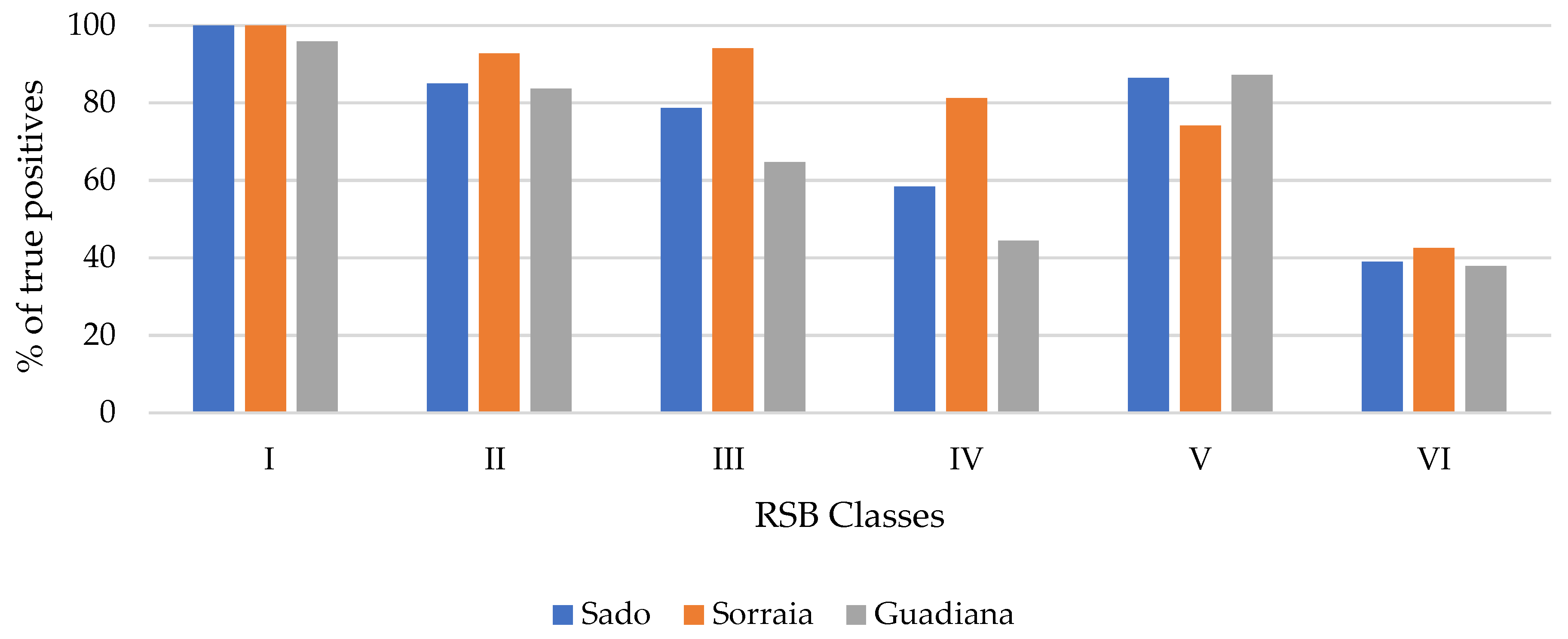
Figure 8 displays the percentage distribution of true positives per water quality class across the three analyzed river basins. The Sorraia river basin showed the highest percentages, while the Guadiana river basin recorded the lowest values. This discrepancy may be linked to methodological differences in monitoring practices by the Portuguese Environment Agency (APA), which implements distinct data collection protocols for each basin. Notably, in the Sorraia basin, Class IV exhibited a high rate of true positives despite containing the smallest number of monitored small reservoirs in this category (see quantitative details in Table 3).

From Table 5 results we can also infer that the proposed method performs well in identifying water bodies with areas above 10 ha (classes I and II) and reasonably well above 3 ha (classes II and V). Areas below 3 ha are poorly detected.

The procedure identified 7251 water bodies, of which 4027 were classified as reservoirs but remain unidentified in the APA database, representing false positives.

Table 6. Surface area statistics of unidentified detected polygons (false positives).

Classes Unidentified Small Reservoirs (ha)	n	Average Area (ha)	Median Areas (ha)	Sum (ha)	Sdt. Dev. (ha)
0.0–0.50	2594	0.2	0.2	530.9	0.1
0.50–1.29	979	0.8	0.8	787.6	0.2
1.29–2.68	328	1.8	1.7	586.8	0.4
2.68–4.97	77	3.6	3.5	275.2	0.7
4.97–9.35	42	6.5	6.2	271.8	1.2
9.35–19.04	7	14.9	14.3	104.2	3.5
TOTAL	4027	0.6	0.3	2556.6	1.1

describes the characteristics of these 4027 unidentified small reservoirs, distributed by six classes of surface areas generated using the natural breaks method (Jenks), which minimizes the variance within each class and maximizes the variance between classes. More than half of the false positives have surface areas of less than 1.8 ha.

Figure 9 shows some examples of non-identified water bodies (in green), with the recent background image from Google Earth. The images on the right are enlarged details from the left images.

5. Discussion

A large portion of the underestimation (reflected in negative PBIAS values) can be attributed to the use of the Gaussian filter integrated into the Otsu methodology. In this process, each pixel is replaced by a weighted average of its neighboring pixels, which smooths the edges and contours of the water bodies and consequently affects the land–water segmentation results. It is important to note that accurately delineating the boundaries between water and land is critical for precise segmentation in SAR images [42].

Another cause for the underestimation results may be related to the flat relief of the area. During periods of maximum water level, the geometry of the flooded area is more dynamic, including areas where the water depth is shallow. As the water extends over the relief, it mixes with vegetation, soil, and rocks. In SAR images, backscatter in the C band with VV polarization (C-VV) can be affected by complex terrain interactions [43]. In this scenario the increase in pixels backscatter hide the presence of water. In addition, confusion between sand and water is a common cause of detection failures in radar data.

Tan et al. (2023) [20], when evaluating the accuracy of the Otsu algorithm on Sentinel-1 images, found inconsistencies in the classification due to noise, with pixels showing a low backscatter coefficient in the terrestrial region and a high backscatter coefficient in the aquatic region. Misclassifications can cause other errors due to salt and pepper noise, which is often present in some SAR images, resulting in water areas classified as non-aquatic.

Zhang et al. (2022) [44] also observed that SAR image pixels with VV polarization are sensitive to variations in surface water depth in areas with sparse herbaceous vegetation. In this scenario, the pixel backscatter increases, hiding the presence of water. Peña-Luque et al. (2021) [45] also noted that the underestimation of the area detected during flood periods can be attributed to the dense vegetation that often covers the seasonally flooded banks and upstream areas of reservoirs. In addition, confusion between sand and water is a common cause of detection failures in radar data.

In addition, classical methods such as Otsu, although widely used for flood mapping, have important limitations in heterogeneous environments. As it uses a single threshold for segmentation, it is particularly susceptible to classification errors in areas with rugged terrain or terrain shadows, erroneously identifying regions as permanent or temporary water bodies [46].

The variability of the results can be attributed to the cutoff of the reservoir area based on the NWDI Index. The buffer was defined after several attempts, aiming to facilitate cropping for the largest possible set of SAR images. To fulfill the premise of Otsu’s method, the image cropped by the buffer must present a pixel frequency histogram with a bimodal distribution. However, the cut-off, based on the three different peak rainfall phases for each hydrological year (Table 1), may not adequately account for variations in the expansion and contraction of the water area in each month. Furthermore, defining a buffer of 100 m from the banks may not be adequate to adjust for the different flood areas in each reservoir.

In cases where the detection methods for these reservoirs were inadequately calibrated and the results failed to effectively capture data variability, the expected bimodal distribution was not observed in many of the SAR images. This shortcoming led to inaccurate segmentations over several months. Similarly, ref. [47] reported classification errors and minor omissions in surface area in images that did not conform to the bimodal distribution hypothesis.

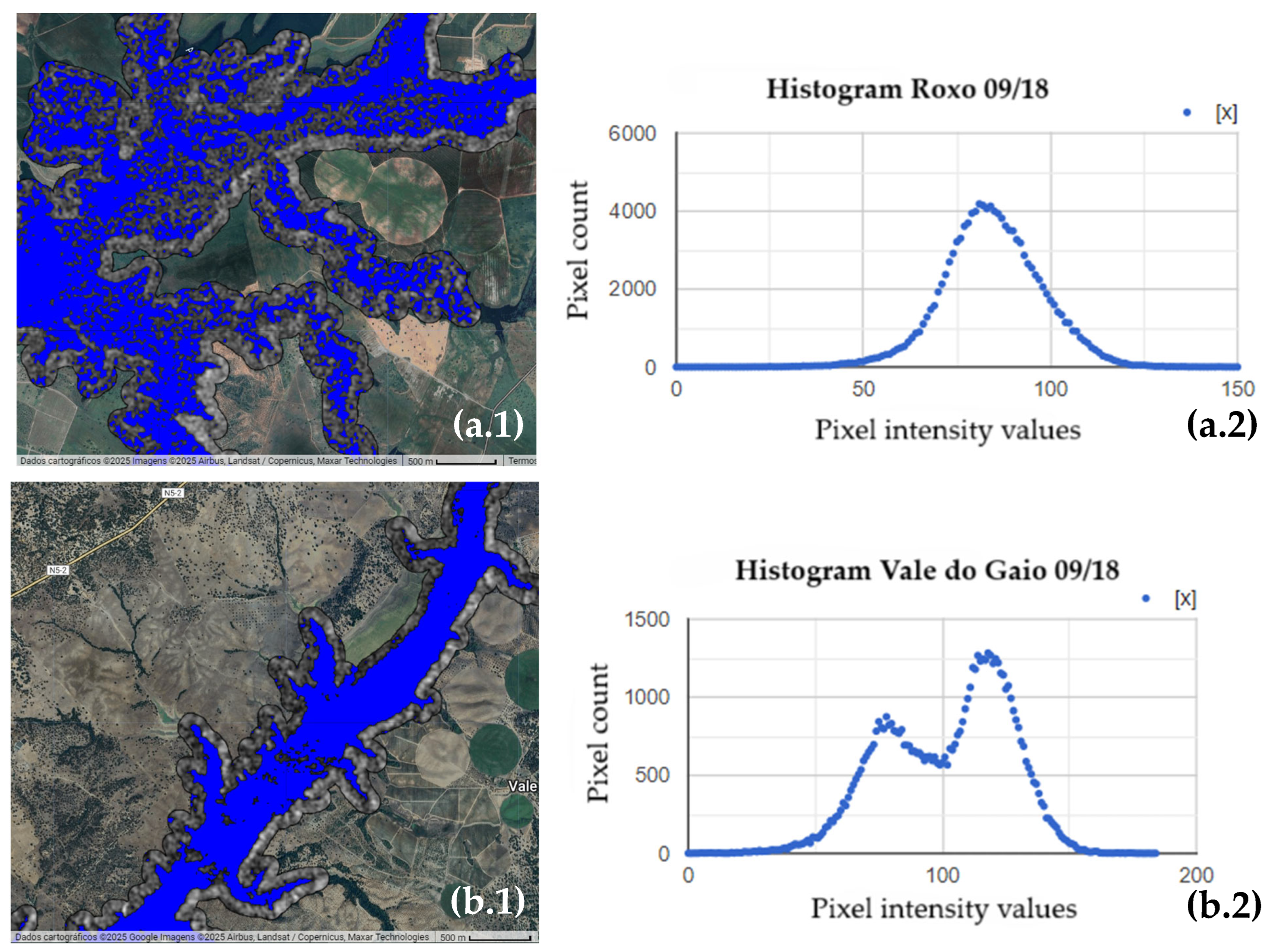
The results for Roxo and Vale do Gaio came from the same SAR image. For the Vale do Gaio reservoir, with a correlation of 0.92 and PBIAS of 0.07, the buffer clipping area was adequate. However, the lower NSE of Roxo at 0.68 and its PBIAS of −14.19 indicates that further adjustments should be made to the initial buffer to ensure a SAR image with a bimodal distribution. In the Roxo reservoir (a.1) the value did not guarantee the bimodal assumption as required by the OTSU method (a.2), resulting in inaccuracies in the delineation of the water extent, as evidenced by the Otsu-derived mask presenting internal voids and speckled patterns indicative of segmentation noise and misclassification. In contrast, for the Vale do Gaio reservoir the clipping area exhibited a clear bimodal distribution (b.2), and the Otsu-derived mask showed coherent boundaries and a continuous surface (b.1), leading to accurate water extent mapping(Figure 10).

Errors in the identification of small reservoirs may originate from multiple sources, with the primary inaccuracies stemming from the reference database of the Portuguese Environment Agency (APA), as acknowledged by the institution. The analysis, based on orbital images from March 2023, reveals that the absence of temporal metadata in the APA database—such as precise collection dates—introduces discrepancies attributable to chronological incompatibilities. Additionally, the high number of unidentified polygons in the territory (Table 6) suggests the existence of recent, unmonitored reservoirs, exacerbating mapping gaps.

These challenges are intensified by the intermittent nature of small reservoirs, whose surface presence varies seasonally in response to water balance components, such as precipitation and reservoir evaporation.

Most of the reviewed articles focus on larger reservoirs, while this study made specific adaptations to investigate very small reservoirs whose areas range from 0.2 to 1 ha and which still lack adequate validation. Several studies have addressed the mapping and validation of reservoirs around 10 ha. For instance, Wu et al. (2023) [48] used deep learning techniques and Sentinel satellite imagery on four reservoirs to estimate water levels.

This gap becomes even more relevant according to Búrquez, A. et al. (2024) [49]. Small reservoirs, averaging 0.5 ha, have a significant impact on the hydrology and connectivity of river basins, being able to disconnect up to 33% of the basin area and substantially modify water and sediment fluxes. Mady et al. (2020) [50], who identified evaporative losses of up to 38% of the volume in reservoirs with less than 10 ha during the dry season, and by Donchyts et al. (2022) [51], who demonstrated significantly greater inter-annual and intra-annual variability in reservoirs with less than 100 ha, using the Otsu method. The direct relationship between surface area and volume in shallow reservoirs [52] also enhances abrupt changes in the surface associated with evaporation or climate variability, affecting the accuracy of remote sensing techniques.

In view of this, the need to deepen the mapping and validation in reservoirs of reduced dimensions and not yet monitored is reinforced to ensure the development of more robust and accurate methods for monitoring these structures over time. Furthermore, the margins of these reservoirs exhibit critical phenological alterations—such as shallow-water zones, sparse vegetation (shrubs and small trees), and sandy areas—that reduce SAR signal sensitivity, complicating the precise delineation of water bodies compared to optical data [44,45].

Given this scenario, the implementation of validation methods and long-term temporal studies is imperative to monitor the dynamics of these reservoirs and discriminate those that persist in the territory. This approach is essential to update reference databases, increase the accuracy of detection methods, and assist hydrological models at local and regional scales.

Despite the limitations of the Otsu method, especially in areas with vegetation and moist soils, as well as the dependence on bimodal histograms and global thresholds, they highlight the need for more flexible and adaptive approaches for reservoir mapping. In this context, the method adopted in this study seeks to overcome these restrictions by considering the spatiotemporal specificities of each reservoir and allowing adjustments in the buffer size parameters according to the observed environmental conditions. In this way, it is possible to minimize the influence of noise, shadows, dense vegetation, and seasonal variations on the dynamics of flood areas, providing a more accurate and reliable delimitation. Furthermore, the validation of the results with complementary data reinforces the robustness of the method and its applicability in different scenarios and reservoir formats.

6. Conclusions

Advances in remote sensing techniques for water bodies, using images from the Sentinel-1 and Sentinel-2 satellites, have been widely used in various scientific studies. However, the validation of this information with data collected in situ is still limited. This study developed an automatic algorithm on the GEE platform for mapping the surface area of large and small reservoirs, subsequently validating it with in situ data from the Portuguese Environment Agency (APA).

Combining optical and radar images allows water to be detected using consolidated methods such as the NDWI and the Otsu image thresholding technique. Given the susceptibility of optical images to cloud cover, a complementary approach was applied using SAR images.

The detected data were validated in two different ways. In the first stage, the surface area results of the large reservoirs were validated with real surface areas defined by water authority equations. The correlation graphs between the observed area and the detected area showed significant adherence in 14 of the 17 reservoirs, indicating satisfactory accuracy (R² > 0.82). Inter-annual underestimation was also observed in 16 reservoirs, attributed to the Gaussian filtering of the Otsu method, which smooths edges and contours, and the difficulty of identifying water pixels in shallow regions or with herbaceous vegetation in SAR images. This segmentation can result in incorrect classifications on the banks of reservoirs, especially during periods of flooding.

In the second stage, the methodology focused on the small reservoirs in the study area in an image from March 2023, to identify the small reservoirs registered with the water authorities. The method showed promising results in identifying reservoirs with an elevation above 5 m and, according to the detected data, an average area of 3 ha. However, it had limited performance in detecting smaller reservoirs due to the difficulty of identifying pixels in areas with shallow depths and aquatic vegetation. Accuracy in detecting small reservoirs is complex due to the variability of rainfall and temperature [50,51,52], making it difficult to monitor them over the long term. Despite the satisfactory validation of the method, some aspects need to be improved. The Otsu technique is accurate when the histogram of the pixels in the image follows the bimodal premise. The algorithm should be developed to allow for more precise adjustments to the clipping limits of SAR images, considering different seasons and specific reservoirs. The error can be minimized for detailed results by overlaying vegetation indices, adjusting the salt and pepper noise of SAR images, using digital terrain models and altimetry data, and ensuring that shallow water pixels and vegetated banks are correctly classified as water pixels in the final result.

This methodology allows for the identification and monitoring of reservoirs that are not yet registered by the regulatory authorities. The use of this approach can contribute to the identification of newly built, intermittent, and decommissioned reservoirs and those most susceptible to drought, supporting management and enforcement processes.