Distinct Regional and Seasonal Patterns of Atmospheric NH₃ Observed from Satellite over East Asia

Abstract

Ammonia (NH₃), as a vital component of the nitrogen cycle, exerts significant influence on the biosphere, air quality, and climate by contributing to secondary aerosol formation through its reactions with sulfur dioxide (SO₂) and nitrogen oxides (NO_x). Despite its critical environmental role, NH₃’s transient atmospheric lifetime and the variability in spatial and temporal distributions pose challenges for effective global monitoring and comprehensive impact assessment. Recognizing the inadequacies in current in situ measurement capabilities, this study embarked on an extensive analysis of NH₃’s temporal and spatial characteristics over East Asia, using the Infrared Atmospheric Sounding Interferometer (IASI) onboard the MetOp-B satellite from 2013 to 2024. The atmospheric NH₃ concentrations exhibit clear seasonality, beginning to rise in spring, peaking in summer, and then decreasing in winter. Overall, atmospheric NH₃ shows an annual increasing trend, with significant increases particularly evident in Eastern China, especially in June. The regional NH₃ trends within China have varied, with steady increases across most regions, while the Northeastern China Plain remained stable until a recent rapid rise. South Korea continues to show consistent and accelerating growth. East Asia demonstrates similar NH₃ emission characteristics, driven by farmland and livestock. The spatial and temporal inconsistencies between satellite data and global chemical transport models underscore the importance of establishing accurate NH₃ emission inventories in East Asia.

1. Introduction

Ammonia (NH₃) is a primary pollutant directly emitted into the atmosphere. Emissions of NH₃ into the atmosphere are mainly caused by agricultural activities such as fertilizers and volatilization of agricultural waste, and livestock [1,2,3], and are also emitted by anthropogenic fossil fuel combustion, biomass burning, and industry [1,4,5]. The emitted NH₃ act as an important precursor by reacting with sulfur dioxide (SO₂) and nitrogen oxides (NO_x) in the atmosphere to form ammonium sulfate ((NH₄)₂SO₄) and ammonium nitrate (NH₄NO₃), which become the main components of secondary particulate matter and plays a crucial role in aerosol formation [6]. Furthermore, NH₃, which is linked to the nitrogen cycle, has an impact on the biosphere as well as air quality and climate [7,8].

The atmospheric concentrations of NH₃, which have a relatively short lifetime ranging from hours to days (typically within 24 h) [9,10,11], are liable to change in both spatial and temporal terms. Therefore, high concentrations of NH₃ can be observed around the emission source because it deposits or reacts as time passes and distance increases from the source location. For this reason, it needs to understand the abundance of NH₃ in the atmosphere and its spatiotemporal variation. Despite the growing importance of NH₃ monitoring, observations of spatiotemporal variability in NH₃ are limited, owing to measurement difficulties. In situ measurement networks are extremely rare and have a limited ability to monitor global coverage. Satellites with a wide spatial range are useful for identifying the NH₃ concentration distribution and seasonal variability by continuously providing information on areas that cannot be covered by ground-based observations. Recently, many studies that noted NH₃ retrieval from the infrared spectrum observed it from various satellites (e.g., AIRS, Atmospheric Infrared Sounder [12], and IASI, Infrared Atmospheric Interferometer [13,14]) and this has been actively shown [15,16].

It has been established that China, Russia, and India significantly contribute to global NH₃ emissions. These studies were predominantly performed with countries scaled on the U.S. or Europe that focused on large point sources, and a commonly high resolution NH₃ spatial distribution map based on satellite data had been reported as an annual interval. In addition, there is a significant discrepancy between NH₃ observations and predicted values derived from the chemical transport models (CTMs), which applied bottom-up inventories [17]. This large uncertainty in NH₃ emission inventories is due to the lack of measurements and difficulty in formulating representative emission factors for each local region with regard to the various source sectors. Also, the large point sources that were unrevealed from the bottom-up inventory were detected by satellite observation [18]. Previous studies on NH₃ have typically been conducted over relatively short periods [19,20,21] or focused on localized specific regions [20]. In cases where analysis spans over ten years or more, studies have usually been conducted at continental scales [22]. The research on the atmospheric NH₃ in East Asia has primarily focused on China, which is well-known as a major emission source region. In particular, the long-term analyses specifically addressing Japan and the Korean Peninsula remain notably scarce, underscoring the critical need for detailed investigations in these regions.

Therefore, in this study, we not only identify long-term trends and seasonal variability but also pinpoint regions with similar emission characteristics in East Asia using satellite observations. In Section 2, we described the satellite and CTM dataset. Section 3 describes the spatial distribution characteristics and annual/seasonal variability of NH₃ concentration in East Asia, and classifies areas showing the same emission characteristics. Additionally, we show the intercomparison results between satellite observations and CTM-simulated NH₃ concentrations over East Asia.

2. Satellite and Chemical Transport Model Data

2.1. IASI NH₃

The IASI, a sensor that monitors for atmospheric sounding and composition observations, onboard the MetOp series (MetOp A, B, and C which were launched in 2006, 2012, and 2018, respectively), is operated by the European Organization for the Exploitation of Meteorological Satellites (EUMETSAT). The IASI measures infrared radiation at top-of-atmosphere (TOA), which is emitted by the Earth’s atmosphere from 645 to 2760 cm⁻¹ with a high spectral resolution of 0.25 cm⁻¹. The IASI is widely used in various studies, such as identifying trends and variability in atmospheric composition and evaluating climate models as well as assimilation of the atmospheric thermodynamic profiles on numerical weather prediction models [23,24].

The NH₃ total column concentration data retrieved from IASI/MetOp-B (ANNI-NH3-v4.0.0 [25]) were obtained from 2013 to 2024. This level 2 NH₃ total column in a near-real-time dataset from IASI observation was generated by the Université Libre de Bruxelles (ULB), Belgium. The IASI overpasses through the local area twice a day (morning and evening), but we only used data from the morning time (~09:30 LST) because the thermal contrast is better compared to that of the evening [26]. To ensure clean pixels uncontaminated by clouds, we used cloud filtering criteria (cloud cover < 10%) in other studies [27,28]. In addition, to minimize the influence of retrieval and measurement errors, only pixels flagged as good (quality flag = 1; recommended) in both the pre-filtering and post-retrieval quality control steps were selected. These selected pixels were subsequently oversampled onto 0.25° × 0.25° grid (approximately 20–25 km horizontal resolution at mid-latitudes).

2.2. CAM-Chem

The CAM-chem is a part of the National Center for Atmospheric Research (NCAR) Community Earth System Model (CESM) and is utilized for simulations of global tropospheric and stratospheric atmospheric composition. Its simulation output is used also as boundary conditions for regional modeling [29] and available for 1 January 2001 at 6 h intervals. Its domain has a 0.9° × 1.25° horizontal resolution and 56 vertical levels (sigma hybrid coordinates) [30]. Meteorology in the CAM-chem is driven by specified dynamics, by nudging with 50 h relaxation (1%) to Modern-Era Retrospective analysis for Research and Applications, version 2 (MERRA2) reanalysis.

Chemistry in the CAM-chem is used for the Model for OZone And Related chemical Tracers–Tropospheric chemistry scheme (MOZART–T1) mechanism, remarkably updated tropospheric chemistry from the MOZART mechanism [31]. Modal Aerosol Model with 4 modes—Volatility Basis Set (MAM4–VBS) scheme is used for aerosols including secondary organic aerosols [32,33].

For anthropogenic emissions, the CAMS-GLOB-ANT_V2.1 (Copernicus Atmosphere Monitoring Service, the 2000–2019 global anthropogenic emissions), which is based on the Emission Database for Global Atmospheric Research (EDGARv4.3.2) inventory [34] and the Community Emissions Data System (CEDS) emissions [35], is used. Biogenic emissions are from Model of Emissions of Gases and Aerosols from Nature (MEGAN2.1 [36,37]). Fire emissions are used by multiplying CO₂ from Quick Fire Emissions Dataset (QFED) as the base inventory by the Fire INventory for NCAR (FINN) emission ratios [38].

2.3. CAMS

The CAMS reanalysis (CAMSRA) is a global reanalysis dataset of atmospheric composition produced by the European Centre for Medium-Range Weather Forecasts (ECMWF), a three-dimensional atmospheric composition field including aerosols and chemical species [39]. It has covered a temporal resolution of 3 h since 2003. Its domain has approximately 80 km (0.7° × 0.7° grid) horizontal resolution and 60 hybrid sigma-pressure levels vertical resolution. It was generated by assimilating satellite retrievals of CO, NO₂, O₃, and Aerosol Optical Depth (AOD) from multiple sensors with ECMWF’s Integrated Forecast System (IFS). The chemical mechanism of the IFS is an improved version of the Carbon Bond 2005 chemistry scheme (CB05) [40] for the troposphere with an implementation of the CTM Transport Model 5 (TM5) [41]. Anthropogenic emissions were from the MACCity inventory [42] and biogenic emissions were calculated by the MEGAN2.1 model that used meteorological fields from the MERRA2 reanalysis following [43]. In addition, biomass burning emissions were provided by the Global Fire Assimilation System, version 1.2 (GFASv1.2) [44].

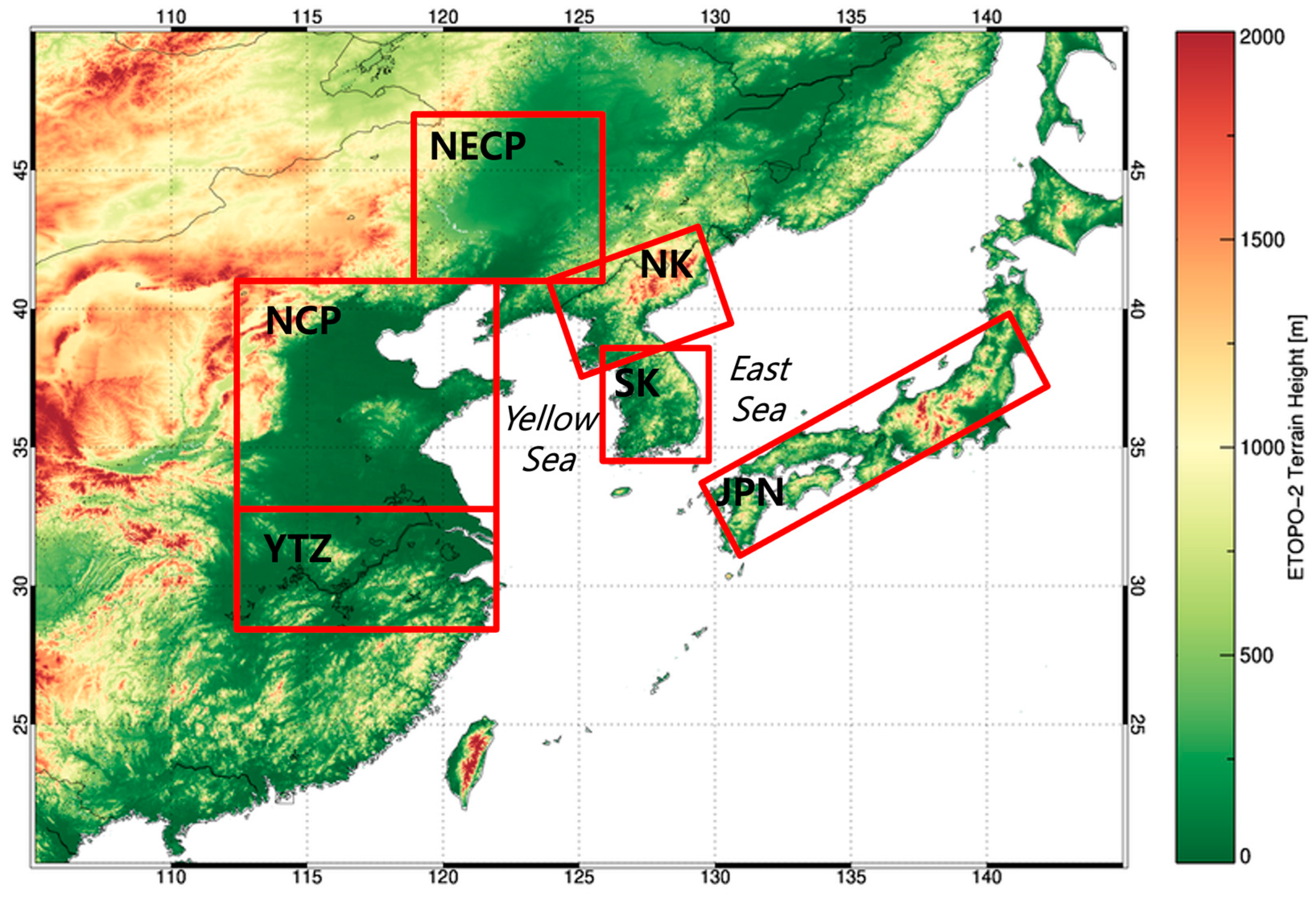
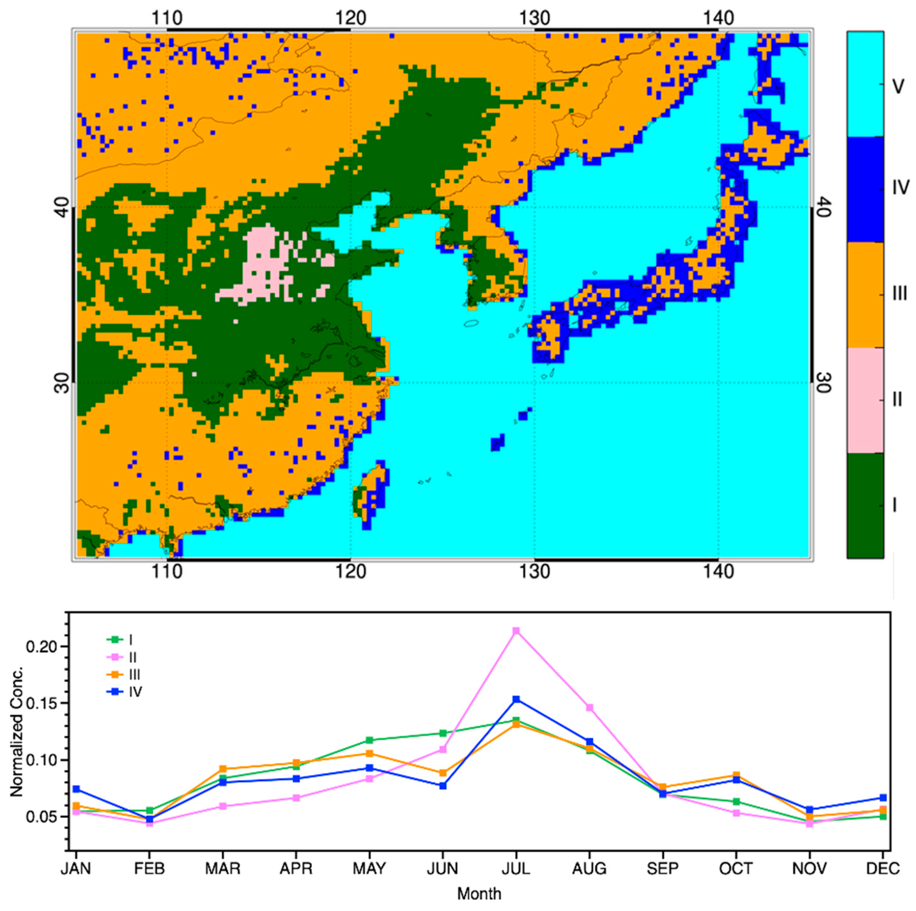
2.4. Region Selection

To evaluate the spatiotemporal variability of NH₃ concentration at a regional scale with an emphasis on East Asia (105–145°E, 20–50°N), including not only China, a major NH₃ emitting nation, but also the Korean peninsula and Japan, we divided the major regions of interest into six regions (NECP; North Eastern China Plain, NCP; North China Plain, YTZ; Yangtze Plain, NK; North Korea, SK; South Korea, JPN; Japan) and compared the volatility of averaged concentrations in each region (Figure 1). Later, we focus on this area of interest, analyzing and comparing satellite and model results about the magnitude of concentrations and seasonality. To quantitatively compare satellite-derived NH₃ concentrations with model results (CAM-Chem and CAMS), we calculated monthly averaged NH₃ column concentrations within each region of interest by averaging all valid pixels falling within the corresponding regional boundaries.

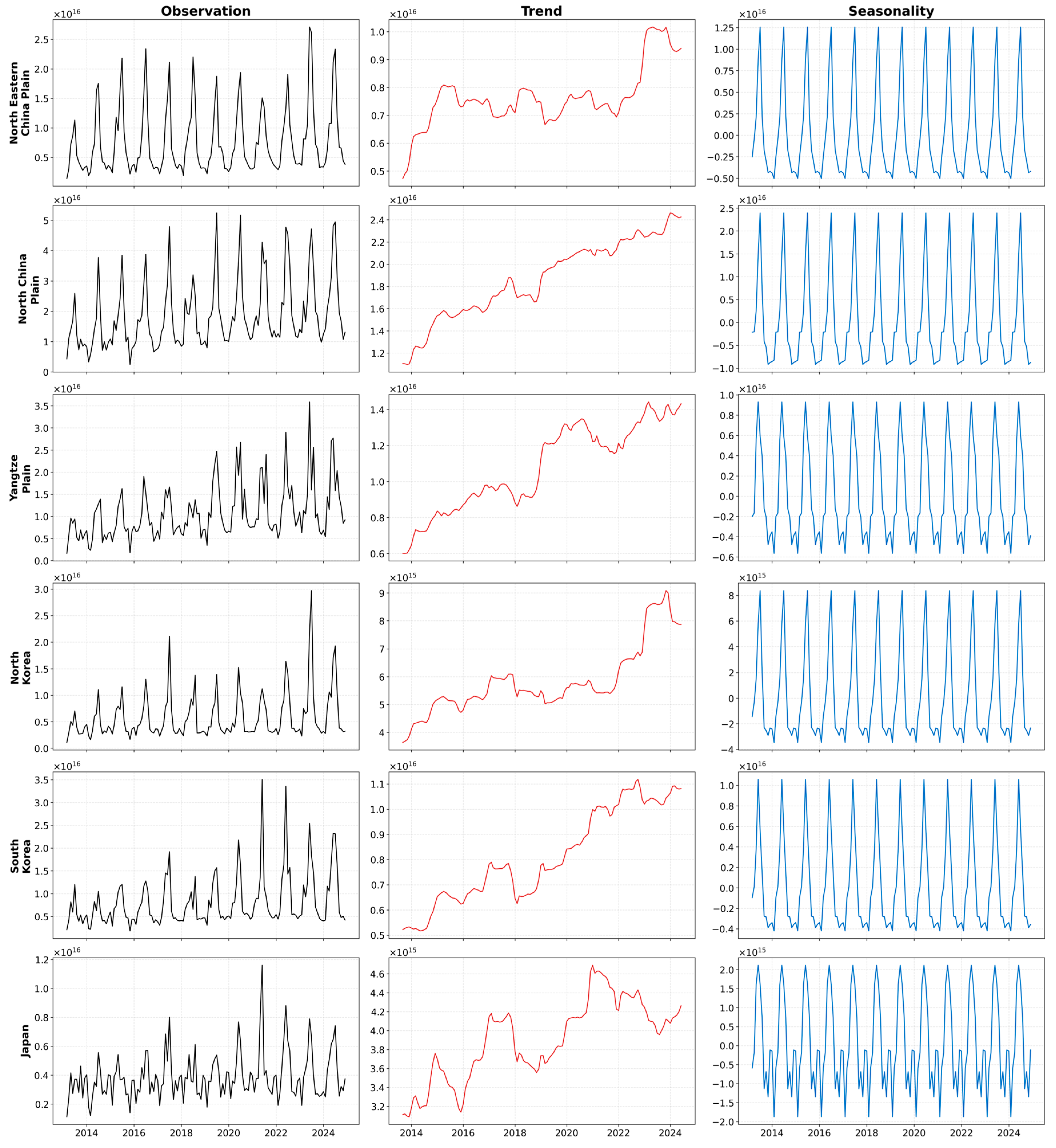
2.5. Time Series Decomposition Analysis

To identify the temporal variability and long-term trends of NH₃ concentrations in each interest region where high concentrations are observed, we performed a time series decomposition analysis for each interest regions that determined in Figure 1 as the following equation:

$$Y_t=S_t+T_t+R_t$$

(1)

where Y_t is the observed NH₃ concentration. S_t, T_t, R_t are the seasonal-cycle component, trend component, and residual component, respectively. The subscript t represents the function of the observation time. S_t represents the recurring variations that follow a consistent annual cycle. In cases where major NH₃ emission activities, such as those related to agriculture and livestock farming, are concentrated in specific seasons, regular patterns become evident. We applied the additive decomposition method, which assumes a constant seasonal amplitude over the entire period. The annual seasonal amplitude ($A_y$) for each year was calculated from the S_t as follows:

$$A_y=\underset{\mathrm{t}\in \mathrm{y}}{\max }\left(S_t\right)-\underset{\mathrm{t}\in \mathrm{y}}{\min }\left(S_t\right)$$

(2)

where $\mathrm{t}\in \mathrm{y}$ represents all monthly points within the year. The coefficient of variation (CV) of the annual amplitude was calculated to quantify the year-to-year variation in seasonal amplitude.

$$CV(\%)={\displaystyle \frac{{\sigma }_A}{{\mu }_A}}\times 100$$

(3)

where ${\mu }_A$ and ${\sigma }_A$ represent the mean and standard deviation of annual amplitudes, respectively. The CV values ranged between 0 and 3.8% across all interest regions, indicating stable seasonal amplitudes during the analysis period.

T_t denotes the long-term and sustained trend in NH₃ concentrations. This component reflects the influence of long-term factors, such as changes in the characteristics of local emission sources, increases or decreases in emissions, and the effects of policy measures. R_t refers to the irregular and unpredictable fluctuations that remain after removing both the S_t and T_t components from the original observed time series. These variations are primarily caused by observational errors, short-term meteorological effects, and unforeseeable event.

3. Results

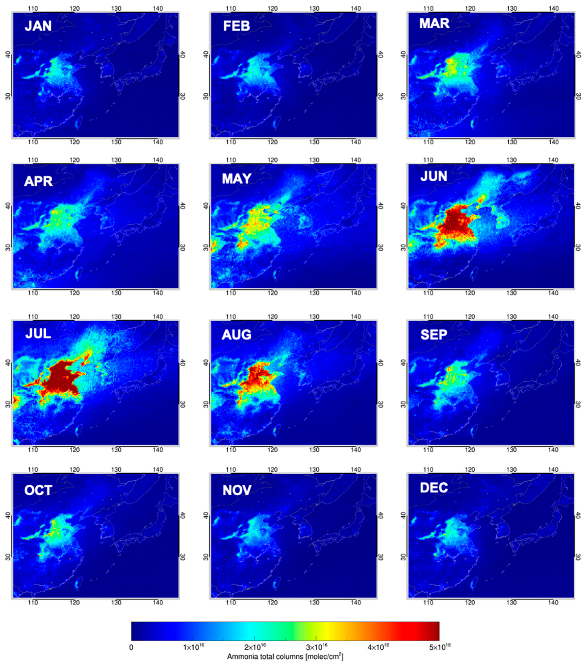
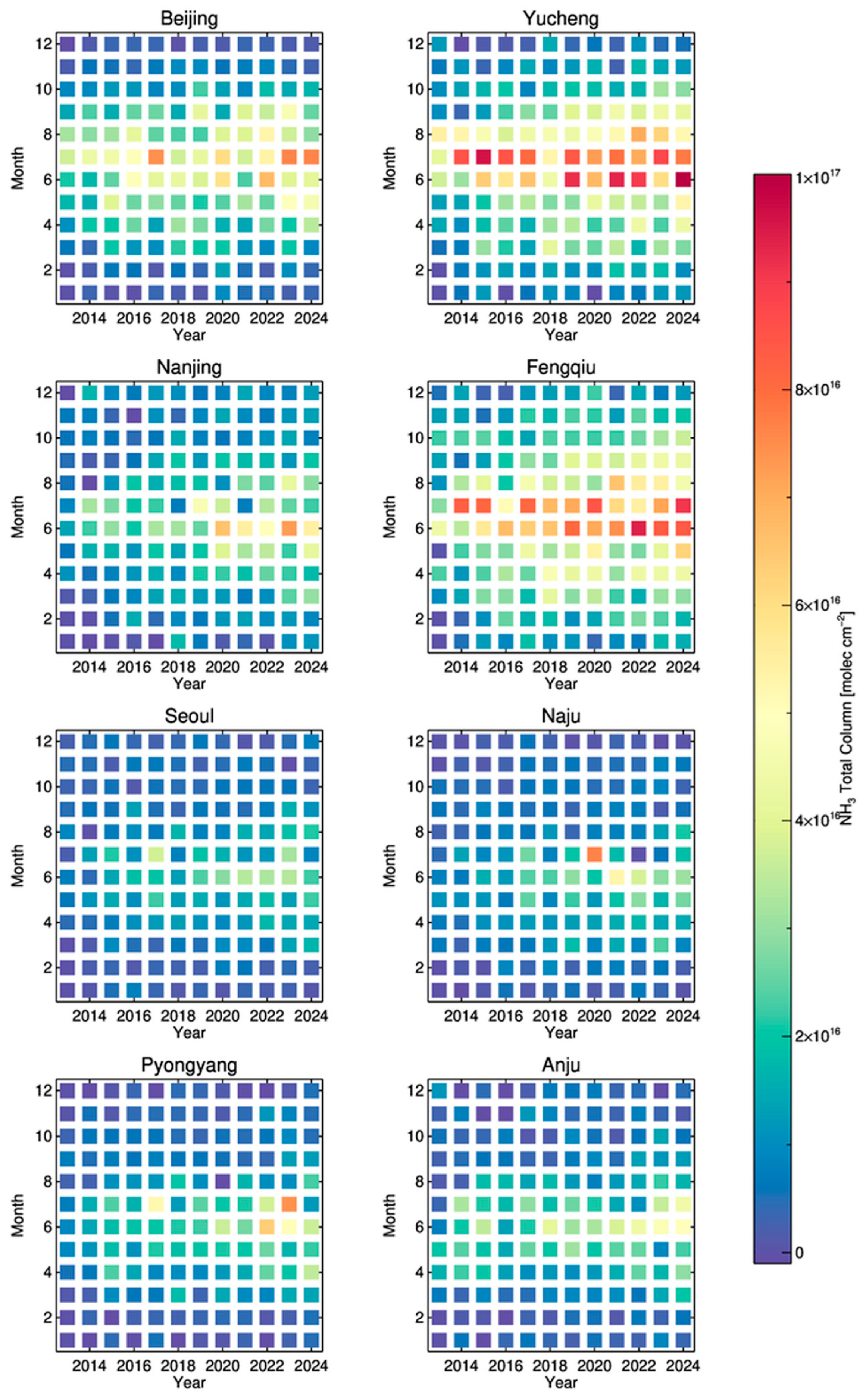
3.1. Spatiotemporal Distribution of NH₃

The spatial distribution of monthly averaged NH₃ total column concentration from the IASI for the period of 2013–2024 are shown in Figure 2. Clear seasonal variations and hotspot regions are evident in East Asia. Atmospheric NH₃ concentration due to NH₃ emissions is low in winter, begins to increase in spring starting in March, reaches a peak in summer (the highest peak value in July over North China Plain is about 1.0 × 10¹⁷ molecules cm⁻²), and then decreases. The influence of prominent emission regions of China is distinctly evident across all seasons. The region with the highest NH₃ concentration distribution in East Asia is China, followed by similar levels in North Korea and South Korea, with Japan having very low levels. In particular, regions with high NH₃ concentrations, such as North and South Korea, as well as the North China Plain and North Eastern China Plain, are clearly revealed in June and July. In this regard, the relatively high NH₃ concentration over the Yellow Sea and East Sea in summer compared to other seasons suggests that emitted NH₃ from mainland China may reach the Korean Peninsula across the sea due to long-range transport. In addition, elevated NH₃ concentrations observed in the southwestern Korean Peninsula during summer (June–July) are closely linked to agricultural regions with intensive rice cultivation. Furthermore, NH₃ levels in urban areas (e.g., Beijing, Nanjing) notably exceed those in Seoul, indicating stronger local industrial and transportation emissions.

Figure 3 shows the monthly variation in average NH₃ concentrations from 2013 to 2024 in representative major cities (Beijing (116.3°E, 39.9°N) and Nanjing (118.7°E, 32.1°N) in China; Seoul (126.9°E, 37.5°N) in South Korea; Pyeongyang (125.7°E, 39.0°N) in North Korea; farmlands (Yucheng (116.6°E, 37.0°N) and Fengqiu (114.6°E, 35.0°N) in China; Naju (126.7°E, 35.0°N) in South Korea; and Anju (125.6°E, 39.8°N) in North Korea in East Asia. These correspond to areas where major hotspots are observed in the spatial distribution of NH₃. In China, the NH₃ concentration is slightly higher (~130%) in farmlands (Yucheng and Fengqiu) in summer than in the large cities (Beijing and Nanjing). However, from a metropolitan perspective, on average, Beijing and Nanjing showed twice as high concentrations as Seoul and Pyeongyang. This demonstrates that large cities in China emit relatively higher levels of NH₃ into the atmosphere than other cities of countries, due to the influence of human activities and industry. On the other hand, in North and South Korea, NH₃ concentrations over plains and cities (the capital of each nation) are similar. Overall, it can be seen that the concentration in each region is increasing as the years go by, and the increasing trend is especially noticeable in the summer.

This increasing trend in NH₃ has also clearly occurred in the spatial distribution. Figure 4 shows the linear increase rate from 2013 to 2024 for each month. NH₃ tends to increase in all seasons, and the increase in concentration is more pronounced in summer, when NH₃ is abundant in the atmosphere. The concentration increase is most significant in June, particularly on the mainland of China where high levels are indicated in Figure 2. To objectively evaluate the statistical significance of these spatial trends, we performed additional analyses using p-values and t-statistics, as shown in Supplementary Figures S1 and S2. The lower p-values (≤0.05) highlight regions where the observed linear increases are statistically significant. Correspondingly, t-statistics represent the strength and robustness of these linear trends, with values exceeding 2.0 considered statistically significant at the 95% confidence level. Despite July having the highest NH₃ levels, the most notable increase occurs in June (maximum growth rate of 7.8 × 10¹⁵ molecules cm⁻² yr⁻¹). This likely reflects the combined effects of progressively warmer temperatures in early summer (June) and intensified agricultural activities and fertilizer use. In contrast, NH₃ concentrations in July remain consistently high, thus limiting further significant increases. Some areas (e.g., over Eastern China) exhibit a slight decreasing trend in July. However, this locally occurred spatial decreasing trend is in an area where the confidence level in July is relatively low (Figures S1 and S2). Furthermore, South Korea also shows a distinct increasing trend in June. As previously described, this increase is influenced by the long-range transport of high-concentration cases, which is also evident over the ocean.

Figure 5 show the observed values, trends, and seasonal results according to the time series decomposition for each region. In all regions, the seasonal cycle of increase in summer and decrease in winter that repeats every year was clearly generated. The amplitude of these seasonal fluctuations is more pronounced in areas with higher concentrations of atmospheric NH₃. Japan, where the NH₃ concentration levels are closer to background levels, exhibits weaker seasonality. As the distance increases from China, the primary source region of NH₃ emissions, the concentration of externally transported NH₃ correspondingly decreases. Consequently, seasonal variations in NH₃ concentration become less pronounced in Japan, where local emission sources are limited. Given the short atmospheric lifetime of NH₃, the clear decreasing gradient in NH₃ concentrations from China to South Korea and then to Japan provides another evidence that NH₃ undergoes significant removal during long-range transport.

The temporal variations in atmospheric NH₃ concentrations across East Asia, derived from time series decomposition analysis over the period 2014–2024, reveal clear regional contrasts. The North China Plain exhibited consistently high concentrations and the most robust upward trend throughout the decade, with its trend component nearly doubling, indicating persistent regional emission intensification. In contrast, the North Eastern China Plain maintained relatively stable NH₃ concentrations from approximately 2015 to 2022, followed by an abrupt increase of roughly 80%, distinctly different from trends in other regions of China. Similarly, the Yangtze River Plain generally showed continuous growth, experiencing only a brief and slight decline around 2021 before resuming an upward trend.

Both North and South Korea exhibited increasing NH₃ trends. North Korea experienced a rapid and marked increase in NH₃ concentrations after 2022, suggesting recent intensified emission activities. South Korea, on the other hand, showed a steady and accelerating increase over the entire study period, with the most pronounced growth occurring since the late 2010s. Notably, peak NH₃ concentrations in South Korea in June 2021 (~1.2 × 10¹⁵ molecules cm⁻²) were approximately threefold greater than those observed in June 2013 (~3.5 × 10¹⁵ molecules cm⁻²), highlighting significant changes in the regional atmospheric composition and potential implications for secondary aerosol formation. Japan exhibited relatively minor NH₃ concentration variations throughout the studied period, with concentrations consistently lower and stable compared to other East Asia regions.

To understand the patterns and characteristics of the East Asia region showing spatial and temporal variability of NH₃, we categorized them using the K-means clustering method. This unsupervised and non-deterministic iterative numerical method partitions data into multiple clusters to minimize inter-cluster similarity and maximize intra-cluster similarity. Figure 6 shows the classified maps based on NH₃ concentration and monthly variability through K-means method. It was classified into a total of five cluster categories, including the ocean. Then, we normalized the monthly variation for each category. The seasonal variability in each category is similar across East Asia. The four clusters, except for the ocean, can be broadly classified into two types: Category I and II, which are areas with mixed farmland and livestock, and Category III and IV, which include the remaining general lands such as mountains. Category I and II with high NH₃ concentration and strong variability showed a distribution very similar to the lowland rice and temperature mixed regions classified for major farming systems and livestock in the Food and Agriculture Organization (FAO) [45,46]. The beginning of NH₃ increase in spring is associated with the timing of fertilizer application in agricultural fields. In East Asia, located in the similar climate zone, agricultural fields begin to apply fertilizer in the spring. There is a clear distinction between Category I and II, which have similar patterns over the farmland and livestock region. Category II among an agricultural area, shows a rapid increase in NH₃ concentrations, especially from spring to summer, with a very pronounced increase in July. The summer peak, which is highly correlated with atmospheric temperature, might be more closely associated with feedlot NH₃ emissions due to the volatilization of livestock waste. However, feedlots and agricultural lands are adjacent to each other across East Asia, making it difficult to distinguish their individual influences at the hotspots. The remaining Category III and IV are divided into general land and area closer to the coastline and have low NH₃ concentrations and small monthly variation.

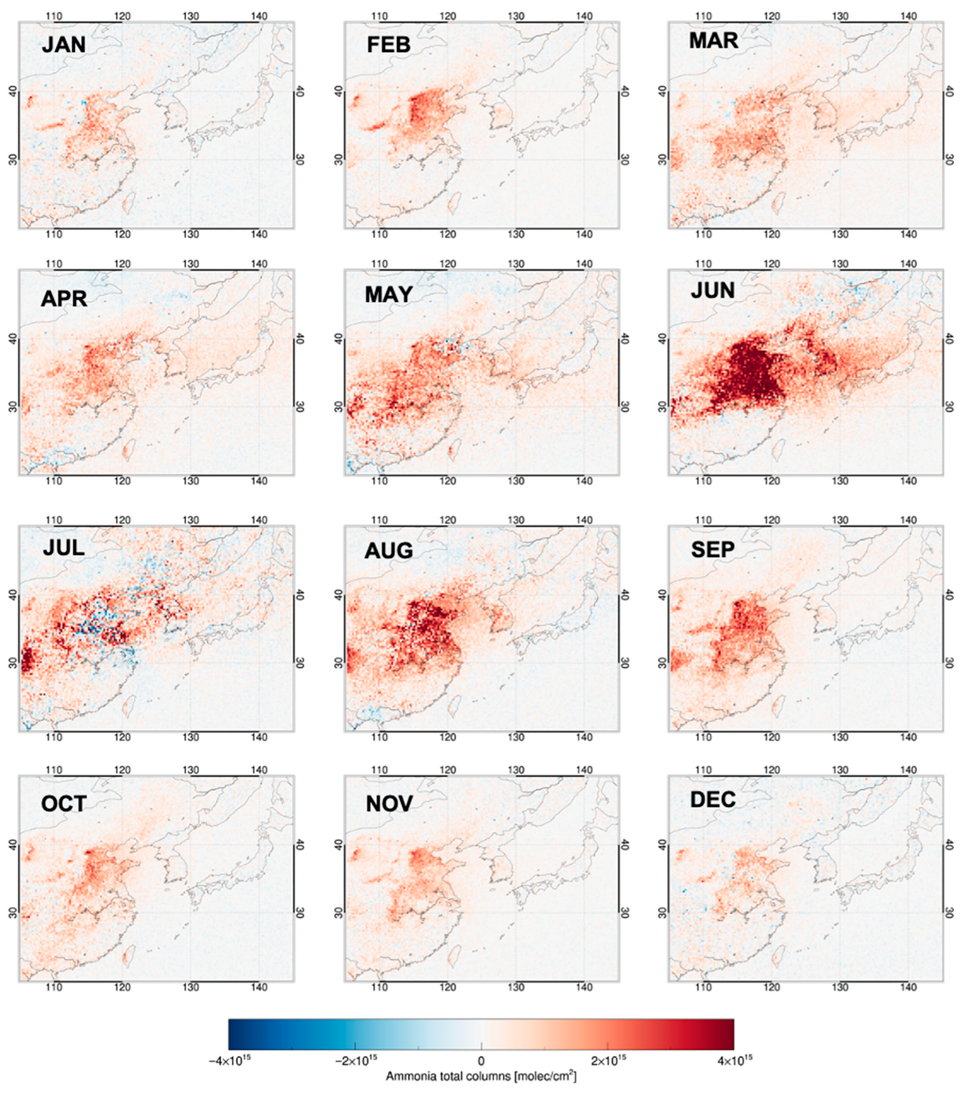
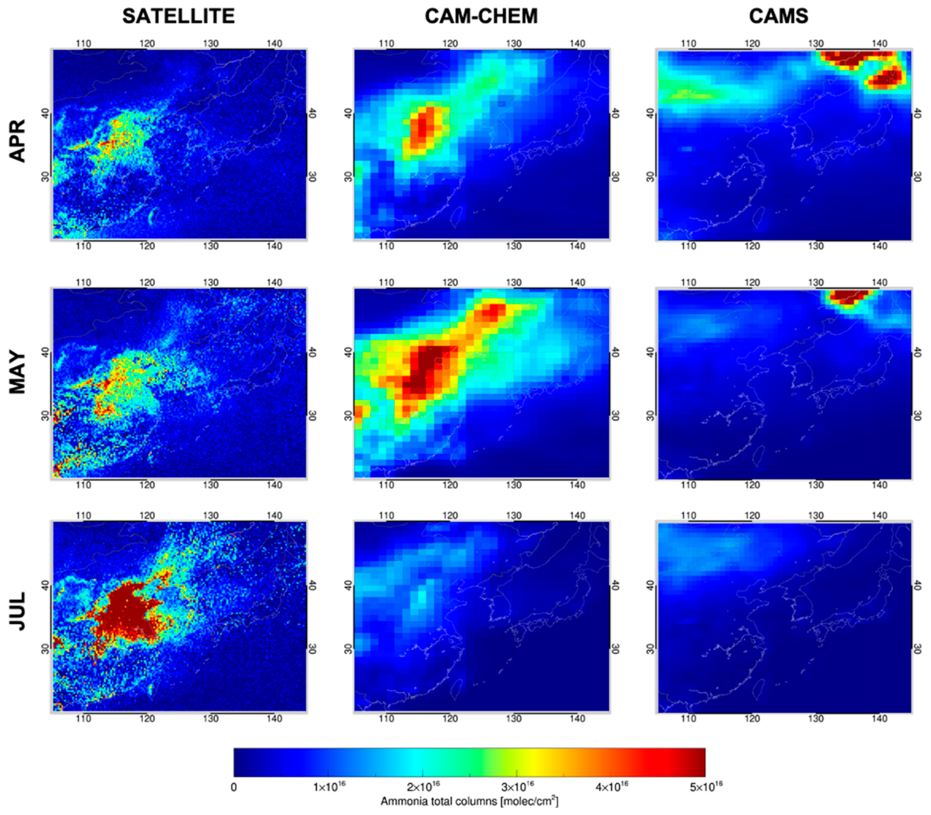
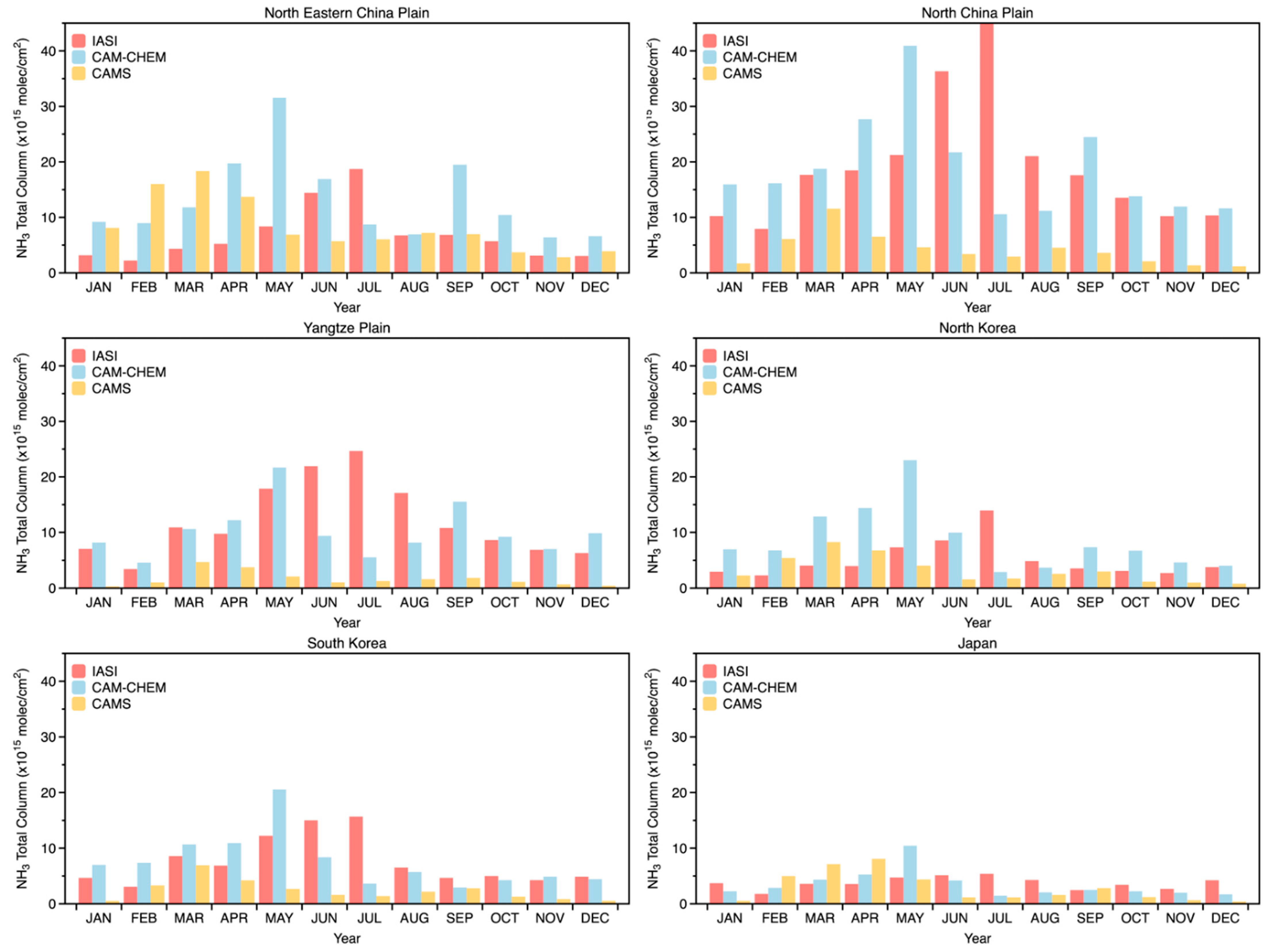
3.2. Comparison Between Satellite Observation and Global Chemical Transport Model

In the previous section, we performed a spatiotemporal analysis using the atmospheric NH₃ concentration actually observation from the IASI. Therefore, we evaluated how well the widely used and readily accessible global CTMs (CAM-Chem and CAMS) simulate the atmospheric NH₃ concentrations in East Asia by comparing them with satellite observations. Figure 7 shows a comparison of monthly NH₃ averages in 2019. Although the grid size of each dataset is different, the seasonal and spatial differences clearly emerged. In terms of spatial distribution, the IASI and CAM-Chem were relatively similar qualitatively, but CAMS showed high concentration in completely different regions. The IASI and CAM-Chem showed high concentrations in the North China Plain and North Eastern China Plain, while CAMS presented high concentrations over Mongolia and Russia. In addition, in terms of seasonal variability, the three datasets exhibited different patterns in East Asia. The maximum NH₃ concentrations occurred in July for the satellite data, in May for CAM-Chem, and in April for CAMS, respectively, as shown in Figure 7 and Figure 8.

In terms of anthropogenic emissions, CAM-Chem utilizes inventories based on EDGAR v4.3.2 and CEDS, which offer a more detailed representation of the seasonal variability associated with region-specific agricultural activities and climate conditions. For instance, the springtime (March–May) peak in fertilizer application is distinctly captured in CAM-Chem. In contrast, CAMS employs the fixed MACCity inventory, resulting in a comparatively weaker representation of seasonal emission patterns. Furthermore, CAM-Chem and CAMS implement different chemical mechanisms—MOZART-T1 and CB05, respectively. MOZART-T1 enables a more sophisticated and accurate simulation of NH₃ reaction pathways and removal processes [47], whereas the relatively simplified CB05 mechanism may underestimate such dynamics. Although CAMS enhances the consistency of modeled atmospheric composition through data assimilation of observational products such as CO, NO₂, O₃, and AOD, NH₃ itself is not assimilated. As a result, in regions with high NH₃ emissions such as agricultural areas in East Asia, CAM-Chem generally shows a more realistic spatial distribution. Overall, CAM-Chem appears to better capture both the spatial and monthly variability of NH₃ concentrations compared to CAMS. However, since CAM-Chem also relies on bottom-up emission inventories [48], discrepancies remain when compared to satellite observations such as the IASI, particularly regarding the timing of maximum concentration periods. These timing discrepancies can partly result from limitations inherent in the bottom-up emission inventories utilized by the CTM, which may not fully capture rapid changes in regional agricultural practices and livestock management. For instance, the actual timing of fertilizer application or manure management in East Asia can vary considerably from year to year due to socioeconomic factors and agricultural policies, but inventories may use fixed or averaged monthly patterns that do not reflect these variations. Additionally, IASI observations may capture real-time changes influenced by weather extremes (e.g., heatwaves or droughts) that significantly alter volatilization rates of NH₃, whereas model inventories often lack such event-specific emission variability. The fact that the spatiotemporal distribution of NH₃ concentration differs across models suggests that there is an urgent need to improve NH₃ emissions when utilizing CTMs.

4. Discussion and Conclusions

In this study, we conducted a comprehensive analysis of atmospheric NH₃ concentrations in East Asia, utilizing long-term satellite observations from 2013 to 2024. We focused on identifying the temporal and spatial distribution of NH₃, and categorized the predominant emission source region. Furthermore, we examined discrepancies between satellite data and chemical transport models.

4.1. Clear Evidence of Seasonal and Spatial Variability

In East Asia, atmospheric NH₃ concentrations show distinct monthly variability, starting to increase in March (spring) to peak in July (summer), then decreasing again to a minimum in winter, particularly marked in areas like the North China Plain and North Eastern China Plain. This seasonal variability observed in our study aligns well with recent satellite-based NH₃ studies [28,49]. Particularly, enhanced agricultural activities such as fertilizer application and livestock waste volatilization during spring and summer months were related as primary contributors to NH₃ emissions. Agricultural lands and livestock operations are identified as significant NH₃ emission sources over East Asia. The spring and summer peaks in NH₃ concentrations correlate with fertilizer application and feedlots, affecting the regional atmospheric conditions. Interestingly, in South Korea, the satellite-derived NH₃ observations show the highest monthly concentrations in June, slightly different from the peak fertilizer-application period (March–May) reported by agricultural emission [50]. This apparent discrepancy can be explained by multiple interacting factors. First, ammonia emitted during intensive spring fertilizer applications likely accumulates in the atmosphere and reaches peak concentrations in June because of its prolonged residence time under warm, dry conditions prior to the onset of the monsoon rains. Second, meteorological conditions in June, characterized by higher temperatures, intense solar radiation, and a stable atmosphere, enhance NH₃ volatilization and limit vertical dispersion, thereby increasing near-surface and column-integrated NH₃ concentrations. This emphasizes the necessity of incorporating seasonal agricultural emission patterns in NH₃ management strategies across East Asia.

4.2. Transition of the Regional Temporal Trends

The temporal variations in NH₃ concentrations across East Asia reveal clear regional contrasts. While the North China Plain exhibited a strong and persistent increase throughout the decade, the North Eastern China Plain experienced stable levels until a rapid rise around 2022, and the Yangtze River Plain showed continuous growth with a slight and brief decline around 2021. These region-specific patterns likely reflect differences in agricultural intensity and emission management effectiveness. In particular, the overall increase in NH₃ concentrations across East Asia can be attributed to multiple interacting factors: (1) increased nitrogen fertilizer use on farmlands to enhance agricultural productivity; (2) expansion of livestock operations, including rising livestock populations and increased livestock density, combined with inadequate manure management practices; and (3) reduced removal rates of NH₃ due to recent emission control policies focused primarily on reducing SO₂ and NO_x emissions, which have inadvertently reduced the atmospheric removal of NH₃ by limiting the formation of ammonium sulfate and nitrate aerosols [16,48,51]. These region-specific patterns likely reflect differences in agricultural intensity and emission management effectiveness [52]. In contrast, South Korea exhibited a continuous and accelerated increase in NH₃ levels, highlighting persistent emissions primarily driven by agricultural practices [53]. These distinct regional differences emphasize the necessity for tailored emission mitigation strategies that consider local agricultural policies and emission control effectiveness to effectively reduce NH₃ concentrations and improve regional air quality. Future emission mitigation strategies should integrate multi-sectoral pollutant management alongside optimized agricultural practices, reflecting specific regional climatic and socioeconomic conditions, to effectively reduce NH₃ concentrations and improve regional air quality across East Asia.

4.3. Spatiotemporal Discrepancies Between Satellite and Chemical Transport Models

In comparing satellite observation with chemical transport models (CAM-Chem and CAMS), substantial discrepancies were identified, particularly in the spatial distribution and seasonal timing of peak NH₃ concentrations. Differences in NH₃ concentrations between the satellite observations (IASI) and chemical transport models (CAM-Chem and CAMS) can be attributed to inherent differences in the observational and modeling platforms. The satellite-derived NH₃ concentrations represent instantaneous snapshots influenced strongly by clear-sky conditions and the thermal contrast within the atmosphere. In contrast, CTMs continuously simulate NH₃ concentrations by incorporating meteorological variability and chemical processes throughout the entire day under all weather conditions. Thus, CTMs may better capture high-concentration events occurring under cloudy or temporally sparse observation conditions, which satellites may miss. Conversely, during optimal observational conditions, IASI measurements can detect high NH₃ concentration peaks more effectively than models, resulting in higher satellite-derived values. Nevertheless, these points primarily address quantitative concentration differences and do not fully explain the substantial spatiotemporal discrepancies demonstrated in analysis.

The pronounced spatiotemporal differences, especially the contrasting seasonal peaks and spatial distribution patterns shown by CAM-Chem and CAMS compared to the IASI, are likely related to limitations in existing emission inventories, chemical mechanisms, and applications. These discrepancies are largely due to inherent limitations of bottom-up emission inventories, which often fail to fully capture rapid and year-to-year variations in agricultural and livestock management practices, as well as episodic meteorological events influencing NH₃ emissions. Recent top-down satellite-based inversion studies revealed that NH₃ emissions in major agricultural areas of East Asia are significantly underestimated by current bottom-up inventories. The seasonal variation in appropriate emission factors can better reflect actual emissions, and by incorporating satellite-derived emission adjustments, discrepancies between observed and modeled NH₃ distributions can be substantially reduced [48,52,54]. Additionally, differences between modeled and observed NH₃ concentrations could also arise due to the rapid conversion of NH₃ to particulate ammonium (NH₄⁺) in acidic atmospheric conditions prevalent in regions such as East Asia, driven by high emissions of acidic precursor gases (e.g., SO₂ and NO_x). This chemical process can significantly decrease modeled NH₃ concentrations compared to satellite observations, contributing further to observed discrepancies [55].

Therefore, the refinement of bottom-up emission inventories through integrating satellite-derived emission estimates, coupled with enhanced chemical reaction mechanisms tailored to regional atmospheric chemistry conditions, is essential for reducing these discrepancies.

Future studies should extend this work by integrating multiple satellite instruments with high-resolution regional chemical transport models to comprehensively characterize NH₃ dynamics over East Asia. Such integrated approaches will allow for improved spatiotemporal analyses and more accurate identification of source-specific contributions to observed NH₃ signals, ultimately supporting targeted and effective regional emission management. Considering the growing significance of NH₃ emissions in East Asia and their substantial impact on regional air quality, our findings highlight the urgent need for strengthened environmental policies and enhanced emission control measures. Establishing accurate and detailed NH₃ emission inventories will be crucial to achieve meaningful improvements in air quality and mitigate future atmospheric pollution.

References

1. Behera, S.N.; Sharma, M.; Aneja, V.P.; Balasubramanian, R. Ammonia in the atmosphere: A review on emission sources, atmospheric chemistry and deposition on terrestrial bodies. Environ. Sci. Pollut. Res. 2013, 20, 8092–8131. [Google Scholar] [CrossRef] [PubMed]
2. Erisman, J.W.; Galloway, J.N.; Seitzinger, S.; Bleeker, A.; Dise, N.B.; Petrescu, A.M.R.; Leach, A.M.; de Vries, W. Consequences of human modification of the global nitrogen cycle. Philos. Trans. R. Soc. B Biol. Sci. 2013, 368, 20130116. [Google Scholar] [CrossRef] [PubMed]
3. Sutton, M.A.; Bleeker, A.; Howard, C.M.; Bekunda, M.; Grizzetti, B.; de Vries, W.; van Grinsven, H.J.M.; Abrol, Y.P.; Adhya, T.K.; Billen, G.; et al. Our Nutrient World: The Challenge to Produce More Food and Energy with Less Pollution; Centre for Ecology and Hydrology: Wallingford, UK, 2013. [Google Scholar]
4. Bouwman, A.F.; Lee, D.S.; Asman, W.A.H.; Dentener, F.J.; Van Der Hoek, K.W.; Olivier, J.G.J. A global high-resolution emission inventory for ammonia. Glob. Biogeochem. Cycles 1997, 11, 561–587. [Google Scholar] [CrossRef]
5. Sutton, M.A.; Reis, S.; Riddick, S.N.; Dragosits, U.; Nemitz, E.; Theobald, M.R.; Tang, Y.S.; Braban, C.F.; Vieno, M.; Dore, A.J.; et al. Towards a climate-dependent paradigm of ammonia emission and deposition. Philos. Trans. R. Soc. Lond. B Biol. Sci. 2013, 368, 20130166. [Google Scholar] [CrossRef] [PubMed]
6. Gu, B.; Zhang, L.; Van Dingenen, R.; Vieno, M.; Van Grinsven, H.J.; Zhang, X.; Zhang, S.; Chen, Y.; Wang, S.; Ren, C.J.S. Abating ammonia is more cost-effective than nitrogen oxides for mitigating PM2.5 air pollution. Science 2021, 374, 758–762. [Google Scholar] [CrossRef] [PubMed]
7. Hauglustaine, D.A.; Balkanski, Y.; Schulz, M.L. A global model simulation of present and future nitrate aerosols and their direct radiative forcing of climate. Atmos. Chem. Phys. 2014, 14, 11031–11063. [Google Scholar] [CrossRef]
8. Phoenix, G.K.; Hicks, W.K.; Cinderby, S.; Kuylenstierna, J.C.I.; Stock, W.D.; Dentener, F.J. Atmospheric nitrogen deposition in world biodiversity hotspots: The need for a greater global perspective in assessing N deposition impacts. Glob. Change Biol. 2006, 12, 470–476. [Google Scholar] [CrossRef]
9. Pye, H.O.T.; Liao, H.; Wu, S.; Mickley, L.J.; Jacob, D.J.; Henze, D.K.; Seinfeld, J.H. Effect of changes in climate and emissions on future sulfate-nitrate-ammonium aerosol levels in the United States. J. Geophys. Res. Atmos. 2009, 114, D01205. [Google Scholar] [CrossRef]
10. Liu, L.; Zhang, X.; Wong, A.Y.H.; Xu, W.; Liu, X.; Li, Y.; Mi, H.; Lu, X.; Zhao, L.; Wang, Z.; et al. Estimating global surface ammonia concentrations inferred from satellite retrievals. Atmos. Chem. Phys. 2019, 19, 12051–12066. [Google Scholar] [CrossRef]
11. Xie, Y.; Wang, W.; Chen, Y.; Qian, Z.; Chen, J.; Tong, J.; Li, L.; Yue, Y.; Chen, K.; Chu, Z.; et al. NH3 Emissions and Lifetime Estimated by Satellite Observations with Differential Evolution Algorithm. Atmosphere 2024, 15, 251. [Google Scholar] [CrossRef]
12. Warner, J.X.; Wei, Z.; Strow, L.L.; Dickerson, R.R.; Nowak, J.B. The global tropospheric ammonia distribution as seen in the 13-year AIRS measurement record. Atmos. Chem. Phys. 2016, 16, 5467–5479. [Google Scholar] [CrossRef]
13. Van Damme, M.; Clarisse, L.; Heald, C.L.; Hurtmans, D.; Ngadi, Y.; Clerbaux, C.; Dolman, A.J.; Erisman, J.W.; Coheur, P.F. Global distributions, time series and error characterization of atmospheric ammonia (NH3) from IASI satellite observations. Atmos. Chem. Phys. 2014, 14, 2905–2922. [Google Scholar] [CrossRef]
14. Van Damme, M.; Wichink Kruit, R.J.; Schaap, M.; Clarisse, L.; Clerbaux, C.; Coheur, P.F. Evaluating 4 years of atmospheric ammonia (NH3) over Europe using IASI satellite observations and LOTOS-EUROS model results. J. Geophys. Res. Atmos. 2014, 119, 9549–9566. [Google Scholar] [CrossRef]
15. Van Damme, M.; Clarisse, L.; Dammers, E.; Liu, X.; Nowak, J.B.; Clerbaux, C.; Flechard, C.R.; Galy-Lacaux, C.; Xu, W.; Neuman, J.A.; et al. Towards validation of ammonia (NH3) measurements from the IASI satellite. Atmos. Meas. Tech. 2015, 8, 1575–1591. [Google Scholar] [CrossRef]
16. Warner, J.X.; Dickerson, R.R.; Wei, Z.; Strow, L.L.; Wang, Y.; Liang, Q. Increased atmospheric ammonia over the world’s major agricultural areas detected from space. Geophys. Res. Lett. 2017, 44, 2875–2884. [Google Scholar] [CrossRef] [PubMed]
17. Nair, A.A.; Yu, F.; Luo, G. Spatioseasonal variations of atmospheric ammonia concentrations over the United States: Comprehensive model-observation comparison. J. Geophys. Res. Atmos. 2019, 124, 6571–6582. [Google Scholar] [CrossRef]
18. Van Damme, M.; Clarisse, L.; Whitburn, S.; Hadji-Lazaro, J.; Hurtmans, D.; Clerbaux, C.; Coheur, P.F. Industrial and agricultural ammonia point sources exposed. Nature 2018, 564, 99–103. [Google Scholar] [CrossRef] [PubMed]
19. Schiferl, L.D.; Heald, C.L.; Damme, M.V.; Clarisse, L.; Clerbaux, C.; Coheur, P.-F.; Nowak, J.B.; Andrew Neuman, J.; Herndon, S.C.; Roscioli, J.R.; et al. Interannual variability of ammonia concentrations over the United States: Sources and implications. Atmos. Chem. Phys. 2016, 16, 12305–12328. [Google Scholar] [CrossRef]
20. Zhang, X.; Tran, D.A.; Van Nguyen, D.; Sato, H.; Eto, Y.; Aikawa, M. Concentration characteristics and wavelet analysis of ambient NH3 in Kitakyushu, Japan over the period of 2018–2022. Water Air Soil Pollut. 2025, 236, 60. [Google Scholar] [CrossRef]
21. Zhou, M.; Deng, Z.; Robert, C.; Zhang, X.; Zhang, L.; Wang, Y.; Qi, C.; Wang, P.; De Mazière, M. The first global map of atmospheric ammonia (NH3) as observed by the HIRAS/FY-3D satellite. Adv. Atmos. Sci. 2024, 41, 379–390. [Google Scholar] [CrossRef]
22. Ma, J.; Shi, H.; Zhu, Y.; Li, R.; Wang, S.; Lu, N.; Yao, Y.; Bian, Z.; Huang, K. The evolution of global surface ammonia concentrations during 2001–2019: Magnitudes, patterns, and drivers. Environ. Sci. Technol. 2025, 59, 5066–5079. [Google Scholar] [CrossRef] [PubMed]
23. Silveira, B.B.; Fourrié, N.; Guidard, V.; Chambon, P.; Mahfouf, J.-F.; Brousseau, P.; Moll, P.; August, T.; Hultberg, T. Preliminary Assessment of MetOp-Based Temperature and Humidity Statistical Retrievals within the 3D-Var AROME-France Prediction System. Mon. Wea. Rev. 2022, 150, 733–752. [Google Scholar] [CrossRef]
24. Della Fera, S.; Fabiano, F.; Raspollini, P.; Ridolfi, M.; Cortesi, U.; Barbara, F.; von Hardenberg, J. On the use of Infrared Atmospheric Sounding Interferometer (IASI) spectrally resolved radiances to test the EC-Earth climate model (v3.3.3) in clear-sky conditions. Geosci. Model Dev. 2023, 16, 1379–1394. [Google Scholar] [CrossRef]
25. Clarisse, L.; Franco, B.; Van Damme, M.; Di Gioacchino, T.; Hadji-Lazaro, J.; Whitburn, S.; Noppen, L.; Hurtmans, D.; Clerbaux, C.; Coheur, P. The IASI NH3 version 4 product: Averaging kernels and improved consistency. Atmos. Meas. Tech. 2023, 16, 5009–5028. [Google Scholar] [CrossRef]
26. Clarisse, L.; Shephard, M.W.; Dentener, F.; Hurtmans, D.; Cady-Pereira, K.; Karagulian, F. Satellite monitoring of ammonia: A case study of the San Joaquin Valley. J. Geophys. Res. 2010, 115, D13302. [Google Scholar] [CrossRef]
27. Wang, R.; Guo, X.; Pan, D.; Kelly, J.T.; Bash, J.O.; Sun, K. Monthly patterns of ammonia over the contiguous United States at 2-km resolution. Geophys. Res. Lett. 2021, 48, e2020GL090579. [Google Scholar] [CrossRef] [PubMed]
28. Luo, Z.; Zhang, Y.; Chen, W.; Van Damme, M.; Coheur, P.F.; Clarisse, L. Estimating global ammonia (NH3) emissions based on IASI observations from 2008 to 2018. Atmos. Chem. Phys. 2022, 22, 10375–10388. [Google Scholar] [CrossRef]
29. Lamarque, J.-F.; Emmons, L.K.; Hess, P.G.; Kinnison, D.E.; Tilmes, S.; Vitt, F.; Heald, C.L.; Holland, E.A.; Lauritzen, P.H.; Neu, J.; et al. CAM-chem: Description and evaluation of interactive atmospheric chemistry in the Community Earth System Model. Geosci. Model Dev. 2012, 5, 369–411. [Google Scholar] [CrossRef]
30. Buchholz, R.R.; Emmons, L.K.; Tilmes, S.; The CESM2 Development Team. CESM2.1/CAM-chem Instantaneous Output for Boundary Conditions. UCAR/NCAR—Atmospheric Chemistry Observations and Modeling Laboratory 2019, Subset Used Lat: 10 to 80, Lon: 60 to 240, January 2013–December 2021. Available online: https://wiki.ucar.edu/spaces/camchem/pages/372834733/CESM2.1+CAM-chem+as+Boundary+Conditions (accessed on 21 March 2025).
31. Emmons, L.K.; Schwantes, R.H.; Orlando, J.J.; Tyndall, G.; Kinnison, D.; Lamarque, J.-F.; Marsh, D.; Mills, M.J.; Tilmes, S.; Bardeen, C.; et al. The chemistry mechanism in the community earth system model version 2 (CESM2). J. Adv. Model. Earth Syst. 2020, 12, e2019MS001882. [Google Scholar] [CrossRef]
32. Liu, X.; Ma, P.-L.; Wang, H.; Tilmes, S.; Singh, B.; Easter, R.C.; Ghan, S.J.; Rasch, P.J. Description and evaluation of a new four-mode version of the Modal Aerosol Module (MAM4) within version 5.3 of the Community Atmosphere Model. Geosci. Model Dev. 2016, 9, 505–522. [Google Scholar] [CrossRef]
33. Tilmes, S.; Hodzic, A.; Emmons, L.K.; Mills, M.J.; Gettelman, A.; Kinnison, D.E.; Park, M.; Lamarque, J.-F.; Vitt, F.; Shrivastava, M.; et al. Climate forcing and trends of organic aerosols in the Community Earth System Model (CESM2). J. Adv. Model. Earth Syst. 2019, 11, 4323–4351. [Google Scholar] [CrossRef]
34. Crippa, M.; Guizzardi, D.; Muntean, M.; Schaaf, E.; Dentener, F.; van Aardenne, J.A.; Monni, S.; Doering, U.; Olivier, J.G.J.; Pagliari, V.; et al. Gridded emissions of air pollutants for the period 1970–2012 within EDGAR v4.3.2. Earth Syst. Sci. Data 2018, 10, 1987–2013. [Google Scholar] [CrossRef]
35. Hoesly, R.M.; Smith, S.J.; Feng, L.; Klimont, Z.; Janssens-Maenhout, G.; Pitkanen, T.; Seibert, J.J.; Vu, L.; Andres, R.J.; Bolt, R.M.; et al. Historical (1750–2014) anthropogenic emissions of reactive gases and aerosols from the Community Emissions Data System (CEDS). Geosci. Model Dev. 2018, 11, 369–408. [Google Scholar] [CrossRef]
36. Guenther, A.B.; Karl, T.; Harley, P.; Wiedinmyer, C.; Palmer, P.I.; Geron, C. Estimates of global terrestrial isoprene emissions using MEGAN (Model of Emissions of Gases and Aerosols from Nature). Atmos. Chem. Phys. 2006, 6, 3181–3210. [Google Scholar] [CrossRef]
37. Guenther, A.B.; Jiang, X.; Heald, C.L.; Sakulyanontvittaya, T.; Duhl, T.; Emmons, L.K.; Wang, X. The Model of Emissions of Gases and Aerosols from Nature version 2.1(MEGAN2.1): An extended and updated framework for modeling biogenic emissions. Geosci. Model Dev. 2012, 5, 1471–1492. [Google Scholar] [CrossRef]
38. Wiedinmyer, C.; Akagi, S.K.; Yokelson, R.J.; Emmons, L.K.; Al-Saadi, J.A.; Orlando, J.J.; Soja, A.J. The Fire INventory from NCAR (FINN): A high resolution global model to estimate the emissions from open burning. Geosci. Model Dev. 2011, 4, 625–641. [Google Scholar] [CrossRef]
39. Inness, A.; Ades, M.; Agustí-Panareda, A.; Barré, J.; Benedictow, A.; Blechschmidt, A.-M.; Dominguez, J.J.; Engelen, R.; Eskes, H.; Flemming, J.; et al. The CAMS reanalysis of atmospheric composition. Atmos. Chem. Phys. 2019, 19, 3515–3556. [Google Scholar] [CrossRef]
40. Yarwood, G.; Rao, S.; Yocke, M.; Whitten, G. Updates to the Carbon Bond Chemical Mechanism: CB05. Final Report to the US EPA; EPA Report Number: RT-0400675; United States Environmental Protection Agency: Washington, DC, USA, 2005.
41. Huijnen, V.; Williams, J.; van Weele, M.; van Noije, T.; Krol, M.; Dentener, F.; Segers, A.; Houweling, S.; Peters, W.; de Laat, J.; et al. The global chemistry transport model TM5: Description and evaluation of the tropospheric chemistry version 3.0. Geosci. Model Dev. 2010, 3, 445–473. [Google Scholar] [CrossRef]
42. Granier, C.; Bessagnet, B.; Bond, T.; D’Angiola, A.; Denier van der Gon, H.; Frost, G.J.; Heil, A.; Kaiser, J.W.; Kinne, S.; Klimont, Z.; et al. Evolution of anthropogenic and biomass burning emissions of air pollutants at global and regional scales during the 1980–2010 period. Clim. Change 2011, 109, 163–190. [Google Scholar] [CrossRef]
43. Sindelarova, K.; Granier, C.; Bouarar, I.; Guenther, A.; Tilmes, S.; Stavrakou, T.; Müller, J.-F.; Kuhn, U.; Stefani, P.; Knorr, W. Global data set of biogenic VOC emissions calculated by the MEGAN model over the last 30 year. Atmos. Chem. Phys. 2014, 14, 9317–9341. [Google Scholar] [CrossRef]
44. Kaiser, J.W.; Heil, A.; Andreae, M.O.; Benedetti, A.; Chubarova, N.; Jones, L.; Morcrette, J.-J.; Razinger, M.; Schultz, M.G.; Suttie, M.; et al. Biomass burning emissions estimated with a global fire assimilation system based on observed fire radiative power. Biogeosciences 2012, 9, 527–554. [Google Scholar] [CrossRef]
45. Gilbert, M.; Nicolas, G.; Cinardi, G.; Boeckel, T.P.V.; Vanwambeke, S.O.; Wint, G.R.W.; Robinson, T.P. Global distribution data for cattle, buffaloes, horses, sheep, goats, pigs, chickens and ducks in 2010. Sci. Data 2018, 5, 180227. [Google Scholar] [CrossRef] [PubMed]
46. Otte, J.; Pica-Ciamarra, U.; Morzaria, S. A comparative overview of the livestock-environment interactions in Asia and Sub-Saharan Africa. Front. Vet. Sci. 2019, 6, 37. [Google Scholar] [CrossRef] [PubMed]
47. Zaveri, R.A.; Easter, R.C.; Singh, B.; Wang, H.; Lu, Z.; Tilmes, S.; Emmons, L.K.; Vitt, F.; Zhang, R.; Liu, X.; et al. Development and evaluation of chemistry-aerosol-climate model CAM5-Chem-MAM7-MOSAIC: Global atmospheric distribution and radiative effects of nitrate aerosol. J. Adv. Model. Earth Syst. 2021, 13, e2020MS002346. [Google Scholar] [CrossRef] [PubMed]
48. Zhang, L.; Chen, Y.; Zhao, Y.; Henze, D.K.; Zhu, L.; Song, Y.; Paulot, F.; Liu, X.; Pan, Y.; Lin, Y.; et al. Agricultural ammonia emissions in China: Reconciling bottom-up and top-down estimates. Atmos. Chem. Phys. 2018, 18, 339–355. [Google Scholar] [CrossRef]
49. Van Damme, M.; Clarisse, L.; Franco, B.; Sutton, M.A.; Erisman, J.W.; Kruit, R.W.; Van Zanten, M.; Whitburn, S.; Hadji-Lazaro, J.; Hurtmans, D. Global, Regional and National Trends of Atmospheric Ammonia Derived from a Decadal (2008–2018) Satellite Record. Environ. Res. Lett. 2021, 16, 055017. [Google Scholar] [CrossRef]
50. Park, J.; Lee, S.-Y.; Hong, S.-W.; Na, R.; Oh, Y. Spatio-temporal change analysis of ammonia emission estimation for fertilizer application cropland using high-resolution farmland data. J. Korean Soc. Rural. Plan. 2021, 27, 33–41. [Google Scholar]
51. Xu, R.T.; Pan, S.F.; Chen, J.; Chen, G.S.; Yang, J.; Dangal, S.R.S.; Shepard, J.P.; Tian, H.Q. Half-century ammonia emissions from agricultural systems in southern Asia: Magnitude, spatiotemporal patterns, and implications for human health. Geohealth 2018, 2, 40–53. [Google Scholar] [CrossRef] [PubMed]
52. Chen, J.; Cheng, M.; Krol, M.; de Vries, W.; Zhu, Q.; Liu, X.; Zhang, F.; Xu, W. Trends in anthropogenic ammonia emissions in China since 1980: A review of approaches and estimations. Front. Environ. Sci. 2023, 11, 1133753. [Google Scholar] [CrossRef]
53. Kuttippurath, J.; Patel, V.K.; Kashyap, R.; Singh, A.; Clerbaux, C. Anomalous increase in global atmospheric ammonia during COVID-19 lockdown: Need policies to curb agricultural emissions. J. Clean. Prod. 2023, 434, 140424. [Google Scholar] [CrossRef]
54. Momeni, M.; Choi, Y.; Yeganeh, A.K.; Pouyaei, A.; Jung, J.; Park, J.; Shephard, M.W.; Dammers, E.; Cady-Pereira, K.E. Constraining East Asia ammonia emissions through satellite observations and iterative Finite Difference Mass Balance (iFDMB) and investigating its impact on inorganic fine particulate matter. Environ. Int. 2024, 184, 108473. [Google Scholar] [CrossRef] [PubMed]
55. Pawar, P.V.; Ghude, S.D.; Jena, C.; Móring, A.; Sutton, M.A.; Kulkarni, S.; Lal, D.M.; Surendran, D.; Van Damme, M.; Clarisse, L. Analysis of Atmospheric Ammonia over South and East Asia Based on the MOZART-4 Model and Its Comparison with Satellite and Surface Observations. Atmos. Chem. Phys. 2021, 21, 6389–6409. [Google Scholar] [CrossRef]
Figure 1. The domain of the East Asia region and region of interests. The spatial distribution of background is the terrain height from Earth TOPOgraphy (ETOPO)-2 dataset.
Remotesensing 17 02587 g001
Figure 2. Spatial distribution of monthly averaged NH3 atmospheric concentrations derived from IASI/MetOp-B for the period of 2013–2024. NH3 concentration data were selected based on pre- and post-retrieval quality flags under cloud-free conditions (cloud cover < 10%) and oversampled onto a 0.25° × 0.25° grid. The areas exceeding 5 × 10¹⁷ molecules cm−2 were indicated with the same color to facilitate easier identification of seasonal variation in the spatial distribution.
Remotesensing 17 02587 g002
Figure 3. Monthly variation in average NH3 concentrations from 2013 to 2024 in representative large cities (left) and farmlands (right).
Remotesensing 17 02587 g003
Figure 4. Spatial distribution of linear trends in NH3 atmospheric concentrations derived from IASI/MetOp-B for the period of 2013–2024. The linear trends were calculated using the monthly averaged data oversampled onto a 0.25° × 0.25° grid.
Remotesensing 17 02587 g004
Figure 5. The time series of decomposition results: (left) observations, (middle) trends, and (right) seasonality for each region.
Remotesensing 17 02587 g005
Figure 6. Regions classified by NH3 concentration and monthly variability from K-means method. And normalized monthly variation for each category.
Remotesensing 17 02587 g006
Figure 7. Spatial distributions of monthly mean atmospheric NH3 total columns over East Asia in 2019 derived from IASI satellite observations, CAM-Chem model simulations, and CAMS reanalysis data. Panels correspond to April, May, and July, months when maximum NH3 concentrations occur for CAMS (April), CAM-Chem (May), and IASI (July), respectively.
Remotesensing 17 02587 g007
Figure 8. Comparison of monthly averages of atmospheric NH3 concentration of each region for IASI, CAM-Chem, and CAMS.
Remotesensing 17 02587 g008
Disclaimer/Publisher’s Note: The statements, opinions and data contained in all publications are solely those of the individual author(s) and contributor(s) and not of MDPI and/or the editor(s). MDPI and/or the editor(s) disclaim responsibility for any injury to people or property resulting from any ideas, methods, instructions or products referred to in the content.