
A Novel Hybrid Fuzzy Comprehensive Evaluation and Machine Learning Framework for Solar PV Suitability Mapping in China


Abstract
1. Introduction
- (1)
- Proposes a comprehensive suitability evaluation criteria system that integrate meteorological, topographic, and economic cost–benefit criteria.
- (2)
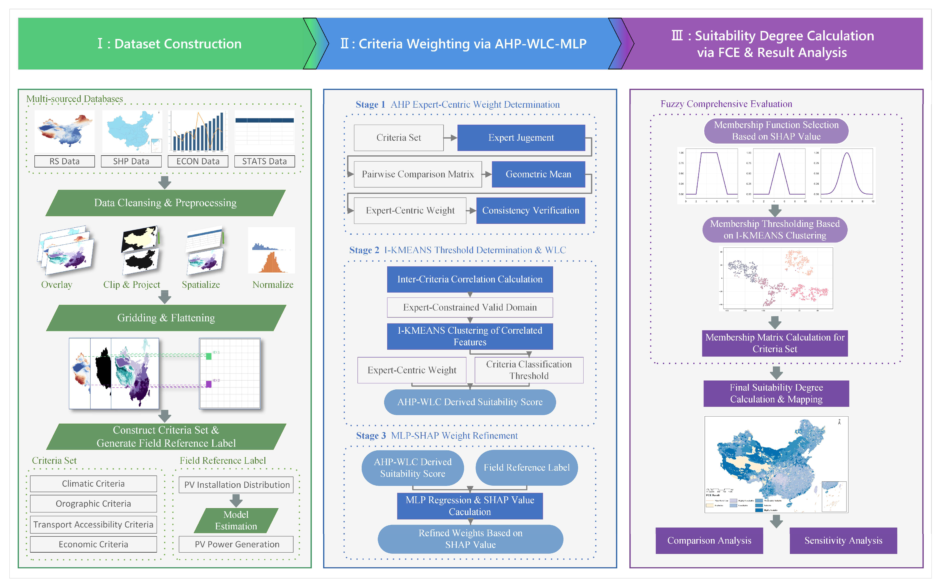
- Proposes a novel dual-stage AHP–WLC–MLP framework that integrates the I-KMEANS algorithm. This approach aims to overcome the traditional WLC method’s reliance on subjective experience in threshold determination.
- (3)
- Introduces the Fuzzy Comprehensive Evaluation (FCE) method to mitigate semantic ambiguity arising from rigid classification schemes by quantifying fuzzy membership relationships across suitability levels. Additionally, it proposes the FAI to measure fuzzy association intensity, thereby providing an improved approach for sensitivity analysis.
2. Materials and Methods
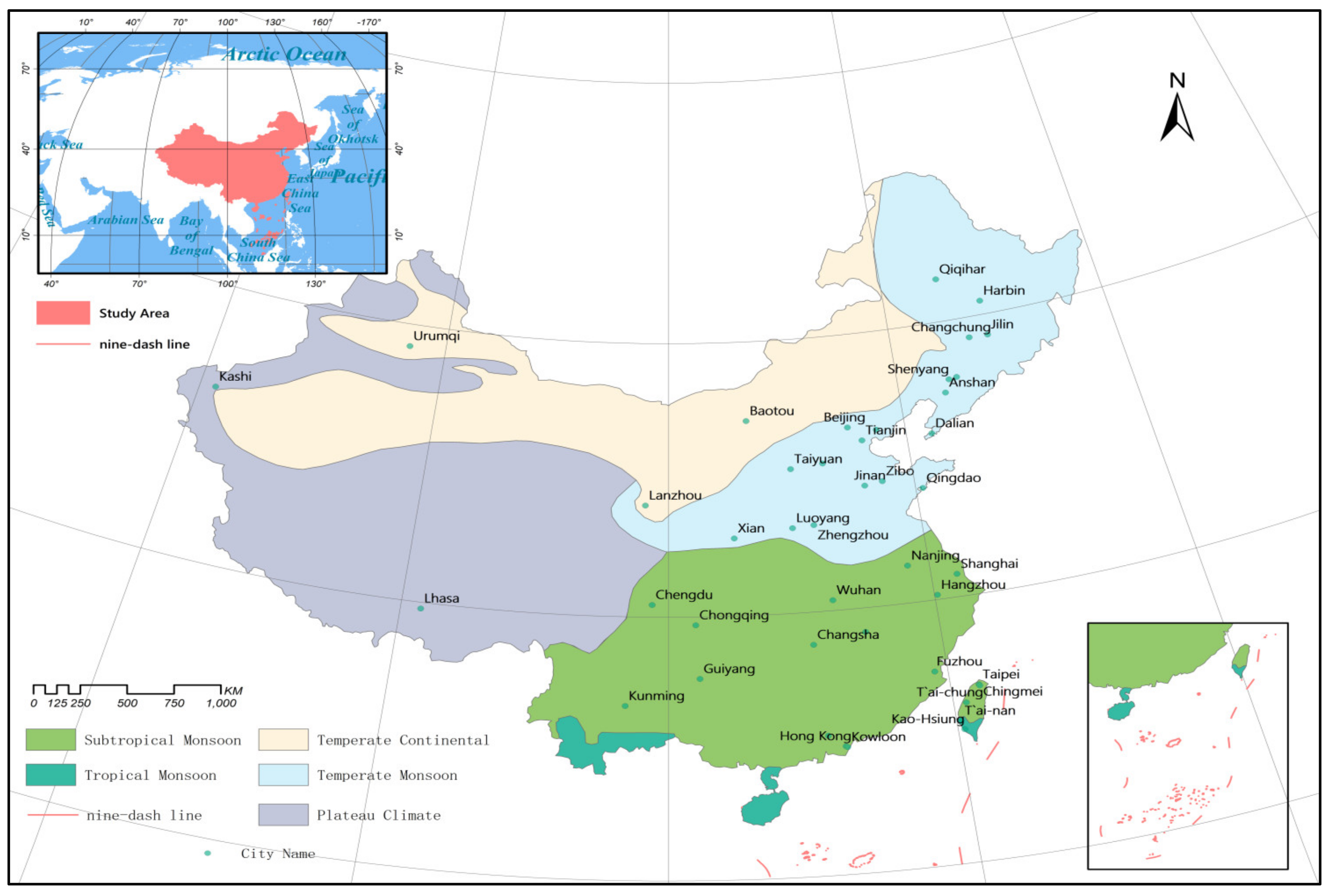
2.1. Study Area
2.2. Data Source
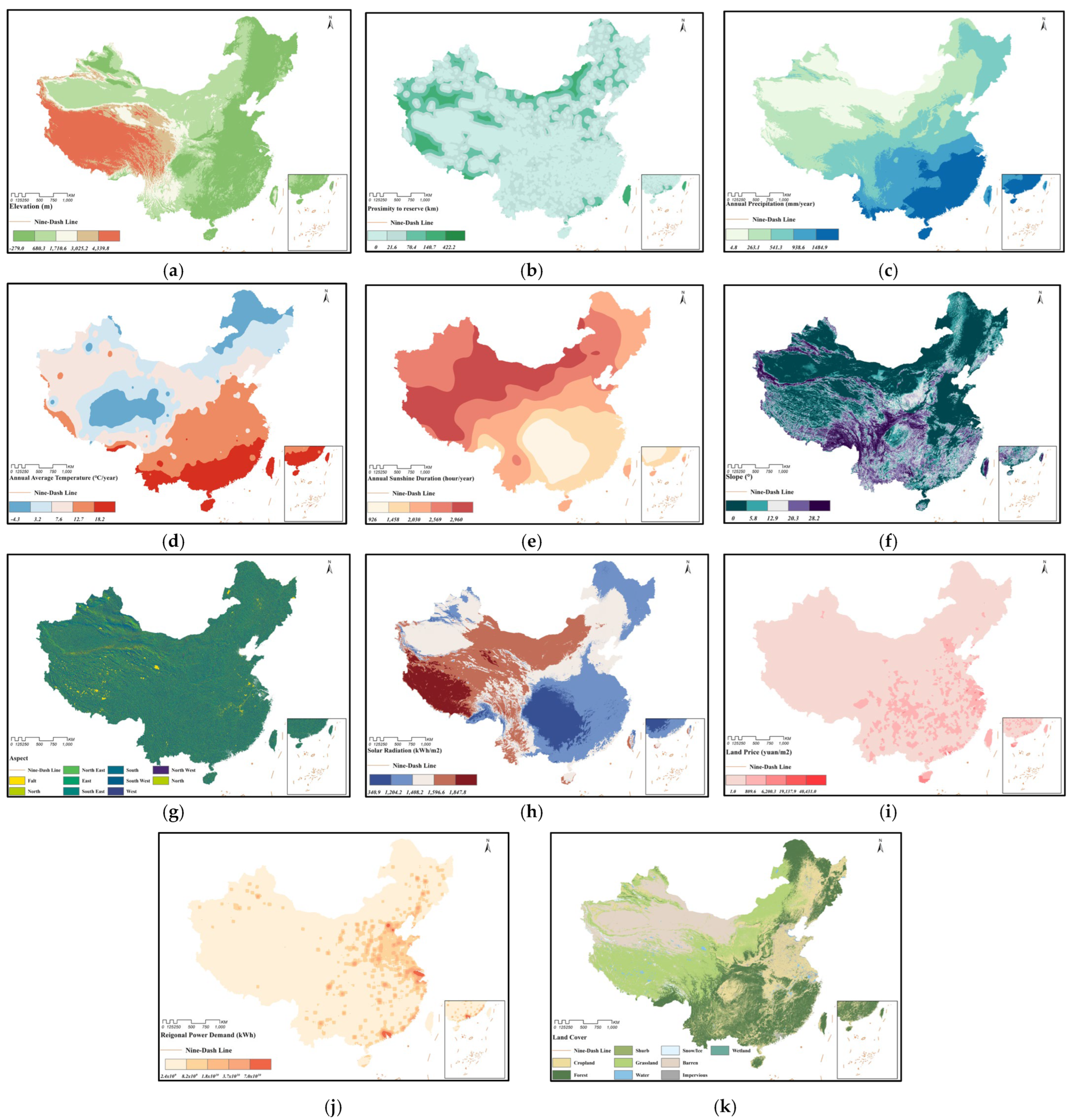
2.2.1. Data
- (1)
- Criteria Data
- (2)
- Non-Criteria Data
2.2.2. Data Preprocessing
2.3. Decision Set Selection
2.4. Weight Determination
2.4.1. AHP–WLC Label Generation
- (1)
- Expert-Driven Weight Determination Via AHP
- (2)
- Determination of WLC Thresholds via I-KMEANS
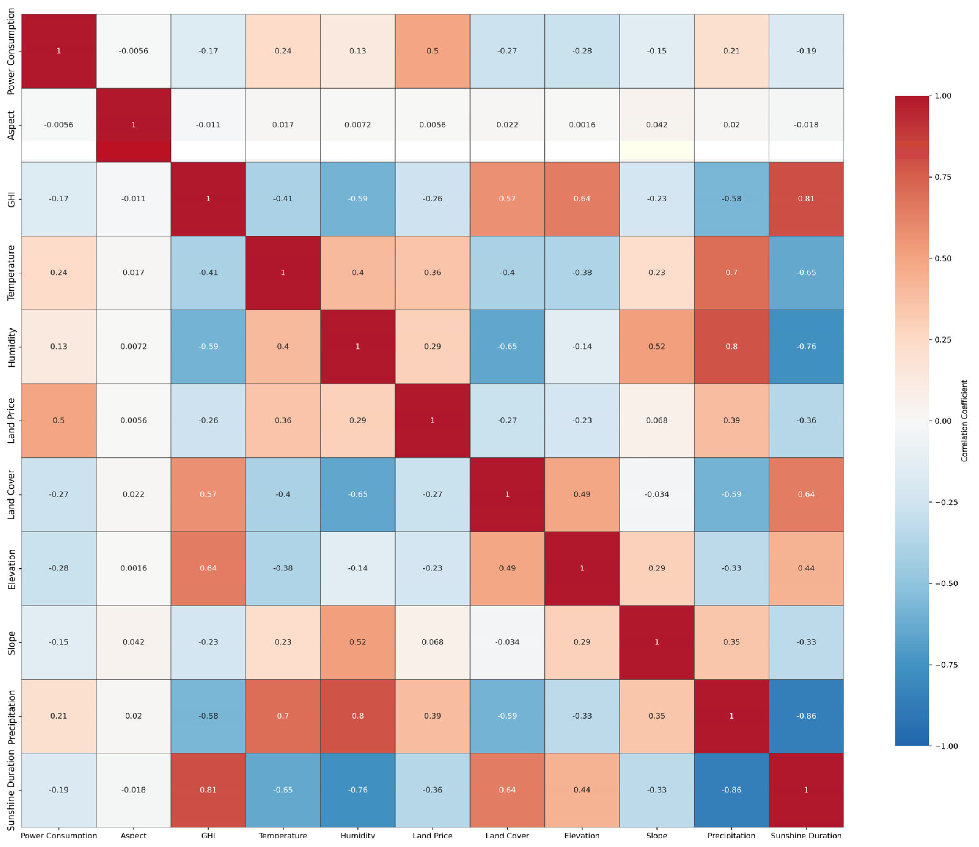
- Computation of Inter-Factor Correlations
- Expert-Driven Threshold Determination
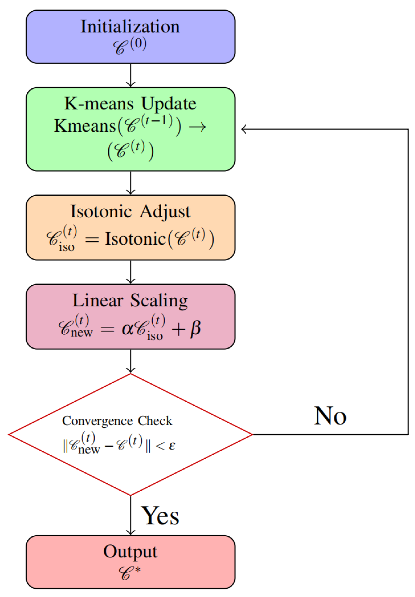
- I-KMEANS
- (i)
- Isotonic regression: Isotonic regression modifies each column of the unconstrained cluster centroids individually to satisfy the specified monotonicity constraints. For individual columns, the adjustment objective can be expressed as:In this study, the PAV (Pool Adjacent Violators) algorithm was utilized to perform isotonic regression. Initially, each observation is treated as an independent block, and a monotonic sequence is constructed by iteratively merging adjacent blocks that violate the monotonicity constraint using weighted averaging. The process can be formally expressed asIn the equation, Bj denotes the jth block, wi represents the weight of the ith sample, yi is the value of the ith sample, µj refers to the mean of block Bj, and µnew indicates the mean of the newly merged block. One iteration of the PAV algorithm is completed by assigning µnew to all values in the merged violating blocks. The process ends when all blocks meet the required monotonicity.
- (ii)
- Result perturbation: Equal group sizes across successive iterations frequently result in identical values along the same dimension. A perturbation strategy is applied to identical entries in the isotonic regression output, following this rule:
- (iii)
- Result scaling: Final results are derived through column-wise scaling of the perturbed centroids.Parameters a and b in the scaling formula are optimized on a per-column basis using the Sequential Least-Squares Quadratic Programming (SLSQP) algorithm, with the objective of minimizing the deviation between the scaled and original values while simultaneously maximizing the variance within each column. Predefined weighting coefficients are introduced to balance the dual objectives, thereby ensuring that the scaled data retains key structural characteristics of the original data while promoting more uniform distributions across columns.where λ1, λ2 are hyperparameters controlling the variance and distribution constraint weights, respectively. Vmin is the minimum variance threshold, and ∆min is the minimum spacing requirement (both are hyperparameters).
- (3)
- Result Computation Via WLC
2.4.2. Training Sample Generation
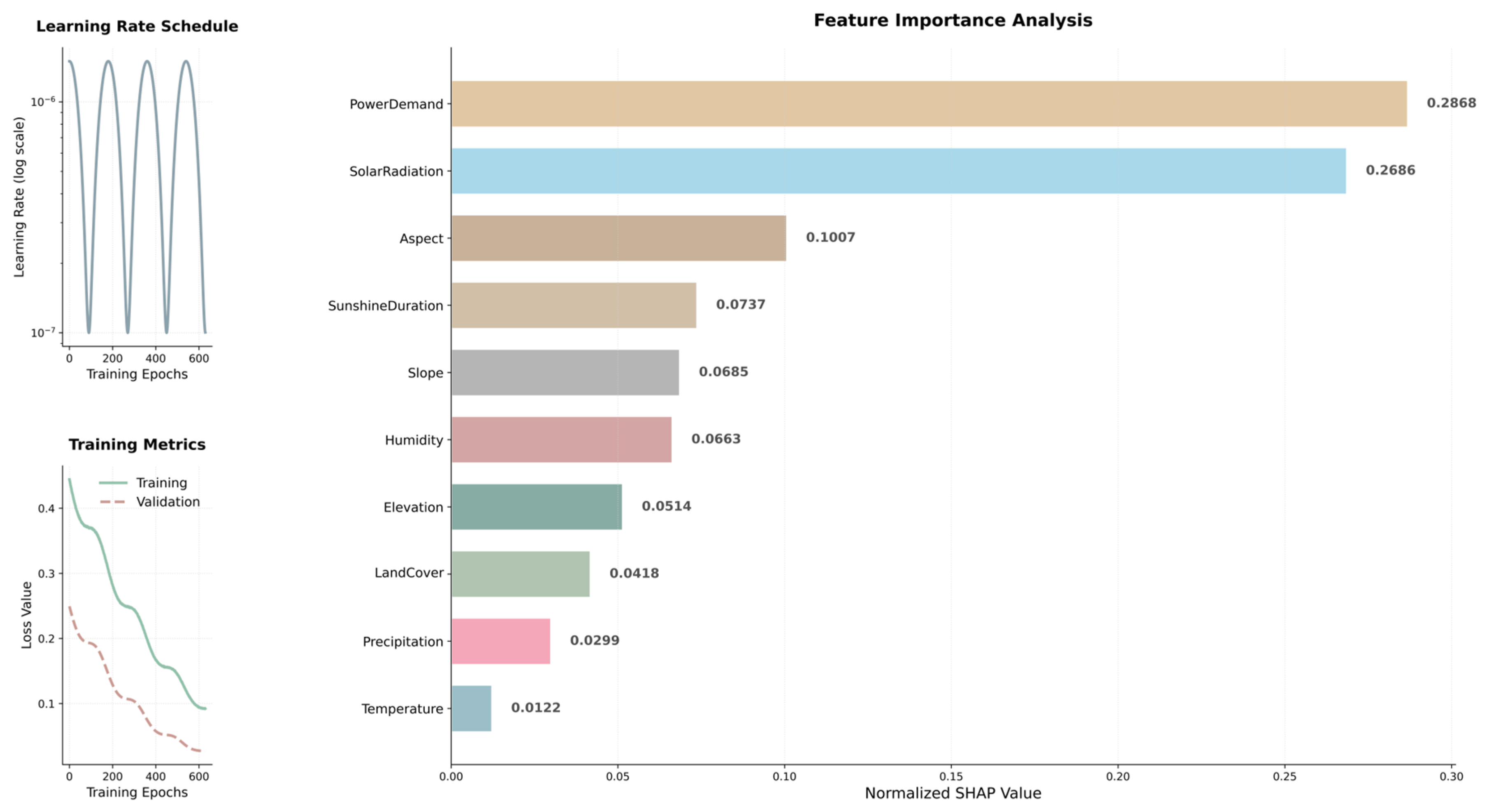
2.4.3. Refined Weight Determination Via MLP
- Input vector: x ∈ Rd (d-dimensional features)
- Hidden layer: W(1) ∈ Rh×d (weight matrix), b(1) ∈ Rh (bias vector)
- Output layer: W(2) ∈ Ro×h (weight matrix), b(2) ∈ Ro (bias vector)
- g(·): Hidden layer Activation (E.G., Relu: g(z) = max(0, z))
2.5. Suitability Evaluation Result Computation
2.5.1. Fuzzy Correlation Matrix Computation
- (1)
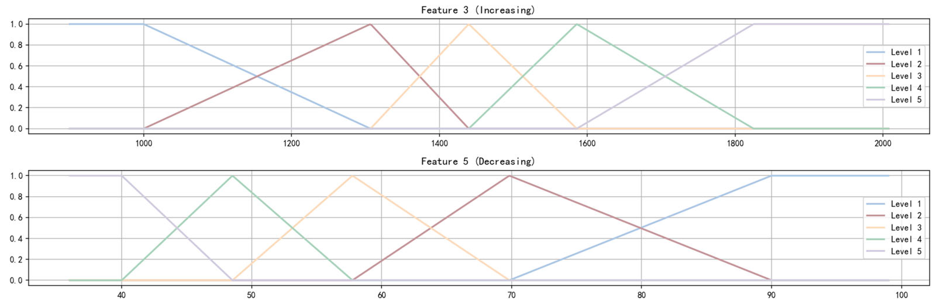
- Combination and Selection of Membership Functions
Single-Factor Fuzzy Correlation Vector Computation
- (2)
- Membership Matrix Computation
2.5.2. Weighted Result Computation
2.5.3. Result Computation
3. Result
3.1. Threshold Classification Results Based on I-KMEANS
3.2. MLP-Based Weight Determination
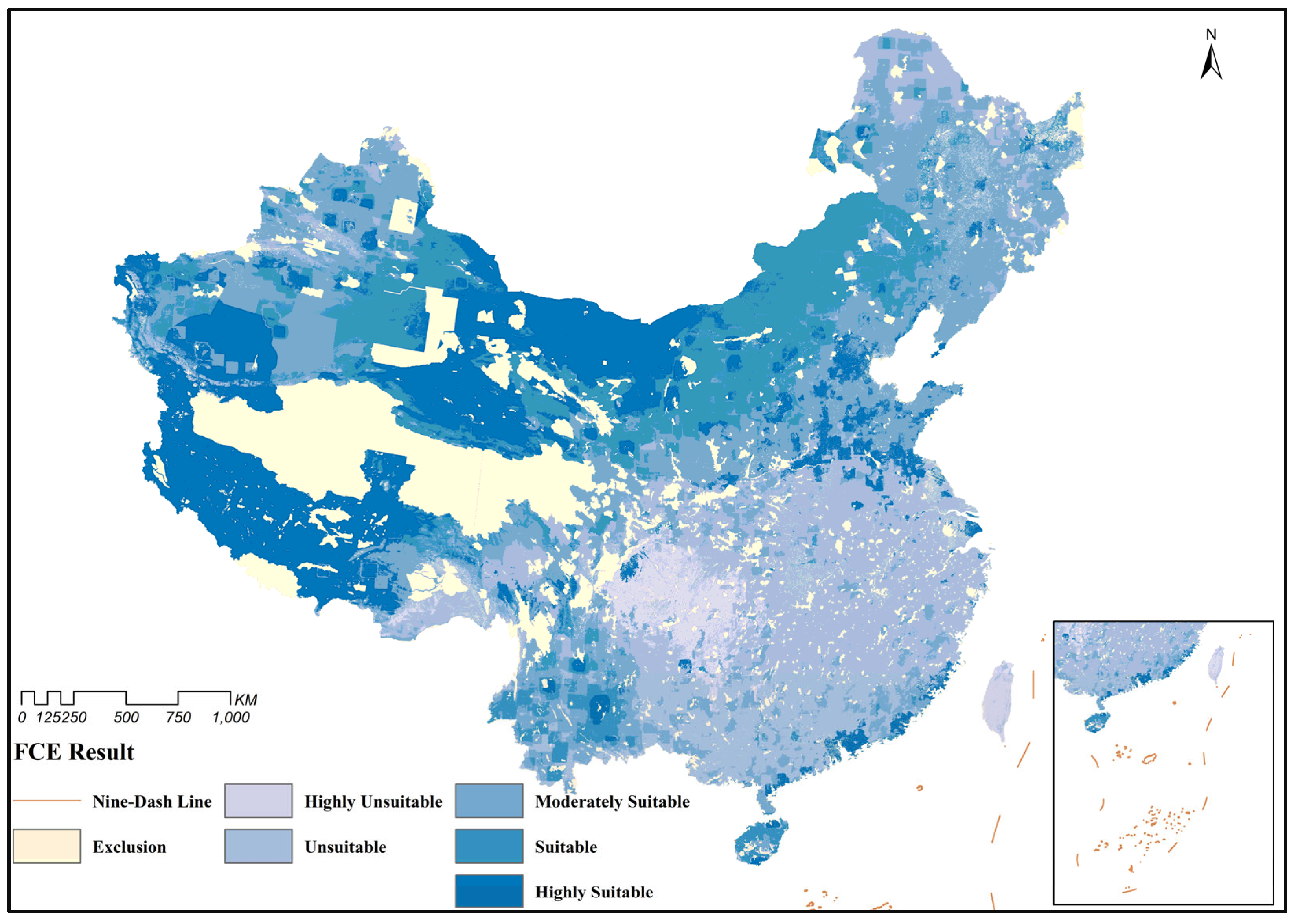
3.3. Suitability Assessment Results
3.4. Analysis of Result
3.4.1. Analysis of National Suitability Evaluation Results
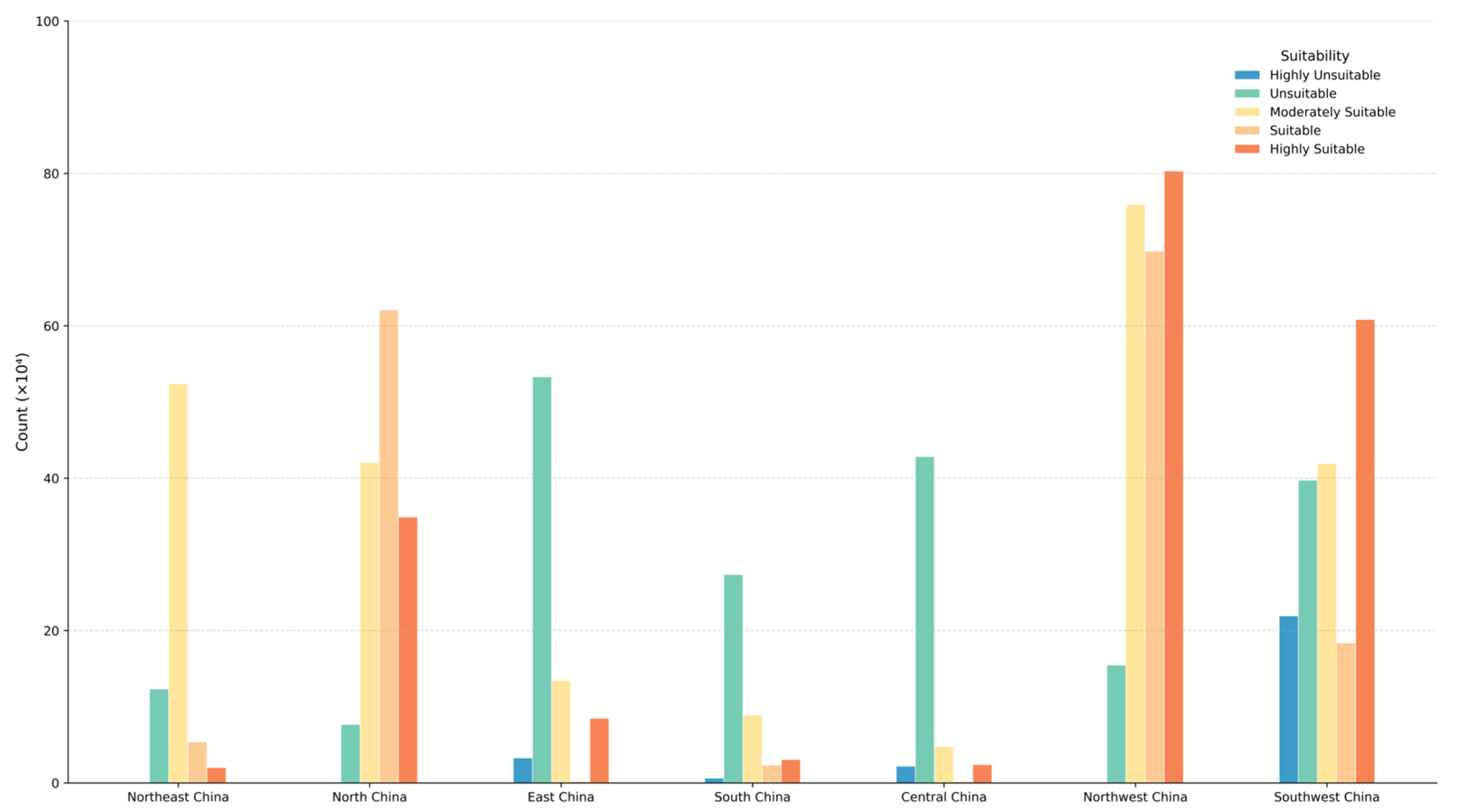
3.4.2. Analysis of Regional Suitability Evaluation Results
3.5. Threshold Determination Algorithm Experiment
3.5.1. Comparative Experiments
3.5.2. Ablation Study
3.6. Comparison of Weight Determination Methods
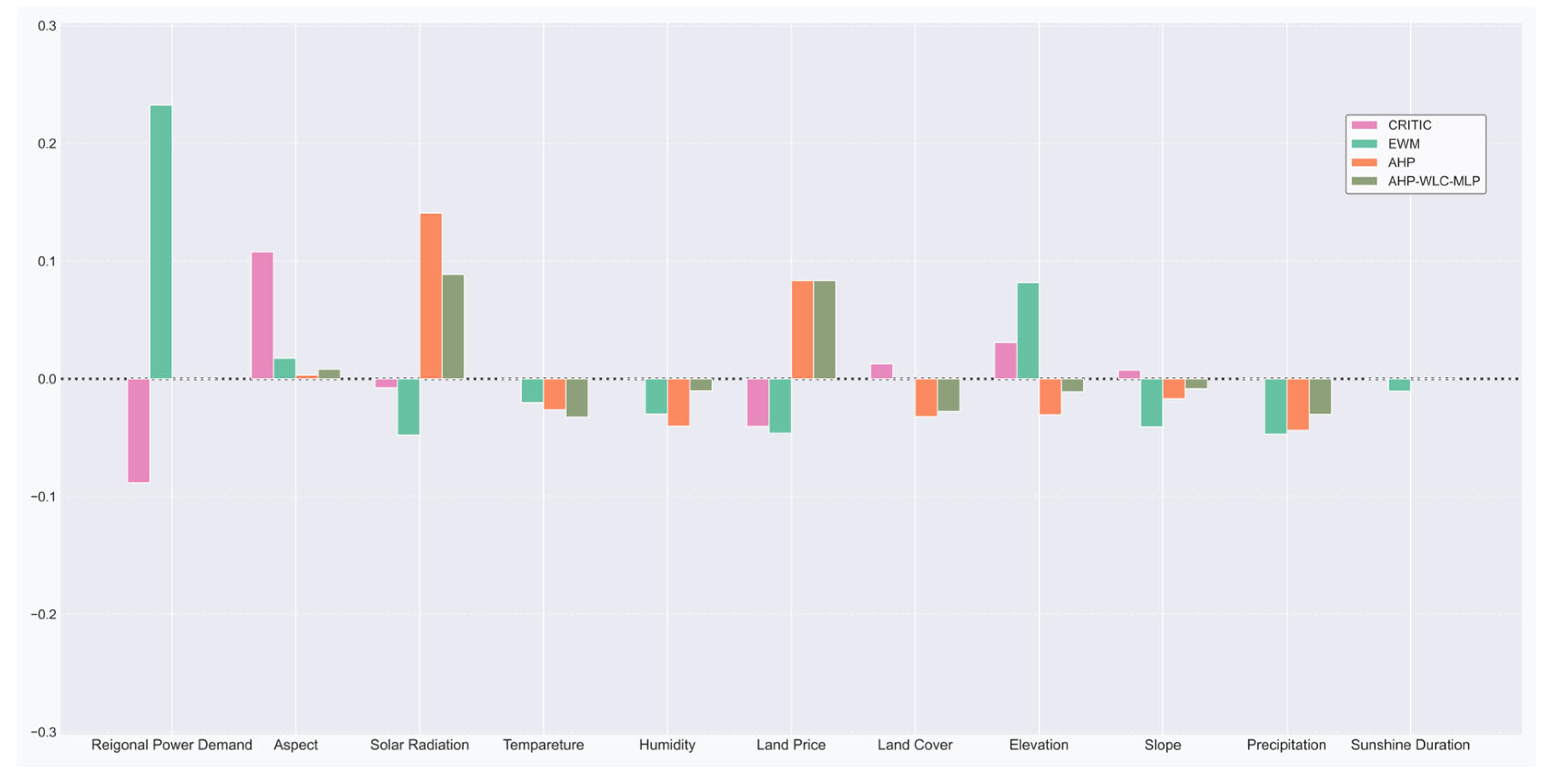
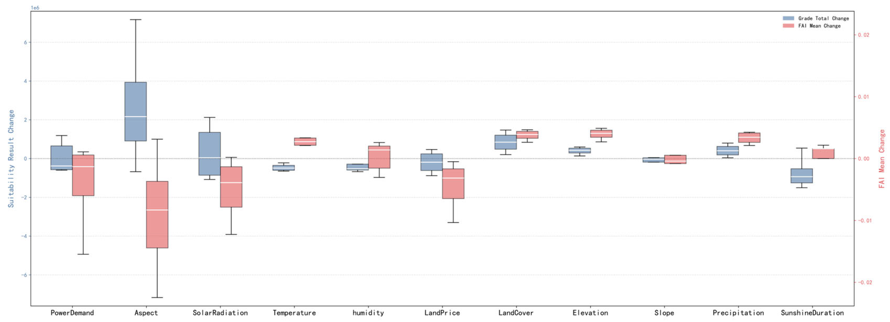
3.7. Sensitivity Analysis
4. Discussion
4.1. Research Implications
- (1)
- Northwest/Southwest China: Prioritize centralized large-scale PV plants in areas with high suitability but low local energy demand and leveraging industrial agglomeration to minimize transmission losses from dispersed small-to-medium installations.
- (2)
- South/Central/East China: Avoid the deployment of large-scale PV plants in regions with limited solar resources; instead, promote distributed PV systems to support localized self-consumption, with excess energy fed into the grid to satisfy regional electricity demands.
- (3)
- North China: Adopt a hybrid development strategy that integrates centralized and distributed systems to optimize solar resource utilization and address regional energy needs.
- (4)
- National Wide: Enhance PV panel conversion efficiency and long-distance transmission capacity, reduce transmission fluctuation losses, and improve solar energy utilization efficiency.
4.2. Comparison with Results from Traditional Methods
4.3. Limitations and Future Directions
5. Conclusions
Author Contributions
Funding
Data Availability Statement
Acknowledgments
Conflicts of Interest
References
- International Renewable Energy Agency. World Energy Transitions Outlook 2024. Available online: https://www.iea.org/reports/world-energy-outlook-2024#overview (accessed on 27 February 2025).
- China Photovoltaic Industry Association. China PV Industry Development RoadMap. Available online: https://english.www.gov.cn/news/202502/27/content_WS67c01568c6d0868f4e8f018b.html (accessed on 27 February 2025).
- International Renewable Energy Agency. Renewable Capacity Statistics 2025. Available online: https://www.irena.org/Publications/2025/Mar/Renewable-capacity-statistics-2025 (accessed on 27 February 2025).
- International Renewable Energy Agency. Country Rankings. 2025. Available online: https://www.irena.org/Data/View-data-by-topic/Capacity-and-Generation/Country-Rankings (accessed on 6 June 2025).
- Energy Institute. Energy Institute Statistical Review of World Energy 2023. Available online: https://www.energyinst.org/statistical-review (accessed on 6 June 2025).
- Zhao, H.; Gu, T.; Tang, J.; Gong, Z.; Zhao, P. Urban flood risk differentiation under land use scenario simulation. iScinece 2023, 26, 106479. [Google Scholar] [CrossRef] [PubMed]
- Mudgal, D.; Pagone, E.; Salonitis, K. Selecting sustainable packaging materials and strategies: A holistic approach considering whole lifecycle and customer preferences. J. Clean. Prod. 2024, 481, 144133. [Google Scholar] [CrossRef]
- Liang, Q.; Zhang, Z.; Su, Y.S. Constructive preference elicitation for multi-criteria decision analysis using an estimate-then-select strategy. Inf. Fusion 2025, 118, 102926. [Google Scholar] [CrossRef]
- Keisler, J.M.; Wells, E.M.; Linkov, I. A Multicriteria Decision Analytic Approach to Systems Resilience. Int. J. Disaster Risk Sci. 2024, 15, 657–672. [Google Scholar] [CrossRef]
- Arán Carrión, J.; Espín Estrella, A.; Aznar Dols, F.; Zamorano Toro, M.; Rodríguez, M.; Ramos Ridao, A. Environmental Decision-Support Systems for Evaluating the Carrying Capacity of Land Areas: Optimal Site Selection for Grid-Connected Photovoltaic Power Plants. Renew. Sustain. Energy Rev. 2008, 12, 2358–2380. [Google Scholar] [CrossRef]
- Fluri, T.P. The Potential of Concentrating Solar Power in South Africa. Energy Policy 2009, 37, 5075–5080. [Google Scholar] [CrossRef]
- Gómez, M.; López, A.; Jurado, F. Optimal Placement and Sizing from Standpoint of the Investor of Photovoltaics Grid-Connected Systems Using Binary Particle Swarm Optimization. Appl. Energy 2010, 87, 1911–1918. [Google Scholar] [CrossRef]
- Sun, Y.; Hof, A.; Wang, R.; Liu, J.; Lin, Y.; Yang, D. GIS-Based Approach for Potential Analysis of Solar PV Generation at the Regional Scale: A Case Study of Fujian Province. Energy Policy 2013, 58, 248–259. [Google Scholar] [CrossRef]
- Ghasemi, G.; Noorollahi, Y.; Alavi, H.; Marzband, M.; Shahbazi, M. Theoretical and Technical Potential Evaluation of Solar Power Generation in Iran. Renew. Energy 2019, 138, 1250–1261. [Google Scholar] [CrossRef]
- Al Garni, H.Z.; Awasthi, A. Solar PV Power Plant Site Selection Using a GIS-AHP Based Approach with Application in Saudi Arabia. Appl. Energy 2017, 206, 1225–1240. [Google Scholar] [CrossRef]
- Almasad, A.; Pavlak, G.; Alquthami, T.; Kumara, S. Site Suitability Analysis for Implementing Solar PV Power Plants Using GIS and Fuzzy MCDM Based Approach. Sol. Energy 2023, 249, 642–650. [Google Scholar] [CrossRef]
- Tercan, E.; Eymen, A.; Urfalı, T.; Saracoglu, B.O. A sustainable framework for spatial planning of photovoltaic solar farms using GIS and multi-criteria assessment approach in Central Anatolia, Turkey. Land Use Policy 2021, 102, 105272. [Google Scholar] [CrossRef]
- Hooshangi, N.; Mahdizadeh Gharakhanlou, N.; Ghaffari Razin, S.R. Evaluation of Potential Sites in Iran to Localize Solar Farms Using a GIS-Based Fermatean Fuzzy TOPSIS. J. Clean. Prod. 2023, 384, 135481. [Google Scholar] [CrossRef]
- Doorga, J.R.S.; Rughooputh, S.D.D.V.; Boojhawon, R. Multi-criteria GIS-based modelling technique for identifying potential solar farm sites: A case study in Mauritius. Renew. Energy 2019, 133, 1201–1219. [Google Scholar] [CrossRef]
- Arnette, A.N.; Zobel, C.W. Spatial Analysis of Renewable Energy Potential in the Greater Southern Appalachian Mountains. Renew. Energy 2011, 36, 2785–2798. [Google Scholar] [CrossRef]
- Omid, A.A.M.; Alimardani, R.; Sarmadian, F. Developing a GIS - Based Fuzzy AHP Model for Selecting Solar Energy Sites in Shodirwan Region in Iran. Int. J. Adv. Sci. Technol. 2014, 68, 37–48. [Google Scholar] [CrossRef]
- Domínguez Bravo, J.; García Casals, X.; Pinedo Pascua, I. GIS Approach to the Definition of Capacity and Generation Ceilings of Renewable Energy Technologies. Energy Policy 2007, 35, 4879–4892. [Google Scholar] [CrossRef]
- Omitaomu, O.A.; Singh, N.; Bhaduri, B.L. Mapping Suitability Areas for Concentrated Solar Power Plants Using Remote Sensing Data. J. Appl. Remote Sens. 2015, 9, 097697. [Google Scholar] [CrossRef]
- Djebbar, R.; Belanger, D.; Boutin, D.; Weterings, E.; Poirier, M. Potential of Concentrating Solar Power in Canada. Energy Procedia 2014, 49, 2303–2312. [Google Scholar] [CrossRef]
- Charabi, Y.; Gastli, A. Integration of Temperature and Dust Effects in Siting Large PV Power Plant in Hot Arid Area. Renew. Energy 2013, 57, 635–644. [Google Scholar] [CrossRef]
- Dagdougui, H.; Ouammi, A.; Sacile, R. A Regional Decision Support System for Onsite Renewable Hydrogen Production from Solar and Wind Energy Sources. Int. J. Hydrogen Energy 2011, 36, 14324–14334. [Google Scholar] [CrossRef]
- Janke, J.R. Multicriteria GIS Modeling of Wind and Solar Farms in Colorado. Renew. Energy 2010, 35, 2228–2234. [Google Scholar] [CrossRef]
- Uyan, M. GIS-Based Solar Farms Site Selection Using Analytic Hierarchy Process (AHP) in Karapinar Region, Konya/Turkey. Renew. Sustain. Energy Rev. 2013, 28, 11–17. [Google Scholar] [CrossRef]
- Noorollahi, Y.; Ghenaatpisheh Senani, A.; Fadaei, A.; Simaee, M.; Moltames, R. A Framework for GIS-Based Site Selection and Technical Potential Evaluation of PV Solar Farm Using Fuzzy-Boolean Logic and AHP Multi-Criteria Decision-Making Approach. Renew. Energy 2022, 186, 89–104. [Google Scholar] [CrossRef]
- Fedakar, H.I.; Dinçer, A.E.; Demir, A. Comparative Analysis of Hybrid Geothermal-Solar Systems and Solar PV with Battery Storage: Site Suitability, Emissions, and Economic Performance. Geothermics 2025, 125, 103175. [Google Scholar] [CrossRef]
- Yu, C.; Lai, X.; Chen, F.; Jiang, C.; Sun, Y.; Zhang, L.; Wen, F.; Qi, D. Multi-Time Period Optimal Dispatch Strategy for Integrated Energy System Considering Renewable Energy Generation Accommodation. Energies 2022, 15, 4329. [Google Scholar] [CrossRef]
- Wang, Y.; Chao, Q.; Zhao, L.; Chang, R. Assessment of Wind and Photovoltaic Power Potential in China. Carbon Neutrality 2022, 1, 1–15. [Google Scholar] [CrossRef]
- Zhang, Y.; Zhao, Z. A Novel Hybrid Multi-Criteria Decision-Making Approach for Solar Photovoltaic Power Plant Site Selection Based on the Quantity and Quality Matching of Resource-Demand. Expert Syst. Appl. 2025, 267, 126014. [Google Scholar] [CrossRef]
- Mokarram, M.; Mokarram, M.J.; Gitizadeh, M.; Niknam, T.; Aghaei, J. A novel optimal placing of solar farms utilizing multi-criteria decision-making (MCDA) and feature selection. J. Clean. Prod. 2020, 261, 121098. [Google Scholar] [CrossRef]
- Ruiz, H.S.; Sunarso, A.; Ibrahim-Bathis, K.; Murti, S.A.; Budiarto, I. GIS-AHP Multi Criteria Decision Analysis for the optimal location of solar energy plants at Indonesia. Energy Rep. 2020, 6, 3249–3263. [Google Scholar] [CrossRef]
- Finn, T.; McKenzie, P. A High-Resolution Suitability Index for Solar Farm Location in Complex Landscapes. Renew. Energy 2020, 158, 520–533. [Google Scholar] [CrossRef]
- Jun, D.; Tian-tian, F.; Yi-sheng, Y.; Yu, M. Macro-Site Selection of Wind/Solar Hybrid Power Station Based on ELECTRE-II. Renew. Sustain. Energy Rev. 2014, 35, 194–204. [Google Scholar] [CrossRef]
- Villacreses, G.; Gaona, G.; Martínez-Gómez, J.; Jijón, D.J. Wind Farms Suitability Location Using Geographical Information System (GIS), Based on Multi-Criteria Decision Making (MCDM) Methods: The Case of Continental Ecuador. Renew. Energy 2017, 109, 275–286. [Google Scholar] [CrossRef]
- Colak, H.E.; Memisoglu, T.; Gercek, Y. Optimal site selection for solar photovoltaic (PV) power plants using GIS and AHP: A case study of Malatya Province, Turkey. Renew. Energy 2020, 149, 565–576. [Google Scholar] [CrossRef]
- Shriki, N.; Rabinovici, R.; Yahav, K.; Rubin, O. Prioritizing Suitable Locations for National-Scale Solar PV Installations: Israel’s Site Suitability Analysis as a Case Study. Renew. Energy 2023, 2023, 105–124. [Google Scholar] [CrossRef]
- Kyomugisha, R.; Muriithi, C.M.; Edimu, M. Multiobjective Optimal Power Flow for Static Voltage Stability Margin Improvement. Heliyon 2021, 7, e08631. [Google Scholar] [CrossRef] [PubMed]
- Varadarajan, M.; Swarup, K.S. Differential Evolutionary Algorithm for Optimal Reactive Power Dispatch. Electr. Power Energy Syst. 2008, 30, 435–441. [Google Scholar] [CrossRef]
- Global Solar Atlas 2.0: Validation Report. World Bank. 2019. Available online: http://documents.worldbank.org/curated/en/507341592893487792 (accessed on 6 June 2025).
- Zhang, J.; Peng, S. China 4 km Spatial Resolution Daily Sunshine Duration Dataset (2000–2020) (Dataset); National Science & Technology Infrastructure of China: Beijing, China, 2025. [Google Scholar] [CrossRef]
- Jing, W. China 1 km Spatial Resolution Monthly Mean Relative Humidity Dataset (2000–2020) (Dataset); National Science & Technology Infrastructure of China: Beijing, China, 2021. [Google Scholar] [CrossRef]
- Peng, S.; Ding, Y.; Liu, W.; Li, Z. 1 Km Monthly Temperature and Precipitation Dataset for China from 1901 to 2017. Earth Syst. Sci. Data 2019, 11, 1931–1946. [Google Scholar] [CrossRef]
- National Centers for Environmental Information (NCEI). Global Surface Summary of the Day–GSOD. Available online: https://www.ncei.noaa.gov/access/metadata/landing-page/bin/iso?id=gov.noaa.ncdc:C00516 (accessed on 3 August 2023).
- NASADEM: Creating a New NASA Digital Elevation Model and Associated Products | NASA Earthdata. Available online: https://www.earthdata.nasa.gov/about/competitive-programs/measures/new-nasa-digital-elevation-model (accessed on 1 May 2025).
- 1:1 Million Public Edition Fundamental Geographic Information Data (2021). Available online: https://www.webmap.cn/commres.do?method=result100w (accessed on 3 August 2023).
- Yang, J.; Huang, X. The 30 m annual land cover dataset and its dynamics in China from 1990 to 2019. Earth Syst. Sci. Data 2021, 13, 3907–3925. [Google Scholar] [CrossRef]
- China Land Supply. Available online: https://www.ceicdata.com/en/china/land-supply/land-supply-ytd (accessed on 1 April 2025).
- Chen, J.; Gao, M.; Cheng, S.; Hou, S.; Song, M.; Liu, X.; Liu, Y. Global 1 km × 1 km gridded revised real gross domestic product and electricity consumption during 1992–2019 based on calibrated nighttime light data. Sci. Data 2022, 9, 202. [Google Scholar] [CrossRef]
- Lyu, X.; Li, X.; Wei, H.; Wu, J.; Dang, D.; Zhang, C.; Wang, K.; Lou, A. Mapping of Utility-Scale Solar Panel Areas From 2000 to 2022in China Using Google Earth Engine. IEEE J. Sel. Top. Appl. Earth Obs. Remote Sens. 2024, 17, 18083–18095. [Google Scholar] [CrossRef]
- Photovoltaic Power Station Design Specifications. Available online: https://www.mohurd.gov.cn/gongkai/zc/wjk/art/2024/art_96bd1b03e8d54760b4dff9ad60352ddc.html (accessed on 1 April 2025).
- China Photovoltaic Industry Association. 2022–2023 China Photovoltaic Industry Annual Report. 2023. Available online: https://www.chinapv.org.cn/Industry/resource_1285.html (accessed on 1 April 2025).
- China Photovoltaic Industry Association. 2020–2021 China Photovoltaic Industry Annual Report. 2021. Available online: https://www.chinapv.org.cn/Industry/resource_1012.html (accessed on 1 April 2025).
- China Photovoltaic Industry Association. 2019–2020 China Photovoltaic Industry Annual Report. 2020. Available online: https://www.chinapv.org.cn/Industry/resource_821.html (accessed on 1 April 2025).
- China Photovoltaic Industry Association. 2018–2019 China Photovoltaic Industry Annual Report. 2019. Available online: https://www.chinapv.org.cn/Industry/resource_820.html (accessed on 1 April 2025).
- China Photovoltaic Industry Association. 2017–2018 China Photovoltaic Industry Annual Report. 2019. Available online: https://www.chinapv.org.cn/Industry/resource_584.html (accessed on 1 April 2025).
- Saaty, T.L. A Scaling Method for Priorities in Hierarchical Structures. J. Math. Psychol. 1977, 15, 234–281. [Google Scholar] [CrossRef]
- Rumelhart, D.E.; Hinton, G.E.; Williams, R.J. Learning Representations by Back-Propagating Errors. Nature 1986, 323, 533–536. [Google Scholar] [CrossRef]
- Kingma, D.P.; Ba, J.L. Adam: A Method for Stochastic Optimization, Ver. 9. arXiv 2014, arXiv:1412.6980. [Google Scholar]
- Loshchilov, I.; Hutter, F. SGDR: Stochastic Gradient Descent with Warm Restarts, Ver. 1. arXiv 2016, arXiv:1608.03983. [Google Scholar]
- Lundberg, S.; Lee, S. A Unified Approach to Interpreting Model Predictions, Ver. 1. arXiv 2017, arXiv:1705.07874. [Google Scholar]


| Criteria | Sub-Criteria | Attribute | Threshold | Type | Source |
|---|---|---|---|---|---|
| Climatic | Solar Radiation | common | – | Maximize | a |
| Sunshine Duration | common | – | Maximize | b | |
| Humidity | common | – | Minimize | c | |
| Precipitation | common | – | Minimize | a | |
| Temperature | common | – | Minimize | d | |
| Orography | Elevation | common/Exclusion | 6000 m | Maximize | e |
| Slope | common/Exclusion | 35° | Minimize | e | |
| Aspect | common | – | Maximize | e | |
| Location | Proximity to Reserve | Exclusion | 1000 m | – | f |
| Land Cover | common/Exclusion | 0 | Maximize | g | |
| Economic | Land Price | common | – | Minimize | h |
| Regional Power Demand | common | – | Maximize | i |
| Sub-Criteria | Limitation | Grade |
|---|---|---|
| Land Cover | Barren | 5 |
| Grassland | 4 | |
| Shrub and Impervious | 3 | |
| Forest | 2 | |
| Wetland | 1 | |
| Water and Snow/Ice and Cropland | 0 | |
| Aspect | South | 5 |
| Southeast and Southwest | 4 | |
| East and West | 2 | |
| Northeast and Northwest | 1 | |
| North | 0 |
| Importance | Definition |
|---|---|
| 1 | The two criteria are of equal importance |
| 3 | Somewhat more importance of the former over the latter |
| 5 | Much more importance of the former over the latter |
| 7 | Very much more importance of the former over the latter |
| 9 | Absolutely more importance of the former over the latter |
| 2, 4, 6, 8 | Intermediate values |
| Multiplicative Inverses for 1–9 | Reciprocal Importance in Transposed Comparisons |
| Criteria | Temperature | Precipitation | Humidity | Solar Radiation | Elevation | Aspect | Slope | Sunshine Duration | Land Cover | Land Price | Regional Power Demand |
|---|---|---|---|---|---|---|---|---|---|---|---|
| Temperature | 1.000 | 3.000 | 0.333 | 0.111 | 1.000 | 0.143 | 0.200 | 0.143 | 0.333 | 0.111 | 0.111 |
| Precipitation | 0.333 | 1.000 | 0.333 | 0.111 | 0.333 | 0.143 | 0.143 | 0.143 | 0.200 | 0.143 | 0.111 |
| Humidity | 3.000 | 3.000 | 1.000 | 0.111 | 1.000 | 0.200 | 0.333 | 0.200 | 1.000 | 0.143 | 0.111 |
| Solar Radiation | 9.000 | 9.000 | 9.000 | 1.000 | 9.000 | 5.000 | 7.000 | 5.000 | 9.000 | 3.000 | 2.000 |
| Elevation | 1.000 | 3.000 | 1.000 | 0.111 | 1.000 | 0.200 | 0.333 | 0.200 | 1.000 | 0.143 | 0.143 |
| Aspect | 7.000 | 7.000 | 5.000 | 0.200 | 5.000 | 1.000 | 3.000 | 1.000 | 3.000 | 0.200 | 0.143 |
| Slope | 5.000 | 7.000 | 3.000 | 0.143 | 3.000 | 0.333 | 1.000 | 0.333 | 3.000 | 0.143 | 0.143 |
| Sunshine Duration | 7.000 | 7.000 | 5.000 | 0.200 | 5.000 | 1.000 | 3.000 | 1.000 | 3.000 | 0.200 | 0.167 |
| Land Cover | 3.000 | 5.000 | 1.000 | 0.111 | 1.000 | 0.333 | 0.333 | 0.333 | 1.000 | 0.200 | 0.143 |
| Land Price | 9.000 | 7.000 | 7.000 | 0.333 | 7.000 | 5.000 | 7.000 | 5.000 | 5.000 | 1.000 | 0.333 |
| Regional Power Demand | 9.000 | 9.000 | 9.000 | 0.500 | 7.000 | 7.000 | 7.000 | 6.000 | 7.000 | 3.000 | 1.000 |
| Criteria | Weight (%) | Threshold for Unsuitability |
|---|---|---|
| Temperature | 1.623 | >23.00 °C |
| Precipitation | 1.14 | >2000.00 mm/year |
| Humidity | 2.496 | >90.00% |
| Solar Radiation | 27.517 | <1000.00 kWh/m2 |
| Elevation | 2.311 | <0.00 m |
| Aspect | 7.848 | <1.00 |
| Slope | 4.836 | >7.00° |
| Sunshine Duration | 7.959 | <1200 h/year |
| Land Cover | 3.026 | <0.25 |
| Land Price | 16.949 | >6176.00 yuan |
| Regional Power Demand | 24.295 | <61,159,751.74 kWh |
| Criteria | Threshold | Clustering Centroid | Expert Threshold | |||||
|---|---|---|---|---|---|---|---|---|
| Class 1 | Class2 | Class 3 | Centroid | Centroid | Centroid | Centroid | ||
| Temperature (°C) | 13.89 | 8.96 | 4.93 | 17.17 | 10.60 | 7.32 | 2.54 | 23 |
| Precipitation (mm) | 1002.42 | 513.61 | 344.03 | 1401.44 | 603.39 | 443.78 | 244.27 | 2000 |
| Humidity (%) | 63.80 | 53.14 | 44.27 | 69.83 | 57.76 | 48.53 | 40.01 | 90 |
| Solar Radiation (kWh/m2) | 1373.33 | 1512.82 | 1705.44 | 1306.91 | 1439.76 | 1585.88 | 1825.00 | 1000 |
| Elevation (m) | 567.47 | 928.26 | 2680.65 | 412.85 | 722.09 | 1134.42 | 4226.88 | 0 |
| Aspect | – | – | – | 1.84 | 2.40 | 3.20 | 4.40 | 1.00 |
| Slope (°) | 3.40 | 2.62 | 1.82 | 3.78 | 3.01 | 2.24 | 1.40 | 7 |
| Sunshine Duration (h) | 921.06 | 2826.59 | 3197.53 | 1310.10 | 2532.02 | 3121.16 | 3273.90 | 1200 |
| Land Cover | 1.00 | 2.35 | 3.85 | 0.80 | 1.20 | 3.50 | 4.20 | 0.25 |
| Land Price (yuan) | 362.02 | 127.01 | 57.90 | 638.44 | 205.27 | 78.59 | 42.66 | 6176 |
| Regional Power Demand (kWh) | 3.67 × 10⁸ | 8.40 × 10⁸ | 2.62 × 10⁹ | 2.69 × 10⁸ | 5.00 × 10⁸ | 1.41 × 10⁹ | 4.89 × 10⁹ | 6.11 × 10⁷ |
| Criteria | Weight (%) |
|---|---|
| Temperature | 1.01 |
| Precipitation | 2.48 |
| Humidity | 5.50 |
| Solar Radiation | 22.32 |
| Elevation | 4.27 |
| Aspect | 8.36 |
| Slope | 5.69 |
| Sunshine Duration | 6.12 |
| Land Cover | 3.47 |
| Land Price | 16.95 |
| Regional Power Demand | 23.83 |
| Algorithm | CH Index | Sample Distribution | |||
|---|---|---|---|---|---|
| Class 1 | Class 2 | Class 3 | Class 4 | ||
| I-KMEANS* | 2,818,164 | 543,715 | 1,413,679 | 1,832,426 | 735,331 |
| Isotonic Regression | 1,186,760 | 453,400 | 1,579,154 | 1,484,735 | 1,007,862 |
| Natural Break | 1,010,094 | 447,104 | 1,351,661 | 2,324,195 | 402,191 |
| Quantile Method | 597,613 | 1,132,660 | 666,369 | 2,103,086 | 623,036 |
| Algorithm | CH Index | Sample Distribution | |||
|---|---|---|---|---|---|
| Class 1 | Class 2 | Class 3 | Class 4 | ||
| Unconstrained | 3,317,482 | 638,434 | 1,927,121 | 1,288,756 | 670,840 |
| I-KMEANS* | 2,818,164 | 543,715 | 1,413,679 | 1,832,426 | 735,331 |
| Isotonic Regression only | 2,580,042 | 631,929 | 1,295,325 | 1,857,809 | 740,088 |
| Sort only | 2,041,104 | 581,146 | 1,346,833 | 1,902,915 | 694,257 |
Disclaimer/Publisher’s Note: The statements, opinions and data contained in all publications are solely those of the individual author(s) and contributor(s) and not of MDPI and/or the editor(s). MDPI and/or the editor(s) disclaim responsibility for any injury to people or property resulting from any ideas, methods, instructions or products referred to in the content. |
© 2025 by the authors. Licensee MDPI, Basel, Switzerland. This article is an open access article distributed under the terms and conditions of the Creative Commons Attribution (CC BY) license (https://creativecommons.org/licenses/by/4.0/).
Share and Cite
Liao, Y.; Miao, S.; Fan, W.; Liu, X. A Novel Hybrid Fuzzy Comprehensive Evaluation and Machine Learning Framework for Solar PV Suitability Mapping in China. Remote Sens. 2025, 17, 2070. https://doi.org/10.3390/rs17122070
Liao Y, Miao S, Fan W, Liu X. A Novel Hybrid Fuzzy Comprehensive Evaluation and Machine Learning Framework for Solar PV Suitability Mapping in China. Remote Sensing. 2025; 17(12):2070. https://doi.org/10.3390/rs17122070
Chicago/Turabian StyleLiao, Yanchun, Shuangxi Miao, Wenjing Fan, and Xingchen Liu. 2025. "A Novel Hybrid Fuzzy Comprehensive Evaluation and Machine Learning Framework for Solar PV Suitability Mapping in China" Remote Sensing 17, no. 12: 2070. https://doi.org/10.3390/rs17122070
APA StyleLiao, Y., Miao, S., Fan, W., & Liu, X. (2025). A Novel Hybrid Fuzzy Comprehensive Evaluation and Machine Learning Framework for Solar PV Suitability Mapping in China. Remote Sensing, 17(12), 2070. https://doi.org/10.3390/rs17122070