Article

Twilight Near-Infrared Radiometry for Stratospheric Aerosol Layer Height

by
Lipi Mukherjee
1,2,*,
Dong L. Wu
2,
Nader Abuhassan
1,3,4,
Thomas F. Hanisco
3,
Ukkyo Jeong
5,
Yoshitaka Jin
6,
Thierry Leblanc
7,
Bernhard Mayer
8,
Forrest M. Mims III
9,
Isamu Morino
6,
Tomohiro Nagai
10,
Stephen Nicholls
11,12,
Richard Querel
13,
Tetsu Sakai
10,
Ellsworth J. Welton
14,
Stephen Windle
15,
Peter Pantina
2,11 and
Osamu Uchino
10
1
Goddard Earth Sciences Technology and Research (GESTAR-II), University of Maryland, Baltimore County, Baltimore, MD 21228, USA
2
Climate and Radiation Lab, NASA Goddard Space Flight Center, Greenbelt, MD 20770, USA
3
Atmospheric Chemistry and Dynamics Laboratory, NASA Goddard Space Flight Center, Greenbelt, MD 20770, USA
4
Sciglob Instrument and Services, 9881 Broken Land Pkwy, Columbia, MD 21046, USA
5
Major of Geomatics Engineering, Division of Earth and Environmental System Sciences, Daeyeon Campus, Pukyong National University, Busan 48513, Republic of Korea
6
National Institute for Environmental Studies, 16-2 Onogawa, Tsukuba 305-8506, Ibaraki, Japan
7
Jet Propulsion Laboratory, California Institute of Technology, Wrightwood, CA 92397, USA
8
Lehrstuhl fuer Experimentelle Meteorologie, Ludwig-Maximilians-Universitaet, Theresienstrasse 37, 80333 Munich, Germany
9
Geronimo Creek Atmospheric Monitoring Station, Seguin, TX 78155, USA
10
Meteorological Research Institute, Japan Meteorological Agency, 1-1 Nagamine, Tsukuba 305-0052, Ibaraki, Japan
11
Science Systems and Applications, Inc. (SSAI), Lanham, MD 20706, USA
12
Mesoscale Atmospheric Process Lab, Boulder, CO 80301, USA
13
National Institute of Water & Atmospheric Research Ltd. (NIWA), Lauder 9377, New Zealand
14
Mesoscale Atmospheric Processes, NASA Goddard Space Flight Center, Greenbelt, MD 20770, USA
15
Department of Atmospheric and Oceanic Science, University of Maryland, College Park, MD 20742, USA
*
Author to whom correspondence should be addressed.
Remote Sens. 2025, 17(12), 2071; https://doi.org/10.3390/rs17122071
Submission received: 7 March 2025 / Revised: 27 May 2025 / Accepted: 2 June 2025 / Published: 16 June 2025

Abstract

The impact of stratospheric aerosols on Earth’s climate, particularly through atmospheric heating and ozone depletion, remains a critical area of atmospheric research. While satellite data provide valuable insights, independent validation methods are necessary for ensuring accuracy. Twilight near-infrared (NIR) radiometry offers a promising approach for investigating aerosol properties, such as optical depth and layer height, at high altitudes. This study aims to evaluate the effectiveness of twilight radiometry in corroborating satellite data and assessing aerosol characteristics. Two methods based on twilight radiometry—the color ratio and the derivative method—are employed to derive the aerosol layer height and optical depth. Radiances at 450, 550, 762, 775, and 1050 nm wavelengths are analyzed at varying solar zenith angles, using zenith viewing geometry for consistency. Comparisons of aerosol optical depths (AODs) between Research Pandora (ResPan) and AErosol RObotic NETwork (AERONET) data (R = 0.99) and between ResPan and Modern-Era Retrospective analysis for Research and Applications (MERRA-2) data (R = 0.86) demonstrate a strong correlation. Twilight ResPan data are also used to estimate the aerosol layer height, with results in good agreement with SAGE and lidar measurements, particularly following the Hunga Tonga eruption in Lauder, New Zealand. The simulation database, created using the libRadtran DISORT and Monte Carlo packages for daylight and twilight calculations, is capable of detecting AODs as low as 10−3 using the derivative method. This work highlights the potential of twilight radiometry as a simple, cost-effective tool for atmospheric research and satellite data validation, offering valuable insights into aerosol dynamics at stratospheric altitudes.

1. Introduction

Twilight influences life on Earth, with its illumination varying by latitude and season due to the atmospheric density [1]. It affects plant growth and blooming times, while also providing cooler temperatures and favorable hunting conditions for wildlife. The low-light conditions during this transitional period, with fish coming to the surface of the water to nourish themselves before going back to deeper waters, [2,3], make it an ideal time for fishing activities. As such, twilight plays a critical role in the ecosystems of many regions, influencing both natural processes and human activities.
Twilight can be classified into three distinct phases, each marked by a specific angle of solar depression below the horizon [4]. Civil twilight, when the Sun is between 0° and 6° below the horizon, is good for landscape imaging. Next is nautical twilight, which is when the Sun is between 6° and 12° below the horizon. During this time, some major stars are visible, which help the sailors in navigation. The last is astronomical twilight, which is when the geometric center of the Sun is between 12° and 18°. Astronomers use the astronomical twilight time to observe stars or planets that appear as bright points. It should be noted that the illumination level of different twilight periods depends not only on the depression of the Sun but also on the presence of clouds.
Twilight sky brightness is caused by sunlight scattered by molecules, aerosols, and ozone in a thin volume of air above the momentary height of Earth’s shadow during sunset/sunrise, as shown in Figure 1. This phenomenon is measured through twilight radiometry (TRM), a technique that has been employed since the early 19th century to study the vertical optical properties of the atmosphere. In an attempt to record daylight illumination, the study was extended to the Sun’s depression angles of 2 ° , 3 ° , and 6 ° using a visual photometer [5,6]. Subsequently, the shortening of civil twilight in the presence of clouds was investigated [6]. An increase in twilight sky brightness due to forest fires was also observed [6]. The measurements were made using a Weber photometer with the Sun at a depression of 8 ° . A wedge photometer measured twilight intensity at Sun depression angles of 8 . 5 ° to 13 . 5 ° , establishing the relationship between decreasing intensity and increasing solar depression [6].
Despite these foundational studies, several critical gaps in the understanding of twilight brightness remained unresolved. One significant challenge was the difficulty in comparing twilight measurements across different observers due to inconsistent methodologies and a lack of standardized absolute twilight intensity data. As a result, the connection between twilight brightness and the optical properties of Earth’s atmosphere remained understudied. Additionally, the limited range of solar depression angles investigated further constrained the depth of these studies. These issues persisted even as researchers like [6] expanded their observations, using both visual photometers and photoelectric cells, and presented data on air density as a function of altitude. These methods were later applied to detect aerosol and dust layers in the atmosphere by measuring variations in twilight intensity [7,8]. Their work concluded that twilight intensity could be a reliable method for observing dust in the atmosphere. Furthermore, while some research suggested that stratospheric aerosols could influence twilight brightness—particularly after volcanic eruptions [9,10,11,12,13]—there was insufficient observational evidence to quantify this impact reliably. Earlier measurements were often challenged by inconsistent methodologies and limited observational reach for studying stratospheric aerosols.
In addition to these challenges, stratospheric aerosols have been a key focus in Earth science due to their significant impact on climate. These aerosols influence the radiative balance [14], contribute to stratospheric warming, accelerate ozone depletion through chemical reactions, and disrupt global stratospheric dynamics [15]. They are also believed to negatively impact nitrogen dioxide, which plays a crucial role in various stratospheric chemical cycles [16]. Although the stratosphere contains only 17% of the atmosphere’s mass, its instability can have a profound influence on the troposphere, which in turn affects surface conditions. Stratospheric aerosols, such as condensed aerosols and mineral dust, can influence climate change both regionally and globally during events of high aerosol injection, such as volcanic eruptions [17].
To improve our understanding of these aerosols, many satellite-borne monitoring instruments are used, providing global-scale data. The Stratospheric Aerosol Measurement (SAM) and later SAM II instruments were developed to analyze stratospheric aerosol data for polar regions. The SAGE missions (SAGE I, II, and III) are remote sensing instruments that use the solar occultation technique to study important atmospheric constituents like aerosols, ozone, and water vapor [18,19,20,21]. However, the global-scale data provided by these instruments must be validated using other methods, such as in situ sampling (balloon-borne) and remote scattering measurements like ground-based lidars [22]. Stratospheric aerosols also impact twilight sky brightness. Consequently, measurements of twilight sky brightness caused by aerosol scattering can serve as an alternative method to corroborate satellite-based findings. This serves as the primary motivation for the current study.
The challenges of previous twilight radiometry research are addressed by employing advanced radiative transfer modeling techniques and high-quality observational data. All calculations are performed using the zenith viewing geometry. Compared to direct-Sun geometry, the zenith view provides measurements during twilight and is particularly advantageous for retrieving near-surface species like nitrogen dioxide and formaldehyde [23], especially in thin and moderate cloud conditions when direct Sun measurements are difficult to achieve. Additionally, this viewing geometry can help differentiate between ground surfaces, as will be discussed later. The study of twilight has been conducted using a Monte Carlo-based radiative transfer (RT) model from libRadtran [24], with data obtained from the ResPan spectroradiometer (Reserach Pandora), similar to the one discussed in [25]. The technique is employed to ascertain two key aerosol properties: aerosol optical depth (AOD) and aerosol layer height (ALH). Several key findings are presented in this study.
AOD and ALH are critical parameters for understanding climate dynamics. AOD is an optical parameter of aerosols, widely used as an indicator of air pollution. It reflects how much direct sunlight is blocked by air pollutants (such as dust, smoke, etc.). This dimensionless quantity can impact air quality, climate change, human health, and the balance between incoming solar energy and outgoing radiation from Earth [26]. Knowledge of ALH is essential for determining the impact of aerosols at different vertical heights of the atmosphere, which, in turn, influences the formation and lifecycle of clouds [27,28]. ALH plays a key role in the direct and indirect radiative forcing of aerosols, which is required for calculating Earth’s energy budget [29,30,31]. Moreover, it can help identify and trace the long-range transport of aerosols, shedding light on their lifecycle and enabling the monitoring of air quality to forecast severe air pollution events [32]. The retrieval of ALH depends on the wavelength observed, as detailed in previous studies [10,11]. In the discussion section, the calculated minimum heights corresponding to different observational wavelengths are presented.
This study extends previous work by utilizing twilight radiometry beyond 1000 nm, allowing for more precise aerosol layer height detection. By integrating advanced radiative transfer modeling techniques and improved observational datasets, a more robust method for stratospheric aerosol analysis has been presented. Previous studies, such as [33], proposed a simple analytical expression for twilight brightness. This expression has now been compared against radiative transfer (RT) simulations under clear sky conditions, both including and excluding ozone, as as discussed later. All RT calculations were performed using the libRadtran package [24,34]. For RT simulations in twilight (i.e., for solar zenith angle ( 90 ° < SZA < 100 ° ), the Monte Carlo solver MYSTIC has been used [24]. It is a fully spherical code that takes the spherical geometry of the Earth into account without simplifying assumptions [35]. With the help of this model, layer height information at different wavelengths can be investigated and discussed. Comparisons of AODs on different days between the ResPan instrument and collocated AERONET (AErosol RObotic NETwork) measurements during daylight, at various SZAs, are presented in Section 4. Additionally, comparisons between ResPan and MERRA-2’s (Modern Era Retrospective Analysis for Research and Applications-2) [36] AOD at 550 nm are also discussed. For daylight conditions (i.e., for SZA < 90 ° ), the DISORT RT code (pseudospherical from 80 ° < SZA < 90 ° ) from the libRadtran package [24] has been used. Furthermore, the impact of the Hunga Tonga volcanic eruption on aerosol loading has been explored, with data from the ResPan instrument at the Lauder site used to study aerosol layer heights in comparison to SAGE and lidar measurements.
The paper is organized as follows: Section 2 describes the adopted method; Section 3 outlines the data used; Section 4 presents the results; Section 5 provides an analysis of the results; Section 6 summarizes the conclusions reached of this study; Appendix A provides the analytical methods, and Appendix B provides the calibration procedures applied in this study.

2. Twilight Radiometry

Twilight radiometry provides a method for estimating aerosol properties based on light scattering during twilight conditions. When the Sun is below the horizon, the upper part of Earth’s atmosphere is illuminated, and the lower part is partly obscured by Earth’s shadow. The scattering due to molecules as well as ozone and aerosol particles above this boundary causes the twilight sky brightness. The lowest atmospheric layer, which is the densest, contributes most to the scattering and can thus be measured by detecting the shadow height corresponding to the twilight SZA. The twilight radiometry method can cover a wide range of altitudes. Volcanic eruptions enhance the stratospheric aerosol layer loading at certain altitudes. The twilight brightness method, as discussed previously in many works [10,11,12,13,37,38], has been used to study and retrieve the optically active constituents of Earth’s atmosphere.
Figure 1 shows the geometry of the two cases studied in this work. Daylight occurs when SZA < 90 ° (when solar rays passes the Earth’s atmosphere), and twilight occurs when the SZA > 90 ° (when solar rays graze Earth’s surface). Both cases use a zenith viewing direction where R e is the radius of the Earth, θ is the depression angle, and I 0 ( λ ) is the incident intensity. The geomteric shadow height (z) is from the surface of the Earth where the line of sight and rays grazing the Earth meet, as shown in Figure 1. When this ray hits the aerosol layer (red), this particular height becomes key to the aerosol layer height information. In the diagram, the ozone layer is shown in blue. As solar light passes the Earth’s atmosphere, it undergoes wavelength-dependent attenuation and molecular scattering. Additionally, absorption due to water vapor and ozone is present as well. Therefore, the geometric shadow is defined as the shadow height which Earth would cast if it had no atmosphere [39]. In previous works, the effective height of Earth’s shadow derived from the visible range included a screening height added to the geometric shadow height. An expression for the effective Earth’s shadow height was suggested as z + ( 20 / sin θ ) km, and 20 / sin θ is the screening height derived by [40]. Later, it was suggested to add 11 km for 450 nm and 3 km for 650 nm to account for the screening height [39,40].
The geomteric Earth’s shadow height, excluding the screening height, z, (as shown in Figure 1) for zenith viewing can be computed as
z = R e ( s e c θ 1 ) ,
where R e and θ are the same as discussed before. If longer wavelengths (>650 nm) are used for observation, then the Earth’s shadow height would be very close to the geometric shadow height of the lowest grazing rays also mentioned in earlier work [7]. This is confirmed by computation done using various wavelengths, where longer wavelengths are able to detect the aerosol layer height well, which is close to the geometrical shadow height of the lowest grazing rays, as shown as discussed further in Section 4 and Section 5. Early twilight studies initially used wavelengths up to around 650 nm. It was not until later that longer wavelengths, extending to approximately 800 nm, were introduced into twilight observations [12]. This study, to the best of the authors’ knowledge, represents the first application of twilight radiometry beyond 1000 nm wavelengths, providing new insights into aerosol layer heights at stratospheric altitudes. The deductions are compared against other lower wavelengths.
An expression for the brightness of the sky with the Earth’s atmosphere both with pure air and air with ozone was presented in the work [33]. The expression for clear sky with and without ozone was verified first and then subsequently compared against the radiance calculated by the Monte Carlo RT code [24]. The brightness expressions are given in the appendix (Appendix A), and the comparison outcomes are presented in the result (Section 4). The impacts of single versus multiple scattering at different ranges of wavelength are also highlighted.
To study the relationship between aerosol properties (AOD and ALH), the RT code was simulated at different SZAs and wavelengths. The wavelengths 450, 550, 762, 775, and 1050 nm were used as part of this study. For the aerosol model, Gaussian-shaped stratospheric aerosol layers have been implemented in the model atmosphere at mean altitudes, 5, 10, 15, 20, 30, and 40 km with variance of the distribution of 0.85 (close to 1). A minimum mean altitude of 5 km was chosen in this study to explore the limits of the twilight radiometry method. The stratospheric aerosol optical thickness (at λ = 550 nm) ranged from values of τ = 0.003, 0.005, 0.008, and 0.01. The Sun was treated as a point source, and convolution of the solar zenith angle with half a degree was not performed.
This work used the ratio of intensity/radiance at two wavelengths, also known as the color ratio method, to identify aerosol properties (AOD and ALH). In the past, this method has been successfully used to detect the AOD [37,38] using different wavelength ratios. The method is based on the characteristic wavelength dependency of scattering by particles. For instance, Rayleigh scattering predominates at shorter wavelengths, whereas aerosol scattering is more significant at longer wavelengths. Based on this fact, the ratio of the intensities at 775 nm and 450 nm is found to be useful to infer the aerosols’ ALH and AOD information. The oxygen-A band is commonly used to retrieve aerosol height information [41,42,43,44,45]. Oxygen is a well-mixed gas in the atmosphere, and because of its pressure dependence, it can provide reliable vertical information regarding aerosols [45]. This is possible because the oxygen-A band’s absorption gets modified by the multiple scattering events caused by aerosols at various altitudes [43]. The oxygen-A band wavelength has been used for remote sensing with satellite-based as well as ground-based instruments [46]. Particularly, the wavelength 762 nm was chosen from the oxygen-A band. The relationship between the ratio of 775 nm and 450 nm and difference of 775 and 762 nm has been explored. It has been found to provide consistent and reliable information about ALH as well as AOD. The band at 550 nm was used to inspect the aerosol information, as it corresponds to the peak of the solar spectrum and the mid visible range where the radiative effect is highest [47]. The Ångström exponent equation is
τ ( λ )   =   β λ α
where τ ( λ ) is the aerosol optical depth (AOD) at wavelength λ , β is the turbidity coefficient, and α is the Ångström exponent. If AODs at two wavelengths are known ( λ 1 and λ 2 ) using Equation (2), α can be calculated as
α   =   ln τ ( λ 1 ) τ ( λ 2 ) ln λ 1 λ 2
Thereafter, the AOD at an unknown wavelength ( λ ) can be obtained as
τ ( λ )   =   τ ( λ 1 ) λ λ 1 α
AERONET’s spectral AODs at 440 and 675 nm were used to obtain the Ångström exponent and the AOD at 550 nm using Equations (2)–(4), which was then compared against MERRA-2’s AOD at 550 nm. The twilight method was applied to show that the aerosol layer height as low as 5 km can be detected with the help of longer observing wavelengths. The height limitation is imposed by the attenuation of atmospheric layers closer to the Earth’s surface. The SZAs (around 94 ° ) corresponding to heights of 20 and 30 km have been used to demonstrate the twilight theory. Direct-Sun measurements perform well for SZA measurements until 80 ° , but zenith-sky measurements allow for extended spectral measurements, which help provide aerosol height information. Ordinarily, during twilight with a non-turbid atmosphere, the intensity decreases rapidly with increase in height and with an increase in SZA. However, the presence of the aerosol layer leads to increased scattering, which manifests as a peak in the intensity versus SZA plot. This method of detecting the aerosol layer was first proposed in [40]. Following this concept, the logarithmic gradient of intensity q ( λ , z ) (where intensity is measured in relative units) calculated from the rate of change in intensity with height, is a key method to detect the aerosol layers based on their scattering properties:
q ( λ , z ) = d logI λ / dz = d I λ / ( I λ dz ) .
The z value is the vertical height or Earth’s shadow height corresponding to the solar depression angle θ , as used in Figure 1, and d I λ is the corresponding change in scattered intensity. As mentioned before, the scattered intensity also depends on the wavelength of observation. Molecular scattering and ozone absorption diminish with increasing wavelength, which makes aerosol scattering a relatively more significant contributor. Consequently, longer wavelengths in the near-infrared range are particularly useful for retrieving aerosol properties. The atmospheric refraction has been neglected in this work.
In previous studies of twilight simulations, the pseudospherical DISORT RT code was used, which incorporates Chapman functions to account for the Earth’s curvature [12,37]. However, it was realized that for higher SZAs or a low Sun, the pseudospherical correction is not sufficient. In such cases, a fully spherical solver—such as a Monte Carlo model—is required [13,24,35]. The models used in this work are from the libRadtran package, which is a library of various RT routines and programs [24,34]. The Total and Spectral Solar Irradiance Sensor (TSIS) solar spectrum has been used for the solar input [48]. For twilight simulations starting from a solar zenith angle (SZA) of 90 ° , the MYSTIC solver is used [49]. For SZAs between 80 ° and 90 ° , the DISORT solver with a pseudospherical approximation is preferred, as it is significantly faster than MYSTIC while still providing comparable accuracy when the Sun is above the horizon.
For RT simulation with SZA 80 ° , the DISORT solver is used [50]. The Monte Carlo method is subject to statistical noise, but MYSTIC does not use any simplifying assumptions or approximations to solve the radiative transfer equation, as shown in [51]. Therefore, it does not introduce any bias, which has been confirmed by various comparisons with independent radiative transfer solvers and by comparison with observations. The statistical noise in the Monte Carlo based RT simulations were reduced by using 1 × 10 9 photons. Moreover, the derivative method used in the paper would not be affected by a constant offset factor, since here we calculate dI/I.
For the Greenbelt location, an urban surface was adopted in the model, while grassland was used as the corresponding surface type for the Lauder location.
Figure 2 shows the background aerosol, Rayleigh, and ozone profile used in the RT model as part of this work [24]. The model employs the US Standard Atmosphere 1976, as implemented in the libradtran package [24]. The atmospheric composition used in the model is based on the paper [52], which includes molecules such as ozone, oxygen, water vapor, carbon dioxide, and nitrogen dioxide as its constituents. For the aerosol peak at 20 km and 30 km, the aerosol profiles used are Figure 3a and Figure 3b, respectively.

3. Data

The Pandora spectrometer is a ground-based instrument designed to perform measurements under both daylight and twilight conditions. Developed under a NASA initiative in 2005, it operates on the differential optical absorption spectroscopy (DOAS) principle to quantify atmospheric trace gases. Pandora instruments are deployed globally as part of the Pandonia Global Network (PGN) (https://www.pandonia-global-network.org, accessed on 6 September 2024; [53,54]), which supports atmospheric validation efforts. Two widely used models include the Pandora-1S (280–530 nm) (https://sciglob.com/pandora-1s/, accessed on 6 September 2024) and the Pandora-2S (270–900 nm) (https://sciglob.com/pandora-2s/, accessed on 6 September 2024), both of which are employed in diverse research applications.
In this work, ResPan, which is an extended wavelength ranged Pandora, has been used. The ResPan instrument was originally developed by the Pandora network group at NASA (National Aeronautics and Space Administration)/GSFC (Goddard Space Flight Center) [25]. Most of the components of ResPan are similar or identical to the standard Pandora instrument, except for the spectrometer. ResPan is regularly used with direct-Sun observations to retrieve trace gases like O 3 , NO 2 and H 2 O and aerosol properties like single scattering albedo, aerosol optical depth, and mean radius [25]. As part of this work, zenith viewing geometry has been used while taking measurements by ResPan. The same geometry has also been used while implementing the libRadtran model to obtain the aerosol’s AOD and ALH information using the twilight method for the first time. The instrument units used in this study are registered as ResPan-43 (set up at Lauder, New Zealand), with a wavelength range of 310 to 830 nm, and ResPan-48 (set up in Greenbelt MD), with a wavelength range of 310 to 1100 nm. Prior to field deployment, these ResPan spectrometers underwent spectral calibration using known solar and atmospheric lines, as well as radiometric calibration at the GSFC Grande facility. The Grande calibration provided the conversion coefficient that translates spectrometer count measurements into radiances for each channel. Calibration details are presented in the appendix (Appendix B).
The AOD computed by ResPan was compared against AERONET’s Version-3 Level 1.5 with improved cloud screened data (https://aeronet.gsfc.nasa.gov, accessed on 6 September 2024) [55,56]. AERONET is a network of ground-based sun photometers operated throughout the world providing various aerosol properties established by NASA. However, as a surface-based instrument, AERONET has spatial and temporal limitations, particularly when clouds obscure its field of view. The estimated uncertainty in the AOD computed by AERONET primarily due to calibration is approximately ∼0.010–0.021 [56]. The ResPan model used the ozone data from Giovanni (Geospatial Interactive Online Visualization ANd aNalysis Infrastructure) [57] and MERRA-2 [36] data. Additionally, the AOD data from MERRA-2 were compared against the AOD retrieved by ResPan using zenith view radiance observations. MERRA-2 represents the reanalysis data from NASA’s Global Modeling and Assimilation Office (GMAO).
Twilight data obtained from the ResPan-43 instrument deployed at Lauder, New Zealand, following the Hunga Tonga eruption were used to illustrate the aerosol height information and were compared against collocated Stratospheric Aerosol and Gas Experiment (SAGE) III measurements. SAGE III, onboard the International Space Station (ISS), performs sunrise and sunset occultation measurements of aerosols and gas concentrations in the stratosphere and upper troposphere, providing vertical profiles of aerosol extinction at different wavelengths [18,19,20].
Twilight photometry provides a simple, cost-effective method for providing aerosol profiles from 3 to 200 km. While the method is qualitative and lacks the precision of lidar profiles, it has proven to be more stable than filter-based instruments, which can degrade over time [58]. A simple but effective twilight photometer was developed in 2013 following experiments at the Mauna Loa Observatory. These instruments provide atmospheric profiles of tropospheric dust, smoke, and air pollution from 3 km to the stratospheric aerosol layer (SAL) at 15–20 km, as well as profiles of aerosols from major volcanic eruptions above the SAL. During meteor showers, these instruments provide profiles of meteor smoke at 80–95 km within the mesosphere and cosmic dust at in the lower thermosphere. Detailed information on the design and assembly of these twilight photometers is available [59].
The data used to illustrate the aerosol layer height information in this work came from a significantly improved light emitting diode (LED) twilight photometer developed by Hagerup Technical Services in 2022 for a National Aeronautics and Space Administration (NASA) project. This photometer was designed to measure the altitude of aerosols from the historic Hunga Tonga eruption, which occurred from 20 December 2021 to 15 January 2022. Previous LED photometers used a simple slit method to control the instrument’s field of view. The Hagerup version mounted the LEDs at the base of a 150 mm tube capped by a 25 mm diameter lens installed in a 100 mm lens tube capped by a 25 mm lens. This configuration offers a very narrow field of view—just 0.3°—enabling high-resolution aerosol profiling while significantly minimizing interference from stars [59].
The twilight data from the 1050 nm photometer were compared against JPL’s lidar data from the Table Mountain Facility (TMF) in CA [60]. For aerosol backscatter data, TMF Stratospheric Ozone Lidar (TMSOL) [61] was used, while the TMF Water Vapor Raman Lidar (TMWAL) [62] was used for water vapor mixing ratio volume backscatter. TMSOL combines Rayleigh/Mie and nitrogen vibrational Raman scattering techniques, whereas TMWAL exploits vibrational Raman scattering of nitrogen and water vapor molecules.
Finally, twilight data from the ResPan instrument at the Greenbelt site were used to illustrate aerosol/cloud height information and were compared against collocated MPLNET (Micro-Pulse Lidar Network) measurements [63]. Version 3 MPLNET lidar data were used here to provide information on atmospheric vertical structure and aerosol height and backscatter properties [64]. The MPLNET data are available online at https://mplnet.gsfc.nasa.gov, accessed on 7 November 2024.

4. Results

4.1. Model Simulation

To understand the physics of twilight sky brightness, the analytical twilight model has been compared against the Monte Carlo (MC) RT code from libRadtran’s package [24].
Figure 4 shows the comparison between the ratios I / I M C 400 obtained from the MC RT code and the analytical sunset model at SZA = 90 ° (Equation (A1)), where the viewing zenith angle is 0° looking up from the ground. Two types of atmospheres were considered: one with molecular scattering only and the other with both Rayleigh scattering and ozone absorption. The ozone profile in the analytical model was adopted from [33], while the MC RT model used the one provided in libRadtran’s package [24]. For ease of comparison between the two models, both the MC RT and the anaytical model were normalized by RT radiance at 400 nm for both with and without ozone cases [33]. The models show greater differences at shorter wavelengths, where Rayleigh scattering dominates, compared to longer wavelengths. Particularly, the atmosphere with only Rayleigh scattering has higher radiance when calculated by the MC RT model compared to the analytical model. This difference gradually decreases toward longer wavelengths. The analytical model takes into account only the single scattering, whereas the RT model includes both single and multiple scattering. Consequently, there is more scattering in the MC RT model compared to the analytical model due to the predominance of molecular scattering at shorter wavelengths by Rayleigh particles. Furthermore, when the atmosphere has both Rayleigh and ozone contribution, the absorption by the Chappius band of the ozone is noticed in both models.
For the rest of this work, the Monte Carlo RT model from libRadtran [24] has been used to describe the twilight conditions and DISORT for daylight. For twilight conditions, radiance at higher SZAs (>90°) needs to be calculated. This requires investigating the validity of the RT codes’ simulations for corresponding SZAs. Hence, the limitations of DISORT and Monte Carlo were investigated for the twilight conditions. In Figure 5, the irradiance computed by both RT codes is compared for SZAs 85°, 90°, and 94°. In this comparison, irradiance was used instead of radiance due to the high computational cost of Monte Carlo radiative transfer (MC RT) simulations for radiance calculations. From SZA 91 ° onwards, the two codes differ significantly. With background aerosols, the difference between DISORT and Monte Carlo is less than 5% for SZA between 85 ° and 89 ° . The error approaches 8% for SZA = 90 ° and worsens beyond that. Although DISORT is faster compared to Monte Carlo, it is not accurate at higher SZAs [35], as it assumes a pseudospherical atmosphere.
To confirm the accuracy of Monte Carlo in twilight conditions, the radiance computed by the model was compared against data from ResPan deployed in Greenbelt, MD, on 12 December 2023, with the SZA ranging from 85° to 100°. This includes civil twilight and a significant portion of nautical twilight. The model radiance values computed by Monte Carlo for four wavelengths (450, 762, 775, and, 1050 nm) in Figure 6a were found to be similar to ResPan data shown in Figure 6b. The model simulations used the default setting for atmospheric aerosol and trace gas profiles to illustrate the variation with respect to the SZA. The strong agreement between the model and ResPan data supports the accuracy of the Monte Carlo simulations under twilight conditions. Convolution of the solar zenith angle by half a degree would slightly alter the slope but would not affect the final outcome. This comparison was part of an exercise aimed at evaluating the shape of the observations relative to the model rather than achieving an exact retrieval.

4.2. Daylight

For the daylight model, the DISORT RT code of libRadtran [24] with pseudospherical geometry has been used to investigate the dependence of scattered intensity on AOD and ALH for SZA = 85 ° , and the results are shown in Figure 7. Two different ALHs (20 and 30 km) and increasing stratospheric AODs (from 0.003 to 0.01) have been implemented. Scattered intensity increases with aerosol optical depth. The aerosols with similar AODs are close to each other, with very less distinction between different layer heights. The aerosols at the same height irrespective of their AODs seem to follow the same slope, indicating that it does not have aerosol height information. The color ratio method was found to be dependent on the surface information (further described in Section 4.5) as well as the calibration of the instrument (for the x axis). This analysis is based on the radiative transfer model MYSTIC, which does not introduce any inherent error. However, when applied to actual data, uncertainties may arise. The associated horizontal error corresponds to an absolute uncertainty of ± 5 % , while the vertical error is estimated to be approximately ± 10 % . Implementation of the method using actual data is part of future work. The spectral ratio and its associated propagated uncertainties are defined in (Appendix B).
Furthermore, AODs retrieved using ResPan data were compared against collocated AERONET AOD measurements at the NASA/GSFC site. The results are shown in the Figure 8a. The ResPan-48 spectra were scaled by ± 5 % to account for potential calibration errors and instrument degradation after the deployment. This scaling factor is applied to all ResPan-48 data and the AOD retrievals. The date 12th December 2023, with an SZA of 70 ° in the plot, has been taken as the reference point for these comparisons. The ozone concentration has been adopted from MERRA-2’s hourly NASA data. Different colors in the plot represent different dates. The slope is 1.04, and the Pearson correlation coefficient or R-value is 0.99. Some of the cases retrieved by ResPan do not agree well with AERONET. The AOD from ResPan was also compared against MERRA-2 data in the Figure 8b for the same dates and SZAs, showing a slope of 0.34 and R-value of 0.86. To demonstrate the technique employed by ResPan with zenith view, an SZA of 65.2 (dated 12th December 2023) from Figure 8a was selected. The corresponding AERONET’s AOD at 550 nm (0.035) for SZA = 65.2 was found with help of the Ångström coefficient computed by the AOD at 500 and 675 nm wavelengths. Based on this information, a range of AODs (0.030 to 0.045) and ozone information for the corresponding UTC taken from MERRA-2 were used to compute different corresponding atmospheric models. Thereafter, the code chose the AOD (0.033 in this case) such that the error would be at least between the corresponding model and observation. The residual plot is shown in Figure 9a. The spectral range affected by Fraunhofer lines was (shown in the Figure 9a) avoided during spectrum matching between the model and observational data for aerosol optical depth (AOD) retrieval to minimize errors.
The comparison plot between the model and the observation data is shown in Figure 9a, where blue represents the model, whereas red represents the observation data from ResPan-48. ResPan-48 has not been calibrated from 300 to 400 nm, and hence, this wavelength range was avoided here. For error minimization, the wavelength range from 500 to 660 nm was chosen. This is because lower wavelengths have the ozone’s dominating contribution, and higher wavelengths have surface contributions (Section 4.5).
To understand the differences between the AODs calculated by the two instruments (ResPan and AERONET) the date 21 March 2024 was chosen, as it includes both good and poor agreement points. On this date (marked by the cyan dots in the plot Figure 8a), the AODs from AERONET and ResPan-48 agree well for most SZAs. The SZAs studied on this day are 39.2, 52.3, 63.2, 68.0, 70.4, 71.9, 75.7, and 78.6.
The radiance data from ResPan-48 at 821 nm (Figure 10) have been chosen to understand the reason behind the poorly agreeing SZA cases shown in Figure 8a. The two SZAs (52.3 and 78.6) measured on 21 March 2024 show variability over time in the radiance plot (Figure 10), which can suggest clouds in the field of view of the instruments. Similar methods have been adopted to detect clouds in the field of view of the instrument, as described in the work [65]. One of the reasons for the differences in the AODs measured by the two instruments can be attributed to their different viewing geometries. AERONET uses direct sun measurements and then performs air mass factor correction to yield zenith view equivalent AODs, whereas ResPan, as part of this work, uses a zenith viewing geometry. Additionally, the deviation in the two measurements can be due to a cirrus cloud in the instruments’ field of view. The different temporal scatter of the radiance around SZA = 52.3° and 78.6° suggests thicker clouds in the first case, as shown in Figure 10.
An overestimation of the MERRA-2 AOD values has been observed, particularly when the actual AOD is low [66]. These measurements were taken during colder months, a period when the AOD levels in Greenbelt are typically low, and MERRA-2 struggles to capture local and seasonal variations as effectively as AERONET. This discrepancy may be attributed to several factors, including generalized background aerosol levels, limitations in satellite data assimilation under low aerosol conditions, inaccuracies in aerosol type representation, and differences in temporal and spatial resolution between the MERRA-2 model and AERONET observations.
The next section investigates the twilight sky using similar methodologies.

4.3. Twilight

For the twilight model, the dependence of scattered intensity on AOD and ALH was investigated using the Monte Carlo RT code from libRadtran [24], and the results are shown for SZA = 94 ° in Figure 11. Larger AODs result in higher scattered intensities, and the distinct slopes corresponding to different layer heights confirm that height information can be retrieved using the twilight radiometry method. At higher solar zenith angles during twilight, when sunlight interacts with aerosols at an altitude of around 20 km, relatively less blue light (450 nm band) is scattered downward. In contrast, when the light interacts with an aerosol layer at a higher altitude, such as 30 km, more blue light is scattered downward. As a result, aerosol scattering at different heights produces distinct slopes in the computed color ratios. This feature can be used to infer the aerosol layer height at higher solar zenith angles (SZAs), as demonstrated in Figure 11.
Furthermore, to illustrate the sensitivity of twilight spectrum to different aerosol AOD and their heights, irradiance spectra were computed separately with background aerosols, as given in Figure 2 and for different AODs at a height of 30 km. The computations were done by Monte Carlo for SZA = 94 ° (Figure 12). This highlights that, in the presence of background aerosols or aerosols with low AODs at higher altitudes (e.g., 30 km), the second peak at 775 nm in the twilight spectrum is comparable in intensity to the first peak at 450 nm. However, as the AOD increases, the second peak becomes more pronounced and eventually surpasses the first peak in intensity. This behavior indicates that the relative intensity of these two wavelengths can be used to approximately infer the altitude and optical depth of the aerosol layer.
Another method to infer the aerosol layer height is the computation of logarithmic gradient of intensity (q), which is shown in Figure 13 and Figure 14. For this exercise, two aerosol layer heights and three wavelengths, namely, 550, 775, and 1050 nm, with an AOD equal to 0.005 at 550 nm, were considered. The left side plots show how the negative of q behaves with respect to the SZAs, and the right side plots show the relationship between the mean height and negative q values. In the left plots, a spike is observed at a particular SZA, and this corresponds to Earth’s shadow height, suggesting scattering due to aerosol. The right side plots also show a spike at the height where the intensity increases due to scattering by aerosol at that specific height. In Figure 13, where the aerosol layer height is at 20 km, it can be seen that 775 and 1050 nm contain the aerosol height information, whereas 550 nm does not show such details. For higher aerosol heights (Figure 14), the logarithmic gradient of intensity at 550 nm starts showing some sensitivity toward the ALH but is not well defined compared to longer wavelengths (775 and 1050 nm).
To demonstrate how aerosol height influences radiance at higher solar zenith angles (SZAs), Figure 15 presents spectra obtained from ResPan measurements at the Lauder, New Zealand, site on the 28 May 2024. The blue spectrum shows morning data, whereas the red shows afternoon data. The afternoon spectrum shows a peak at 775 nm compared to the morning data, suggesting the presence of an aerosol layer. This is similar to the irradiance plot (Figure 12), where the high AOD shows a peak at 775 nm as well. Thus, it is evident from Figure 15 that the height information of the aerosols is present in the radiance at higher SZAs.
The two methods (color ratio and derivative) discussed above were used to detect the aerosol layer height from data collected by ResPan-43, deployed in Lauder, NZ. The date 26 November 2022 was chosen because it followed the Hunga Tonga volcanic eruption, allowing for the observation of aerosol injection into the stratosphere. Figure 16a is similar to the previously shown Figure 11. Here, the model (indicated in the plot) with an ALH at 25 km was compared against data obtained from four different days/twilights. To include bending due to atmospheric refraction, a half degree difference in the SZA was considered between the model (SZA = 93 . 5 ° ) and the observation data (SZA = 94 ° ). With this addition, the color ratio corresponding to the model simulation for the aerosol layer at 25 km comes closer to the ResPan twilight data. The twilight of 26 November 2022 (indicated in red in Figure 16a) was investigated by the derivative method as well (Figure 16b). In the derivative method, the aerosol height was detected both with (indicated in red) and without refraction (indicated in black). Bennett’s empirical formula has been incorporated [67] to include the refraction due to Earth’s atmosphere. Without refraction, the detected height came out to 28 km, which is higher than the 23 km detected when refraction was included. On the same day, lidar data were obtained from Lauder (Figure 17) [68], as well as SAGE data (Figure A4). Both indicate an aerosol layer at a height of approximately 18 km. This shows a difference of 5 km compared to the ResPan prediction of the aerosol layer height. This difference can be primarily attributed to atmospheric refraction. Improved refraction models can help reduce this difference.

4.4. Twilight Photometer

The method was further applied to twilight photometer data from Brea, California, and subsequently compared against JPL lidar data from Table Mountain, CA. The comparison is shown in Figure 18. The photometer shows aerosol peaks at approximately 4, 18, 26, and 37 km altitudes (Figure 18a). These were compared against JPL data, which were not collocated but were measured about 70 miles away. Since the aerosol backscatter data from JPL have a minimum cutoff of 15 km, for the aerosol layer comparison below 10 km, JPL’s H 2 O volume mixing ratio was used. Previous works have shown a positive correlation between the aerosol backscattering ratio vertical profiles and the water vapor mixing ratio [69].
The photometer shows four aerosol peaks at approximately 4, 18, 26, and 37 km altitudes. Similar aerosol peaks can also be observed in the JPL’s aerosol lidar profile (>10 km) (Figure 18b). In Figure 18c, the H 2 O volume mixing ratio has a peak around 6.5 km, approximately, which is similar to the photometer’s peak at 5 km. The aerosol layer around 5–7 km can be attributed to long-range finer transported dust particles. A similar aerosol loading was also reported using measurements from MPLNET in a publication [70].
The zenith view geometry was chosen in this work because it can provide continuous measurements through twilight and is also advantageous for retrieving near-surface species [23]. Additionally, it can be sensitive to ground surface reflectance, as shown in Figure 19.

4.5. Ground Surface

Figure 19 presents the percentage differences in the model radiance computed by DISORT at an SZA of 70 ° with a zenith viewing geometry for various surfaces available in the libRadtran package [24]. Most surfaces—except deserts, sea ice, and Antarctic snow—show noticeable percentage differences at wavelengths of 700 nm and beyond when observed from a zenith viewing geometry. Therefore, for wavelengths above this threshold, AOD retrievals may be influenced by assumptions about the surface type. A comparison between the zenith-view and direct-Sun geometries reveals the impact of the surface on AOD retrievals. Consequently, a zenith-view geometry at wavelengths above 700 nm can be used to infer information about the surface type.

5. Discussions

The accurate detection of ALH also depends on the wavelength at which twilight sky brightness is observed. The results are presented in the Table 1.
The logarithmic gradient of intensity ( q ) at different wavelengths of observation can help determine the layer height. Table 1 presents the results for aerosol layer heights at 5, 10, 15, 20, 30, and 40 km, with an AOD = 0.005 at 550 nm, at three separate wavelengths (550, 775, and 1050 nm) using the derivative method. When aerosols are at lower altitudes, the longer wavelengths are more effective in detecting their height. For instance, at 5, 10, and 15 km, only 1050 nm was able to detect the presence of the aerosol layer. Although the ALH at 20 km was detected by 775 and 1050 nm, it was not detected at 550 nm. However, for ALHs higher than 20 km, using 550 nm as the observation wavelength can still detect a layer, although not as accurately as longer wavelengths, as shown in Figure 13 and Figure 14. These results confirm that longer wavelengths should be preferred for detecting ALHs at lower altitudes. Shorter wavelengths (like 550 nm) consistently predict the height to be lower than the actual value. This supports the use of a screening height assumption at lower wavelengths, as was done in earlier works [39,40]. This discrepancy is largely due to the stronger Rayleigh scattering and absorption from the Chappius band of the ozone (450–700 nm) at shorter wavelengths, which causes a loss of aerosol information. At longer wavelengths, these effects are weaker, making it easier to detect aerosol properties. The sensitivity of the second aerosol peak to the AOD and height at higher wavelengths is also evident in Figure 12 and Figure 15. The same derivative method was used to detect the background aerosol profile presented in Figure 2, with an AOD = 0.005 at 550 nm, using 1050 nm. As shown in Figure 20, the method successfully detected the peak at 5 km using Monte Carlo simulations.
Additionally, the method was applied to data from a clear day using spectrometer measurements from ResPan-48 deployed at Greenbelt, MD, on 16 September 2023. Figure 21c shows that the derivative method was able to detect the peak due to broken clouds at wavelengths of 775 and 1050 nm, with a smaller peak at 550 and 650 nm but no peak at 450 nm. Although the spectrometer used here was somewhat noisy at 1050 nm (as shown in Figure 6b), it still managed to capture the peak. Figure 21c shows that the peak in the derivative plot is highest at 1050 nm and gradually decreases as the wavelength decreases. The decreasing intensity of the peak can be attributed to the loss due to absorption by the Chappius band of the ozone and Rayleigh scattering. The cause of the peak was further investigated using MPLNET data from the same date, as shown in Figure 21. The MPLNET data predicted the peak as an ice cloud (Figure 21a) at around 23.36 UTC. Both instruments detected the broken ice clouds from approximately 23.36 to 23.45 UTC. This is further confirmed by camera images shown in Figure 22. Here, Figure 22a shows the scene before cloud cover, Figure 22b shows when the cloud is in the crosshair, and Figure 22c shows when the cloud has passed.
This exercise shows that ice clouds with a backscatter magnitude of about 10 3 can be detected by the derivative method, as shown in Figure 21c. Very low AODs (< 10 3 ) and lower heights were not observed even by the 1050 nm wavelength. As part of this analysis, the ResPan prediction is very close to the MPLNET data, even without including the bending due to refraction. Atmospheric refraction bends light more at higher altitudes, where longer paths are traveled.

6. Conclusions

Twilight brightness influences many processes on Earth, with the different colors during twilight resulting from scattering by air molecules, aerosols, and the ozone layer. The brightness at a given time is further influenced by the height of Earth’s shadow, which can be used to interpret stratospheric aerosol properties. Stratospheric aerosols play a significant role in Earth’s climate, both regionally and globally. While satellite measurements provide valuable data on stratospheric aerosols, they require validation through complementary ground-based and airborne measurements. To address this need, the twilight radiometry method was introduced. This method uses the simple geometry of Earth’s shadow to determine aerosol peak height, providing a useful tool to corroborate satellite data. The existing literature highlights several limitations of the twilight radiometry method, including restricted wavelength ranges, lower accuracy in measuring twilight radiance, and limited observational datasets. This work makes significant advances in the understanding of twilight radiance and its potential as a tool for atmospheric monitoring. The study provides valuable insights into the role of aerosols in climate dynamics, air quality, and the Earth’s radiative balance, offering a novel approach to studying atmospheric properties through twilight observations.
As an initial step, the twilight brightness analytical method has been verified [33]. For simulations at higher SZAs between 90° and 100°, the Monte Carlo RT model has been shown to be close to observations made via spectrometer, whereas DISORT with pseudospherical geometry agrees with observational data up to an SZA of 90° with background aerosol. The Gaussian distribution of the aerosol layer is preserved when longer wavelengths are used to obtain ALH information. At shorter wavelengths, absorption by ozone and molecular scattering can modify the height of Earth’s shadow, making them less sensitive to aerosol properties. In contrast, longer wavelengths provide more information. To obtain the ALH, two methods are proposed: the color ratio and derivative methods. In both cases, wavelength selection is of immense importance. Shorter wavelengths are affected by Rayleigh scattering and gas absorption, whereas longer wavelengths are more sensitive to aerosol properties. Although the color ratio method depends on surface information and instrument calibration, it can be complemented by the derivative method to confirm the retrieved aerosol height. The derivative method can detect aerosol layers as low as 5 km using longer wavelengths, with detection at lower heights depending on the observed wavelengths.
The computation of AOD from radiance measured by ResPan using zenith viewing geometry has been discussed. Its agreement with AERONET (direct-Sun measurements with an R = 0.99) and MERRA-2 (model with an R = 0.86) demonstrates the homogeneity of the aerosol layer. Cloud screening can be achieved by monitoring rapid changes in the radiance measured by ResPan. The twilight data also distinguish between high and low AODs in specific wavelength ranges. The close agreement between the aerosol height information obtained from the twilight data by ResPan-43, deployed in New Zealand after the Hunga Tonga eruptions, and that from SAGE and collocated lidar data further supports the method. The aerosol height information obtained using this method from ground measurements can serve as a valuable tool to confirm ALH data from instruments like SAGE.
One of the proposed future directions of this study is to use the derivative and color ratio methods for retrieving aerosol height. Pandora spectrometers are widely deployed worldwide, and these data can be utilized to predict the aerosol layer height using the twilight method. This would result in a global data product capable of resolving many global climate dynamics. Future work will refine refraction models and expand the application of twilight radiometry to trace gases, with a focus on ozone studies in the UV portion of the spectrum. Additionally, GOES-R imagery will be used to investigate the potential of the twilight method for predicting cloud heights.

Author Contributions

Conceptualization, L.M. and D.L.W.; methodology, L.M. and D.L.W.; software, L.M., D.L.W., B.M. and F.M.M.III; validation, L.M., Y.J., T.L., F.M.M.III, I.M., T.N., S.N., R.Q., T.S., O.U. and E.J.W.; formal analysis, L.M. and D.L.W.; investigation, L.M. and D.L.W.; resources, D.L.W.; data curation, N.A., T.F.H., U.J., Y.J., T.L., F.M.M.III, I.M., T.N., S.N., P.P., R.Q., T.S., O.U., E.J.W. and S.W.; writing—original draft preparation, L.M. and D.L.W.; writing—review and editing, L.M., D.L.W., T.L., B.M., F.M.M.III and E.J.W.; visualization, L.M., T.S. and O.U.; supervision, D.L.W.; project administration, D.L.W.; funding acquisition, D.L.W. All authors have read and agreed to the published version of the manuscript.

Funding

This research was funded by Total and Spectral Solar Irradiance Sensor (TSIS), award number 789263.04.10.02 and Sun-Climate Research Supports to GSFC, award number 509496.02.03.01.17.04.

Data Availability Statement

The ResPan data are not publicly accessible. The model simulations and experimental data are not validated or are incomplete and are therefore subject to change.

Acknowledgments

The authors would like to acknowledge libRadtran and the AERONET team for the model and data, respectively, the GLAMR and Grande facilities at NASA GSFC for instrument calibrations, as well as Si-Chee Tsay for facilitating the Research Pandora spectroradiometer. The JPL Table Mountain lidar profiles used in this publication were obtained using support from the NASA Upper Atmosphere Research Program as part of the Network for the Detection of Atmospheric Composition Change (NDACC) and are available through the NDACC website www.ndacc.org, accessed on 3 December 2024. We thank Steve Davis for providing the 1050 nm twilight photometer aerosol profile from Brea, California. The MPLNET project is funded by the NASA Radiation Sciences Program and Earth Observing System. Lidar observation at Lauder is funded in part by the GOSAT (Greenhouse gases Observing SATellite) series project.

Conflicts of Interest

Authors Stephen Nicholls and Peter Pantina were employed by the company Science Systems and Applications Inc. (SSAI), and Richard Querel was employed by the company National Institute of Water & Atmospheric Research Ltd. (NIWA). The remaining authors declare that the research was conducted in the absence of any commercial or financial relationships that could be construed as potential conflicts of interest.

Appendix A

For brightness calculation at sunset, Hulbert proposed the following expression [33]:
I ( λ ) = i 0 λ σ 90 ° λ σ λ H K H e σ λ Hn 0 [ 1 e σ λ ( K H ) n 0 ] ,
where i 0 λ is the solar radiance, and its values are used from Total and Spectral Solar Irradiance Sensor (TSIS) [48]. H is the scale height and is taken as 7 km, K is ( π r H / 2 ) , and n 0 is the molecular density on the surface. σ 90 ° λ is the scattering coefficient per air molecule per steradian at 90 ° , and σ λ is the scattering cross-section per air molecule. The β λ notation in Hulbert’s paper is the scattering cross section and has been represented in the modern notation as σ λ in this paper. For brightness calculation at twilight, Hulbert used the following expression [33]:
I ( λ ) = i 0 λ σ θ λ σ λ H 2 AK H e σ λ Hn 0 [ 1 e σ λ ( 2 K H / A ) n 0 ] ,
where A = exp ( r θ 2 / 2 H ) , and θ is the depression angle.
Figure A1. Twilight geometry as described in [33]. Adapted with permissions from [33] © The Journal of Optical Society of America.
Remotesensing 17 02071 g0a1
Figure A2. Demonstration of Hulbert’s analytical sunset model A1.
Remotesensing 17 02071 g0a2

Appendix B

The calibration procedure involved spectral characterization/registration and radiometric correction, as detailed by [25]. For spectral characterization, a dozen of the solar Fraunhofer lines were used to register spectral channels to a wavelength, with an accuracy of <1 nm. During this process, the instrument is pointed at the Sun. The instrument records the spectrum and captures the characteristic dips at the Fraunhofer line positions. The measured positions of the Fraunhofer lines are then compared against their known absolute wavelengths. The instrument’s wavelength assignment is corrected (e.g., by shifting or scaling the wavelength axis). The spectral resolution is assessed by evaluating how sharp or broad the lines appear in the measured spectrum.
The radiometric calibration was done at the Radiometric Calibration Lab (RCL) and the Goddard Laser for Absolute Measurement of Radiance (GLAMR) facilities of NASA GSFC. The RCL, the Radiometric Calibration Laboratory at NASA/GSFC, is a Class 10,000 clean room facility equipped with several NIST-traceable integrating sphere sources. In this study, we utilized a uniform spectral radiance light source from the RCL known as Grande. Grande is a 101.6 cm diameter integrating sphere lined with Spectralon, featuring a 25.4 cm diameter output aperture and capable of producing nine distinct levels of light output. More detailed specifications can be found in [71]. GLAMR is a specialized spectral and radiometric calibration facility that employs a tunable laser to generate monochromatic, extended light sources for the precise calibration of hyperspectral instruments. It also has large integrating sphere sources with NIST-traceable radiometric calibration. For more information, refer to https://glamr.gsfc.nasa.gov/ (accessed on 16 April 2025).
The ResPan-48 spectra were scaled by ± 5 % to account for potential errors for the reference SZA of 65 . 2 ° (on December 12th, 2023 in Figure 9). The percentage difference between the model and the observation was found to be within 5% in the AOD retrieval for this reference date and SZA, as shown in Figure A3. Thereafter, the scaling factor was consistently applied to all AOD retrieval cases using ResPan-48.
Figure A3. Percentage difference between model (DISORT) and observation (ResPan-48) for SZA 65 . 2 ° (reference point discussed in Figure 9).
Remotesensing 17 02071 g0a3
For the error analysis of the color ratio method discussed prior (Figure 7 and Figure 11), the spectral ratio R s p e c t r a l is given by
R spectral   =   I 775 I 450 ,
where I 775 is the intensity at the wavelength 775 nm, and I 450 is the intensity at the wavelength 450 nm. The propagated uncertainty in R spectral is
δ R spectral R spectral   =   δ I 775 I 775 2 + δ I 450 I 450 2 ,
where δ R spectral is the absolute uncertainty in the spectral ratio, δ I 775 is the uncertainty in the intensity at 775 nm, and δ I 450 is the uncertainty in the intensity at 450 nm. The absolute uncertainty, δ R spectral , can be written as
δ R spectral   =   R spectral · δ I 775 I 775 2 + δ I 450 I 450 2 .

Appendix C

Figure A4. SAGE data for 26 November 2022 from Lauder, New Zealand.
Remotesensing 17 02071 g0a4

References

  1. Mehta, D.; Scandola, S.; Kennedy, C.; Lummer, C.; Gallo, M.; Grubb, L.; Tan, M.; Scarpella, E.; Uhrig, R. Twilight length alters growth and flowering time in Arabidopsis via LHY/CCA1. Sci. Adv. 2024, 10, eadl3199. [Google Scholar] [CrossRef]
  2. Riley, A.D. Power Hours: The Magic Of Twilight. 2020. Available online: https://www.thefisherman.com/article/power-hours-the-magic-of-twilight/ (accessed on 31 December 2024).
  3. Svetlana, R.; Genin, A. Twilight transitions in coral reef fish: The input of light-induced changes in foraging behaviour. Anim. Behav. 2005, 70, 133–144. [Google Scholar] [CrossRef]
  4. Tom, B. Can You Photograph Northern Lights in Nautical Twilight? 2022. Available online: https://www.tombolphoto.com/can-you-photograph-northern-lights-in-nautical-twilight/ (accessed on 31 December 2024).
  5. Kimball, H.H. Photometric measurements of daylight illumination on a horizontal surface at mount weather, VA. Mon. Weather Rev. 1914, 42, 650–653. [Google Scholar] [CrossRef]
  6. Ljunghall, A. The intensity of twilight and its connection with the density of the atmosphere. Medd. Fran Lunds Astron. Obs. Ser. 1949, 125, 5–171. [Google Scholar]
  7. Bigg, E.K. The detection of atmospheric dust and temperature inversions by twilight scattering. J. Atmos. Sci. 1956, 13, 262–268. [Google Scholar] [CrossRef]
  8. Bigg, E.K. Atmospheric stratification revealed by twilight scattering. Tellus 1964, 16, 76–83. [Google Scholar] [CrossRef]
  9. Shaw, G. Radiance and color of the sky at twilight - Perturbations caused by stratospheric haze. Pure Appl. Geophys. 1981, 119, 231–247. [Google Scholar] [CrossRef]
  10. Mateshvili, I.; Mateshvili, G.; Mateshvili, N. Measurement of the vertical aerosol distribution in the middle atmosphere by the twilight sounding method. J. Aerosol Sci. 1998, 29, 1189–1198. [Google Scholar] [CrossRef]
  11. Mateshvili, N.; Rietmeijer, F. Stratospheric dust loading from early 1981 to September 1985 based on the twilight sounding method and stratospheric dust collections. J. Volcanol. Geotherm. Res. 2003, 120, 55–69. [Google Scholar] [CrossRef]
  12. Mateshvili, N.; Fussen, D.; Vanhellemont, F.; Bingen, C.; Kyrölä, E.; Mateshvili, I.; Mateshvili, G. Twilight sky brightness measurements as a useful tool for stratospheric aerosol investigations. J. Geophys. Res. Atmos. 2005, 110, D09209. [Google Scholar] [CrossRef]
  13. Mateshvili, N.; Fussen, D.; Mateshvili, G.; Mateshvili, I.; Vanhellemont, F.; Kyrölä, E.; Tukiainen, S.; Kujanpää, J.; Bingen, C.; Robert, C.; et al. Nabro volcano aerosol in the stratosphere over Georgia, South Caucasus from ground-based spectrometry of twilight sky brightness. Atmos. Meas. Tech. 2013, 6, 2563–2576. [Google Scholar] [CrossRef]
  14. Dutton, E.G.; Christy, J. Solar radiative forcing at selected locations and evidence for global lower tropospheric cooling following the eruptions of El Chichón and Pinatubo. Geophys. Res. Lett. 1992, 19, 2313–2316. [Google Scholar] [CrossRef]
  15. Pitari, G.; Di Genova, G.; Mancini, E.; Visioni, D.; Gandolfi, I.; Cionni, I. Stratospheric Aerosols from Major Volcanic Eruptions: A Composition-Climate Model Study of the Aerosol Cloud Dispersal and e-folding Time. Atmosphere 2016, 7, 75. [Google Scholar] [CrossRef]
  16. Mills, M.; Langford, A.; O’Leary, T.; Arpag, K.; Miller, H.; Proffitt, M.; Sanders, R.; Solomon, S. On the relationship between stratospheric aerosols and nitrogen dioxide. Geophys. Res. Lett. 1993, 20, 1187–1190. [Google Scholar] [CrossRef]
  17. Krueger, A.J. Sighting of El Chichon sulfur dioxide clouds with the Nimbus 7 total ozone mapping spectrometer. Science 1983, 220, 1377–1379. [Google Scholar] [CrossRef]
  18. Kent, G.S.; Farrukh, U.O.; Wang, P.H.; Deepak, A. SAGE I and SAM II Measurements of 1 μm Aerosol Extinction in the Free Troposphere. J. Appl. Meteorol. Climatol. 1988, 27, 269–279. [Google Scholar] [CrossRef]
  19. Kent, G.S.; McCormick, M.; Wang, P. Validation of Stratospheric Aerosol and Gas Experiments I and II satellite aerosol optical depth measurements using surface radiometer data. J. Geophys. Res. Atmos. 1994, 99, 10333–10339. [Google Scholar] [CrossRef]
  20. Remsberg, E.; Lingenfelser, G. Analysis of SAGE II ozone of the middle and upper stratosphere for its response to a decadal-scale forcing. Atmos. Chem. Phys. 2010, 10, 11779–11790. [Google Scholar] [CrossRef]
  21. Damadeo, R.; Sofieva, V.; Rozanov, A.; Thomason, L. An empirical characterization of the aerosol Ångström exponent interpolation bias using SAGE III/ISS data. Atmos. Meas. Tech. Discuss. 2023, 2023, 1–13. [Google Scholar] [CrossRef]
  22. Ackerman, S. Using the radiative temperature difference at 3.7 and 11 μm to tract dust outbreaks. Remote Sens. Environ. 1989, 27, 129–133. [Google Scholar] [CrossRef]
  23. Zhao, X.; Griffin, D.; Fioletov, V.; McLinden, C.; Davies, J.; Ogyu, A.; Lee, S.C.; Lupu, A.; Moran, M.; Cede, A.; et al. Retrieval of total column and surface NO 2 from Pandora zenith-sky measurements. Atmos. Chem. Phys. 2019, 19, 10619–10642. [Google Scholar] [CrossRef]
  24. Mayer, B.; Kylling, A. The libRadtran software package for radiative transfer calculations-description and examples of use. Atmos. Chem. Phys. 2005, 5, 1855–1877. [Google Scholar] [CrossRef]
  25. Jeong, U.; Tsay, S.C.; Hsu, N.C.; Giles, D.M.; Cooper, J.W.; Lee, J.; Swap, R.J.; Holben, B.N.; Butler, J.J.; Wang, S.H.; et al. Simultaneous retrievals of biomass burning aerosols and trace gases from the ultraviolet to near-infrared over northern Thailand during the 2019 pre-monsoon season. Atmos. Chem. Phys. 2022, 22, 11957–11986. [Google Scholar] [CrossRef]
  26. Laxmi, S.U.; Chandralingam, S.; Nagamani, P.V.; Bhavani, I.V.G.; Rao, Y.U. Importance of Aerosol Optical Depth in the Atmospheric Correction of Ocean Colour Remote Sensing Data. Open J. Mar. Sci. 2017, 7, 100. [Google Scholar] [CrossRef]
  27. Rosenfeld, D.; Sherwood, S.; Wood, R.; Donner, L. Climate effects of aerosol-cloud interactions. Science 2014, 343, 379–380. [Google Scholar] [CrossRef]
  28. Wilcox, E.M. Direct and semi-direct radiative forcing of smoke aerosols over clouds. Atmos. Chem. Phys. 2012, 12, 139–149. [Google Scholar] [CrossRef]
  29. Kylling, A.; Vandenbussche, S.; Capelle, V.; Cuesta, J.; Klüser, L.; Lelli, L.; Popp, T.; Stebel, K.; Veefkind, P. Comparison of dust-layer heights from active and passive satellite sensors. Atmos. Meas. Tech. 2018, 11, 2911–2936. [Google Scholar] [CrossRef]
  30. Pachauri, R.K.; Allen, M.R.; Barros, V.R.; Broome, J.; Cramer, W.; Christ, R.; Church, J.A.; Clarke, L.; Dahe, Q.; Dasgupta, P.; et al. Climate Change 2014: Synthesis Report. Contribution of Working Groups I, II and III to the Fifth Assessment Report of the Intergovernmental Panel on Climate Change; IPCC: Geneva, Switzerland, 2014.
  31. Jänicke, L.K.; Preusker, R.; Docter, N.; Fischer, J. Estimation of Aerosol Layer Height from OLCI Measurements in the O 2A-Absorption Band over Oceans. Remote Sens. 2023, 15, 4080. [Google Scholar] [CrossRef]
  32. Guerrero-Rascado, J.; Ruiz, B.; Alados-Arboledas, L. Multi-spectral Lidar characterization of the vertical structure of Saharan dust aerosol over southern Spain. Atmos. Environ. 2008, 42, 2668–2681. [Google Scholar] [CrossRef]
  33. Hulburt, E. Explanation of the brightness and color of the sky, particularly the twilight sky. JOSA 1953, 43, 113–118. [Google Scholar] [CrossRef]
  34. Emde, C.; Buras-Schnell, R.; Kylling, A.; Mayer, B.; Gasteiger, J.; Hamann, U.; Kylling, J.; Richter, B.; Pause, C.; Dowling, T.; et al. The libRadtran software package for radiative transfer calculations (version 2.0.1). Geosci. Model Dev. 2016, 9, 1647–1672. [Google Scholar] [CrossRef]
  35. Emde, C.; Mayer, B. Simulation of solar radiation during a total eclipse: A challenge for radiative transfer. Atmos. Chem. Phys. 2007, 7, 2259–2270. [Google Scholar] [CrossRef]
  36. Randles, C.A.; da Silva, A.M.; Buchard, V.; Colarco, P.R.; Darmenov, A.; Govindaraju, R.; Smirnov, A.; Holben, B.; Ferrare, R.; Hair, J.; et al. The MERRA-2 Aerosol Reanalysis, 1980 Onward. Part I: System Description and Data Assimilation Evaluation. J. Clim. 2017, 30, 6823–6850. [Google Scholar] [CrossRef] [PubMed]
  37. Zerefos, C.; Gerogiannis, V.; Balis, D.; Zerefos, S.; Kazantzidis, A. Atmospheric effects of volcanic eruptions as seen by famous artists and depicted in their paintings. Atmos. Chem. Phys. 2007, 7, 4027–4042. [Google Scholar] [CrossRef]
  38. von Savigny, C.; Lange, A.; Hemkendreis, A.; Hoffmann, C.; Rozanov, A. Is it possible to estimate aerosol optical depth from historic colour paintings? Clim. Past Discuss. 2022, 2022, 1–15. [Google Scholar] [CrossRef]
  39. Lloyd, K. Calculation of the effective height of the Earth’s shadow. Planet. Space Sci. 1968, 16, 1071–1073. [Google Scholar] [CrossRef]
  40. Rozenberg, G.V. Twilight; Springer: Berlin/Heidelberg, Germany, 1966. [Google Scholar]
  41. Corradini, S.; Cervino, M. Aerosol extinction coefficient profile retrieval in the oxygen A-band considering multiple scattering atmosphere. Test case: SCIAMACHY nadir simulated measurements. J. Quant. Spectrosc. Radiat. Transf. 2006, 97, 354–380. [Google Scholar] [CrossRef]
  42. Kokhanovsky, A.A.; Rozanov, V.V. The determination of dust cloud altitudes from a satellite using hyperspectral measurements in the gaseous absorption band. Int. J. Remote Sens. 2010, 31, 2729–2744. [Google Scholar] [CrossRef]
  43. Sanders, A.F.; De Haan, J.F.; Veefkind, J.P. Retrieval of aerosol height from the oxygen A band with TROPOMI. In Proceedings of the Advances in Atmospheric Science and Applications, Bruges, Belgium, 18–22 June 2012; pp. 18–22. [Google Scholar]
  44. Sanghavi, S.; Martonchik, J.; Landgraf, J.; Platt, U. Retrieval of the optical depth and vertical distribution of particulate scatterers in the atmosphere using O 2 A-and B-band SCIAMACHY observations over Kanpur: A case study. Atmos. Meas. Tech. 2012, 5, 1099–1119. [Google Scholar] [CrossRef]
  45. Min, Q.; Yin, B.; Li, S.; Berndt, J.; Harrison, L.; Joseph, E.; Duan, M.; Kiedron, P. A high-resolution oxygen A-band spectrometer (HABS) and its radiation closure. Atmos. Meas. Tech. 2014, 7, 1711–1722. [Google Scholar] [CrossRef]
  46. Harrison, L.; Min, Q. Photon pathlength distributions from O2 A-band absorption. In Proceedings of the International Radiation Symposium, Vienna, Austria, 14 August 1996; pp. 19–24. [Google Scholar]
  47. Floutsi, A.A.; Korras-Carraca, M.B.; Matsoukas, C.; Hatzianastassiou, N.; Biskos, G. Climatology and trends of aerosol optical depth over the Mediterranean basin during the last 12 years (2002–2014) based on Collection 006 MODIS-Aqua data. Sci. Total Environ. 2016, 551, 292–303. [Google Scholar] [CrossRef]
  48. Coddington, O.M.; Richard, E.C.; Harber, D.; Pilewskie, P.; Woods, T.N.; Snow, M.; Chance, K.; Liu, X.; Sun, K. Version 2 of the TSIS-1 Hybrid Solar Reference Spectrum and Extension to the Full Spectrum. Earth Space Sci. 2023, 10, e2022EA002637. [Google Scholar] [CrossRef]
  49. Mayer, B. Radiative transfer in the cloudy atmosphere. Eur. Phys. J. Conf. 2009, 1, 75–99. [Google Scholar] [CrossRef]
  50. Stamnes, K.; Tsay, S.; Wiscombe, W.; Jayaweera, K. A numerically stable algorithm for discrete-ordinate-method radiative transfer in multiple scattering and emitting layered media. Appl. Opt. 1988, 27, 2502–2509. [Google Scholar] [CrossRef]
  51. Cahalan, R.F.; Oreopoulos, L.; Marshak, A.; Evans, K.F.; Davis, A.B.; Pincus, R.; Yetzer, K.H.; Mayer, B.; Davies, R.; Ackerman, T.P.; et al. THE I3RC: Bringing Together the Most Advanced Radiative Transfer Tools for Cloudy Atmospheres. Bull. Am. Meteorol. Soc. 2005, 86, 1275–1294. [Google Scholar] [CrossRef]
  52. National Oceanic and Atmospheric Administration. US Standard Atmosphere, 1976; National Oceanic and Atmospheric Administration: Silver Spring, MD, USA, 1976.
  53. Herman, J.; Cede, A.; Spinei, E.; Mount, G.; Tzortziou, M.; Abuhassan, N. NO2 column amounts from ground-based Pandora and MFDOAS spectrometers using the direct-sun DOAS technique: Intercomparisons and application to OMI validation. J. Geophys. Res. Atmos. 2009, 114. [Google Scholar] [CrossRef]
  54. Herman, J.; Evans, R.; Cede, A.; Abuhassan, N.; Petropavlovskikh, I.; McConville, G. Comparison of ozone retrievals from the Pandora spectrometer system and Dobson spectrophotometer in Boulder, Colorado. Atmos. Meas. Tech. 2015, 8, 3407–3418. [Google Scholar] [CrossRef]
  55. Holben, B.; Eck, T.; Slutsker, I.; Tanré, D.; Buis, J.; Setzer, A.; Vermote, E.; Reagan, J.; Kaufman, Y.; Nakajima, T.; et al. AERONET—A Federated Instrument Network and Data Archive for Aerosol Characterization. Remote Sens. Environ. 1998, 66, 1–16. [Google Scholar] [CrossRef]
  56. Sinyuk, A.; Holben, B.N.; Eck, T.F.; Giles, D.M.; Slutsker, I.; Korkin, S.; Schafer, J.S.; Smirnov, A.; Sorokin, M.; Lyapustin, A. The AERONET Version 3 aerosol retrieval algorithm, associated uncertainties and comparisons to Version 2. Atmos. Meas. Tech. 2020, 13, 3375–3411. [Google Scholar] [CrossRef]
  57. NASA GES DISC. Giovanni: NASA Goddard Earth Sciences Data and Information Services Center. 2016. Available online: http://giovanni.gsfc.nasa.gov/ (accessed on 31 December 2024).
  58. Mims, F.M., III. An inexpensive and stable LED Sun photometer for measuring the water vapor column over South Texas from 1990 to 2001. Geophys. Res. Lett. 2002, 29, 20-1–20-4. [Google Scholar] [CrossRef]
  59. Mims, F.M., III. Build a Twilight Photometer to Detect Stratospheric Particles. Make 2015, 44–45, 84–85. Available online: https://makezine.com/projects/twilight-photometer/ (accessed on 31 December 2024).
  60. Leblanc, T. Lidar 101: Introduction to the JPL Lidars. 2024. Available online: https://tmf.jpl.nasa.gov/tmf-lidar/instruments/instruments_intro.htm/ (accessed on 31 December 2024).
  61. Steinbrecht, W.; Leblanc, T. Lidars in the network for detection of atmospheric composition change (NDACC) and the tropospheric ozone lidar network (TOLNet). In Handbook of Air Quality and Climate Change; Springer: Singapore, 2022; pp. 1–24. [Google Scholar]
  62. Leblanc, T.; McDermid, I.; Walsh, T. Ground-based water vapor Raman lidar measurements up to the upper troposphere and lower stratosphere for long-term monitoring. Atmos. Meas. Tech. 2012, 5, 17–36. [Google Scholar] [CrossRef]
  63. Welton, E.J.; Campbell, J.R.; Spinhirne, J.D.; Scott, V.S., III. Global monitoring of clouds and aerosols using a network of micropulse lidar systems. In Proceedings of the Lidar Remote Sensing for Industry and Environment Monitoring, Sendai, Japan, 9–12 October 2000; Volume 4153, pp. 151–158. [Google Scholar]
  64. Welton, E.J.; Stewart, S.A.; Lewis, J.R.; Belcher, L.R.; Campbell, J.R.; Lolli, S. Status of the NASA Micro Pulse Lidar Network (MPLNET): Overview of the network and future plans, new version 3 data products, and the polarized MPL. In Proceedings of the EPJ Web of Conferences, EDP Sciences, Utrecht, The Netherlands, 10 July 2018; Volume 176, p. 09003. [Google Scholar]
  65. Smirnov, A.; Holben, B.; Eck, T.; Dubovik, O.; Slutsker, I. Cloud-screening and quality control algorithms for the AERONET database. Remote Sens. Environ. 2000, 73, 337–349. [Google Scholar] [CrossRef]
  66. Che, Y.; Yu, B.; Parsons, K.; Desha, C.; Ramezani, M. Evaluation and comparison of MERRA-2 AOD and DAOD with MODIS DeepBlue and AERONET data in Australia. Atmos. Environ. 2022, 277, 119054. [Google Scholar] [CrossRef]
  67. Bennett, G. The calculation of astronomical refraction in marine navigation. J. Navig. 1982, 35, 255–259. [Google Scholar] [CrossRef]
  68. Sakai, T.; Uchino, O.; Nagai, T.; Liley, B.; Morino, I.; Fujimoto, T. Long-term variation of stratospheric aerosols observed with lidars over Tsukuba, Japan, from 1982 and Lauder, New Zealand, from 1992 to 2015. J. Geophys. Res. Atmos. 2016, 121, 10–283. [Google Scholar] [CrossRef]
  69. Sakai, T.; Shibata, T.; Iwasaka, Y. Relative humidity, backscattering ratio and depolarization ratio as derived from Raman lidar observations. J. Meteorol. Soc. Jpn. Ser. II 1997, 75, 1179–1185. [Google Scholar] [CrossRef]
  70. Parajuli, S.P.; Stenchikov, G.L.; Ukhov, A.; Shevchenko, I.; Dubovik, O.; Lopatin, A. Aerosol vertical distribution and interactions with land/sea breezes over the eastern coast of the Red Sea from lidar data and high-resolution WRF-Chem simulations. Atmos. Chem. Phys. 2020, 20, 16089–16116. [Google Scholar] [CrossRef]
  71. Gatebe, C.K.; Butler, J.J.; Cooper, J.W.; Kowalewski, M.; King, M.D. Characterization of errors in the use of integrating-sphere systems in the calibration of scanning radiometers. Appl. Opt. 2007, 46, 7640–7651. [Google Scholar] [CrossRef]
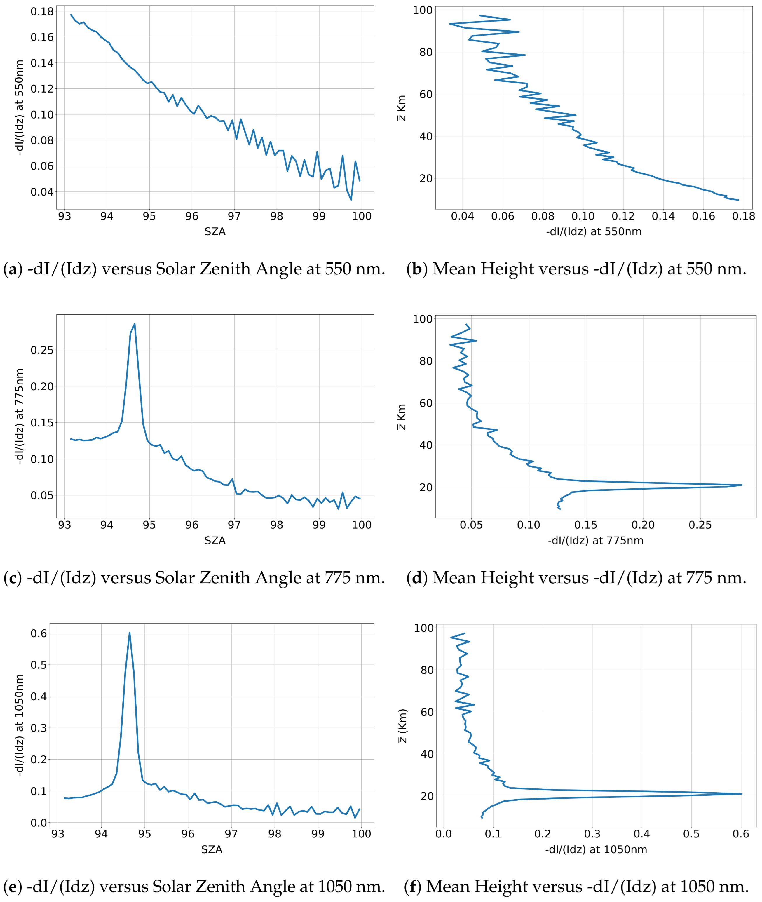
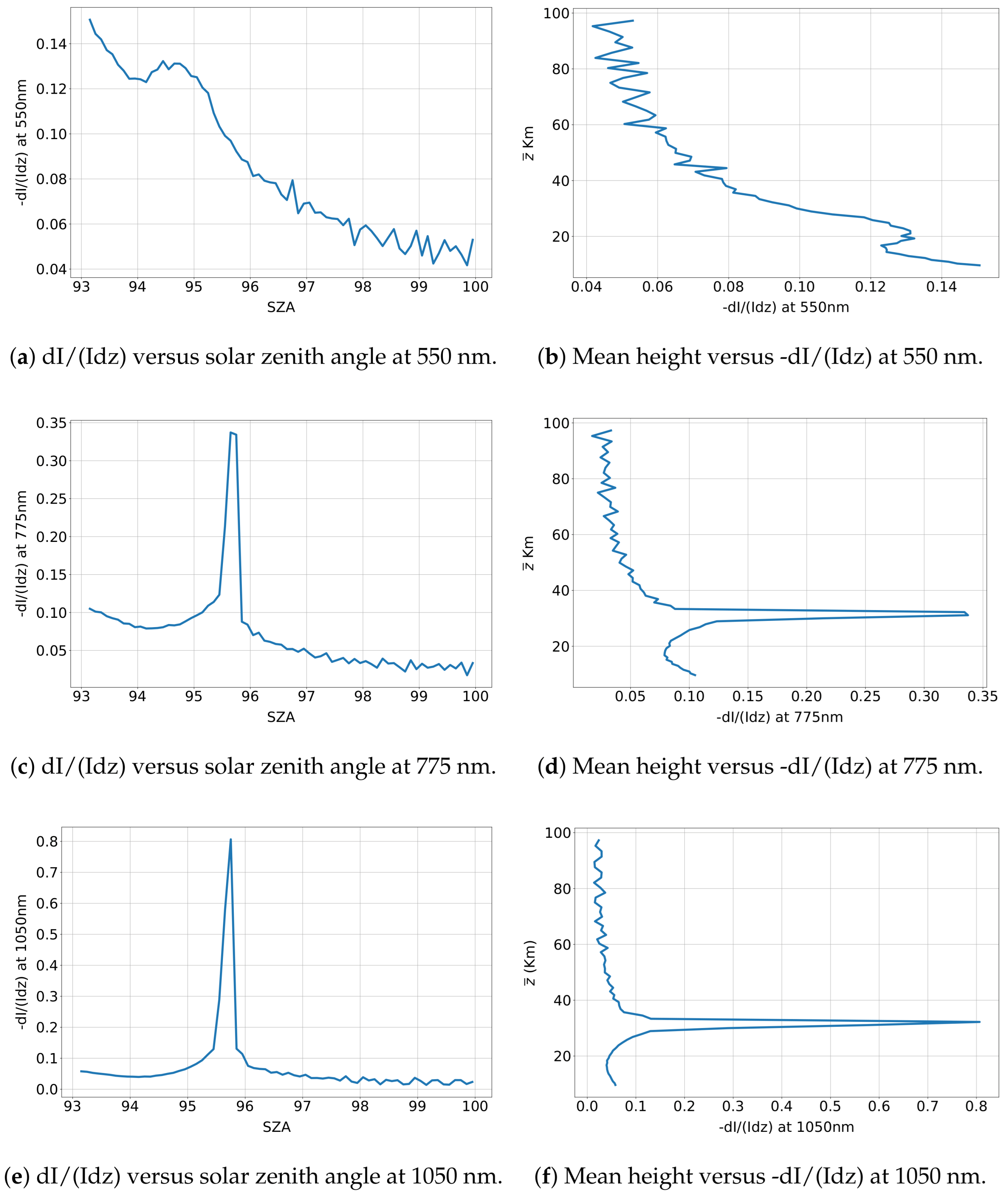
Figure 1. Schematic representation of daylight (SZA < 90°) and twilight (SZA > 90°) geometries with aerosol and ozone layer.
Remotesensing 17 02071 g001
Figure 2. Profiles of background aerosol, aerosol with Rayleigh, and aerosol with Rayleigh and ozone, with an AOD of 0.005 at 550 nm.
Remotesensing 17 02071 g002
Figure 3. Similar to Figure 2: aerosol profiles with Gaussian peaks at (a) 20 km and (b) 30 km.
Remotesensing 17 02071 g003
Figure 4. Comparison between the ratios I / I M C 400 as obtained from Hulbert’s sunset analytical model (in blue) [33] and Monte Carlo radiance (in green) both with and without ozone [24].
Remotesensing 17 02071 g004
Figure 5. Comparison between pseudospherical DISORT (in black) and Monte Carlo (in magenta) simulations at SZAs 85 ° , 90 ° , and 94 ° .
Remotesensing 17 02071 g005
Figure 6. Comparison of twilight radiance using (a) Monte Carlo model simulations and (b) ResPan-48 observations as a function of solar zenith angles (SZAs).
Remotesensing 17 02071 g006
Figure 7. Ratio of I 775 and I 450 vs difference of I 775 and I 760 at SZA = 85° using libRadtran’s DISORT simulations. The circles indicate ALH = 20 km, and triangles indicate ALH = 30 km with increasing AODs.
Remotesensing 17 02071 g007
Figure 8. Comparison of ResPan-48 measurements with (a) AERONET and (b) MERRA-2. The reference date are 12th December 2023 (indicated in red). Cases with poor agreement at SZA = 52.3° and 78.6° are highlighted with black circles.
Remotesensing 17 02071 g008
Figure 9. AOD retrieval using ResPan-48 measurements and the DISORT model in libRadtran when SZA = 65.2 and ozone = 330DU: (a) residual radiances from the difference between model and observations and (b) fitted model spectrum to observations in the 500–650 nm range, with AOD = 0.033.
Remotesensing 17 02071 g009
Figure 10. ResPan-48 radiance measurement at 821 nm on 21 March 2024 in Greenbelt, MD. The two SZAs (52.3 and 78.6) encircled in black indicate temporal scatter in the radiance plot.
Remotesensing 17 02071 g010
Figure 11. Ratios of I 775 and I 450 vs differences of I 775 and I 760 at SZA = 94° using Monte Carlo simulations. The notations of Figure 11 are similar to Figure 7.
Remotesensing 17 02071 g011
Figure 12. Modeled irradiance spectra for different aerosol optical depths (AODs) at an altitude of 30 km using Monte Carlo simulations.
Remotesensing 17 02071 g012
Figure 13. Illustrations of the aerosol peak at 20 km with an AOD of 0.005 at 550 nm obtained using Monte Carlo simulations.
Remotesensing 17 02071 g013
Figure 14. Illustrations of the aerosol peak at 30 km with an AOD of 0.005 at 550 nm obtained using Monte Carlo simulations.
Remotesensing 17 02071 g014
Figure 15. Comparison of ResPan-43 afternoon (red) and morning (blue) radiance measurement from Lauder, New Zealand.
Remotesensing 17 02071 g015
Figure 16. ResPan-43 observation at 775 nm used to estimate the aerosol layer height (ALH) using two methods: (a) the color ratio method, showing observational data compared against a model at 25 km ALH, and (b) the derivative method, detecting ALH both with and without refraction effects. Different days/twilights are shown in different colors in panel A. The twilight in red shown in panel A has been further analyzed in panel B using the derivative method.
Remotesensing 17 02071 g016
Figure 17. Vertical distribution of the aerosol backscatter ratio at 532 nm (BSR532) observed over Lauder on November 25, 2022. The horizontal dotted line indicates the tropopause.
Remotesensing 17 02071 g017
Figure 18. Twilight photometer measurement from (a) Brea, CA, and JPL data from (b,c) Table Mountain, CA, recorded on 25 June 2024.
Remotesensing 17 02071 g018
Figure 19. Comparison of modeled irradiance with different surfaces using DISORT simulation in libRadtran.
Remotesensing 17 02071 g019
Figure 20. Background aerosol detection by derivative method: (a) mean height versus -dI/(Idz) at 1050 nm with background aerosols; (b) -dI/(Idz) versus solar zenith angle at 1050 nm with background aerosols.
Remotesensing 17 02071 g020
Figure 21. MPLNET data (a,b) and ResPan-48 measurement (c) from 16 September 2023, Greenbelt, MD.
Remotesensing 17 02071 g021
Figure 22. Camera images with crosshairs (a) before broken clouds appear, (b) during broken cloud cover, and (c) after clouds have passed. Captured on 16 September 2023 in Greenbelt, MD.
Remotesensing 17 02071 g022
Table 1. Comparison of aerosol peak prediction at different wavelengths, with AOD = 0.005 at 550 nm.
Aerosol Peak Height (km)TRM Height Prediction at Wavelengths (nm)
5507751050
5.0--5.5
10.0--11.0
15.0--17.42
20.0-21.0321.03
30.020.029.3430.30
40.032.039.8640.57
Disclaimer/Publisher’s Note: The statements, opinions and data contained in all publications are solely those of the individual author(s) and contributor(s) and not of MDPI and/or the editor(s). MDPI and/or the editor(s) disclaim responsibility for any injury to people or property resulting from any ideas, methods, instructions or products referred to in the content.

