LIO-GC: LiDAR Inertial Odometry with Adaptive Ground Constraints

Abstract

LiDAR-based simultaneous localization and mapping (SLAM) techniques are commonly applied in high-precision mapping and positioning for mobile platforms. However, the vertical resolution limitations of multi-beam spinning LiDAR sensors can significantly impair vertical estimation accuracy. This challenge is accentuated in scenarios involving fewer-line or cost-effective spinning LiDARs, where vertical features are sparse. To address this issue, we introduce LIO-GC, which effectively extracts ground features and integrates them into a factor graph to rectify vertical accuracy. Unlike conventional methods relying on geometric features for ground plane segmentation, our approach leverages a self-adaptive strategy that considers the uneven point cloud distribution and inconsistency due to ground fluctuations. By optimizing laser range factors, ground feature constraints, and loop closure factors using graph optimization frameworks, our method surpasses current approaches, demonstrating superior performance through evaluation on open-source and newly collected datasets.

1. Introduction

With the development of robotics and autonomous driving, ground robots are no longer limited to indoor or planar environments, but as they are still constrained to the ground, terrain fluctuations should be taken into consideration.Traditional LiDAR SLAM methods primarily rely on point cloud registration and alignment [1,2] for localization and mapping, and their accuracy is significantly affected by the LiDAR scanning approach as well as the strategies used for feature extraction and matching. For most spinning LiDARs, due to the platform’s method of movement and the mounting configuration of the sensor, ground scans are very sparse most of the time, making it difficult to extract ground features and easily resulting in drift along the Z-axis. Most LiDAR SLAM methods just ignore these non-trivial problems, including ground fluctuations and roll and pitch changes of robots [3,4]. This will result in the rapid accumulation of Z-axis errors on uneven terrain.

Recent advances in LiDAR-based SLAM have made significant progress in addressing various challenges in robotic navigation and mapping. The integration of inertial measurement units (IMUs) and the adoption of factor graph optimization frameworks have improved overall system robustness and accuracy. Additionally, the emergence of neural SLAM approaches has introduced new possibilities for dense mapping and enhanced scene understanding. However, these improvements have primarily focused on general SLAM performance rather than specifically addressing the unique challenges posed by terrain variations and vertical accuracy maintenance in outdoor environments.

Existing outdoor datasets, such as KITTI [5], M2DGR [6] and MulRan [7], are predominantly collected in urban settings characterized by relatively flat and predictable ground surfaces. While urban datasets are undoubtedly useful for standard applications, they fall short of capturing the intricate complexities and multifaceted challenges posed by environments with significant terrain variations—such as hilly or mountainous regions with steep inclines and declines.

To address these limitations, we introduce LIO-GC, which effectively extracts ground features and integrates them into a factor graph to rectify vertical accuracy. Unlike conventional methods relying on geometric features for ground plane segmentation, our approach leverages a self-adaptive strategy that considers uneven point cloud distribution and inconsistency due to ground fluctuations.

The main contributions of this paper are as follows.

1.

A SLAM framework named LIO-GC is proposed, which integrates the Cloth Simulation Filtering (CSF) algorithm to extract the ground points to significantly reduce Z-axis drift in mapping in diverse environments.

2.

Optimizations including the use of efficient data structures, parallel processing techniques, and adaptive resolution adjustments are introduced, enabling the algorithm to operate more efficiently in real-time applications.

3.

A newly collected dataset featuring environments with notable terrain undulations and various ground objects is developed for the comprehensive evaluation of SLAM algorithms.

The rest of this paper is organized as follows. Section 2 provides an overview of related works, including the evolution of traditional SLAM methods, modern approaches, and recent deep learning and neural SLAM. Section 3 presents our proposed LIO-GC method, including the system architecture, mathematical modeling, and algorithmic implementation. Section 4 shows the experiments and results, demonstrating the effectiveness of LIO-GC in reducing Z-axis drift and the efficiency of the optimized CSF [8] implementation. Section 5 provides some discussion of the results. Finally, we present brief conclusions regarding LIO-GC and perspectives that may be explored in future work.

2. Related Works

2.1. Traditional SLAM Methods

The development of LiDAR-based SLAM can be traced through several evolutionary phases, beginning with foundational geometric approaches [9]. Among early studies, LOAM [10] (LiDAR Odometry and Mapping) decomposed the complex simultaneous localization and mapping problem into two algorithms to achieve low drift and low computational complexity. One algorithm was responsible for high-frequency, low-precision motion estimation, while the other algorithm focused on low-frequency, high-precision point cloud matching and alignment. Although this dual approach achieved better localization and mapping performance, additional processing was still required to ensure acceptable accuracy.

Building upon LOAM’s foundations, IMLS-SLAM [11] emerged as another notable method, relying on a scan-to-model matching approach for odometry measurements. The model was represented by an IMLS (Implicit Moving Least Squares) surface descriptor based on past scan point clouds. Similar to LOAM in positioning, IMLS-SLAM attempted to improve mapping accuracy through sophisticated point cloud-processing techniques.

The progression towards ground-aware methodologies began with LeGO-LOAM [12], which demonstrated a lightweight design with optimization related to ground features. It used point cloud segmentation to eliminate noise and conduct feature extraction in order to capture distinctive plane and edge features. Subsequently, a two-step Levenberg–Marquardt optimization method was employed on the plane and edge features to address the different components of the 6-DoF transformation in consecutive scans.

2.2. Factor Graph-Based Approaches and Recent Developments

The introduction of probabilistic frameworks marked a significant advancement in SLAM methodology. Inspired by these works, LIO-SAM [13] was proposed, introducing the concept of a factor graph [14,15,16] into SLAM and integrating IMU pre-integration [17,18] and GPS factors into the back-end optimization module [19]. This approach leveraged the correlated relationships among multiple sensors to reduce cumulative errors [20] and employed an incremental factor graph pattern to enhance overall system accuracy and robustness [21]. The introduction of factor graphs also reduced the frequency of high-intensity computations, thereby lowering average computational resource utilization.

Contemporary traditional methods continued to evolve with specialized ground segmentation techniques. Recent advances in geometric-based approaches include Patchwork++ [22], Adaptive Patchwork [23], and LOG-LIO [24] which focused on fast and robust ground segmentation [25,26] for 3D point clouds. These methods addressed partial under-segmentation issues through adaptive partitioning and spatial–temporal context analysis.

2.3. Deep Learning and Neural SLAM

The emergence of deep learning-based SLAM methods has introduced revolutionary paradigms for visual and geometric understanding [27]. The neural SLAM revolution began with dense visual approaches and has recently expanded to incorporate advanced neural representations.

An early pioneer in integrating learning-based approaches with LiDAR SLAM was SuMa++ [28], which introduced efficient LiDAR-based semantic SLAM capabilities. This method combined traditional geometric SLAM with semantic segmentation networks to provide enhanced scene understanding and mapping consistency. SuMa++ leveraged deep learning for semantic labeling of point clouds while maintaining efficient surfel-based map representations. The integration of semantic information enabled more robust loop closure detection and improved mapping accuracy through semantic consistency checks. However, despite its semantic awareness capabilities, SuMa++ still faced challenges in handling significant terrain variations and maintaining vertical accuracy in undulating environments, as its semantic segmentation focused primarily on object-level understanding rather than detailed ground geometry variations.

Gaussian Splatting SLAM [29] leverages neural representations for dense mapping applications with improved computational efficiency. This work demonstrated the potential of integrating modern machine learning techniques with traditional SLAM frameworks, showcasing enhanced performance in complex visual environments. Similarly, GS-SLAM [30] focuses on dense visual SLAM applications using 3D Gaussian splatting methodologies. Their approach represented a significant advancement in neural rendering techniques applied to real-time SLAM applications.

The field has also witnessed advances in loop closure detection and neural mapping approaches. Loopy-SLAM [31] is a dense neural SLAM method that effectively addresses loop closure challenges in complex environments, demonstrating improved robustness in long-term navigation scenarios. These neural approaches complement traditional geometric methods by providing enhanced feature representation and matching capabilities.

3. Method

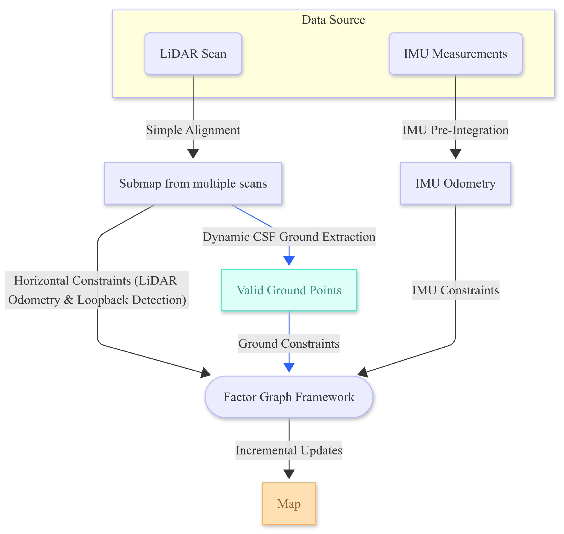
3.1. Overview

The proposed LIO-GC (LiDAR-Inertial Odometry with Ground Constraints) method is designed to address the challenge of Z-axis drift in LiDAR-Inertial Odometry (LIO) systems, particularly on undulating terrain. This is achieved by integrating optimized ground constraints derived from Cloth Simulation Filtering (CSF) [8,32] into the LIO-SAM framework. The overall architecture of LIO-GC is illustrated in Figure 1 and consists of the following key components.

1.

LiDAR and IMU Data Preprocessing: raw LiDAR point clouds and IMU data are preprocessed to remove noise and outliers.

2.

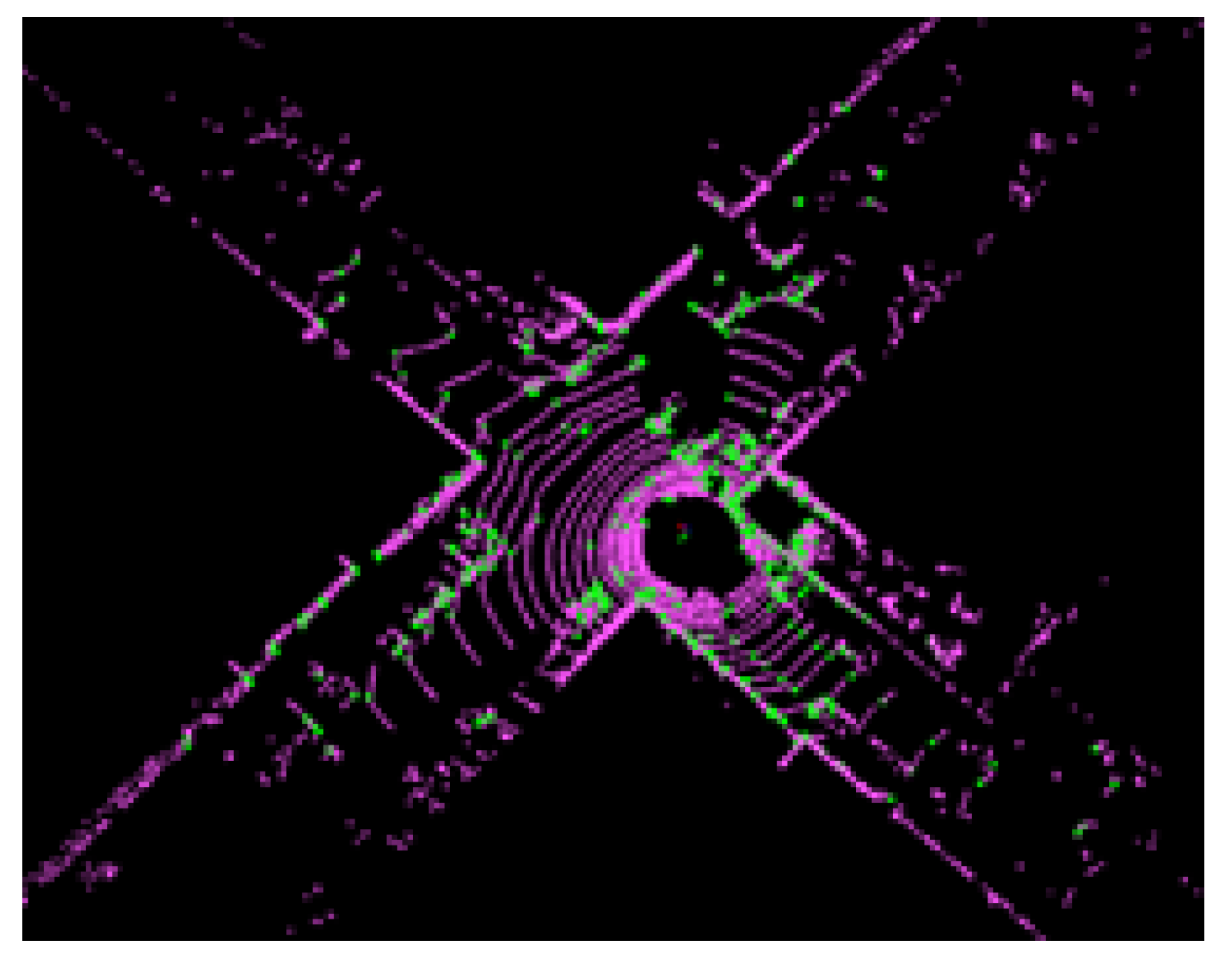
Optimized Cloth Simulation Filtering (CSF): ground points are extracted from the LiDAR point cloud using an optimized CSF algorithm.

3.

Ground Constraint Factor Integration: the extracted ground points are used to create ground features, which are integrated into the LIO-SAM factor graph for ground constraints.

4.

Factor Graph Optimization: the LIO-SAM framework optimizes the system’s state estimation using the factor graph, incorporating the ground constraint factor to reduce Z-axis drift between factor nodes.

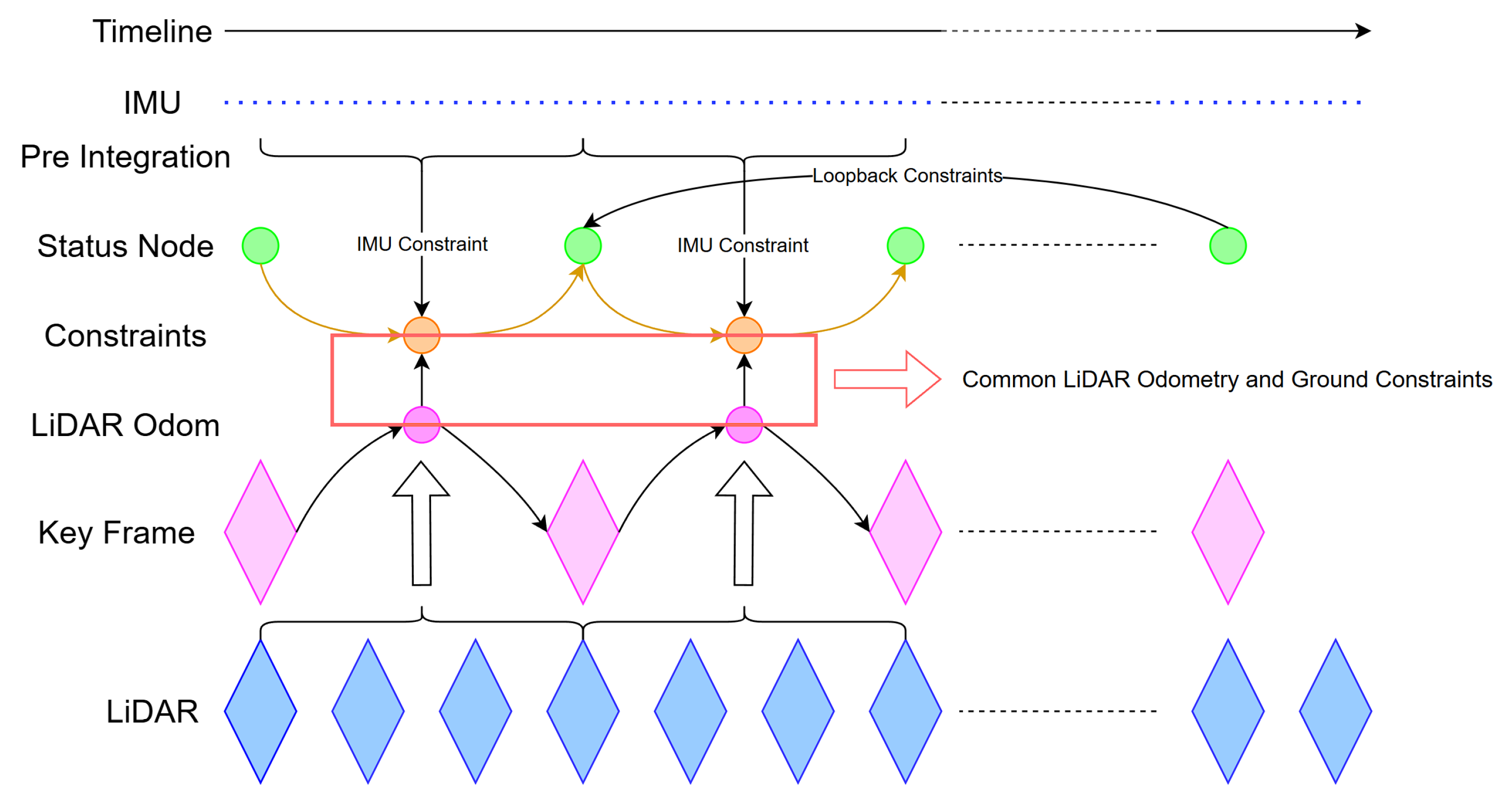
3.2. Dual Pipelines for Horizontal and Ground Constraints

Due to LiDAR scanning type and the operating trajectory of the platform, the point clouds obtained typically contain very limited vertical features. Hence, extracting ground features from the data meant for basic feature extraction is not appropriate. We have designated the horizontal constraint and ground constraint processes as two distinct pipelines. The horizontal constraint pipeline is derived from LIO-SAM, leveraging co-planar geometric relationships while addressing lower confidence in Z-axis predictions. In contrast, the ground constraint pipeline primarily enforces height restrictions during back-end optimization, though it demonstrates reduced reliability in the horizontal direction.

In the ground constraint pipeline, suppose that $p_t$ is a point on a laser scan line. The smoothness of $p_t$ can be represented by the following formula:

$$c={\displaystyle \frac{1}{\left|n\right|·p_{(r,i)}}}∥\sum _{j\in n,j\ne i}\left[p_{(r,i)}-p_{(r,j)}\right]∥$$

(1)

where c is the smoothness of $p_i$, and n represents the set of adjacent points in the r-th scan frame centering on $p_i$. $p_j$ is another point in n other than $p_i$. When extracting features from point clouds, it is essential to remove features that are prone to disappearing or becoming isolated.

The extraction of edge and surface features from point clouds is illustrated in Figure 2, with surface features highlighted in magenta and edge features marked in green. The correspondence between features enables self-motion estimation over a short period of time, which is then used to construct a submap within several frames. Similar to LIO-SAM, a keyframe selection concept is adopted in LIO-GC for scan matching and pose estimation as a preliminary LiDAR odometry factor.

Due to the limited computational resources and the need for timeliness, here, we introduce a dynamic CSF ground extraction method. In the initial setup, we use a small number of point cloud frames (five frames) to form a single submap. Considering the complexity of environmental complexity, a high frequency of ground extraction through CSF may not necessarily result in higher accuracy. Therefore, we ensure an adequate number of ground points in the submap before conducting CSF extraction, and this quantity is dynamic, changing with the complexity of height variations in the estimated trajectory. In other words, submaps from estimated poses within a certain distance will be considered for ground feature extraction.

Inspired by the concept of region of interest (ROI), during CSF, only the part that falls onto the ground points is retained in preparation for subsequent matching tasks. For the odometry measurement, these ground features serve as constraint factors to optimize the Z-axis drift, roll, and pitch and further back-end optimization.

3.3. Back-End Optimization with Separate Ground and Horizontal Constraints

Back-end optimization is a critical component of LiDAR-Inertial Odometry (LIO) systems, where it serves to refine and improve the accuracy of the estimated trajectory. Like LIO-SAM, the back-end optimization is framed within a factor graph optimization framework. In this graph, nodes represent the vehicle’s poses at various time steps, while edges encode the constraints derived from homogeneous or heterogeneous sensor measurements, such as those from the inertial measurement unit (IMU) and LiDAR. The objective of back-end optimization is to minimize a cost function that incorporates the residuals from these sensor measurements, thereby adjusting the poses to achieve the best possible alignment with the observed data. Standard optimization methods, like Gauss–Newton or Levenberg–Marquardt [33], are used to iteratively solve the nonlinear least squares problem. These methods work to reduce drift and errors, ensuring that the trajectory estimate becomes more accurate over time. Factors such as odometry from the IMU and LIDAR scans contribute to the cost function, helping to correct pose estimates by aligning them with the observed measurements.

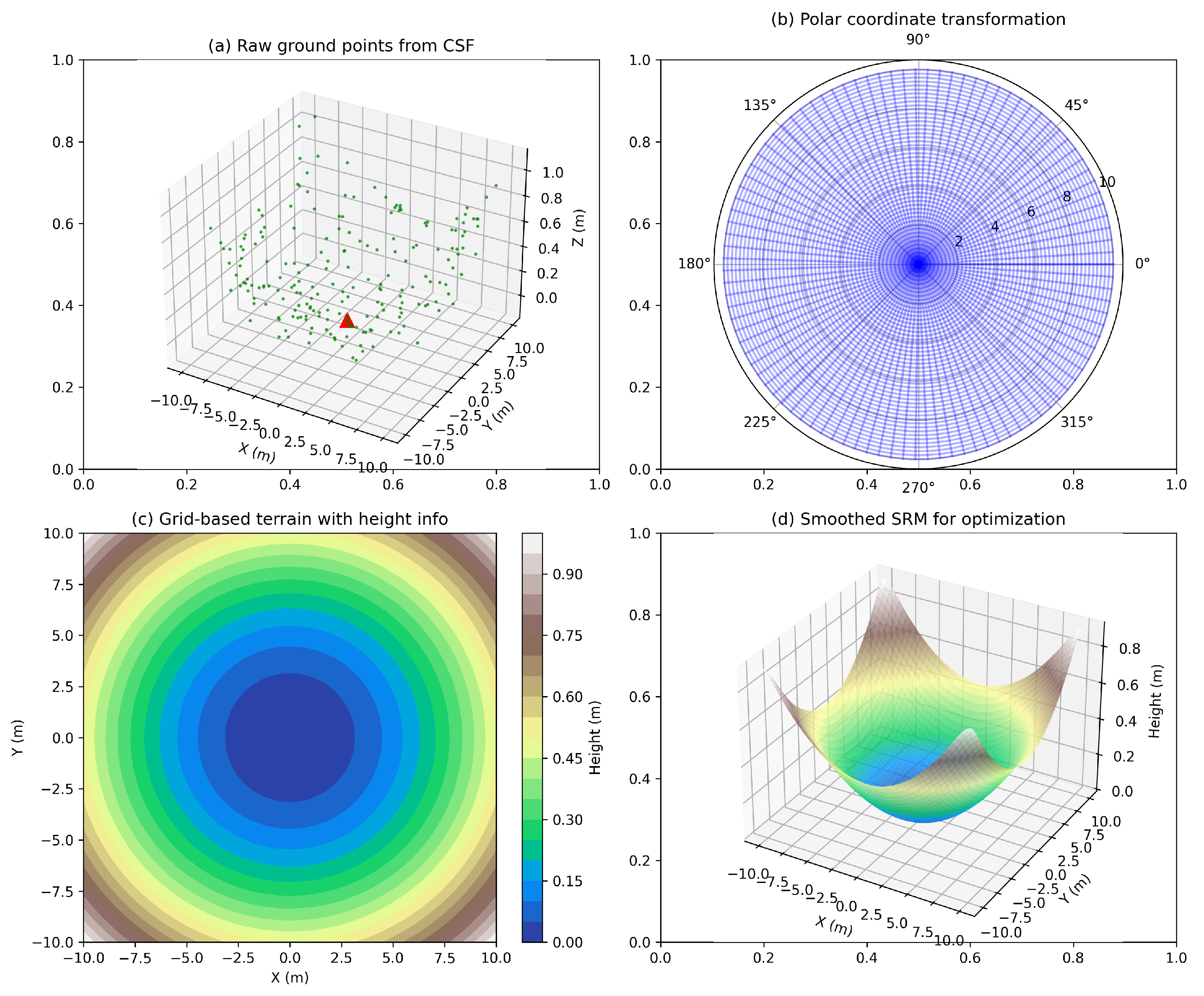
3.3.1. Slope Range Map

The cloth feature fitting the ground is not suitable for alignement with the other because there are too many particles and edges. Inspired by scan context [34], we introduce a vertical loopback constraint derived from the range map model. Each grid in this map provides not only the height but also the smoothed slope and direction of the ground relative to the current keyframe position.

The slope range map (SRM) is a grid-based representation of the terrain surrounding the vehicle, generated from CSF (Cloth Simulating Filtering) ground features. This map uses polar coordinates to model the terrain, providing essential information about the slope and direction of the ground relative to the vehicle’s current position. To ensure smooth and stable terrain modeling, the grid data in the range map is smoothed before it is used for back-end optimization. This helps to reduce noise from sensor data and ensures that terrain features such as slopes and directions are represented as continuous gradients rather than abrupt noisy variations.

1.

Height $h(r,\theta )$: the elevation of the terrain at a distance (radius) r and direction (angle) $\theta$ relative to the vehicle’s current position.

2.

Slope $\alpha (r,\theta )$: the angle of the terrain’s incline relative to the horizontal plane at the given point. The slope is defined as the change in height per unit distance in the radial direction.

3.

Direction $\varphi (r,\theta )$: the orientation of the slope relative to the vehicle’s current heading, which indicates the steepest descent at that particular point.

As illustrated in Figure 3, the SRM construction process involves four sequential steps to transform raw ground points into structured terrain constraints. Initially, ground points extracted through CSF are organized into a polar coordinate system centered at the vehicle’s current position (Figure 3a). These points are subsequently binned into a polar grid structure, where each cell $(r,\theta )$ represents a specific radial distance and angular direction relative to the vehicle (Figure 3b). The discretized terrain data are then processed to compute height $h(r,\theta )$, slope $\alpha (r,\theta )$, and direction $\varphi (r,\theta )$ for each grid cell (Figure 3c). Finally, Gaussian smoothing is applied to create continuous terrain representations that effectively encode local topographic features for integration into factor graph optimization (Figure 3d).

The smoothing process involves applying a Gaussian filter technique to the height and slope data in the polar grid. The main goal is to smooth both the radial and angular variations of the terrain. The Gaussian smoothing function can be defined as follows:

$$\widehat{h}(r,\theta )=\sum _{r^{\prime },{\theta }^{\prime }}G(r-r^{\prime },\theta -{\theta }^{\prime })·h(r^{\prime },{\theta }^{\prime })$$

(2)

where $\widehat{h}(r,\theta )$ is the smoothed height value at grid point $(r,\theta )$, $h(r^{\prime },{\theta }^{\prime })$ is the original height value at neighboring grid points, and $G(r-r^{\prime },\theta -{\theta }^{\prime })$ is the Gaussian kernel applied to the surrounding points, defined as

$$G(r-r^{\prime },\theta -{\theta }^{\prime })={\displaystyle \frac{1}{2\pi {\sigma }^2}}\exp \left(-{\displaystyle \frac{{(r-r^{\prime })}^2+{(\theta -{\theta }^{\prime })}^2}{2{\sigma }^2}}\right)$$

(3)

where $\sigma$ controls the smoothing scale, determining the size of the neighborhood over which the smoothing is applied.

After smoothing, each point $(r,\theta )$ in the range map contains the corresponding height and terrain slope.

In back-end optimization, the slope range map helps correct the roll and pitch estimates by integrating terrain-induced constraints at a lower frequency and reduces Z-axis drift in continuous time. The vertical loopback constraint uses the slope and direction data to adjust the vehicle’s pose in regions with undulating terrain. This constraint improves accuracy in environments where traditional methods often fail to handle roll and pitch correctly.

The slope range map influences the cost function in the optimization process. The cost function is typically defined as a sum of squared errors between predicted and observed sensor data. The slope range map adds a term to the cost function that penalizes deviations in roll and pitch based on the predicted terrain features. This allows the optimization algorithm to prioritize the correction of these angles while maintaining consistency with the surrounding terrain.

The error function can be defined as

$$E_{\mathrm{roll},\mathrm{pitch}}=\sum _{r,\theta }{\left|\widehat{\alpha }(r,\theta )-{\widehat{\alpha }}_{\mathrm{observed}}(r,\theta )\right|}^2+{\left|\widehat{\varphi }(r,\theta )-{\widehat{\varphi }}_{\mathrm{observed}}(r,\theta )\right|}^2$$

(4)

where $\widehat{\alpha }(r,\theta )$ is the predicted slope from the map; $\widehat{\varphi }(r,\theta )$ is the predicted direction; and ${\widehat{\alpha }}_{observed}(r,\theta )$ and ${\widehat{\varphi }}_{observed}(r,\theta )$ are the measured slope and direction from the sensor.

After integrating the terrain-based constraints, the back-end optimization algorithm adjusts the vehicle’s pose (position and orientation) to match both the observed sensor data and the terrain features encoded in the slope range map. This refinement process ensures that the vehicle’s trajectory accounts for the dynamic terrain without over-penalizing slight roll and pitch variations in flat areas.

3.3.2. Factor Graph Optimization Incorporating Ground Constraints

This section introduces the factor graph optimization model based on ground constraint along with the mentioned constraints. In order to effectively integrate LiDAR odometry, IMU pre-integration, ground constraints, and loop detection, we abstract the fusion of sensors using a factor graph model as a nonlinear optimization problem [35]. Traditional filtering-based sensor fusion methods, such as Kalman filtering [36] and its nonlinear extensions like EKF [37,38], face challenges in establishing correlations in high-dimensional data spaces. The primary advantage of the factor graph is its ability to re-linearize and iterate, which allows for iterative optimization to bring the optimized state closer to the optimal. The fundamental idea behind factor graph optimization considering ground constraints is to associate the system’s state over a period of time (including the mobile platform state and keyframes) with observation data (e.g., LiDAR scan and IMU data flow) to construct a graphical model. Global optimization is achieved based on Bayes’ theorem [39].

For any system state and observations at a given time period, the factor graph model enables the calculation of the maximum a posteriori probability of the joint distribution probability density for all random variables, as shown below.

$$X^{\mathrm{MAP}}=\arg \underset{X}{\max }\left(p\left(X|Z\right)\right)=\arg \underset{X}{\max }\prod _i{\varphi }_i\left(x_i\right)$$

(5)

where $X^{MAP}$ represents the maximum posterior probability estimate of the state to be estimated, X represents the unknown state variable in the current factor graph model, p represents the joint probability distribution function in the current factor graph model, $\varphi$ is a factor node, and x is a variable node. This section combines the factor graph optimization method with ground constraints, describing the SLAM problem as factor nodes and variable nodes in the factor graph model, thus achieving global optimization based on factor graph inference. $X_k$ is defined as below:

$$X_k={\left[{\left(R_B^W\right)}^T,{\left(p_B^W\right)}^T,{\left(v_B^W\right)}^T,b_g^T,b_a^T\right]}^T$$

(6)

Optimizing by directly using state variables of location information, rather than their errors, provides greater flexibility, can simplify computations, and often results in more accurate and robust location estimates [40], especially in complex or dynamic environments. This approach is particularly advantageous when the system needs to adapt to changing conditions or incorporate additional state components.

To ensure algorithm stability, we opted for incremental smoothing rather than offline maximum likelihood estimation in our work. This approach allows the system to promptly constrain range errors during real-time operation of the SLAM system, preventing the risk of becoming stuck in local optima during subsequent optimizations. We also introduced a sliding window approach to maintain the real-time performance of the entire system while ensuring accuracy in localization and mapping. The sliding window maintains a fixed-length buffer of recent keyframes, denoted $\mathcal{W}=\{x_{k-n},x_{k-n+1},\dots ,x_k\}$, where n represents the window size and $x_k$ is the most recent keyframe pose. When a new keyframe is generated by the main framework, the system performs the following operations.

1.

Local Bundle Adjustment: For all keyframes within a certain spatial distance threshold $d_{thresh}$ from the new keyframe, odometry measurements are computed, and bundle adjustment is performed within the current sliding window:

$$\min \sum _{i\in \mathcal{W}}{\parallel f(x_{i-1},p_{DR-odom,i-1},p_{ground,i-1},p_{imuPre,i-1})-x_i\parallel }_{{\Omega }_{i-1}}^2$$

(7)

2.

Window Management: When the window size exceeds the predefined limit, the oldest keyframe $x_{k-n-1}$ is marginalized out, and its information is compressed into prior factors to maintain computational efficiency.

3.

Loop Closure Handling: Upon loop closure detection between the current pose $x_i$ and a historical pose $x_{k+1}$ (where the historical pose may be outside the current window), the system extends the optimization scope to include both poses:

$$\begin{array}{c}\min \sum _{i\in \mathcal{W}\cup \{k+1\}}{∥f(x_{i-1},p_{DR-odom,i-1},p_{ground,i-1},p_{imuPre,i-1})-x_i∥}_{{\Omega }_{i-1}}^2\hspace{1em}\hspace{1em}\hspace{1em}\hspace{1em} \hfill \\ \hfill +{∥g(x_i,l_{i,k+1})-x_{k+1}∥}_{{\theta }_{i,k+1}}^2\end{array}$$

(8)

Following loop closure, a global bundle adjustment is performed on all keyframes to propagate the correction throughout the entire trajectory.

As shown in Figure 4, two adjacent poses $x_i$ and $x_{i-1}$ are connected by the LiDAR odometry factor p, the ground constraint factor, and the IMU preintegration factor. The relationship between these two adjacent pose nodes and their conditional probability model can be represented as

Figure 4. Overview of the factor graph processing framework shown with time flow.

Figure 4. Overview of the factor graph processing framework shown with time flow.

$$x_i=f(x_{i-1},p_{DR-odom,i-1},p_{ground,i-1},p_{imuPre,i-1})+{\omega }_i$$

(9)

where $x_i$ refers to the robot pose state at time i; $p_{DR-odom,i-1}$ refers to the LiDAR odometry factor between consecutive poses $x_{i-1}$ and $x_i$; $p_{ground,i-1}$ refers to ground constraint factor derived from CSF-extracted ground features; $p_{imuPre,i-1}$ refers to IMU preintegration factor incorporating inertial measurements; and ${\omega }_i$ refers to the zero-mean Gaussian noise vector.

$$\begin{array}{cc}\hfill & P\left(x_i\mid x_{i-1},p_{DR-odom,i-1},p_{ground,i-1},p_{imuPre,i-1}\right)\hfill \\ \hfill & =N\left(f\right(x_{i-1},p_{DR-odom,i-1},p_{ground,i-1},p_{imuPre,i-1},{\Omega }_{i-1})\hfill \end{array}$$

(10)

where ${\Omega }_{i-1}$ represents zero-mean Gaussian [41] additive noise ${\omega }_i$. When a loop detection factor is generated, it means that the current position bears enough similarity to a past visited location to create a constraint. The following formulas express the relationship between the loop constraint $l_{i,k+1}$ and the pose of mobile platform $x_i$, $x_{k+1}$. $l_{i,k+1}$ represents the pose change relationship between the current observation of the mobile platform at $x_i$ and the corresponding submap of $x_{k+1}$.

$$x_{k+1}=g\left(x_i,l_{i,k+1}\right)+{\beta }_{i,k+1}$$

(11)

$$P\left(x_{k+1}\mid x_i,l_{i,k+1}\right)=N\left(g\left(x_i,l_{i,k+1}\right),{\theta }_{i,k+1}\right)$$

(12)

where ${\theta }_{i,k+1}$ is the covariance corresponding to the Gaussian noise ${\beta }_{i,k+1}$. The Equation (13) integrates all mobile platform pose nodes and their corresponding constraints:

$$U=\left\{\begin{array}{c}{p}_{DR-odom,i},p_{ground,i},p_{imuPre,i},l_{i,k+1}\end{array}\right\}$$

(13)

The posterior probability within a certain sliding window can be expressed as

$$P\left(X|U\right)\propto \prod P\left(x_i|x_{i-1},p_{DR-odom,i-1},p_{ground,i-1},p_{imuPre,i-1}\right)\prod P\left(x_{k+1}\mid x_i,l_{i,k+1}\right)$$

(14)

By maximizing the left-hand side of the above equation, we can incrementally solve this maximum a posteriori probability problem through iSAM2 [14], a smooth mapping model, with the following equation:

$$\begin{array}{cc}\hfill X^{\mathrm{MAP}}& =\underset{X}{\arg \max }\left(P\left(X|U\right)\right)\hfill \\ \hfill & =\arg \underset{X}{\min }\left(-\log \left(P\left(X\mid U\right)\right)\right)\hfill \\ \hfill & =\underset{X}{\arg \min }(\sum _i{\parallel f\left(x_{i-1},p_{DR-odom,i-1},p_{ground,i-1},p_{imuPre,i-1}\right)-x_i\parallel }_{{\Omega }_{i-1}}^2\hfill \\ \hfill & +\sum _i{∥g\left(x_i,l_{i,k+1}\right)-x_{k+1}∥}_{{\theta }_{ij}}^2)\hfill \end{array}$$

(15)

4. Experiments and Results

4.1. Dataset Description

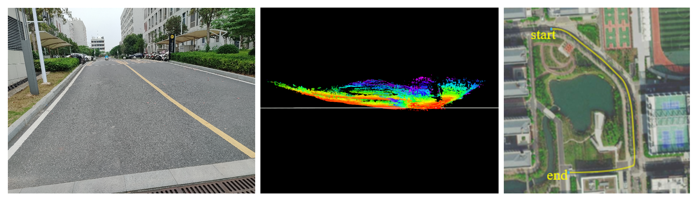
• “Path” Datasets: Our newly collected dataset, named “Path”, was compiled to capture different environmental characteristics and terrains to comprehensively evaluate the performance of SLAM algorithms including the proposed LIO-GC. As shown in Figure 5, this dataset features substantial ground undulations and includes complex environmental objects such as lakes, dirt mounds, trenches, and irregular buildings. The platform does not revisit any previous locations in a trajectory. Therefore, no loop closure should occur in SLAM algorithms.

  Figure 5. Features of our dataset: pictures of slopes (left), ground points generated by LIO-GC with horizontal viewport (middle), and satellite pictures (right).

  Figure 5. Features of our dataset: pictures of slopes (left), ground points generated by LIO-GC with horizontal viewport (middle), and satellite pictures (right).
• S3E Dataset: This is a large-scale multi-robot multimodal dataset [42] designed for collaborative SLAM research, featuring diverse environments and cooperative trajectory patterns, making it suitable for evaluating SLAM algorithms in various scenarios. This dataset was made using a fleet of unmanned ground vehicles, each equipped with a 16-line LiDAR, several high-resolution cameras, a 9-axis IMU, and a dual-antenna RTK receiver. Here, we use the “Dormitory” subset as our additional testing data because this part has complete ground truth.

Our “Path” dataset is gathered by a wheeled mobile platform equipped with a single board computer (SBC). The machine is small and lightweight and has the capability to operate normally within the range of 9 V to 24 V, which made it easy to fit the mobile sensor platform with a 16-line LiDAR, an IMU, and an RTK module. The hardware setup is as shown in Figure 6. The sensors are calibrated in advance.

To assess the performance and robustness of our algorithm in real-world scenarios, we designed an experimental plan. Algorithms were tested with our “Path” dataset to assess the performance and robustness in real-world scenarios. In addition, the S3E dataset was used to benchmark the proposed LIO-GC under relatively common environmental conditions, where the ground is mostly flat.

4.2. Evaluation Metrics

The performance of the proposed LIO-GC and other algorithms was evaluated using the following metrics.

• Root Mean Square Error (RMSE): This metric measures the average magnitude of the error in the estimated trajectory. It provides a quantitative assessment of the system’s localization accuracy.
• Maximum Error (Max Error): This metric measures the maximum error during the whole experiment process. It provides an indication of the worst-case performance of the system, like running on a long path without any loopback.
• Computational Efficiency: This metric measures the computational resources required by the system, including average CPU and memory consumption. It provides an assessment of the system’s real-time performance and the possibility of integration with other systems

4.3. Overall Performance Comparison

Here, we tested the performance of our algorithm and others on the S3E dataset and our “Path” dataset. The test on the S3E dataset was carried out by selecting a robot within an environment and applying the candidate algorithms. The trajectory of each robot was evaluated by comparing it with the reference ground truth for assessment. The test on our “Path” dataset emulated real targeted scenarios.

As shown in Figure 7, the positioning trajectories of LIO-GC and LIO-SAM were compared by X, Y, and Z-axis on “Path”. From the Z-axis records, our algorithm showed much better vertical accuracy, with a 63.2% reduction in RMSE compared to LIO-SAM (0.14 m vs. 0.38 m).

It can be observed that LIO-SAM achieved high accuracy in the horizontal direction, yet significant errors persisted in vertical accuracy. The proposed LIO-GC effectively enhanced the overall accuracy of Z-axis positioning, closely approximating the ground truth of the Z-axis with 64.7% improvement in mean error (0.12 m vs. 0.34 m) and 3.2% reduction in maximum error (8.49 m vs. 8.77 m).

Figure 8 illustrates the variation in APE (absolute pose error) over time for the two algorithms on “Path”. The errors of LIO-GC and LIO-SAM were relatively close to each other. However, as the operation continued, the error of LIO-GC quickly converged to a lower level with smaller fluctuations, maintaining an average error below 0.2 m after the 200 s mark, while LIO-SAM exhibited more pronounced oscillations, with peak errors reaching up to 1.0 m. Figure 9 presents the error statistical analysis of the two algorithms.

Table 1. Results of algorithms on “Path”.

Algorithm	RMSE (m)	Mean (m)	SSE (m2)	Max (m)
LIO-SAM	0.38	0.34	176.98	8.77
Faster-LIO [43]	0.36	0.30	188.56	11.08
Point-LIO [44]	0.76	0.69	293.31	11.96
r3live [45]	Failed	Failed	Failed	Failed
LIO-GC (ours)	0.14	0.12	171.46	8.49

summarizes the comparative results of the proposed LIO-GC method in this paper and other methods for the “Path” data.

In the comparative experiments conducted in basically flat environments, our algorithm demonstrated that it did not perform worse than the original LIO-SAM. The comparative results of Z-axis and evaluation metrics on S3E’s “Dormitory” dataset are shown in Figure 10 and

Table 2. Results of algorithms on S3E’s “Dormitory”.

Algorithm	RMSE (m)	Mean (m)	SSE (m2)	Max (m)
LIO-SAM	4.43	3.99	93,588.16	13.92
Faster-LIO	10.24	7.21	1,856,489.33	25.50
Point-LIO	7.31	5.97	938,152.02	30.58
r3live	8.64	7.14	1,324,997.26	31.07
LIO-GC (ours)	4.46	4.12	72,086.44	10.43

.

During the experiment, we recorded CPU usage at a frequency of one sample per second. The resource consumption of the algorithm optimized with SRM was significantly reduced, although it still used a substantial amount of resources during the system’s initial startup phase.

Table 3. Statistics on CPU usage.

Algorithm	Max (%)	Average (%)
LIO-GC (without SRM)	100.0	88.7
LIO-GC (with SRM)	99.2	64.4

shows our statistics of CPU utilization throughout the experiment.

4.4. Ablation Study

To validate the individual contributions of each component in LIO-GC, we conducted comprehensive ablation studies on both the “Path” and “Dormitory” datasets.

Table 4. Ablation study results on the “Path” dataset.

Configuration	RMSE (m)	Mean (m)	Max (m)	CPU (%)
LIO-SAM (baseline)	0.38	0.34	8.77	45.2
LIO-GC (CSF only)	0.32	0.29	6.84	88.7
LIO-GC (no optim.)	0.26	0.24	6.12	85.3
LIO-GC (complete)	0.14	0.12	8.49	68.2

and

Table 5. Ablation study results on the “Dormitory” dataset.

Configuration	RMSE (m)	Mean (m)	Max (m)	CPU (%)
LIO-SAM (baseline)	0.89	0.76	15.43	43.8
LIO-GC (CSF only)	0.54	0.48	14.67	86.2
LIO-GC (no optim.)	0.31	0.28	9.45	83.7
LIO-GC (complete)	0.29	0.26	9.82	62.1

present the results of different system configurations. Here, the “CPU” refers to average consumption.

The ablation study revealed the progressive improvements achieved by each component of LIO-GC. On the “Path” dataset, the introduction of CSF filtering reduced RMSE by 15.8% (from 0.38 m to 0.32 m) compared to the baseline LIO-SAM, while the complete LIO-GC system achieved a substantial 63.2% RMSE reduction (from 0.38 m to 0.14 m). Similarly, on the “Dormitory” dataset, CSF integration provided a 39.3% improvement, and the full system delivered a 67.4% enhancement in localization accuracy.

The computational efficiency optimizations successfully addressed the performance bottleneck introduced by ground constraint processing. While CSF integration nearly doubled CPU usage (from 44% to 87%), the optimized LIO-GC reduced this overhead significantly, maintaining CPU usage at 68.2% and 62.1% on the respective datasets—a reduction of approximately 23–25% compared to the unoptimized version—while preserving superior accuracy performance.

These results demonstrate that LIO-GC effectively balances computational efficiency with localization precision, achieving substantial accuracy improvements while maintaining real-time feasibility for practical deployment.

5. Discussion

5.1. Summary of Key Findings

The experimental results in Table 1 validate the effectiveness of the proposed LIO-GC framework in mitigating Z-axis drift while maintaining real-time performance. Performance on “Path” showed that the proposed LIO-GC outperforms LIO-SAM in z-axis precision under uneven environments. According to Table 2, LIO-GC maintains comparable accuracy to LIO-SAM in S3E’s “Dormitory” scenario, with even smaller maximum errors, showcasing superior stability.

Compared with LIO-SAM, the proposed CSF-integrated LIO-GC proposed in this paper reduces the max error by about 23% on “Path”, but at the cost of an approximately 48% increase in CPU load on i7-13700F (Intel Corporation, Santa Clara, CA, USA).

Given that our method’s optimization is primarily targeted towards LiDAR systems with fewer lines working in terrains with significant undulations, testing in relatively flat terrains (e.g., with S3E’s “Dormitory”) showed that our method reduced maximum error and indicated that our method does not lag behind in normal scenarios and outperforms in conditions without loop closure.

5.2. Performance–Accuracy Trade-Off

The trade-off between computational efficiency and mapping accuracy was rigorously analyzed through the following parameter studies.

• Voxel Filtering Granularity: The LIO-SAM algorithm has a default downsampling factor of 2, meaning that half of the points from the original point cloud are considered valid points for processing. Initially, we planned to apply the same downsampling factor when using CSF on point cloud maps generated by stitching multiple submaps. However, experimental results revealed that continuing with downsampling not only fails to yield significant improvements in computational efficiency—as downsampling itself incurs computational costs—but also leads to noticeable errors in ground extraction that cannot be ignored.
• GPU vs. CPU Trade-offs: Our algorithm quickly occupied almost all computing resources after startup and then gradually fell back to normal fluctuations. We moved some CPU load to GPU, and the iteration speed of CSF was boosted by up to eight times. However, due to the switch from CPU tasks to GPU tasks, the overall real-time performance slightly improved. Nonetheless, the average CPU load decreased from 65% to 54%, and power consumption increased to 18W. Theoretically, the CPU load should drop even more. However, when reducing the CPU’s direct calculation of point cloud data, we add to the task of handing the data to the GPU and assigning tasks.
• Parameters: The extrinsic parameter calibration between sensors has a great impact on this type of tightly coupled LIO algorithm. In our experimental setup, the initial guess of the extrinsic parameters came from the direct calculation of the mechanical structure, and the external parameters were calibrated by the automatic calibration algorithm. We also tested different parameters among the CSF algorithm and found that limiting CSF iterations to 300 (from 500) had almost no significant influence on the mapping result of our “Path” dataset.

6. Conclusions

Our research introduced LIO-GC, an improved LiDAR system integrating inertial odometry; it is specifically designed to reduce Z-axis drift. Our method clearly showcased superior performance, as evidenced by significantly lower Root Mean Square Error (RMSE) and Sum of Squared Error (SSE) values when tested in undulating terrestrial environments. These results underscore the efficacy and competitive edge of our approach in resolving challenges related to localization and mapping in settings characterized by expansive areas and various vertical obstacles. In the future, we plan to incorporate considerations for dynamic objects within the environment to complement static mapping outcomes, thereby ensuring a more comprehensive and adaptive approach to navigation and mapping tasks.

References

- Capobianco, G.; Enea, M.R.; Ferraro, G. Geometry and analysis in Euler’s integral calculus. Arch. Hist. Exact Sci. 2017, 71, 1–38. [Google Scholar] [CrossRef]
- Yang, T.; Li, Y.; Zhao, C.; Yao, D.; Chen, G.; Sun, L.; Krajnik, T.; Yan, Z. 3D ToF LiDAR in mobile robotics: A Review. arXiv 2022, arXiv:2202.11025. [Google Scholar]
- Wang, J.; Xu, L.; Fu, H.; Meng, Z.; Xu, C.; Cao, Y.; Lyu, X.; Gao, F. Towards Efficient Trajectory Generation for Ground Robots beyond 2D Environment. In Proceedings of the 2023 IEEE International Conference on Robotics and Automation (ICRA), London, UK, 29 May–2 June 2023; pp. 7858–7864. [Google Scholar]
- Jardali, H.; Ali, M.; Liu, L. Autonomous Mapless Navigation on Uneven Terrains. In Proceedings of the 2024 IEEE International Conference on Robotics and Automation (ICRA), Yokohama, Japan, 13–17 May 2024; pp. 13227–13233. [Google Scholar]
- Geiger, A.; Lenz, P.; Urtasun, R. Are We Ready for Autonomous Driving? The KITTI Vision Benchmark Suite. In Proceedings of the 2012 IEEE Conference on Computer Vision and Pattern Recognition, Providence, RI, USA, 16–21 June 2012; pp. 3354–3361. [Google Scholar]
- Yin, J.; Li, A.; Li, T.; Yu, W.; Zou, D. M2DGR: A Multi-Sensor and Multi-Scenario SLAM Dataset for Ground Robots. IEEE Robot. Autom. Lett. 2022, 7, 2266–2273. [Google Scholar] [CrossRef]
- Kim, G.; Park, Y.; Cho, Y.; Jeong, J.; Kim, A. MulRan: Multimodal Range Dataset for Urban Place Recognition. In Proceedings of the 2020 IEEE International Conference on Robotics and Automation (ICRA), Paris, France, 31 May–4 June 2020; pp. 6246–6253. [Google Scholar]
- Zhang, W.; Qi, J.; Wan, P.; Wang, H.; Xie, D.; Wang, X.; Yan, G. An Easy-to-Use Airborne LiDAR Data Filtering Method Based on Cloth Simulation. Remote Sens. 2016, 8, 501. [Google Scholar] [CrossRef]
- Wei, W.; Shirinzadeh, B.; Ghafarian, M.; Esakkiappan, S.; Shen, T. Hector SLAM with ICP Trajectory Matching. In Proceedings of the 2020 IEEE/ASME International Conference on Advanced Intelligent Mechatronics (AIM), Toronto, ON, Canada, 8–9 July 2020. [Google Scholar]
- Zhang, J.; Singh, S. LOAM: Lidar Odometry and Mapping in Real-Time. In Proceedings of the Robotics: Science and Systems X, Berkeley, CA, USA, 13–17 July 2015. [Google Scholar]
- Deschaud, J.-E. IMLS-SLAM: Scan-to-model matching based on 3D data. In Proceedings of the IEEE International Conference on Robotics and Automation (ICRA), Brisbane, QLD, Australia, 21–25 May 2018; pp. 2480–2485. [Google Scholar]
- Shan, T.; Englot, B. LeGO-LOAM: Lightweight and Ground-Optimized Lidar Odometry and Mapping on Variable Terrain. In Proceedings of the IEEE/RSJ International Conference on Intelligent Robots and Systems (IROS), Madrid, Spain, 1–5 October 2018; pp. 4758–4765. [Google Scholar]
- Shan, T.; Englot, B.; Meyers, D.; Wang, W.; Ratti, C.; Rus, D. LIO-SAM: Tightly-Coupled Lidar Inertial Odometry via Smoothing and Mapping. In Proceedings of the 2020 IEEE/RSJ International Conference on Intelligent Robots and Systems (IROS), Las Vegas, NV, USA, 25–29 October 2020. [Google Scholar]
- Kaess, M.; Johannsson, H.; Roberts, R.; Ila, V.; Leonard, J.J.; Dellaert, F. iSAM2: Incremental Smoothing and Mapping Using the Bayes Tree. Int. J. Robot. Res. 2012, 31, 216–235. [Google Scholar] [CrossRef]
- Dellaert, F. Factor Graphs and GTSAM: A Hands-on Introduction; Georgia Institute of Technology: Atlanta, GA, USA, 2012. [Google Scholar]
- Jiang, C.; Chen, Y.; Xu, B.; Jia, J.; Sun, H.; Chen, C.; Duan, Z.; Bo, Y.; Hyyppa, J. Vector Tracking Based on Factor Graph Optimization for GNSS NLOS Bias Estimation and Correction. IEEE Internet Things J. 2022, 9, 16209–16221. [Google Scholar] [CrossRef]
- Liu, Z.; Li, Y.; Chen, C. Application of IMU Pre-Integration in Variable-Height Lidar Odometry. In Proceedings of the 2020 4th International Conference on Robotics and Automation Sciences (ICRAS), Chengdu, China, 14–16 June 2020; Volume 49, pp. 112–116. [Google Scholar]
- Wu, Y.; Niu, X.; Kuang, J. A Comparison of Three Measurement Models for the Wheel-Mounted MEMS IMU-Based Dead Rechoning System. IEEE Trans. Veh. Technol. 2021, 70, 11193–11203. [Google Scholar] [CrossRef]
- Shi, H.-h.; He, F.-j.; Dang, S.-w.; Wang, K.-l. Research on Slam Algorithm of Iterated Extended Kalman Filtering for Multi-Sensor Fusion. In Proceedings of the Proceedings of the 3rd International Conference on Communication and Information Processing, Tokyo, Japan, 24–26 November 2017. [Google Scholar]
- Chen, K.; Nemiroff, R.; Lopez, B. Direct LiDAR-Inertial Odometry: Lightweight LIO with Continuous-Time Motion Correction. In Proceedings of the 2023 IEEE International Conference on Robotics and Automation (ICRA), London, UK, 29 May–2 June 2023. [Google Scholar]
- Liu, Z.; Zhang, F. BALM: Bundle Adjustment for Lidar Mapping. IEEE Robot. Autom. Lett. 2021, 6, 3184–3191. [Google Scholar] [CrossRef]
- Lee, S.; Lim, H.; Myung, H. Patchwork++: Fast and Robust Ground Segmentation Solving Partial Under-Segmentation Using 3D Point Cloud. In Proceedings of the 2022 IEEE/RSJ International Conference on Intelligent Robots and Systems (IROS), Kyoto, Japan, 23–27 October 2022. [Google Scholar]
- Ren, H.; Wang, M.; Li, W.; Liu, C.; Zhang, M. Adaptive Patchwork: Real-Time Ground Segmentation for 3D Point Cloud with Adaptive Partitioning and Spatial-Temporal Context. IEEE Robot. Autom. Lett. 2023, 8, 7162–7169. [Google Scholar] [CrossRef]
- Huang, K.; Zhao, J.; Zhu, Z.; Ye, C.; Feng, T. LOG-LIO: A LiDAR-Inertial Odometry with Efficient Local Geometric Information Estimation. IEEE Robot. Autom. Lett. 2024, 9, 459–466. [Google Scholar] [CrossRef]
- Oh, M.; Jung, E.; Lim, H.; Song, W.; Hu, S.; Lee, E.; Park, J.; Kim, J.; Lee, J.; Myung, H. TRAVEL: Traversable Ground and Above-Ground Object Segmentation Using Graph Representation of 3D LiDAR Scans. IEEE Robot. Autom. Lett. 2022, 7, 7255–7262. [Google Scholar] [CrossRef]
- An, Y.; Liu, W.; Cui, Y.; Wang, J.; Li, X.; Hu, H. Multilevel Ground Segmentation for 3-D Point Clouds of Outdoor Scenes Based on Shape Analysis. IEEE Trans. Instrum. Meas. 2022, 71, 1–13. [Google Scholar] [CrossRef]
- Zhao, L.; Hu, Y.; Yang, X.; Dou, Z.; Kang, L. Robust multi-task learning network for complex LiDAR point cloud data preprocessing. Expert Syst. Appl. 2024, 237, 121552. [Google Scholar] [CrossRef]
- Chen, X.; Milioto, A.; Palazzolo, E.; Giguere, P.; Behley, J.; Stachniss, C. SuMa++: Efficient LiDAR-Based Semantic SLAM. In Proceedings of the 2019 IEEE/RSJ International Conference on Intelligent Robots and Systems (IROS), Macau, China, 3–8 November 2019; pp. 4530–4537. [Google Scholar]
- Matsuki, H.; Murai, R.; Kelly, P.H.J.; Davison, A.J. Gaussian Splatting SLAM. In Proceedings of the IEEE/CVF Conference on Computer Vision and Pattern Recognition, Seattle, WA, USA, 17–21 June 2024; pp. 18039–18048. [Google Scholar]
- Yan, C.; Qu, D.; Xu, D.; Zhao, B.; Wang, Z.; Wang, D.; Li, X. GS-SLAM: Dense Visual SLAM with 3D Gaussian Splatting. In Proceedings of the 2024 IEEE/CVF Conference on Computer Vision and Pattern Recognition (CVPR), Seattle, WA, USA, 17–21 June 2024; pp. 19595–19604. [Google Scholar]
- Liso, L.; Sandström, E.; Yugay, V.; Gool, L.; Oswald, M.; Zürich, E.; Leuven, K. Loopy-SLAM: Dense Neural SLAM with Loop Closures. In Proceedings of the IEEE/CVF Conference on Computer Vision and Pattern Recognition (CVPR), Seattle, WA, USA, 17–21 June 2024; pp. 20363–20373. [Google Scholar]
- Li, Y.; Li, C.; Wang, S.; Fang, J. A CSF-modified filtering method based on topography feature. Remote Sense Technol. Appl. 2019, 34, 1261–1268. [Google Scholar]
- Gavin, H.P. The Levenberg-Marquardt Algorithm for Nonlinear Least Squares Curve-Fitting Problems; Technical Report; Department of Civil and Environmental Engineering, Duke University: Durham, NC, USA, 2019. [Google Scholar]
- Kim, G.; Kim, A. Scan Context: Egocentric Spatial Descriptor for Place Recognition Within 3D Point Cloud Map. In Proceedings of the 2018 IEEE/RSJ International Conference on Intelligent Robots and Systems (IROS), Madrid, Spain, 1–5 October 2018. [Google Scholar]
- Lu, F.; Milios, E. Globally Consistent Range Scan Alignment for Environment Mapping. Auton. Robot. 1997, 4, 333–349. [Google Scholar] [CrossRef]
- Singh, H.; Mishra, K.; Chattopadhyay, A. Inverse Unscented Kalman Filter. IEEE Trans. Signal Process. 2024, 72, 2692–2709. [Google Scholar] [CrossRef]
- Júnior, G.P.C.; Renzende, A.M.C.; Miranda, V.R.F.; Fernandes, R.; Azpúrua, H.; Neto, A.A.; Pessin, G.; Freitas, G.M. EKF-LOAM: An adaptive fusion of LiDAR SLAM with wheel odometry and inertial data for confined spaces with few geometric features. IEEE Trans. Autom. Sci. Eng. 2022, 19, 1458–1471. [Google Scholar] [CrossRef]
- Pan, H.; Liu, D.; Ren, J.; Huang, T.; Yang, H. LiDAR-IMU Tightly-Coupled SLAM Method Based on IEKF and Loop Closure Detection. IEEE J. Sel. Top. Appl. Earth Obs. Remote Sens. 2024, 17, 6986–7001. [Google Scholar] [CrossRef]
- Li, S.; Li, G.; Wang, L.; Yang, X. LiDAR/IMU tightly coupled real-time localization method. Acta Autom. Sin. 2021, 47, 1377–1389. [Google Scholar]
- Jiang, T.; Wang, Y.; Liu, S.; Cong, Y.; Dai, L.; Sun, J. Local and Global Structure for Urban ALS Point Cloud Semantic Segmentation with Ground-Aware Attention. IEEE Trans. Geosci. Remote Sens. 2022, 60, 1–15. [Google Scholar] [CrossRef]
- Yang, L.; Sang, J.; Sun, W.; Liao, X.; Sun, M. Non-Stationary SBL for SAR Imagery Under Non-Zero Mean Additive Interference. IEEE Geosci. Remote Sens. Lett. 2023, 20, 1–5. [Google Scholar]
- Feng, D.; Qi, Y.; Zhong, S.; Chen, Z. S3E: A Multi-Robot Multimodal Dataset for Collaborative SLAM. IEEE Robot. Autom. Lett. 2024, 9, 11401–11408. [Google Scholar] [CrossRef]
- Bai, C.; Xiao, T.; Chen, Y.; Wang, H.; Zhang, F.; Gao, X. Faster-LIO: Lightweight Tightly Coupled Lidar-Inertial Odometry Using Parallel Sparse Incremental Voxels. IEEE Robot. Autom. Lett. 2022, 7, 4861–4868. [Google Scholar] [CrossRef]
- He, D.; Xu, W.; Chen, N.; Kong, F.; Yuan, C.; Zhang, F. Point-LIO: Robust High-Bandwidth Light Detection and Ranging Inertial Odometry. Adv. Intell. Syst. 2023, 5, 2200459. [Google Scholar] [CrossRef]
- Lin, J.; Zhang, F. R3LIVE: A Robust, Real-Time, RGB-Colored, LiDAR-Inertial-Visual Tightly-Coupled State Estimation and Mapping Package. In Proceedings of the 2022 International Conference on Robotics and Automation (ICRA), Philadelphia, PA, USA, 23–27 May 2022. [Google Scholar]