Abstract
Precise point positioning–real-time kinematic (PPP-RTK) enables users to achieve rapid centimeter-level absolute positioning accuracy within a few epochs. The interpolation of ionospheric delay corrections at the user end, extracted from reference stations, constitutes a key aspect of the process, which depends not solely on the precision of the interpolation model. This study investigates the recommended number of selected reference stations and proposes a method to mitigate the potential loss of observations due to missing ionospheric corrections. According to the experimental results, the number of reference stations should be determined based on the reference network size. Under normal conditions (terrain is relatively flat and the atmospheric conditions are inactive) where reference stations are approximately evenly distributed in all directions, and using low-order surface interpolation model, for networks with 50 km spacing, four or five reference stations are recommended, while for 100 km networks, six or seven stations are enough to calculate precise corrections. Adding more stations beyond these thresholds provides limited improvement in interpolation accuracy and increases the communication load. In addition, an interpolation basis recovery algorithm is proposed to preserve otherwise excluded satellite observations through intelligent handling of correction data gaps at individual reference stations. Experimental validation demonstrates that the recovered ionospheric delay corrections obtained through the algorithm deviate from the ground-truth interpolated values of no more than ±1 cm, an accuracy level deemed adequate for PPP-RTK applications. Furthermore, approximately 3% of the observations, which would otherwise have been discarded due to the missing corrections from a specific reference station, are retained by the algorithm.
1. Introduction
Precise point positioning (PPP) [1,2] has become increasingly widespread in various applications, including navigation, geodesy, and time and frequency transfer. In recent years, the PPP with ambiguity resolution (PPP-AR) technique has addressed the impact of uncalibrated phase delays (UPDs), which are difficult to separate in float PPP solutions, on the ambiguities [3]. The methods for ambiguity resolution are flexible and include the integer recovery clock (IRC) method [4], the decoupled clock method [5], and the UPD method [6]. These methods demonstrate consistency in both theoretical aspects and practical performance [7]. Furthermore, to achieve instantaneous ambiguity resolution (IAR), precise point positioning–real-time kinematic (PPP-RTK) has been proposed, which facilitates rapid ambiguity fixing by correcting atmospheric delays based on a regional reference network [8,9]. Li et al. [10,11] proposed a regional augmented PPP (RAPPP) model based on the UPD method to achieve IAR. Some scholars have also proposed the undifferenced and uncombined PPP-RTK models based on the S-system theory [12,13,14]. The performance of PPP-RTK in achieving instantaneous convergence to a centimeter-level static solution across several epochs has been validated [10,11,12,13,14]. Meanwhile, research and practical applications of low-cost and Internet of Things (IoT)-based location devices in PPP-RTK [15,16] indicate that the technique has broad potential for use in a wide range of fields. Furthermore, satellite-based broadcast is expected to offer promising prospects for future technological applications [17].
The influence of ionospheric delay has become an increasingly critical factor in the field of GNSS positioning research [18,19]. The interpolation of atmospheric delay corrections, especially ionospheric delay corrections, is a critical step in obtaining high-precision delay corrections for users in PPP-RTK applications. Numerous interpolation models have been extensively researched and validated by a variety of scholars. Representative interpolation models are the distance-based linear interpolation method (DIM) [20], the linear combination model (LCM) [21], the low-order surface model (LSM) [22], and others. Wang et al. [23] conducted a comprehensive comparison of the interpolation accuracy of these methods, revealing that their accuracies are nearly identical. However, when addressing the problem of atmospheric delay corrections interpolation in non-specific network environments, the quality of the interpolated corrections is determined not only by the choice of interpolation model but also by several other factors. With the increasing sophistication of reference station networks, selecting the appropriate reference stations has become a critical issue, especially when multiple available reference stations are available in the vicinity of the users. Typically, users select several nearby reference stations for interpolation; however, when redundant reference stations are available in the surrounding area, the proper number of reference stations to use remains uncertain and has yet to be definitively established.
Two critical factors must be considered in determining the number of reference stations to be selected. First, increasing the number of reference stations does not necessarily significantly improve interpolation precision. Due to the inherent accuracy limitations of the interpolation model, once the number of stations exceeds a certain threshold, further increases yield only marginal improvements in the precision of interpolated atmospheric corrections. Additionally, due to the high-frequency data transmission and coordinate updates in PPP-RTK, an unlimited increase in the number of reference stations would impose a significant burden on both communication and data storage. Furthermore, it may introduce inconsistencies in the interpolated corrections, as some reference stations may lack corrections for certain satellites, leading to discrepancies in the basis of the interpolated corrections for different satellites.
Second, the scales of the networks should be considered when the problem of selecting the number of reference stations is discussed. The required number of reference stations varies between smaller networks, where the average station spacing is 30 to 50 km, and larger networks, where the spacing exceeds 100 km. For larger-scale reference station networks, increasing the number of stations used for interpolation can provide additional redundant information, enhancing the accuracy of approximating the atmospheric conditions over a wider region. To develop a proper scheme for selecting the number of reference stations in networks of different scales, this study performed interpolation experiments using varying numbers of reference stations across networks of various scales. The precision of the interpolated corrections was evaluated, and recommendations for the number of reference stations were provided.
Besides the selection of reference stations, the loss of atmospheric corrections from reference stations remains a potential issue in practical PPP-RTK scenarios, which can negatively impact the overall performance of PPP-RTK. An analysis of the atmospheric delay corrections streams recorded during the real-time PPP-RTK service reveals that the absence of certain corrections is a relatively frequent occurrence. The atmospheric delay corrections incorporate hardware delays (or systematic biases) related to the receivers of individual reference stations, which are stable for each receiver [24,25]. The extracted atmospheric delay corrections include a compounded hardware delay term, reflecting the receivers of all reference stations involved in the interpolation process. Generally, atmospheric delay corrections for each satellite are interpolated using the same reference stations, resulting in corrections of each satellite containing the same combined receiver-related hardware delay component. During PPP calculation processing, the receiver clock offset parameter absorbs the uniform hardware delay present in all satellite interpolation corrections, meaning it does not affect the estimation of ambiguity or other parameters. Meanwhile, the uniform receiver-related hardware delay can be calibrated in engineering applications [26].
Conversely, the absence of satellite corrections from reference stations poses a potential risk to this process. These missing corrections can be categorized into two types. The first type involves the complete absence of corrections from a specific reference station, which may result from issues such as communication failures, power outages, or hardware malfunctions. The second type involves missing corrections for specific satellites at individual reference stations, often caused by problems such as signal dropouts, cycle slips, outliers, or ambiguity resolution failures. These instances are typically temporary and intermittent. Once the receiver re-establishes tracking and phase lock with the satellite, normal correction generation for that satellite is usually recovered. However, in the case of missing corrections from a specific reference station for a certain satellite, the satellite can only use the remaining reference stations for interpolation of corrections. In contrast, other satellites that have not experienced such missing corrections can use all reference stations. As a result, the receiver-related basis generated by the interpolated corrections for this satellite will differ significantly from that of the other satellites. The receiver clock offset cannot absorb both receiver-related bases simultaneously. Therefore, in traditional methods, if the corrections from a reference station are missing, the interpolated corrections are treated as outliers, and the corresponding satellite observation is discarded. To avoid wasting observations and ensure the continuous availability of corrections throughout the observation period, this study analyzes the impact of both types of correction loss on data processing and proposes a practical and effective basis recovery method. It should be noted that another major factor affecting the reliability of corrections in practical measurements is the time delay (latency) occurring in the communication link. This aspect is not the focus of this paper and has not been considered or addressed herein. Common methods for handling this issue can be found in Odijk [27] and Khodabandeh [28].
The subsequent sections first analyze the effects of the two types of correction loss and then present a detailed explanation of the proposed method, supported by equations. The experimental section is organized into two parts: validation of the proposed method and exploration of the recommended reference station selection strategy. Finally, a discussion and summary are provided.
2. Materials and Methods
This section first provides a brief overview of the generation of ionospheric delay corrections and the conventional interpolation methods for PPP-RTK users. Following this, a solution for cases of missing corrections is subsequently proposed.
2.1. Methods for the Generation and Interpolation of Ionospheric Delay Corrections
The service center extracts the atmospheric corrections from each reference station, compiles them, and transmits them to PPP-RTK users for interpolation and to correct atmospheric delay errors. The reference stations independently perform continuous dual-frequency ionosphere-free (IF) ambiguity resolution, allowing ionospheric delay corrections to be extracted from the resolved ambiguity solutions [25]. The equation derivation here starts with the completion of parameter estimation and ambiguity resolution at the reference stations. Once a reference station achieves continuous wide-lane [29,30] and narrow-lane ambiguity resolution, the ionospheric delay can be directly extracted from the uncombined raw code and phase observations, which is expressed as:
where and represent the raw code and phase observations, respectively; subscripts and denote the frequency and satellite; is the receiver-to-satellite geometric distance, which is known for reference stations; is the speed of light; denotes the tropospheric delay; and are the receiver and satellite IF clock offset based on the International GNSS Service (IGS) satellite clock offset products, respectively; and represent the integer phase ambiguity and its wavelength; and are the extracted code and phase ionospheric delay corrections; and represents the UPD corrections in cycles, which contain phase and code hardware delays. The UPD productions have already been estimated by the service center based on the reference network, and the code hardware delays in UPDs will be absorbed in the user observations along with the phase ionospheric delay corrections [25,31,32]. Moreover, after the ambiguities are correctly fixed, the integer-ambiguity-constrained parameters, such as the tropospheric delay, clock offset, etc., can be acquired. Consequently, the values of , , , , , and can be regarded as prior values. As a result, the estimated code and phase ionospheric corrections become available.
Both code and phase ionospheric delay corrections include receiver-related hardware delays. Therefore, the interpolation basis recovery algorithm is applicable to both. Taking the phase ionospheric delay correction for satellite as an example, assume that the surrounding reference stations have individually generated the phase ionospheric delay corrections for satellite . The user can then receive corresponding phase ionospheric delay corrections, i.e., . represents the ionospheric delay correction extracted from reference station . Subsequently, the user can correct the ionospheric errors related to spatial and temporal variations by interpolating the ionospheric corrections from the reference stations. For reference station networks across various scales and terrains, the low-order surface model, which incorporates two horizontal parameters, one height parameter, and a constant term, demonstrates the greatest applicability among several commonly used models [23]. The model denoted as H3V1, which will be adopted in this work, can be expressed as follows:
where represents the interpolated ionospheric delay corrections at the user station; represents the i-th interpolation coefficient; represents the difference in the horizontal and vertical coordinates between the user station and the n-th reference station, respectively. In the experimental section of this study, the H3V1 model is used for interpolation of corrections when the number of reference stations is at least four. However, when only three reference stations are available, the simplified H3V0 model is employed, in which the default height parameter is omitted. This model can be viewed as a further simplification of the H3V1 model. Detailed information on the formulation and assumptions of H3V0 can be found in [23]. The H3V0 model is expressed as follows:
Subsequently, the parameter of the H3V0 model can be computed from the reference stations using the following equation:
where represents the user station, and represents the coordinate difference between the n-th reference station and the user station .
2.2. Basis Recovery Method
Due to the fact that the precision of phase corrections is significantly higher than that of range corrections, and they exert a much greater influence on the estimation results, the equation derivation in this section takes phase corrections as an example, while the processing for range and phase corrections is consistent. At reference station , the phase ionospheric delay correction for satellite is composed of four components: the actual ionospheric delay, receiver-related hardware delay, satellite-related hardware delay, and noise, which is expressed as [25]:
where represents the ionospheric delay correction extracted from reference station ; is the actual ionospheric delay at reference station ; and represent receiver-related and satellite-related hardware delay, respectively; and represents the noise. The interpolation model in Equations (2) and (3) can be expressed as a linear combination of the corrections from each reference station [23], as follows:
where represents the interpolation coefficients of the model, and subscript u and r represent the user station and reference station. By substituting into Equation (5), the following expression is obtained:
where the constraint on the model coefficients, , is upheld, and superscript represents the number of reference stations. Due to this constraint, remains unchanged before and after interpolation. Meanwhile, due to inherent errors in the interpolation model, does not precisely equal . The deviation can be expressed in terms of the interpolation model error , which is expressed as:
where represents the interpolation model error associated with both the reference stations and satellites. Upon neglecting the noise term, Equation (7) can be expressed as:
where is unavoidable and can only be minimized by increasing the number of reference stations and utilizing more precise interpolation models. Missing atmospheric corrections received by the users can be categorized into two types: the first type occurs when corrections for all satellites from particular reference stations fail to reach the user, while the second type arises when corrections for specific satellites from one or more reference stations are missing.
2.2.1. Missing Corrections for All Satellites from One or More Specific Reference Stations
This situation is similar to the case where the user changes reference stations as their position changes, and it necessitates an analysis of the parameters affected in Equation (9). Assume that in the previous epoch, atmospheric corrections were interpolated using reference stations. In the current epoch, the user does not receive corrections from of these stations and can only interpolate using the remaining reference stations. The impact on the ionospheric delay interpolation in both epochs, as outlined in Equation (9), is reflected in the following:
where is the influence of the model error, which is unavoidable, and represents the interpolation coefficients of the model with n − p stations. However, when the number of reference stations is sufficiently large, the magnitude of the model error is typically small enough to be neglected. The impact of receiver-related hardware delay , which is independent of the satellite, will be directly absorbed by the receiver clock offset parameter, thus having no effect on the parameter estimation, particularly the ambiguity parameters. Moreover, the impact lies in the fact that the receiver clock offsets between the two epochs introduce different hardware delays, which do not affect the receiver clock offset estimation in the presence of white noise.
In summary, the change in the set of reference stations caused by the complete loss of atmospheric corrections for all satellites from particular reference stations does not impact parameter estimation and does not require separate handling.
2.2.2. Missing Corrections for Specific Satellites from a Particular Reference Station
In cases of missing corrections, when the number of surrounding reference stations is sufficiently large and the distances are close enough, the situation can be treated similarly to a complete loss of corrections, where reference stations with incomplete corrections are excluded. However, if the number of surrounding reference stations is limited, excluding these stations would clearly have a detrimental effect on the quality of the interpolated corrections.
Assuming that, in the current epoch, due to missing corrections, satellite can only be interpolated using reference stations, while the remaining satellites can still utilize all reference stations for interpolation. The receiver-related delay in the correction for satellite is , while for the other satellites, it is . This discrepancy means that the error cannot be absorbed by the receiver clock offset. Consequently, the variation in the receiver hardware delay reference for an individual satellite will inevitably affect the other estimated parameters, particularly the ambiguity parameters. These parameters will be compelled to absorb a portion of the receiver-related hardware delay, preventing their resolution during subsequent ambiguity resolution processes.
In traditional PPP-RTK algorithms, when corrections for specific satellites from certain reference stations are missing, the corrections from anomalous reference stations must be excluded to maintain unbiased estimation of the ambiguity parameters, and uncorrected observations cannot be utilized. As a result, the observations with erroneous corrections can be discarded. This approach inevitably leads to the loss of valuable observational data. To address the problem, we propose a basis recovery method for anomalous reference station corrections. The core idea is to repair the anomalous receiver-related basis, allowing the corrections to be used normally. It is important to note that the method is designed for occasional missing corrections from individual satellites at specific reference stations. When corrections for a satellite are missing from multiple reference stations, it is most likely due to satellite-related issues (such as satellite maneuvers, hardware failures, or low elevation angles). In such cases, the success rate and reliability of ambiguity resolution for that satellite are low, and failures or errors in fixing will significantly degrade the positioning solution quality. Therefore, it is not recommended to use this method. Instead, the satellite observations should be discarded. Therefore, the method is limited to the scenario where only one reference station is missing corrections, i.e., . The steps for recovering the basis of the missing corrections are as follows:
- (1)
- Assume that corrections for satellite are unavailable from the n-th reference station. For the remaining satellites, for which corrections from all reference stations are accessible, the user’s corrections are computed by utilizing data from all available reference stations with Equation (1).
- (2)
- Calculate the corrections for the satellites using reference stations, denoted as , where the correction for the i-th satellite is written as:where represents the model error for satellite when interpolating using reference stations; the constraint on the model coefficients, , is upheld using reference stations.
- (3)
- Calculate the difference between the two sets of corrections. Based on Equations (9) and (11), the difference between the two types of corrections for satellite can be denoted as:where represents the model error term, denoted as ; the constraint on the model coefficients, , is upheld using reference stations; and is satellite-dependent, difficult to model and predict, and may exhibit varying signs and magnitudes for different satellites. In the algorithm, it is simplified as a random variable; , denoted as , represents the receiver hardware delay at the reference station, which is satellite-independent and a slowly varying error term.
- (4)
- Considering that model errors are random and difficult to estimate accurately, averaging data from multiple satellites can effectively mitigate the impact of these errors. By smoothing the model error using averaging, the difference in receiver hardware delays between the two sets of corrections is calculated. The calculation process can be represented as:where is considered a random parameter; the term is considered to be quite small after smoothing (can be ignored in the equation expression), which facilitates the calculation of .
- (5)
- For the satellite with missing corrections, the corrected value is obtained by applying the receiver hardware delay difference calculated in the previous step as the correction. The process is as follows:where for satellite , the model error cannot be corrected. However, when reference stations are sufficient to be used to interpolate the accurate errors, the difference in model errors is small enough to be neglected, i.e., . By substituting in Equation (14) with , it becomes consistent with Equation (9). The corrected phase ionospheric correction for satellite , as derived from Equation (14), can then be considered a normal correction and will no longer affect parameter estimation and ambiguity resolution. The effectiveness and reliability of the basis recovery method will be analysed in the subsequent experimental section. The complete flowchart of the basis recovery method is illustrated in Figure 1.
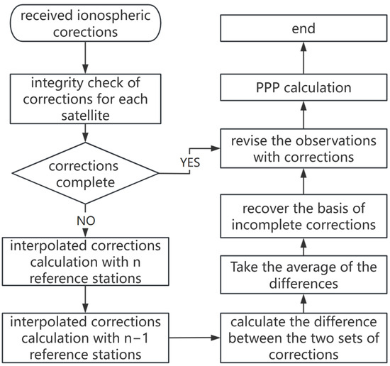 Figure 1. Flowchart of the basis recovery method.
3. Results
The dataset and the experimental results are presented in this subsection, along with the related discussion. The results of the experiment on the basis recovery algorithm and the experiment on the recommended number of reference stations are given in sequence.
3.1. Dataset
The experimental dataset was obtained from a continuously operating reference stations (CORS) network in North Carolina, USA, consisting of 26 stations in total. The regional station network was selected because the terrain in this area is flat, the density of the station network is relatively high, and the stations are distributed relatively uniformly. This enables the convenient selection of stations to form a network, thereby meeting the networking requirements for multiple experiments. Among these, 24 stations were designated as reference stations, while 3 stations were used to simulate user stations. Data were collected for the entire day of 9 April 2024, from 00:00 to 24:00, with a sampling interval of 5 s, and included dual-frequency observations from both the GPS and Galileo systems. The locations of the stations are shown in Figure 2. The ionospheric conditions during the observation period were stable, with no evident solar activity or large-scale geomagnetic changes. The signal-to-noise ratio and the rate of cycle slips in the observations were within normal ranges. It should be noted that the terrain of this area is relatively flat, and the atmospheric conditions on this day were inactive. These environmental conditions serve as the foundation for ensuring the validity and accuracy of conclusions. Different observational environments can potentially lead to deviations in experimental results. The experiment was conducted in two components: one for the validation of the basis recovery algorithm, and the other for determining the recommended number of reference stations.
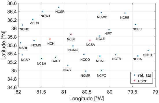
Figure 2.
Geographical distribution of the stations (blue dots represent reference stations, red asterisks represent user stations).
3.1.1. Experimental Data for the Basis Recovery Algorithm
The experiment involved four reference stations (NCLE, NCST, NCMO, and NCCO) and a user station (NCSA). The experiment assumes that the user station receives corrections for all satellites from the NCLE, NCST, and NCCO stations, while certain satellites are unable to obtain corrections from the reference station NCMO.
The basis of the corrections from reference station anomalies was recovered using the proposed method. These recovered corrections were then compared with those obtained by interpolation from all four reference stations to assess the feasibility of the proposed method. As the number of reference stations increases, the interpolation model error tends to decrease. To assess the lower bound of the proposed method’s reliability, the experiment was conducted using the minimum number of reference stations (only four). In this experiment, communication is assumed to be in a seamless state, meaning that potential unexpected long communication delays are not considered.
To further demonstrate the performance of the proposed method in practical PPP-RTK positioning, a PPP-RTK positioning experiment has been designed in the experiment section to compare the differences before and after applying the proposed method. Firstly, we present the performance of the proposed method on the Position Dilution of Precision (PDOP) throughout the day at the NCSA station. Subsequently, a PPP-RTK experiment is designed. To comprehensively show the ambiguity resolution performance at different startup times, the PPP engine is initiated every ten minutes starting from 0:20 to 23:30, utilizing 30 min of observational data for each run. The epoch interval is set at 5 s, and an attempt is made to fix ambiguities at each epoch. The evaluation indicators include the ambiguity fixing rate and the ratios for epochs where ambiguity resolution is successfully achieved. The ambiguity fixing rate is defined as the ratio of the number of epochs with fixed ambiguities to the total number of solved epochs.
3.1.2. Experimental Data for Assessing the Number of Reference Stations
As discussed earlier, the determination of the proper number of reference stations is inherently linked to the scale of the network. To comprehensively evaluate and provide recommendations for the proper number of reference stations, experiments were conducted using two large-scale networks with station spacings exceeding 100 km and two medium-to-small-scale networks with spacings between 30 and 50 km. The details of the four networks and the simulated rover stations are provided in Table 1, Table 2, Table 3 and Table 4, which also include the average distances between the reference and user stations. In addition, the distribution of reference stations can also affect the results of correction interpolation. Therefore, when reference station networks with different numbers of stations are selected, they are distributed as evenly as possible in all directions to achieve the greatest generalizability. Consequently, the applicability of the experiment conclusions will be limited to the premises, representing the most common and general conditions, namely, a flat terrain, an inactive period of the ionosphere, and evenly distributed reference stations.

Table 1.
A small-scale reference network with NCHI as the user station receives dual-frequency signals from the GPS/Galileo systems (Network A).
Table 2.
A small-scale reference network with NCSA as the user station receives dual-frequency signals from the GPS/Galileo systems (Network B).
Table 3.
A large-scale reference network with NCST as the user station receives dual-frequency signals from the GPS/Galileo systems (Network C).
Table 4.
A large-scale reference network with NCSA as the user station receives dual-frequency signals from the GPS/Galileo systems (Network D).
In the experimental section, the interpolated corrections for two GNSS systems were computed for each of the four networks. The corrections generated by the user station itself were used as the reference values for accuracy evaluation. This study focuses on the interpolation of ionospheric corrections, while the impact of inaccurate interpolated corrections on subsequent positioning results has been previously discussed in Wang et al. [25].
3.2. Experiment on the Basis Recovery Algorithm
This section first explores the feasibility of the basis recovery algorithm and demonstrates its performance. It should be noted that for the situation where all corrections are missing for one or more reference stations, a simple and clear explanation has already been provided in the method section. Therefore, the experimental section will only verify the situation where corrections for individual satellites are missing. It is assumed that the ionospheric delay corrections for all satellites at NCLE, NCST, and NCCO stations are successfully received, while the ionospheric delay corrections for each satellite at the NCMO station may be subject to reception failure. For each satellite at the user station NCSA, interpolation is performed for both scenarios: one where the NCMO station (with four reference stations) can provide the corrections, and the other where it cannot (with three reference stations). Due to differences in the frequencies and tracking methods of GPS and Galileo observations, the receiver-related hardware delays differ between the two systems. Consequently, the performance of the basis recovery algorithm is shown and evaluated separately for each system. The difference between the two sets of interpolated corrections is then calculated, and the results are statistically analyzed. Figure 3 and Figure 4 show the differences in L1 ionospheric corrections for all satellites in the GPS and Galileo systems, respectively.
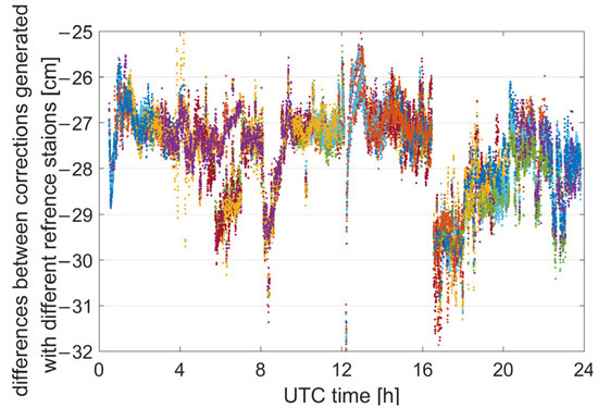
Figure 3.
Difference in interpolated L1 ionospheric corrections for all satellites in the GPS system using three and four reference stations.
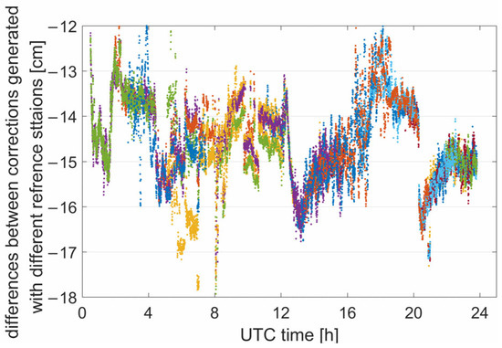
Figure 4.
Difference in interpolated L1 ionospheric corrections for all satellites in the Galileo system using three and four reference stations.
Based on Equation (12), the results of the two interpolations encompass both the interpolation model error and the difference in the linearly combined receiver hardware delay . Due to differences in observation frequencies and tracking methods between systems, exhibits system-dependent biases across different systems. Taking the results for all GPS satellites in Figure 3 as an example, the combined receiver hardware delays are consistent across all satellites, with the variations primarily governed by the interpolation model error . The interpolation model errors for all satellites are mostly confined to within 1 cm. The maximum error is approximately 2 to 3 cm, and its impact on ambiguity resolution is relatively limited given the wavelength of about 20 cm. Therefore, the basis recovery method of deriving through mean smoothing is supported by these findings. It should be clarified here that the interruptions observed in Figure 3 and Figure 4 were caused by the failure to fix ambiguities at multiple reference stations during those periods. This led to the inability to generate accurate atmospheric corrections. It is speculated that these failures might have been triggered by fluctuations in the quality of UPD products.
After extracting and compensating using the basis recovery algorithm, Figure 5 shows the difference between the L1 recovered ionospheric delay corrections for all satellites at the NCSA station using the proposed method with three reference stations and the ground-truth interpolated corrections with four reference stations. The ground-truth corrections refer to the corrections computed by fixing the coordinates of the reference stations to their known precise values. Figure 5 illustrates the different results for all GPS and Galileo satellites, with the systematic biases extracted and corrected. The recovered corrections differ from the ground-truth interpolated values only in , with errors remaining within a 2 cm fluctuation. The basis recovery method, however, preserves the valuable observations that would otherwise be discarded.
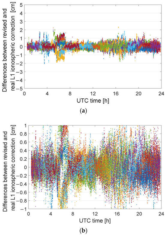
Figure 5.
Difference between the L1 recovered ionospheric delay corrections for all satellites at the NCSA station using three reference stations and the ground-truth interpolated corrections with four reference stations. (a) The range of the vertical axis is ±5 cm. (b) The range of the vertical axis is ±1 cm.
Furthermore, Figure 6 presents the probability distribution of the difference between the recovered corrections for all satellites at the NCSA station using the proposed method with three reference stations and the ground-truth interpolated corrections with four reference stations. Compared to the conventional discard strategy, the basis recovery algorithm generates a novel ionospheric delay correction, thereby improving the utilization of observations in PPP-RTK. The resulting ionospheric delay corrections deviate from the ground-truth interpolated values by no more than ±1 cm. This level of accuracy is adequate for PPP-RTK users [11].
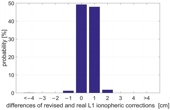
Figure 6.
Probability distribution of the difference between the recovered corrections and the true corrections.
Subsequently, a detailed account of the basis recovery method’s performance in the PPP-RTK positioning experiment will be provided. To begin with, the primary advantage of the proposed method lies in its ability to reinstate the usability of observations without corrections. When contrasted with the scenario where the method is not employed, there is an increase in the number of available observations. As a result, the satellite geometric distribution configuration becomes more favorable. Table 5 presents the proportion of epoch numbers with PDOP variations, as well as the PDOP improvement observed before and after the implementation of the proposed method.
Table 5.
Changes in DOP values before and after using the basis recovery method.
As indicated in Table 5, when utilizing the single GPS system and the GPS/Galileo system separately, the proportions of epochs with varying DOP are 5.16 and 8.79, respectively. Moreover, the PDOP declined to 1.58 and 1.08, corresponding to reduction rates of 14.1% and 6.9%, respectively. The aforementioned data offers a clear illustration of the proportions of epochs impacted by the proposed method, as well as the gains achieved in DOP values. Actually, when users are located in areas where GNSS signals are obstructed, i.e., in environments where the number of observable satellites significantly decreases, the additional observation information provided by the proposed method will offer greater benefits. In order to illustrate the minimum level of gains that this method can offer, the experiment was conducted without intentionally creating an obstructed setting. Rather, observation data from an open environment were employed. Table 5 illustrates the distinct gain patterns for single-system and multi-system configurations. It reveals that as the quantity of observable satellites increases, the additional observational data has a diminishing impact on the DOP gain. Consequently, if users find themselves in signal-constrained regions with a reduced number of observable satellites, the DOP gains they achieve are expected to exceed the results presented in Table 5.
The PPP-RTK experiment was conducted following the experiment design described in the dataset section. Table 6 displays the ambiguity fixing rate along with the average ratio for epochs where ambiguity has been successfully fixed (with a ratio greater than 2).
Table 6.
Ambiguity fixing rate along with the average ratio of PPP-RTK experiment.
As shown in Table 6, upon implementing the basis recovery method, the ambiguity fixing rate for the single GPS system rose by 0.9%, from 83.4% to 84.3%. Meanwhile, the fixing rate for the dual system experienced an increase of 0.5%, climbing from 89.25% to 89.75%. Furthermore, the mean ratio witnessed an improvement of 8.1% and 6.0% for the single GPS and dual system cases, respectively. The ambiguity fixing results, which are derived from tens of thousands of epochs over the full day, serve as compelling evidence of the proposed method’s efficacy. Additionally, it is reiterated that the experiment was based on observation data collected in an open environment. This setup showcases the minimum level of gains that the method can offer. In obstructed environments, ambiguity fixing is expected to bring about even more significant improvements.
3.3. Experiment on the Recommended Number of Reference Stations
In this section, in an observation environment characterized by relatively flat terrain and inactive atmospheric conditions, four reference station networks of varying scales were carefully chosen. Then, an in-depth study was conducted to determine the recommended number of reference stations for users positioned within each of these networks. In the investigation of the number of reference stations, the basis recovery algorithm was employed. To illustrate its effectiveness, the proportion of recovered corrections relative to the total number of corrections is calculated and presented for different networks.
The four reference station networks described in the dataset section are used to interpolate the ionospheric corrections for the user station. By regarding the ionospheric delays derived at the user stations as precise references, the errors of the interpolated ionospheric corrections are calculated. Subsequently, these errors are used to calculate the root mean square (RMS) statistical results. To emphasize again, when selecting surrounding reference stations for this experiment, we tried to ensure they were evenly distributed in all directions. The results are shown in Figure 7, Figure 8, Figure 9 and Figure 10. The reference station densities in Networks A and B are relatively dense, with inter-station distances predominantly clustered around 30 km and 50 km, respectively. As shown in Figure 7 and Figure 8, the interpolation error of the L1 ionospheric corrections decreases significantly with an average of four reference stations, while additional reference stations lead to only marginal improvements in the error reduction. Ionospheric delay corrections involve both code and phase ionospheric corrections for all observed satellites. However, with the addition of each reference station, the communication load increases, resulting in an inefficient use of resources. In small-scale networks with station spacings of 50 km or less, it is recommended to use four or five reference stations. For networks with a station spacing of 100 km, an increase in the number of stations to six or seven still results in a measurable improvement; however, the benefit becomes negligible when the station count reaches eight. For large-scale networks spanning over 100 km, the use of six or seven reference stations is recommended to provide correction interpolations.
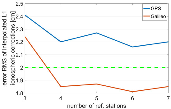
Figure 7.
RMS values of the L1 ionospheric correction interpolation errors for Network A with different numbers of stations.
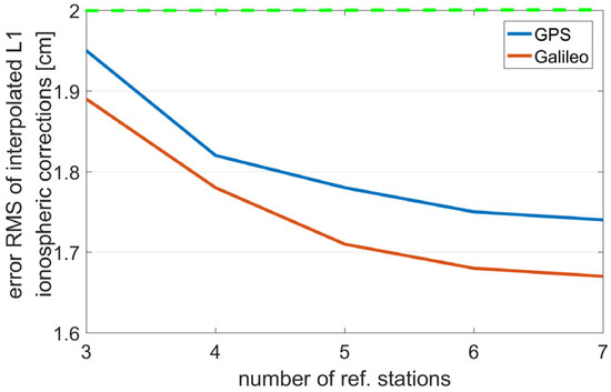
Figure 8.
RMS values of the L1 ionospheric correction interpolation errors for Network B with different numbers of stations.
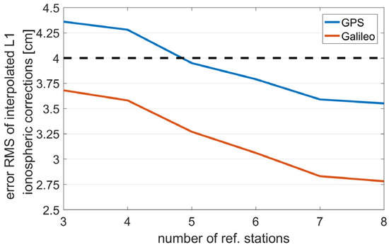
Figure 9.
RMS values of the L1 ionospheric correction interpolation errors for Network C with different numbers of stations.
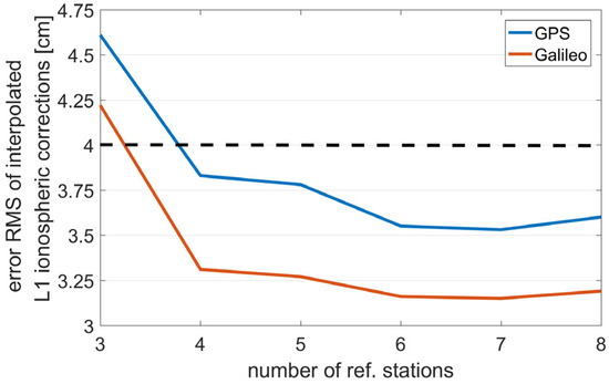
Figure 10.
RMS values of the L1 ionospheric correction interpolation errors for Network D with different numbers of stations.
As the number of reference stations utilized for interpolation grows, the quantity of corrections employed in the interpolation process also increases. This heightens the probability of a basis deficiency for these corrections. To conduct a more in-depth assessment of the performance of the proposed method, Table 7 displays the number of corrections used for basis recovery in reference station networks of varying scales, along with their proportion relative to the total number of corrections. It can be observed that, for large networks with 100 km station spacing, when the number of reference stations reaches seven, the interpolation basis recovery algorithm restores anomalous values, preserving approximately 3% of the total observations. The method effectively utilizes observations that would otherwise be discarded, improving the efficiency of data utilization. It must be reiterated here that the observational data employed in the experiment were obtained from a network of reference stations that were evenly distributed in a flat terrain during a period of low ionospheric activity, and a low-order surface interpolation model was used. Consequently, the experimental results are applicable to this most prevalent and generalized scenario. However, it should be noted that the outcomes may vary when the observation environment or the distribution of the reference stations changes. Additionally, we must acknowledge that while increasing the number of reference stations can enhance the accuracy of interpolation corrections, as suggested by our recommendations, users may sometimes find it impractical to access such a large number of nearby reference stations. For instance, there might only be three to five reference stations available within a certain range, as discussed in Section 3.2. Moreover, regarding the influence caused by interpolation correction errors of varying magnitudes on PPP-RTK results, one can consult Wang et al. [23].
Table 7.
Number (Num.) of recovered corrections and the proportion (Prop.) (%) of these corrections relative to the total number of corrections for different station networks with varying reference station densities.
4. Discussion
With the aim of engaging in a more in-depth discussion of the experimental results and showcasing their practical engineering significance, two auxiliary lines are added in Figure 7, Figure 8, Figure 9 and Figure 10: one in green (representing a 2 cm threshold) and the other in black (representing a 4 cm threshold). These two thresholds were determined based on empirical evidence. When the mean RMS of the corrections is less than 2 cm, the system can generally tolerate this level of error, having a minimal impact on the estimation results. Therefore, the corrections at this error level can be regarded as accurate, and users can directly employ the ionosphere-fixed model for calculations. When the RMS level falls between 2 cm and 4 cm, using the ionosphere-fixed model results directly may be influenced to a certain extent, with the degree of influence being related to factors such as the number of satellites and the satellite geometric configuration. In such cases, users can choose to use either the ionosphere-fixed or the ionosphere-constrained estimation model based on the observation situation. When the mean RMS exceeds 4 cm, the solution will be significantly affected, potentially leading to consequences such as a marked increase in parameter errors or failure in ambiguity resolution. In this scenario, it is recommended to adopt the ionosphere estimation model.
When users are in the process of selecting reference stations for interpolating corrections, the first step is to examine the quantity of correction numbers offered by each reference station. Owing to issues like observation data quality and IAR, the number of corrections from certain individual reference stations may be significantly lower than that of their stations. These potentially unreliable reference stations must be excluded during the selection. Next, users should strive to select a set of reference stations that are not only close but also evenly distributed. This arrangement is crucial for ensuring that the quality of the interpolated corrections is optimized. Finally, users should aim to pick reference stations in a number that aligns with the recommended quantity specified in this paper. In summary, on the premise of ensuring that the quality and quantity of the corrections provided by the selected reference stations remain normal, among the group of reference stations nearest to the user (which implies that the distances between these reference stations and the user should not differ significantly), one should strive to select the recommended number of reference stations in different azimuths relative to the user. In the case of a sparse station network, it is necessary to choose at least three reference stations, ensuring that the user is located within the Delaunay triangle formed by these three stations.
5. Conclusions
Interpolating ionospheric delay corrections at the user station, extracted from reference stations, plays a crucial role in PPP-RTK applications. In non-specific environments, the quality of interpolated corrections depends not only on the choice of the interpolation model but also on the reference stations used in the interpolation process. Furthermore, determining the number of reference stations based on the size of the reference network and mitigating correction losses from individual stations that result in the unavailability of interpolated corrections and consequently lead to the wastage of observations, are two crucial factors to address.
This study models and analyzes two common scenarios of correction loss, with particular emphasis on the situation where the loss of corrections for certain satellites at a single reference station causes discrepancies between the interpolated corrections and those of other satellites, leading to the exclusion of observations. To address this problem, the basis recovery algorithm is proposed. The algorithm effectively extracts and compensates for the combined receiver hardware delay in ionospheric delay interpolation. With this method, even if the corrections for a satellite are lost at a specific reference station, they can still be interpolated and compensated, ensuring the observation remains usable. The experimental results validated the feasibility of the algorithm, showing that the model interpolation errors are minimal, with the majority confined to within 1 cm. Furthermore, the linearly combined receiver hardware delays exhibit a consistent pattern across the satellites. The recovered ionospheric delay corrections obtained through the algorithm deviate from the accurate interpolated (calculated using a sufficient number of reference stations) values by no more than ±1 cm. This level of accuracy is adequate for PPP-RTK users. Furthermore, approximately 3% of the observations, which would otherwise have been discarded due to the missing corrections from a specific reference station, are retained by the algorithm.
Owing to the limitations in the accuracy of the interpolation model, increasing the number of reference stations beyond a certain threshold does not improve the interpolation precision; rather, it leads to a higher communication load. The threshold also depends on the size of the reference network. In this study, in the case of flat terrain, stable atmospheric conditions, and relatively uniform distribution of reference stations in all directions, the selection of the number of reference stations was analyzed across four reference networks when using the low-order surface interpolation model, each varying in scale and station density. Here, it is once again emphasized that the experimental conclusions are directly linked to the observational environment. The background circumstances assumed in this work represent the most general and widely applicable scenarios. In networks with station spacings of 30 km and 50 km, a notable reduction in interpolation error is observed when the number of reference stations reaches four, while additional increases in the number of stations result in only marginal improvements. For small networks with a station spacing of 50 km, the use of four or five reference stations is recommended. In contrast, for larger networks with a station spacing of 100 km, it is advisable to employ six or seven reference stations.
In conclusion, it is essential to highlight that the research in this work regarding the recommended number of reference stations focuses on ionospheric delay. With regard to the subject matter pertaining to tropospheric delay, it warrants further exploration and discussion.
Author Contributions
Conceptualization, R.T.; Methodology, S.W. and R.Z.; Software, S.W.; Validation, L.F. and X.L.; Writing—original draft, R.Z.; Supervision, R.T. and L.F.; Project administration, X.L. All authors have read and agreed to the published version of the manuscript.
Funding
This research was funded by the National Science Foundation for Young Scientists of China (Grant No. 42104020), the National Natural Science Foundation of China (Grant No. 12203060), and the Youth Innovation Promotion Association CAS (Grant No. 2023426).
Data Availability Statement
Some or all data, models, or code generated or used during the study are available from the corresponding author by request.
Acknowledgments
The authors would like to thank the IGS for supporting precise products. The authors are grateful to the American National Oceanic and Atmospheric Administration (NOAA) for the CORS data sharing platform.
Conflicts of Interest
The authors declare no conflict of interest regarding the publication of this paper.
References
- Héroux, P.; Kouba, J. GPS precise point positioning using IGS orbit products. Phys. Chem. Earth Part A-Solid Earth Geod. 2001, 26, 573–578. [Google Scholar] [CrossRef]
- Zumberge, J.F.; Heflin, M.B.; Jefferson, D.C.; Watkins, M.M.; Webb, F.H. Precise point positioning for the efficient and robust analysis of GPS data from large networks. J. Geophys. Res. Solid Earth 1997, 102, 5005–5017. [Google Scholar] [CrossRef]
- Geng, J.; Teferle, F.N.; Meng, X.; Dodson, A.H. Towards PPP-RTK: Ambiguity resolution in real-time precise point positioning. Adv. Space Res. 2011, 47, 1664–1673. [Google Scholar] [CrossRef]
- Laurichesse, D.; Mercier, F.; Berthias, J.P.; Broca, P.; Cerri, L. Integer ambiguity resolution on undifferenced GPS phase measurements and its application to PPP and satellite precise orbit determination. Navigation 2009, 56, 135–149. [Google Scholar] [CrossRef]
- Collins, P.; Lahaye, F.; Heroux, P.; Bisnath, S. Precise Point Positioning with Ambiguity Resolution using the Decoupled Clock Model. In Proceedings of the 21st International Technical Meeting of the Satellite Division of The Institute of Navigation (ION GNSS 2008), Savannah, GE, USA, 16–19 September 2008. [Google Scholar]
- Ge, M.; Gendt, G.; Rothacher, M.; Shi, C.; Liu, J. Resolution of GPS carrier-phase ambiguities in Precise Point Positioning (PPP) with daily observations. J. Geod. 2008, 82, 389–399. [Google Scholar] [CrossRef]
- Geng, J.; Meng, X.; Dodson, A.H.; Teferle, F.N. Integer ambiguity resolution in precise point positioning: Method comparison. J. Geod. 2010, 84, 569–581. [Google Scholar] [CrossRef]
- Wübbena, G.; Bagge, A.; Schmitz, M. RTK Networks based on Geo++® GNSMART- Concepts, Implementation, Results. In Proceedings of the 14th International Technical Meeting of the Satellite Division of The Institute of Navigation (ION GPS 2001), Salt Lake City, UL, USA, 11–14 September 2001. [Google Scholar]
- Wübbena, G.; Schmitz, M.; Bagge, A. PPP-RTK: Precise Point Positioning Using State-Space Representation in RTK Networks. In Proceedings of the 18th International Technical Meeting of the Satellite Division of The Institute of Navigation (ION GNSS 2005), Long Beach, CA, USA, 13–16 September 2005. [Google Scholar]
- Li, X.; Huang, J.; Li, X.; Lyu, H.; Wang, B.; Xiong, Y.; Xie, W. Multi-constellation GNSS PPP instantaneous ambiguity resolution with precise atmospheric corrections augmentation. GPS Solut. 2021, 25, 107. [Google Scholar] [CrossRef]
- Li, X.; Zhang, X.; Ge, M. Regional reference network augmented precise point positioning for instantaneous ambiguity resolution. J. Geod. 2011, 85, 151–158. [Google Scholar] [CrossRef]
- Odijk, D.; Zhang, B.; Khodabandeh, A.; Odolinski, R.; Teunissen, P.J.G. On the estimability of parameters in undifferenced, uncombined GNSS network and PPP-RTK user models by means of S-system theory. J. Geod. 2016, 90, 15–44. [Google Scholar] [CrossRef]
- Teunissen, P.J.G.; Odijk, D.; Zhang, B. PPP-RTK: Results of CORS network-based PPP with integer ambiguity resolution. J. Aeronaut. Astronaut. Aviat. Ser. A 2010, 42, 223–230. [Google Scholar]
- Zhang, B.; Teunissen, P.J.G.; Odijk, D. A Novel Un-differenced PPP-RTK Concept. J. Navig. 2011, 64, S180–S191. [Google Scholar] [CrossRef]
- Amalfitano, D.; Cutugno, M.; Robustelli, U.; Pugliano, G. Designing and Testing an IoT low-cost PPP-RTK augmented GNSS Location device. Sensors 2024, 24, 646. [Google Scholar] [CrossRef] [PubMed]
- Robustelli, U.; Cutugno, M.; Pugliano, G. Low-Cost GNSS and PPP-RTK: Investigating the Capabilities of the u-blox ZED-F9P Module. Sensors 2023, 23, 6074. [Google Scholar] [CrossRef]
- Montenbruck, O.; Steigenberger, P.; Hauschild, A. Broadcast versus precise ephemerides: A multi-GNSS perspective. GPS Solut. 2015, 19, 321–333. [Google Scholar] [CrossRef]
- Gu, S.; Gan, C.; He, C.; Lyu, H.; Hernandez-Pajares, M.; Lou, Y.; Geng, J.; Zhao, Q. Quasi-4-dimension ionospheric modeling and its application in PPP. Satell. Navig. 2022, 3, 24. [Google Scholar] [CrossRef]
- Odolinski, R.; Teunissen, P.J.G. An assessment of smartphone and low-cost multi-GNSS single-frequency RTK positioning for low, medium and high ionospheric disturbance periods. J. Geod. 2019, 93, 701–722. [Google Scholar] [CrossRef]
- Gao, Y.; Li, Z.; McLellan, J.F. Carrier Phase Based Regional Area Differential GPS for Decimeter-Level Positioning and Navigation. In Proceedings of the 10th International Technical Meeting of the Satellite Division of The Institute of Navigation (ION GPS 1997), Kansas City, MI, USA, 16–19 September 1997. [Google Scholar]
- Han, S.; Rizos, C. GPS Network design and error mitigation for real-time continuous array monitoring systems. In Proceedings of the 9th International Technical Meeting of the Satellite Division of The Institute of Navigation (ION GPS 1996), Kansas City, MI, USA, 17–20 September 1996. [Google Scholar]
- Wübbena, G.; Bagge, A.; Seeber, G.; Böder, V.; Hankemeier, P. Reducing distance dependent errors for real-time precise DGPS applications by establishing reference station networks. In Proceedings of the 9th International Technical Meeting of the Satellite Division of The Institute of Navigation (ION GPS 1996), Kansas City, MI, USA, 17–20 September 1996. [Google Scholar]
- Wang, S.; Li, B.; Gao, Y.; Gao, Y.; Guo, H. A comprehensive assessment of interpolation methods for regional augmented PPP using reference networks with different scales and terrains. Measurement 2020, 150, 107067. [Google Scholar] [CrossRef]
- Wang, M.; Gao, Y. An Investigation on GPS Receiver Initial Phase Bias and Its Determination. In Proceedings of the 2007 National Technical Meeting of The Institute of Navigation, San Diego, CA, USA, 22–24 January 2007. [Google Scholar]
- Wang, S.; Li, B.; Ge, H.; Zhang, Z. Algorithm and Assessment of Ambiguity-Fixed PPP with BeiDou Observations and Regional Network Augmentation. J. Surv. Eng. 2020, 146, 04020009. [Google Scholar] [CrossRef]
- Rovera, G.D.; Torre, J.M.; Sherwood, R.; Abgrall, M.; Courde, C.; Laas-Bourez, M.; Uhrich, P. Link calibration against receiver calibration: An assessment of GPS time transfer uncertainties. Metrologia 2014, 51, 476–490. [Google Scholar] [CrossRef]
- Odijk, D. Fast Precise GPS Positioning in the Presence of Ionospheric Delays. Ph.D. Thesis, Delft University of Technology, Delft, The Netherlands, 2002. [Google Scholar]
- Khodabandeh, A. Single-station PPP-RTK: Correction latency and ambiguity resolution performance. J. Geod. 2011, 95, 42. [Google Scholar] [CrossRef]
- Melbourne, W.G. The case for ranging in GPS-based geodetic systems. In Proceedings of the First International Symposium on Precise Positioning with the Global Positioning System: Positioning with GPS—1985, Rockville, MA, USA, 15–19 April 1985; U.S. Department of Commerce: Rockville, MA, USA, 1985; pp. 373–386. [Google Scholar]
- Wübbena, G. Software developments for geodetic positioning with GPS using TI-4100 code and carrier measurements. In Proceedings of the First International Symposium on Precise Positioning with the Global Positioning System: Positioning with GPS—1985, Rockville, MA, USA, 15–19 April 1985; U.S. Department of Commerce: Rockville, MA, USA, 1985; pp. 403–412. [Google Scholar]
- Li, X.; Li, X.; Yuan, Y.; Zhang, K.; Zhang, X.; Wickert, J. Multi-GNSS phase delay estimation and PPP ambiguity resolution: GPS, BDS, GLONASS, Galileo. J. Geod. 2018, 92, 579–608. [Google Scholar] [CrossRef]
- Wang, S.; Li, B.; Li, X.; Zang, N. Performance analysis of PPP ambiguity resolution with UPD products estimated from different scales of reference station networks. Adv. Space Res. 2018, 61, 385–401. [Google Scholar] [CrossRef]
Disclaimer/Publisher’s Note: The statements, opinions and data contained in all publications are solely those of the individual author(s) and contributor(s) and not of MDPI and/or the editor(s). MDPI and/or the editor(s) disclaim responsibility for any injury to people or property resulting from any ideas, methods, instructions or products referred to in the content. |
© 2025 by the authors. Licensee MDPI, Basel, Switzerland. This article is an open access article distributed under the terms and conditions of the Creative Commons Attribution (CC BY) license (https://creativecommons.org/licenses/by/4.0/).