Remote Estimation of Above-Ground Biomass Throughout the Entire Growth Period for Crops with Conspicuous Spikes

Abstract

Above-ground biomass (AGB) is an important factor in crop yield. However, most AGB estimation methods for crops with conspicuous spikes, such as rice and sorghum, can achieve high accuracy during the vegetative stage but low accuracy during the reproductive stage. In this study, we explored an AGB estimation model throughout the entire growth period. Firstly, we divided the growth period of crops into two stages—before heading and after heading—and adopted different strategies according to the characteristics of the different stages. Before heading, we estimated AGB by multiplying the multi-spectral vegetation index (VI) and the crop canopy height (H) square. After heading, we added spectral absorption characteristic parameters to characterize spike biomass and used a multiple linear regression model. This model can accurately estimate AGB in both rice and sorghum throughout the entire growth period, which has a coefficient of determination (R²) above 0.88 and the relative root mean square error (rRMSE) below 20.13% in both crops. Compared with the direct estimation of AGB throughout the entire growth period using H² × VI, this model effectively improved the accuracy of AGB estimation for crops with conspicuous spikes in the reproductive stage, which can provide reliable information for evaluating crop growth at plot scale.

1. Introduction

AGB is a key growth parameter for evaluating the crop growth situation, which reflects the weight of organic matter accumulated by the crop after photosynthesis, and can be used to evaluate the net productivity of the crop [1]. The traditional method of acquiring AGB is destructive field measurement, which mainly obtains AGB through manual destructive sampling, drying processes, and integration with manual measurements. This method is time-consuming and labor-intensive, inefficient, and will damage crop plants, so it is impossible to continuously observe the same crop plant. Crop growth is a dynamic and continuous process, and it is necessary to continuously analyze the growth parameters of the crop at different growth stages to monitor crop growth, so the traditional method of obtaining growth parameters obviously cannot meet this requirement. Compared with time-consuming and labor-intensive destructive manual observation, remote sensing technology is mainly based on the spectral characteristics of crop plants, which offers advantages such as fast, non-destructive, and continuous observation [2].

There are various remote sensing estimation methods for crop AGB, including multi-spectral data [3,4], hyperspectral data [5,6], and lidar data [7,8]. According to the estimation principle, these can be divided into mechanism models [9] and empirical models [10].

Mechanism models include the crop growth model [11], the light energy utilization model [12], and the canopy radiation transfer model (RTM) [13]. The crop growth model simulates the growth process of crops through environmental information such as meteorology, soil, planting density, and planting methods, as well as biological information such as crop variety characteristics, then simulates the changes in volume and mass of crops during the growth process to estimate crop AGB [14]. Common mechanism models include the decision support system for agrotechnology (DSSAT) model [15,16,17,18,19], the World Food Study (WOFOST) model [20,21,22] and the agricultural product system simulator (APSIM) model [23,24,25,26]. The light energy utilization model uses the light energy utilization rate as the efficiency of crop dry matter accumulation during a certain period of time [27]. Common light energy utilization models include the Carnegie–Ames–Stanford approach (CASA) model [28,29,30] and the global production efficiency model (GLO-PEM) [31]. RTM is a physical remote sensing method, based on physical principles and mathematical equations, that is used to explain the canopy’s radiation transfer process [32]. The PROSAIL model, one of the major RTMs, has been widely applied to the inversion of biochemical variables and biophysical parameters of vegetation, such as the leaf area index (LAI) [33] and AGB [34]. However, the mechanism model is a model based on relatively complex biological theories, which requires a large amount of environmental information, accurate crop information, and complex biological theories as support, and the modeling process is rather complicated.

Empirical models generally do not pay attention to the internal mechanism of the crop growth process, but directly establish the relationship between crop surface reflectance, vegetation index (VI), or geometric parameters and crop growth parameters according to the spectral characteristics of crops, and estimate crop growth parameters based on statistical models. In this study, empirical models are divided into AGB estimation models based on multispectral data [35], estimation models based on hyperspectral data [36], estimation models based on texture information [37], and estimation models integrating multiple data sources according to different feature parameters used in the models [38,39].

VI calculated from multispectral data is a common method to estimate AGB, which mainly carries out statistical analysis on crop AGB and corresponding VI of different growth periods or entire growth periods to obtain the best regression model [40,41,42]. The hyperspectral data have higher spectral resolution, providing more accurate crop reflectance and also allowing the spectral curve of the crop to be obtained, which can also allow the crop to be observed in a detailed and comprehensive way [43,44]. Feng et al. [45] applied hyperspectral data to deep learning and proposed a VGC-AGB model to improve the accuracy of potato AGB estimation. Texture information is the embodiment of the change rule of image on the gray scale, which can well reflect the structural characteristics of crop canopy in the horizontal direction [46,47,48,49]. Fu et al. [50,51] found that the introduction of Gabor texture into the spectral index model could improve the estimation accuracy of winter wheat nitrogen content. Liu et al. [52] improved the estimation accuracy of rice AGB by changing the window size and direction of the grey level co-occurrence matrix GLCM, with R² reaching 0.84.

Although different types of data have been introduced for estimating crop AGB, when only a single type of data is used to estimate crop AGB, various problems often arise. For example, when crop AGB is estimated by using texture information, most texture indexes are weakly correlated with the AGB in the early period of crop growth [46]. Therefore, many studies have combined different types of data to estimate crop AGB, such as VI, texture index, canopy height, and vegetation coverage. Jimenez-Berni et al. [53] used a LiDAR sensor to extract three-dimensional geometric information of wheat, then obtained wheat plant height and vegetation coverage. They combined plant height with vegetation coverage to estimate wheat AGB, with R² reaching 0.92. Tilly et al. [54] used a ground-based laser scanner to obtain wheat plant height and combined it with ground-measured spectrum, finding that the combination of the two can effectively improve the accuracy of estimating AGB. Yue et al. [55] found that the correlation between VI multiplied by height and wheat AGB was higher than that between single VI or height and AGB. Navarro et al. [56] used the RGB image of an unmanned aerial vehicle (UAV) to extract a three-dimensional point cloud, then combined it with Sentinel-1 SAR and Sentinel-2 optical images, and found that the estimation model established by the combination of the three had the highest accuracy. Shu et al. [57] used UAV digital surface model (DSM) images to extract maize plant height, then multiplied the VI and plant height to characterize LAI. Finally, they multiplied LAI and plant height to build an AGB cube model, with R² reaching 0.79 and the relative root mean square error (rRMSE) reaching 29.19%. Liu et al. [58,59] combined UAV RGB data with hyperspectral data to estimate potato AGB, effectively reducing the root mean square error (RMSE). Liu et al. [60] combined remote sensing features with structural features to estimate wheat AGB, with R² reaching 0.88.

However, despite fusing different types of data, the effects of most crop AGB estimation methods are still relatively poor during the heading stage and subsequent growth stages, especially for crops with conspicuous spikes. Miao et al. [61] divided the growth period of rice into four stages from the tillering stage to the heading stage, and used the optimal multi-narrowband reflectance (OMNBR) model based on the original reflectance of hyperspectral data, R² reached 0.77 at the tillering stage and 0.50 at the heading stage. Xu et al. [62] used VI combined with the corresponding-band texture (VI-CBT) to explore the effect of the fusion characteristics of VI and texture in estimating the AGB of rice at different growth stages. The effect was good at the tillering and jointing stages, but began to deteriorate after the booting stage. As a crop with conspicuous spikes, the presence of spikes in rice during the booting stage and subsequent growth stages can affect the canopy spectrum. Moreover, most of the existing crop AGB estimation methods are based on leaf biomass and rarely take spike biomass into account, which leads to a significant decline in the AGB estimation effect starting from the booting stage, especially at the heading stage. There is a lack of effective methods for estimating crop AGB in the heading stage and subsequent growth stages, especially for crops with conspicuous spikes. Therefore, a crop AGB estimation method is needed that takes into account both the composition of the crop canopy structure and the spectral changes of the canopy before and after heading. The main objectives of the study are to (1) evaluate the necessity of introducing hyperspectral features to improve the estimation of AGB of crops with conspicuous spike after heading; (2) find a spectral feature that can better characterize the spike biomass to improve the estimation accuracy of AGB; and (3) compare the effects of different methods in estimating the AGB of crops with conspicuous spikes after heading and propose a crop AGB estimation method based on the entire growth period.

2. Materials and Methods

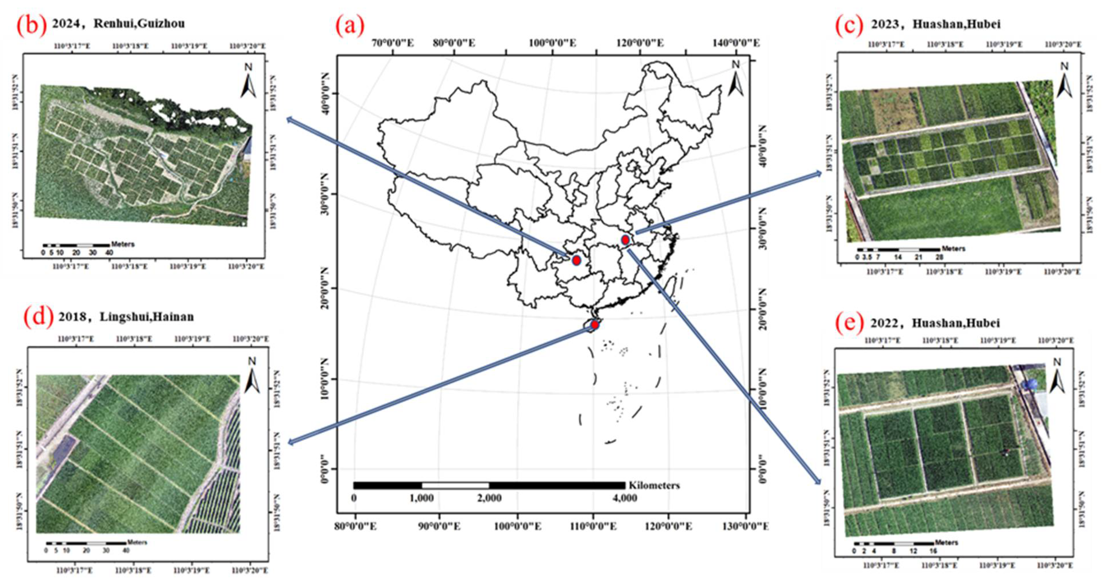
2.1. Study Area

There were two rice study areas in this study: the hybrid rice experiment base of Wuhan University in Lingshui, Hainan province, China (18°31′N, 110°3′E), and that in Wuhan, Hubei province, China (30°33′N, 114°32′E). 1. The two rice study areas are in different climatic zones, which have disparate meteorological conditions. Hainan is located in the tropics and has a tropical monsoon climate with high temperatures throughout the year, while Hubei belongs to the subtropics and has a subtropical monsoon climate with an annual average temperature of 15.8 °C. In Hubei, rice plants were usually sown in mid-May, transplanted in early June, and harvested in October, with a growth period of around 4 months. By contrast, rice plants in Hainan were sown in mid-December of the previous year, transplanted in early January, and harvested in May, with a growth period of around 5 months. At the same time, there is also a sorghum study area in Zunyi, Guizhou province, China (27°42′N, 106°22′E). Guizhou province has a subtropical humid monsoon climate with moderate rainfall and an average annual temperature of 15.8 °C. The planting time of sorghum varies due to the significant difference in altitude. In this study, sorghum was planted in late March and harvested in late August.

As shown in Figure 1, there were 42 cultivars in 2018 Hainan, 27 cultivars in 2022 Hubei, 48 cultivars in 2023 Hubei, and 54 cultivars in 2024 Guizhou. Each cultivar had a separate field plot, and the white mark placed at the edge of the plots was used to distinguish different cultivars.

2.2. AGB Measurements

The collection of crop AGB began at the initial stage of tillering and continued until the wax ripening stage. During each sampling, three representative crop plants were randomly selected from each experimental plot, then the crop was shoveled out and put into the sampling bag. After the sampling bags were numbered, a small amount of field water was placed in the sampling bag to ensure the survival of the crop. The leaves, stems, and spikes of the crop were numbered and sealed in separate paper bags, then dried in an oven at 105 °C for 30 min, which was then adjusted to 80 °C for about two days at a constant temperature until the weight remained the same. At the end of drying, each sample was weighed separately and recorded. The leaf, stem, and spike biomass in the same plot were added to obtain three crop plants in the field total AGB (g). The AGB conversion formula for this cell is shown in Equation (1), and the unit of AGB is g/m².

$$\mathrm{A}\mathrm{G}\mathrm{B}={\displaystyle \frac{\mathrm{W}}{3}}\times \mathrm{d}$$

(1)

where $\mathrm{W}$ is the total three crop plants biomass of each plot (g) and $\mathrm{d}$ is the planting density of each plot (strains/ m²).

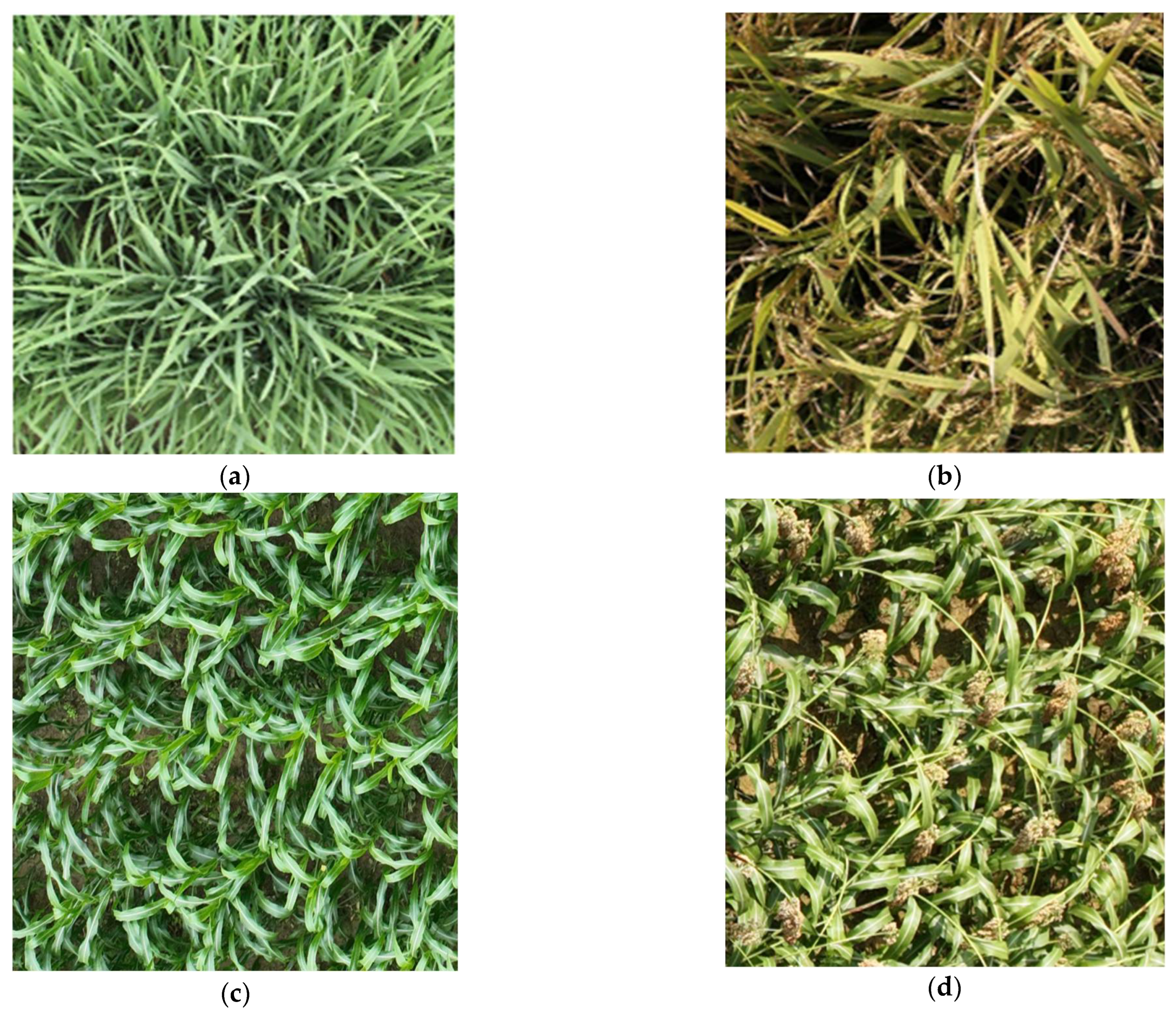
2.3. Manual Determination of Heading Date in Crop

The heading date in crops is generally defined as the time when approximately 50% of the spikes have exserted, which was determined by manual visual observations in the field. The heading date of the studied different crop cultivars varied between 59 and 73 Days After Transplanting (DAT) in rice. In this study, the growing season of each crop cultivar can be roughly divided based on heading date into before-heading and after-heading stages.

2.4. Canopy Hyperspectral Reflectance Retrieved from ASD

The ground hyperspectral data were collected using an Analytical Spectral Device (ASD). The ASD FieldSpec4 (Analytical Spectral Devices, Inc., West Gosford NSW, Malvern Panalytical, Worcs, UK) spectrometer has a spectral resolution of 350 nm~2500 nm and a spectral resolution of 3 nm in the range of 350 nm~1000 nm. The spectral resolution in the 1000 nm~2500 nm wave range is 8 nm. The instrument can be used to measure a variety of parameters such as reflectivity, transmittance, radiant brightness, and radiance.

2.5. UAV-Based Data Collection

Before the UAV imaging, the ground control points (GCPs) were evenly arranged in the field using black and white calibration plates measuring 40 cm in length and width. Intelligent real-time kinematic (RTK) was used to obtain the accurate geographical positions of each control point. UAV images were collected throughout the entire growth period in 2018 Hainan, 2022 Hubei, 2023 Hubei, and 2024 Guizhou. The 12-band multispectral images were obtained for the study site on the first flight, and the RGB images were then taken on the other flight.

The UAV data used in this study include RGB and multispectral images. The RGB images were used to extract canopy height, and the multispectral images were used to extract VI.

2.5.1. RGB Image

The RGB images of the study site were taken with a DJI FC 6310R camera mounted on a DJI Phantom 4 RTK UAV (SZ DJI Technology Co., Ltd., Shenzhen, China). The UAV is equipped with an adjustable cloud terrace (pitch angle ranges from +30° to −90°). The horizontal field of view of the camera was 84°, the vertical field of view of the camera was ±10°, and the ground sampling distance (GSD) was 0.8 cm. The flight altitude was 30 m above ground level. The forward overlap was set to 85%, and the lateral overlap was set to 80%.

2.5.2. Multispectral Image

The 12-band images of the study site were obtained by the Mini-MCA camera system (Tetracam, Inc., Chatsworth, CA, USA) mounted on an M8 UAV (Beijing TT Aviation Technology Co., Ltd, Beijing, China). This array of 12 cameras was equipped with customer-specified band pass filters centered at a wavelength of 490 nm, 520 nm, 550 nm, 570 nm, 670 nm, 680 nm, 700 nm, 720 nm, 800 nm, 850 nm, 900 nm, and 950 nm, respectively. The 12 camera lenses were co-registered in the laboratory prior to the flight so that corresponding pixels of each lens were spatially overlapping in the same focal plane. The flights were taken in sunny and cloudless weather between 10:00 AM and 2:00 PM at an altitude of 100 m and with an image spatial resolution of 5.5 cm.

For image radiometric calibration, a linear relationship was assumed between surface reflectance ($\mathsf{\rho }$) and image digital numbers (DNs):

$${\mathsf{\rho }}_{\mathsf{\lambda }}={\mathrm{D}\mathrm{N}}_{\mathsf{\lambda }}\times {\mathrm{G}\mathrm{a}\mathrm{i}\mathrm{n}}_{\mathsf{\lambda }}+{\mathrm{O}\mathrm{f}\mathrm{f}\mathrm{s}\mathrm{e}\mathrm{t}}_{\mathsf{\lambda }}$$

(2)

where ${\mathsf{\rho }}_{\mathsf{\lambda }}$ and ${\mathrm{D}\mathrm{N}}_{\lambda }$ were the surface reflectance and corresponding image digital numbers at wavelength $\lambda$. Eight near-Lambertian calibration canvases, at the constant reflectance of 0.03, 0.06, 0.12, 0.24, 0.36, 0.48, 0.56, and 0.80, were placed in the camera’s field of view to solve ${\mathrm{G}\mathrm{a}\mathrm{i}\mathrm{n}}_{\mathsf{\lambda }}$ and ${\mathrm{O}\mathrm{f}\mathrm{f}\mathrm{s}\mathrm{e}\mathrm{t}}_{\mathsf{\lambda }}$ value in different bands using the least square method for image radiometric calibration. In this case, the canopy reflectance at 12 bands can be calculated based on Equation (2).

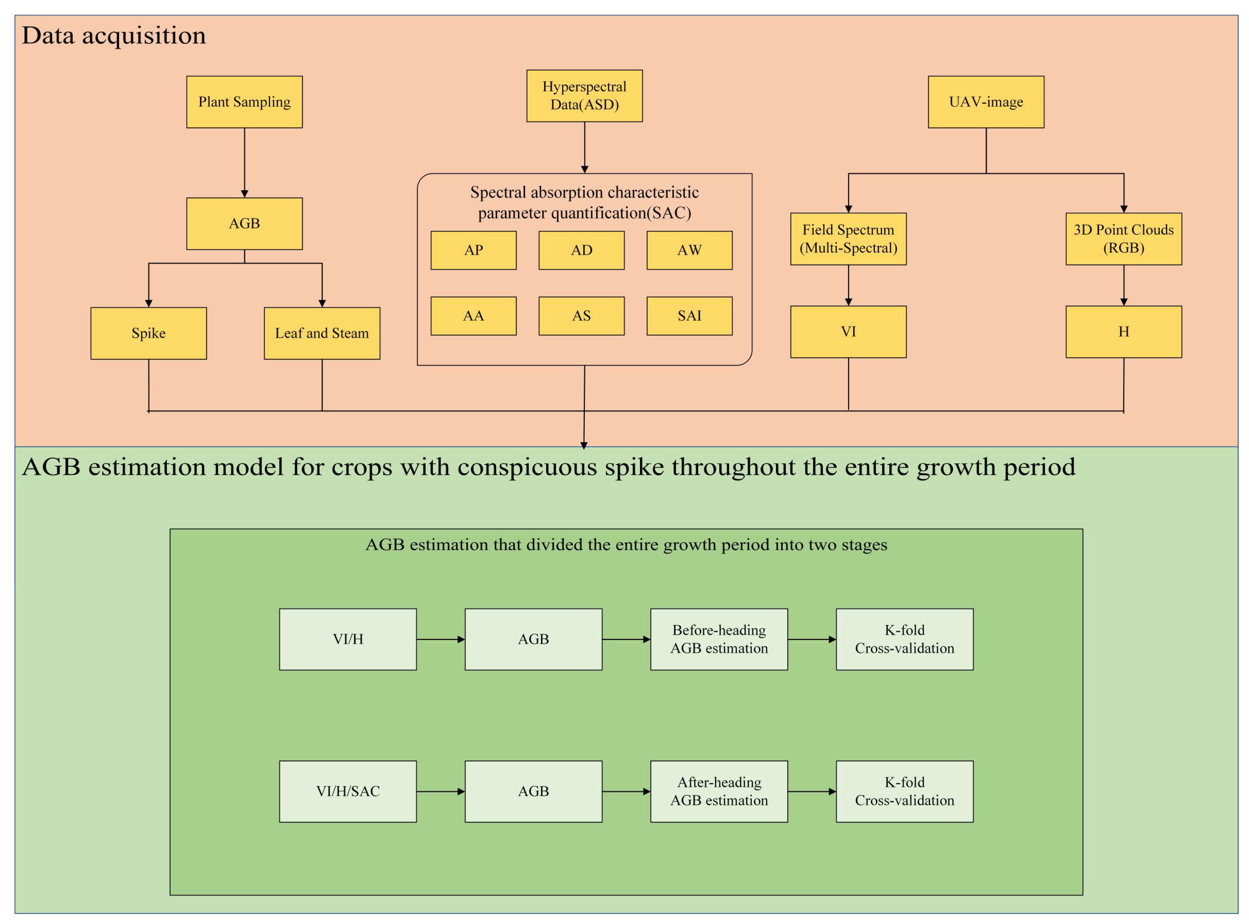
2.6. Features Derived from Remote Sensing Data

For each crop plot, a rectangular region of interest (ROI) of the same size was defined that maximally fit the plot. The ROI included three rows of crops, corresponding to around 800 pixels in the 12-band image and 2000 pixels in the RGB image. The actual area of each area is 2.42 m², accounting for approximately 70% of the area of a single plot. The average reflectance and the average height of all pixels within the ROI were taken as the plot-level canopy reflectance and canopy height, respectively, which correspond to the AGB at the field level.

2.6.1. VI

The plot-level VI was calculated from plot-level canopy reflectance. Four VIs, which are widely used for AGB estimation in many studies and can be easily applied in current satellite sensors, were used in this study for AGB estimation (

Table 1. VI calculated from UAV images in this study.

Features	Description	Equation
NDVI [63]	Normalized difference vegetation index	$({\mathsf{\rho }}_{\mathrm{N}\mathrm{I}\mathrm{R}}-{\mathsf{\rho }}_{\mathrm{R}\mathrm{e}\mathrm{d}})/({\mathsf{\rho }}_{\mathrm{N}\mathrm{I}\mathrm{R}}+{\mathsf{\rho }}_{\mathrm{R}\mathrm{e}\mathrm{d}})$
EVI2 [64]	Two-band enhanced vegetation index	$2.5\times {\displaystyle \frac{{\mathsf{\rho }}_{\mathrm{N}\mathrm{I}\mathrm{R}}-{\mathsf{\rho }}_{\mathrm{R}\mathrm{e}\mathrm{d}}}{{\mathsf{\rho }}_{\mathrm{N}\mathrm{I}\mathrm{R}}+2.4\times {\mathsf{\rho }}_{\mathrm{R}\mathrm{e}\mathrm{d}}+1}}$
NDRE [65]	Normalized difference red-edge vegetation index	$({\mathsf{\rho }}_{\mathrm{N}\mathrm{I}\mathrm{R}}-{\mathsf{\rho }}_{\mathrm{R}\mathrm{e}\mathrm{d}\mathrm{E}\mathrm{d}\mathrm{g}\mathrm{e}})/({\mathsf{\rho }}_{\mathrm{N}\mathrm{I}\mathrm{R}}+{\mathsf{\rho }}_{\mathrm{R}\mathrm{e}\mathrm{d}\mathrm{E}\mathrm{d}\mathrm{g}\mathrm{e}})$
OSAVI [66]	Optimized soil adjusted vegetation index	$(1+0.16)\times {\displaystyle \frac{{\mathsf{\rho }}_{\mathrm{N}\mathrm{I}\mathrm{R}}-{\mathsf{\rho }}_{\mathrm{R}\mathrm{e}\mathrm{d}}}{{\mathsf{\rho }}_{\mathrm{N}\mathrm{I}\mathrm{R}}+{\mathsf{\rho }}_{\mathrm{R}\mathrm{e}\mathrm{d}}+0.16}}$

).

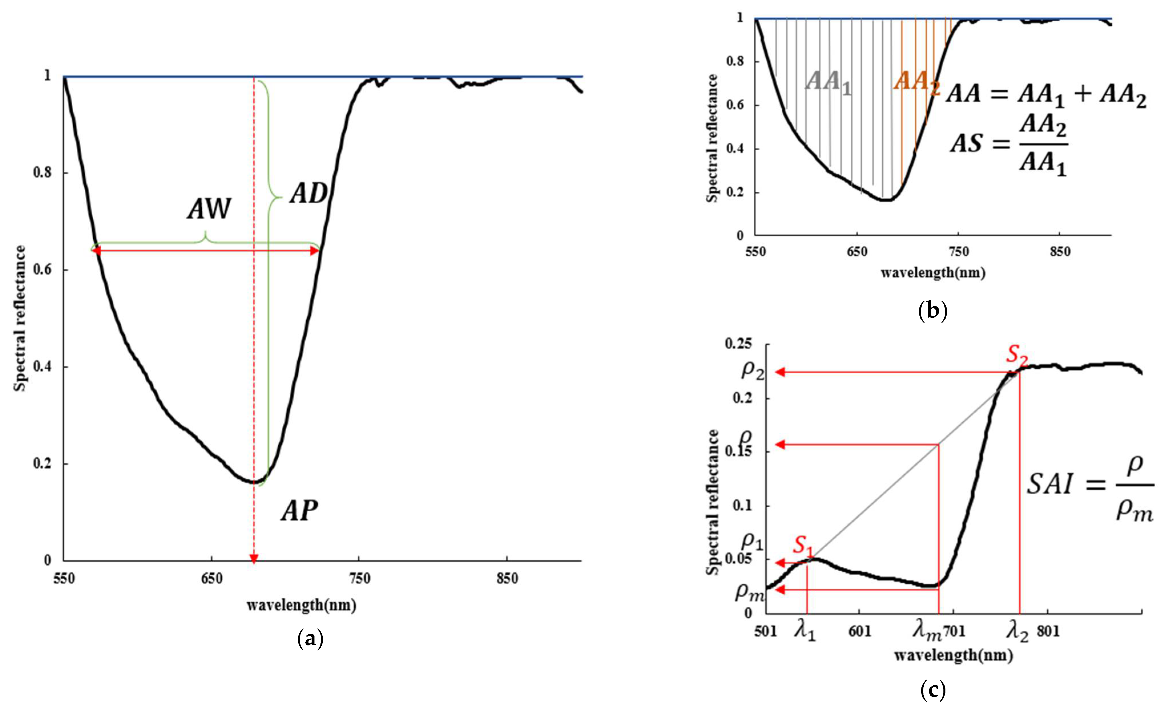
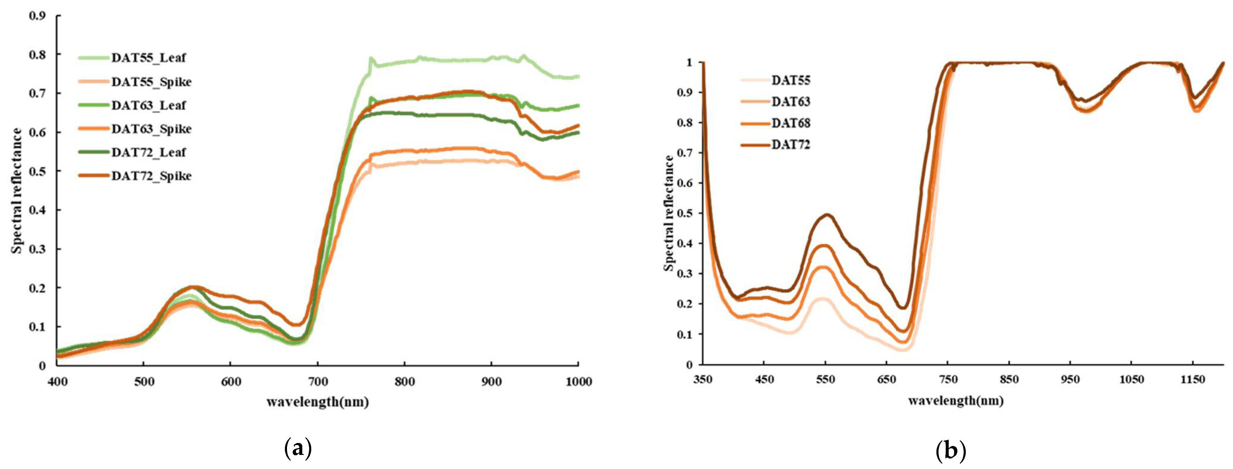
2.6.2. Spectral Absorption Characteristics Parameter

The spectral curve of the crop canopy collected by the ASD FieldSpec4 spectrometer can effectively reflect the absorption and reflection characteristics of the ground object. In the visible light band, due to the absorption effect of chlorophyll, there are two absorption peaks in the blue band and the red band. In the near-infrared band, due to the scattering effect of the canopy, a reflection platform with a relatively high reflectance is formed. The measurement is generally carried out from 10:00 to 14:00. Three positions are selected for each plot for measurement, and the measurement is repeated three times for each plot. The height of the spectrometer probe vertically downward from the top of the canopy is 0.7 to 1.0 m. To fully exploit the spectral information of the crop contained in the spectral curve, this study introduces the parameterization of spectral absorption characteristics into the estimation of crop growth parameters, fully considering the reflectance of multiple bands of the crop canopy and the waveform characteristics of the spectral curve.

Spectral absorption characteristics parameter quantifies the absorption peaks of the spectral curve into multiple spectral absorption characteristic parameters [67,68]. These spectral absorption characteristic parameters are used to locate the spectral absorption positions and quantify the shapes of absorption valleys. They include six parameters: absorption position (AP), absorption depth (AD), absorption width (AW), absorption area (AA), spectral absorption index (SAI), and absorption symmetry (AS). To extract the spectral absorption characteristic parameters, the spectral curve needs to be subjected to envelope line elimination first. The specific process of the envelope line algorithm is as follows: the first step is to find all the reflection rate maximum points of the spectral curve, and the second step is to find the envelope line points from the maximum point to the left and right, respectively. The envelope line points should satisfy the condition that the line segment formed by the previous envelope line point and the next envelope line point, and its subsequent extension line, are all above all the points after the previous envelope line point. Similarly, if the envelope line points are sought from the front, it is necessary to ensure that the line segment formed by the previous envelope line point and the next envelope line point and its subsequent extension line are all above all the points before the previous envelope line point.

AP: As shown in Figure 2a, the absorption position is the wavelength corresponding to the deepest absorption of the absorption valley after the envelope of the spectral curve is eliminated.

AD: As shown in Figure 2a, the absorption depth is the deepest absorption depth of the absorption valley after the envelope of the spectral curve is eliminated.

AW: As shown in Figure 2a, the absorption width is the spectral width at half of the maximum absorption depth in the absorption valley resulting from the elimination of the envelope of the spectral curve.

AA: As shown in Figure 2b, the spectral absorption area is the integral of the absorption depth of the absorption valley over the wavelength. If the spectrum is continuous, the absorption area equation is Equation (3).

$$\mathrm{A}\mathrm{A}={\int }_{{\mathsf{\lambda }}_1}^{{\mathsf{\lambda }}_2}\left(1-{\mathsf{\rho }}_{\mathsf{\lambda }}\right)\mathrm{d}\mathsf{\lambda }$$

(3)

If the spectrum is discrete, the absorption area equation is Equation (4).

$$\mathrm{A}\mathrm{A}=\sum _{\mathrm{i}=\mathrm{m}}^{\mathrm{n}}\left(1-{\mathsf{\rho }}_{\mathrm{i}}\right)$$

(4)

AS: As shown in Figure 2b, the vertical line of the absorption position is the boundary, and the ratio of the area of the right region to the area of the left region.

SAI: As shown in Figure 2c, the two shoulders S₁ and S₂ of the absorption valley of a spectral curve, and the lines between S₁ and S₂ are called the non-absorption baseline. The reflectivity ${\rho }_m$,$\rho$ is obtained from the spectral curve and non-absorption baselines S₁ and S₂, respectively. Equation (5) for calculating the spectral absorption index is as follows:

$$\mathrm{S}\mathrm{A}\mathrm{I}={\displaystyle \frac{\mathsf{\rho }}{{\mathsf{\rho }}_{\mathrm{m}}}}={\displaystyle \frac{\mathrm{d}·{\mathsf{\rho }}_2+\left(1-\mathrm{d}\right)·{\mathsf{\rho }}_1}{{\mathsf{\rho }}_{\mathrm{m}}}}$$

(5)

where d is the proportional parameter $\mathrm{d}=({\mathsf{\lambda }}_{\mathrm{m}}-{\mathsf{\lambda }}_1)/({\mathsf{\lambda }}_2-{\mathsf{\lambda }}_1)$.

The absorption of crops is mainly concentrated in the visible light band, so this experiment mainly extracted the absorption characteristic parameters of the visible light band absorption valley of the crop canopy. After envelope elimination in the crop canopy spectrum, there is a large absorption valley in the visible light band, which has two absorption bands, namely the blue band and the red band, and the absorption depth of the red band is usually greater than that of the blue band. If the two absorption bands of red and blue are taken as one absorption valley to extract the absorption feature, the absorption position of the absorption valley will be shifted to the red band, while the absorption position of the blue wave segment will be ignored. Moreover, the large absorption area of the blue wave segment will also affect the absorption area, absorption width, and absorption symmetry of the red band. In order to more accurately investigate the spectral absorption characteristic parameters of the two absorption bands, this study divided the large absorption valley in the visible light band into two absorption bands, red and blue, and extracted the absorption characteristic parameters of the two absorption bands, respectively, with the green band (550 nm) as the limit.

In the process of crop growth, the absorption of the blue band and red band will change to some extent. The absorption characteristic parameters of the two absorption bands can be used as the ratio or difference to reflect the absorption difference between the red and blue bands. Therefore, on the basis of extracting the absorption characteristics of the two absorption bands, the absorption characteristics of the two absorption bands are differentiated or compared, and the ratio of absorption characteristics parameters is proposed. The absorption characteristic parameters extracted from the hyperspectral data of crop canopy in this study are summarized in

Table 2. Spectral absorption characteristics parameter in this study.

Features	Description	Equation
RAA	Ratio absorption area	${\mathrm{A}\mathrm{A}}_{\mathrm{R}\mathrm{e}\mathrm{d}}/{\mathrm{A}\mathrm{A}}_{\mathrm{B}\mathrm{l}\mathrm{u}\mathrm{e}}$
RAW	Ratio absorption width	${\mathrm{A}\mathrm{W}}_{\mathrm{R}\mathrm{e}\mathrm{d}}/{\mathrm{A}\mathrm{W}}_{\mathrm{B}\mathrm{l}\mathrm{u}\mathrm{e}}$
RAD	Ratio absorption depth	${\mathrm{A}\mathrm{D}}_{\mathrm{R}\mathrm{e}\mathrm{d}}/{\mathrm{A}\mathrm{D}}_{\mathrm{B}\mathrm{l}\mathrm{u}\mathrm{e}}$
DSAI	Difference spectral absorption index	${(\mathrm{S}\mathrm{A}\mathrm{I}}_{\mathrm{R}\mathrm{e}\mathrm{d}}-{\mathrm{S}\mathrm{A}\mathrm{I}}_{\mathrm{B}\mathrm{l}\mathrm{u}\mathrm{e}})$
NDSAI	Normalized difference spectral absorption index	${(\mathrm{S}\mathrm{A}\mathrm{I}}_{\mathrm{R}\mathrm{e}\mathrm{d}}-{\mathrm{S}\mathrm{A}\mathrm{I}}_{\mathrm{B}\mathrm{l}\mathrm{u}\mathrm{e}})/{(\mathrm{S}\mathrm{A}\mathrm{I}}_{\mathrm{R}\mathrm{e}\mathrm{d}}+{\mathrm{S}\mathrm{A}\mathrm{I}}_{\mathrm{B}\mathrm{l}\mathrm{u}\mathrm{e}})$
RSAI	Ratio spectral absorption index	${\mathrm{S}\mathrm{A}\mathrm{I}}_{\mathrm{R}\mathrm{e}\mathrm{d}}/{\mathrm{S}\mathrm{A}\mathrm{I}}_{\mathrm{B}\mathrm{l}\mathrm{u}\mathrm{e}}$

.

2.6.3. Canopy Height

The RGB images of the study were used for canopy 3-D reconstruction. Using Pix4Dmapper, the canopy DSM was generated. The canopy height (H) was calculated as:

$$\mathrm{H}=\mathrm{D}\mathrm{S}\mathrm{M}-\mathrm{D}\mathrm{E}\mathrm{M}$$

(6)

where the $\mathrm{D}\mathrm{E}\mathrm{M}$ is equal to the DSM on the date before crop transplanting. This approach is widely applied to retrieve canopy height, with an accuracy of around 3 cm [69].

2.7. Analysis Methods

In this study, a tridimensional conceptual model of estimating maize AGB was proposed by combining the canopy height, VI, and spectral absorption characteristics parameters extracted from geometric data and multisource spectral data. Before crop heading, a linear function was constructed using the product of NDVI and the square of canopy height to estimate crop AGB. Due to the influence of spike dry weight on the estimation accuracy of crop AGB, the RSAI was introduced to characterize spike biomass on the basis of the original function, and the multiple linear regression model was used to estimate the total AGB. The accuracy of the AGB estimation model was evaluated by using the K-fold cross-validation method, where K was taken as 10. The main process is shown in Figure 3.

2.7.1. AGB Estimation Based on VI and Canopy Height

Many studies have shown that estimating AGB solely based on spectral data may lack the description of crop canopy structure [70,71], and combining spectral and geometric data can significantly improve the accuracy of AGB estimation [54,55,56]. In previous studies, some scholars used H × VI to estimate crop LAI and achieved good results [72], as shown in Equation (7). Some scholars also proposed a three-dimensional cube model to estimate maize AGB, in which AGB is the volume, LAI is the base area, canopy height is the height, and H × LAI is used to estimate crop AGB [57], as shown in Equation (8). Combined with the above studies, this study proposed H² × VI to estimate crop AGB, as shown in Equation (9).

$$\mathrm{L}\mathrm{A}\mathrm{I}\propto (\mathrm{V}\mathrm{I}\times \mathrm{H})$$

(7)

$$\mathrm{A}\mathrm{G}\mathrm{B}\propto (\mathrm{L}\mathrm{A}\mathrm{I}\times \mathrm{H})$$

(8)

$$\mathrm{A}\mathrm{G}\mathrm{B}\propto (\mathrm{V}\mathrm{I}\times {\mathrm{H}}^2)$$

(9)

2.7.2. Multiple Linear Regression

Multiple linear regression can fully consider a variety of features to participate in AGB estimation, and combine different features to build a regression model. Stepwise multiple linear regression on the basis of multiple linear regression, variables are introduced into the multiple linear regression model one by one. For each new variable introduced, the old variables of the selected model are tested one by one, and the variables that are considered meaningless and can be replaced are deleted. This method can effectively screen multiple features and build a linear regression model that integrates multiple features.

2.7.3. Random Forest Regression

The random forest regression algorithm is an ensemble learning algorithm based on decision trees. It combines the idea of random selection of set features and the ensemble idea, and is a combined classifier based on decision trees. Ensemble learning can incorporate multiple algorithms of different types or the same type. Random forest combines multiple algorithms of the same type to form a decision tree and establish a more powerful prediction model. In this study, due to the small number of features and sufficient sample size, and in order to avoid the model being overly complex, the max_depth was 15 and the n_estimators were 250. To avoid overfitting, the max_samples were 0.8, and regularization techniques were introduced during model training, with other model parameters set to default values.

2.7.4. Support Vector Regression

Support vector regression (abbreviated as SVR) is a regression analysis method based on support vector machine (SVM), and is widely used in the fields of prediction and pattern recognition. SVR achieves the prediction of continuous variables by finding an optimal hyperplane in a high-dimensional space to maximize the interval between data points and the hyperplane. This article will deeply explore the theoretical basis, mathematical principles, model construction, parameter selection, training and optimization, application scenarios of SVR, as well as its advantages and limitations. In this study, due to the small number of features and sufficient sample size, the kernel was ‘rbf’. Meanwhile, to avoid overfitting, the gamma was 1 and the C was 50, and other model parameters were set to default values.

3. Results

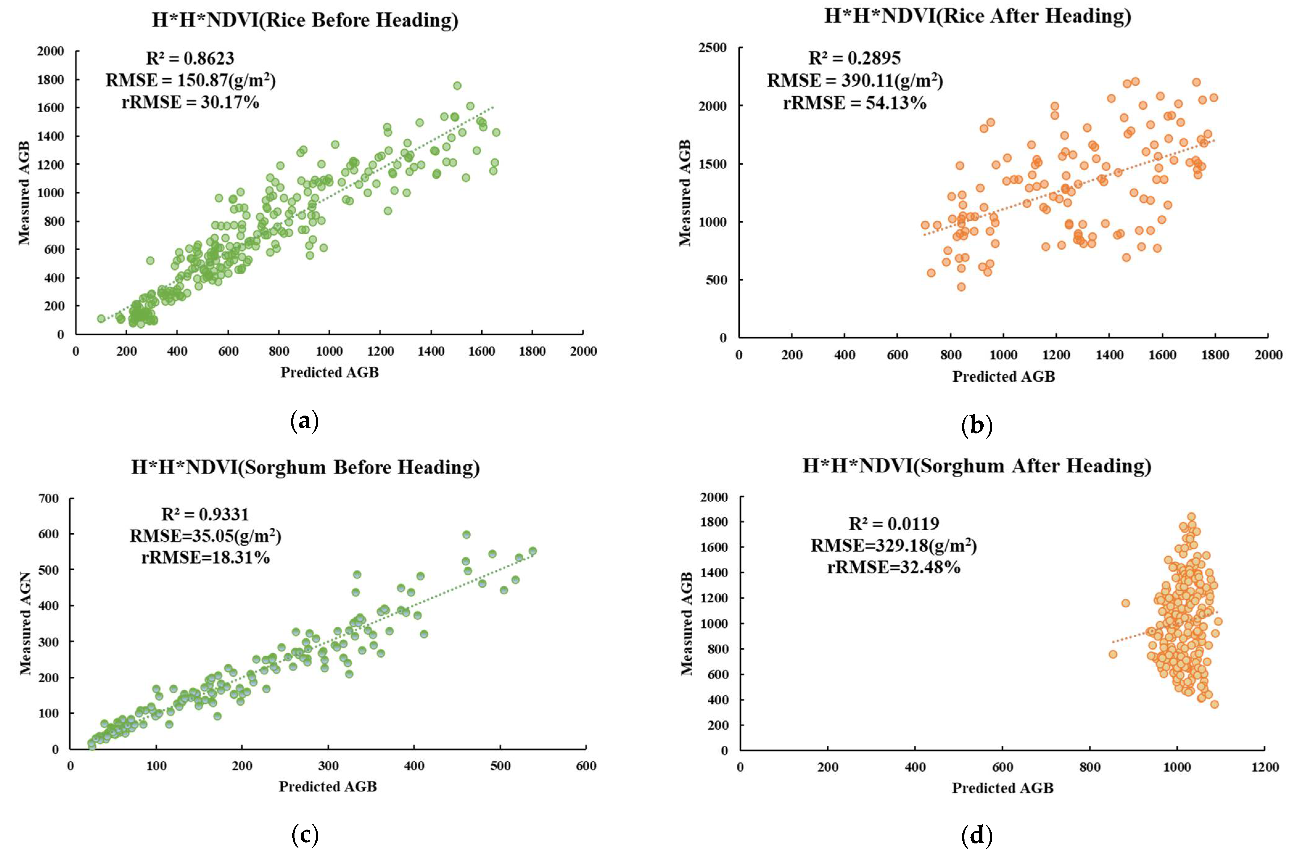
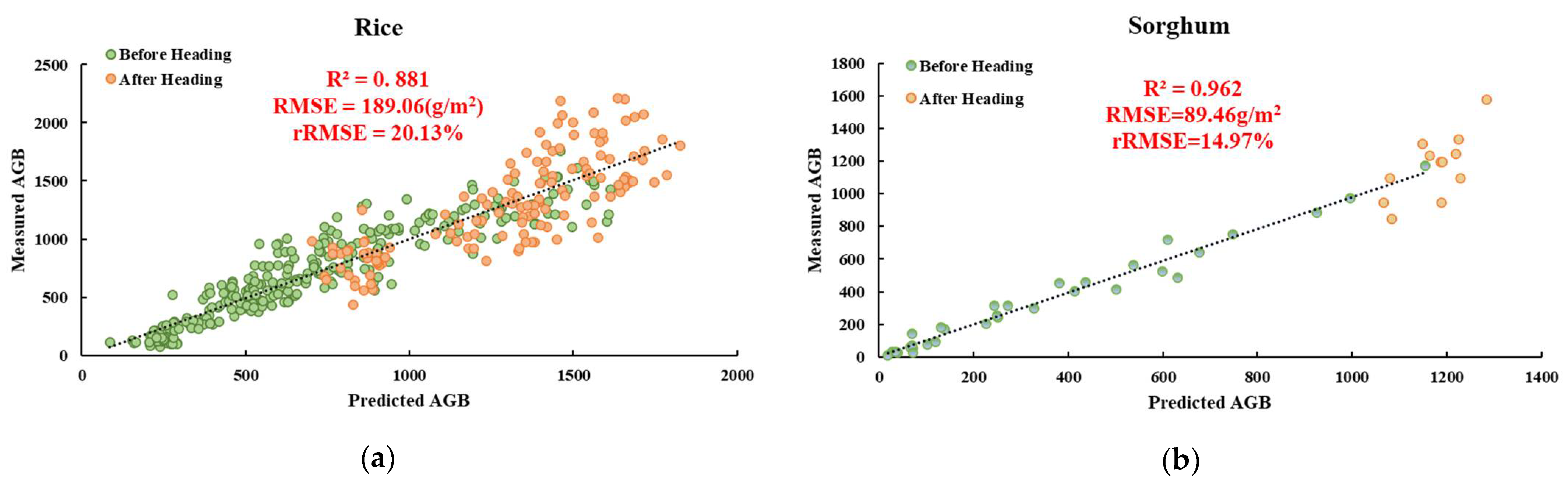
3.1. AGB Estimation Performance in Two Stages

In this study, the H² × VI model was used to estimate crop AGB. NDVI, NDRE, EVI2, and OSAVI were selected by VI, and the model was divided into two parts: before heading and after heading. The results are shown in

Table 3. Rice AGB estimation results based on H² × VI before heading and after heading.

Model	Stage	R2	RMSE (g/m2)	rRMSE (%)
H2 × NDVI	Before heading	0.86	150.87	30.17
	After heading	0.26	390.11	54.13
H2 × EVI2	Before heading	0.82	177.71	35.54
	After heading	0.32	388.82	53.98
H2 × NDRE	Before heading	0.83	187.40	37.48
	After heading	0.15	467.73	62.90
H2 × OSAVI	Before heading	0.85	155.47	31.10
	After heading	0.21	407.65	56.12

and

Table 4. Sorghum AGB estimation results based on H² × VI before heading and after heading.

Model	Stage	R2	RMSE (g/m2)	rRMSE(%)
H2 × NDVI	Before heading	0.93	35.05	18.31
	After heading	0.01	329.18	36.45
H2 × EVI2	Before heading	0.93	75.86	39.64
	After heading	0.07	320.02	35.57
H2 × NDRE	Before heading	0.92	37.37	19.53
	After heading	0.09	315.93	34.17
H2 × OSAVI	Before heading	0.92	37.29	19.49
	After heading	0.11	313.15	33.89

and Figure 4.

According to the above results, the model has a good effect on estimating crop AGB before heading, but a poor effect after heading, especially for sorghum. Therefore, it is necessary to improve the after-heading model to improve the accuracy of AGB estimation.

From the perspective of crop canopy spectrum, the canopy spectrum before heading was composed of the interaction between stem spectrum and leaf spectrum, and the effect of spike spectrum was increased after heading, as shown in Figure 5. From the perspective of crop growth law, the AGB before heading only consisted of stem and leaf biomass, while the spike biomass increased after heading, as shown in Figure 6 for rice.

We speculated that the model’s accuracy was reduced due to the influence of spike biomass, so we separately analyzed the correlation between H² × VI and stem and leaf biomass and spike biomass after heading. The results are shown in

Table 5. R² between H² × VI AGB in different parts after heading.

Features	R2 (AGB_Leaf+Stem)	R2 (AGB_Spike)
H2 × NDVI	0.5587	0.0034
H2 × EVI2	0.5663	0.0151
H2 × NDRE	0.5517	0.0749
H2 × OSAVI	0.5078	0.0019

.

It can be seen from the results of Table 4 that H² × VI has a strong correlation with stem and leaf biomass after heading, but has almost no correlation with spike biomass. Therefore, to estimate the crop AGB model, it is necessary to introduce features that have a strong correlation with spike biomass to characterize spike biomass after heading, so as to improve the estimation accuracy of the model.

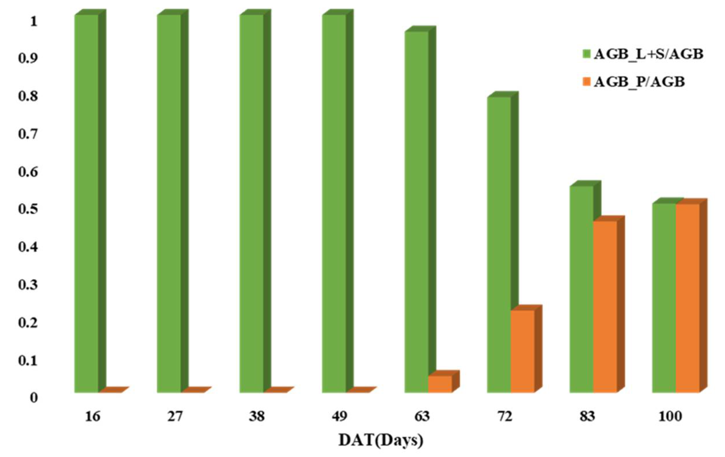
3.2. Adding Spectral Absorption Characteristic Parameter After Heading

In order to find the features related to spike biomass, we separately measured the end element spectra of leaves and spikes, and found that the reflectance of spikes gradually increased with time in the red band and blue wave segment, as shown in Figure 7a. Compared with the leaf spectrum, the absorption valley in the red band was more different in different stages after heading, which suggested that the absorption characteristics of the spectrum in the red band had a certain correlation with spike biomass.

After heading, the canopy reflectance of the crop in the visible band increased slowly with the growth of the crop. There was an absorption valley in the red and blue bands, and a reflection peak in the green band. Reflection decreased first and then increased in the near infrared band, which was inconsistent with the change law of spike biomass. Moreover, the reflection peak in the green band was mainly caused by leaf reflection. Therefore, the reflectance of red and blue wave segments is selected as the research object, and the difference degree of features in different stages is increased by envelope removal. Finally, the characteristics of the absorption valley of red and blue wave segments are extracted by spectral feature quantization.

After envelope elimination, the reflectance of the canopy spectral curve after crop heading had a large difference in the red band and a small difference in the blue band, as shown in Figure 7b. The spectral absorption features of the two bands were extracted, and the differences in the characteristic values in different stages were increased by ratio, difference, and normalization operations.

Correlation analysis was conducted between the new characteristics obtained by the above calculation and spike biomass. The results are shown in

Table 6. R² between spectral absorption characteristic parameter and spike AGB after heading.

Features	R2 (AGB_Spike)
RAA	0.2059
RAW	0.1688
RAD	0.2649
DSAI	0.0624
NDSAI	0.5363
RSAI	0.6152

, in which the RSAI had the highest correlation with spike biomass and a strong correlation. Therefore, we used the RSAI to characterize spike biomass.

H² × NDVI, which had the highest correlation with stem and leaf biomass, and RSAI, which had the highest correlation with spike biomass, were selected as the input features of the model to construct the after-heading AGB estimation model, and the regression effects of random forest regression, support vector machine regression, and multiple linear regression models were tested. Finally, the K-fold crossover model was used to verify the results to ensure they were statistically significant. The results are shown in

Table 7. R² and RMSE of AGB estimation based on H² × VI and spectral absorption characteristic parameter after heading.

Model	R2 (Training Set)	RMSE (g/m2) (Training Set)	R2 (Test Set)	RMSE (g/m2) (Test Set)
Random Forest Regression	0.93	201.34	0.82	269.56
Support Vector Regression	0.78	392.91	0.78	394.70
Multiple Linear Regression	0.89	260.58	0.89	262.86

.

Among the three models, we selected the multiple linear regression model with the highest test set accuracy to estimate the rice AGB after heading, and we used the linear regression model of H² × NDVI before heading. The model equations are shown in

Table 8. AGB estimation model expressions.

Crop	Stage	Model
Rice	Before heading	AGB = 1412.1 × H2 × NDVI + 75.93
Rice	After heading	AGB = 931.26 × H2 × NDVI − 595.08 × RSAI + 1845.64
Sorghum	Before heading	AGB = 113.46 × H2 × NDVI + 9.01
Sorghum	After heading	AGB = 59.921 × H2 × NDVI − 343.5 × RSAI + 1488.08

, and the final result is shown in Figure 8.

4. Discussion

Before heading, the vegetative growth of the crop was the main factor, and the height of the canopy gradually increased. At the same time, the AGB of the crop was mainly increased by stem and leaf biomass, and the increase in stem and leaf biomass was mainly related to chlorophyll. With the increase in chlorophyll content, the reflectance of the canopy gradually increased in the near-infrared band, while the reflectance in the green band gradually decreased. At the same time, NDVI and other VIs can well reflect the change of chlorophyll content, so the product of VI and the square of canopy height can be used to estimate crop AGB, as shown in Table 3 and Table 4 and Figure 4.

However, after crop heading, the crop mainly grows by reproduction, and the AGB is composed of stem, leaf, and spike biomass, and the canopy height basically does not change. As can be seen from Figure 5 and Figure 6, the increase in AGB was dominated by spike biomass, while the stem and leaf biomass increased slowly, and spike biomass accounted for an increasing proportion of AGB. The increase in spike biomass was mainly related to carotenoids, so the effect of estimating AGB by H² × VI decreased significantly, as shown in Table 3 and Table 4 and Figure 4.

As can be seen from Figure 7, with the decrease in carotenoid content, the absorption of the red and blue bands gradually decreases, and the canopy reflectance in these two bands gradually increases. Then, the difference of canopy reflectance in different stages is eliminated and increased through the envelope. Because the increase in reflectance in the red band is smaller than that in the blue band, the change in the RSAI is exactly the same as that of carotenoid. Therefore, the introduction of the RSAI on the basis of the product of the original VI and the square of the canopy height can effectively estimate crop AGB after heading, as shown in Table 6.

As can be seen from Table 7, the support vector machine regression model has the worst effect. Although the random forest model has a good effect on the training set, its effect on the test set is not as good as that of the multiple linear regression model. Moreover, the multiple linear regression model has a simple structure and few parameters, so we adopt the multiple linear regression model.

The effect of the constructed multiple linear regression model (H² × NDVI, RSAI) in estimating AGB after heading was significantly improved compared with NDVI, H² × NDVI, and RSAI, as shown in

Table 9. R² and RMSE of AGB estimation based on different characteristics after heading.

Model	R2 (Training Set)	RMSE (g/m2) (Training Set)	R2 (Test Set)	RMSE (g/m2) (Test Set)
NDVI	0.08	455.80	0.04	461.47
H2 × NDVI	0.53	390.11	0.51	391.91
RSAI	0.72	307.89	0.70	309.76
Multiple Linear Regression (H2 × NDVI, RSAI)	0.89	260.58	0.89	262.86

.

The linear regression model of H² × NDVI was used before heading, and the multiple linear regression models of H² × NDVI and RSAI were used to estimate AGB in different stages after heading. Compared with the model that directly estimates AGB throughout the entire growth period using H² × VI, the effect of our model was significantly improved. The test set results of K-fold cross-validation are shown in

Table 10. Rice AGB estimation results (the test set results of K-fold cross-validation) based on different characteristics throughout the entire growth period.

Model	R2	RMSE (g/m2)	rRMSE (%)
H2 × NDVI	0.65	294.68	35.32
H2 × EVI2	0.64	298.60	36.67
H2 × NDRE	0.63	306.76	37.48
H2 × OSAVI	0.63	298.21	36.62
f(H2 × NDVI, RSAI)	0.88	189.06	20.13

and

Table 11. Sorghum AGB estimation results (the test set results of K-fold cross-validation) based on different characteristics throughout the entire growth period.

Model	R2	RMSE (g/m2)	rRMSE (%)
H2 × NDVI	0.63	296.49	42.68
H2 × EVI2	0.48	357.28	51.43
H2 × NDRE	0.44	367.89	52.95
H2 × OSAVI	0.41	379.10	54.57
f(H2 × NDVI, RSAI)	0.96	89.46	14.97

.

Xu et al. constructed a multiple linear regression model using the texture features and spectral features in the hyperspectral images of UAV to estimate rice AGB, with R² = 0.76, and rRMSE = 27.10% [1]. Tunca et al. used high-resolution UAV data and machine learning (ML) to estimate sorghum AGB, with R² = 0.80, and RMSE = 290 g/m² [73]. Compared with previous studies, our method has achieved partial improvement in estimating rice AGB and significant improvement in estimating sorghum AGB.

As can be seen from Figure 8, although the estimation effect of crop AGB after heading is significantly improved, the accuracy of estimating rice AGB in the later stage still decreases. This is due to the influence of spike weight, which leads to a reduction in canopy height and thus a decline in the accuracy of estimating stem and leaf biomass by H² × VI. One of the reasons why the AGB estimation of sorghum is significantly better than that of rice is due to the small amount of sorghum data, and another reason is that the spike of sorghum changes from green to red, and the absorption in the red band changes more obviously than that of rice, so RSAI is more sensitive to the change of spike biomass. In subsequent studies, we will consider replacing the canopy height with the variation of the canopy height in two adjacent periods to improve the accuracy of AGB estimation. Meanwhile, our method may also be extended and applied to satellite remote sensing in the future to improve the accuracy of large-scale crop AGB estimation.

5. Conclusions

In this study, aiming to address the problem that the accuracy of H² × VI estimation of crop AGB after heading is greatly reduced, we introduced the spectral absorption characteristic parameter RSAI, which is consistent with the change of spike biomass, from the perspective of the spectral variation rule of crop canopy after heading, and used it to characterize spike biomass. Together with H² × VI, we constructed a multiple linear regression model to estimate crop AGB after heading. Compared with only using H² × VI, the accuracy is effectively improved, the R² of the entire growth period was increased to 0.88, and the rRMSE was reduced by 15% in rice; the R² of the entire growth period was increased to 0.96, and the rRMSE was reduced by 27% in sorghum.

This study provided an accurate AGB estimation model throughout the entire growth period for crops with conspicuous spikes, which effectively improved the estimation accuracy in the reproductive stage and provided reliable information for evaluating crop growth at the plot scale.

References

1. Xu, T.Y.; Wang, F.M.; Xie, L.L.; Yao, X.P.; Zheng, J.Y.; Li, J.L.; Chen, S.T. Integrating the Textural and Spectral Information of UAV Hyperspectral Images for the Improved Estimation of Rice Aboveground Biomass. Remote Sens. 2022, 14, 2534. [Google Scholar] [CrossRef]
2. Chen, Z.X.; Ren, J.Q.; Tang, H.J.; Shi, Y.; Len, P.; Liu, J.; Wang, L.M.; Wu, W.B.; Yao, Y.M.; Hasituya. Progress and prospect of agricultural remote sensing research and application. J. Remote Sens. 2016, 20, 748–767. [Google Scholar]
3. Yang, S.X.; Feng, Q.S.; Liang, T.G.; Liu, B.K.; Zhang, W.J.; Xie, H.J. Modeling grassland above-ground biomass based on artificial neural network and remote sensing in the Three-River Headwaters Region. Remote Sens. Environ. 2018, 204, 448–455. [Google Scholar] [CrossRef]
4. Yu, Y.; Pan, Y.; Yang, X.; Fan, W. Spatial Scale Effect and Correction of Forest Aboveground Biomass Estimation Using Remote Sensing. Remote Sens. 2022, 14, 2828. [Google Scholar] [CrossRef]
5. Liu, Y.; Feng, H.; Yue, J.; Li, Z.; Jin, X.; Fan, Y.; Feng, Z.; Yang, G. Estimation of Aboveground Biomass of Potatoes Based on Characteristic Variables Extracted from UAV Hyperspectral Imagery. Remote Sens. 2022, 14, 5121. [Google Scholar] [CrossRef]
6. Wocher, M.; Berger, K.; Verrelst, J.; Hank, T. Retrieval of carbon content and biomass from hyperspectral imagery over cultivated areas. ISPRS J. Photogramm. Remote Sens. 2022, 193, 104–114. [Google Scholar] [CrossRef] [PubMed]
7. Musthafa, M.; Singh, G. Improving Forest Above-Ground Biomass Retrieval Using Multi-Sensor L- and C- Band SAR Data and Multi-Temporal Spaceborne LiDAR Data. Front. For. Glob. Chang. 2022, 5, 822704. [Google Scholar] [CrossRef]
8. Santoro, M.; Cartus, O.; Wegmüller, U.; Besnard, S.; Carvalhais, N.; Araza, A.; Herold, M.; Liang, J.; Cavlovic, J.; Engdahl, M.E. Global estimation of above-ground biomass from spaceborne C-band scatterometer observations aided by LiDAR metrics of vegetation structure. Remote Sens. Environ. 2022, 279, 113114. [Google Scholar] [CrossRef]
9. Quan, X.W.; He, B.B.; Yebra, M.; Yin, C.M.; Liao, Z.M.; Zhang, X.T.; Li, X. A radiative transfer model-based method for the estimation of grassland aboveground biomass. Int. J. Appl. Earth Obs. Geoinf. 2017, 54, 159–168. [Google Scholar] [CrossRef]
10. Rotter, R.P.; Palosuo, T.; Kersebaum, K.C.; Angulo, C.; Bindi, M.; Ewert, F.; Ferrise, R.; Hlavinka, P.; Moriondo, M.; Nendel, C.; et al. Simulation of spring barley yield in different climatic zones of Northern and Central Europe: A comparison of nine crop models. Field Crops Res. 2012, 133, 23–36. [Google Scholar] [CrossRef]
11. Kaur, S.; Singh, M. Modeling the crop growth—A review. Mausam 2020, 71, 103–114. [Google Scholar]
12. Yuan, W.P.; Cai, W.W.; Xia, J.Z.; Chen, J.Q.; Liu, S.G.; Dong, W.J.; Merbold, L.; Law, B.; Arain, A.; Beringer, J.; et al. Global comparison of light use efficiency models for simulating terrestrial vegetation gross primary production based on the La Thuile database. Agric. For. Meteorol. 2014, 192, 108–120. [Google Scholar] [CrossRef]
13. Zhang, L.; Gao, H.; Zhang, X. Combining Radiative Transfer Model and Regression Algorithms for Estimating Aboveground Biomass of Grassland in West Ujimqin, China. Remote Sens. 2023, 15, 2918. [Google Scholar] [CrossRef]
14. Cheng, Z.Q.; Meng, J.H.; Jiang, J.F.; Wang, Y.; Fang, H.T.; Yu, L.H. Estimation of above-ground biomass of maize in late growing period based on WOFOST model and UAV data. J. Remote. Sens. 2020, 24, 1403–1418. [Google Scholar]
15. Jones, J.W.; Hoogenboom, G.; Porter, C.H.; Boote, K.J.; Batchelor, W.D.; Hunt, L.A.; Wilkens, P.W.; Singh, U.; Gijsman, A.J.; Ritchie, J.T. The DSSAT cropping system model. Eur. J. Agron. 2003, 18, 235–265. [Google Scholar] [CrossRef]
16. Lara, M.A.S.; Pedreira, C.G.S.; Boote, K.J.; Pedreira, B.C.; Moreno, L.S.B.; Alderman, P.D. Predicting Growth of Panicum maximum: An Adaptation of the CROPGRO-Perennial Forage Model. Agron. J. 2012, 104, 600–611. [Google Scholar] [CrossRef]
17. Pedreira, B.C.; Pedreira, C.G.S.; Boote, K.J.; Lara, M.A.S.; Alderman, P.D. Adapting the CROPGRO perennial forage model to predict growth of Brachiaria brizantha. Field Crops Res. 2011, 120, 370–379. [Google Scholar] [CrossRef]
18. Pequeno, D.N.L.; Pedreira, C.G.S.; Boote, K.J. Simulating forage production of Marandu palisade grass (Brachiaria brizantha) with the CROPGRO-Perennial Forage model. Crop Pasture Sci. 2014, 65, 1335–1348. [Google Scholar] [CrossRef]
19. Sau, F.; Boote, K.J.; Bostick, W.M.; Jones, J.W.; Minguez, M.I. Testing and improving evapotranspiration and soil water balance of the DSSAT crop models. Agron. J. 2004, 96, 1243–1257. [Google Scholar] [CrossRef]
20. Chen, J.S.; Huang, J.X.; Lin, H.; Pei, Z.Y. Rice yield estimation method based on remote sensing information and crop growth model assimilation. Sci. China Inf. Sci. 2010, 40, 173–183. [Google Scholar]
21. de Wit, A.; Boogaard, H.; Fumagalli, D.; Janssen, S.; Knapen, R.; van Kraalingen, D.; Supit, I.; van der Wijngaart, R.; van Diepen, K. 25 years of the WOFOST cropping systems model. Agric. Syst. 2019, 168, 154–167. [Google Scholar] [CrossRef]
22. Zhuo, W.; Fang, S.; Gao, X.; Wang, L.; Wu, D.; Fu, S.; Wu, Q.; Huang, J. Crop yield prediction using MODIS LAI, TIGGE weather forecasts and WOFOST model: A case study for winter wheat in Hebei, China during 2009–2013. Int. J. Appl. Earth Obs. Geoinf. 2022, 106, 102668. [Google Scholar] [CrossRef]
23. Holzworth, D.P.; Huth, N.I.; Devoil, P.G.; Zurcher, E.J.; Herrmann, N.I.; McLean, G.; Chenu, K.; van Oosterom, E.J.; Snow, V.; Murphy, C.; et al. APSIM—Evolution towards a new generation of agricultural systems simulation. Environ. Model. Softw. 2014, 62, 327–350. [Google Scholar] [CrossRef]
24. Asseng, S.; Keating, B.A.; Fillery, I.R.P.; Gregory, P.J.; Bowden, J.W.; Turner, N.C.; Palta, J.A.; Abrecht, D.G. Performance of the APSIM-wheat model in Western Australia. Field Crops Res. 1998, 57, 163–179. [Google Scholar] [CrossRef]
25. Asseng, S.; van Keulen, H.; Stol, W. Performance and application of the APSIM Nwheat model in the Netherlands. Eur. J. Agron. 2000, 12, 37–54. [Google Scholar] [CrossRef]
26. Keating, B.A.; Carberry, P.S.; Hammer, G.L.; Probert, M.E.; Robertson, M.J.; Holzworth, D.; Huth, N.I.; Hargreaves, J.N.G.; Meinke, H.; Hochman, Z.; et al. An overview of APSIM, a model designed for farming systems simulation. Eur. J. Agron. 2003, 18, 267–288. [Google Scholar] [CrossRef]
27. Potter, C.S.; Randerson, J.T.; Field, C.B.; Matson, P.A.; Klooster, S.A. Terrestrial Ecosystem Production: A Process Model Based on Global Satellite and Surface Data. Glob. Biogeochem. Cycles 1993, 7, 811–841. [Google Scholar] [CrossRef]
28. Raza, S.M.H.; Mahmood, S.A. Estimation of Net Rice Production through Improved CASA Model by Addition of Soil Suitability Constant ((h)over-bar alpha). Sustainability 2018, 10, 1788. [Google Scholar] [CrossRef]
29. Liu, Z.Z.; Zhang, X.W.; Chen, Y.S.; Zhang, C.C.; Qin, F.; Zeng, H.W. Remote sensing estimation of regional winter wheat biomass based on CASA mode. Trans. Agric. Eng. 2017, 33, 225–233+315–316. [Google Scholar]
30. Zhao, Y.; Mao, D.; Zhang, D.; Wang, Z.; Du, B.; Yan, H.; Qiu, Z.; Feng, K.; Wang, J.; Jia, M. Mapping Phragmites australis Aboveground Biomass in the Momoge Wetland Ramsar Site Based on Sentinel-1/2 Images. Remote Sens. 2022, 14, 694. [Google Scholar] [CrossRef]
31. Goetz, S.J.; Prince, S.D.; Goward, S.N.; Thawley, M.M.; Small, J. Satellite remote sensing of primary production: An improved production efficiency modeling approach. Ecol. Model. 1999, 122, 239–255. [Google Scholar] [CrossRef]
32. Darvishzadeh, R.; Skidmore, A.; Schlerf, M.; Atzberger, C. Inversion of a radiative transfer model for estimating vegetation LAI and chlorophyll in a heterogeneous grassland. Remote Sens. Environ. 2008, 112, 2592–2604. [Google Scholar] [CrossRef]
33. Adeluyi, O.; Harris, A.; Verrelst, J.; Foster, T.; Claya, G.D. Estimating the phenological dynamics of irrigated rice leaf area index using the combination of PROSAIL and Gaussian Process Regression. Int. J. Appl. Earth Obs. Geoinf. 2021, 102, 102454. [Google Scholar] [CrossRef] [PubMed]
34. Wang, Z.; He, L.; He, Z.; Wang, X.; Li, L.; Kang, G.; Bai, W.; Chen, X.; Zhao, Y.; Xiao, Y. Integrating the PROSAIL and SVR Models to Facilitate the Inversion of Grassland Aboveground Biomass: A Case Study of Zoigê Plateau, China. Remote Sens. 2024, 16, 1117. [Google Scholar] [CrossRef]
35. Elshikha, D.E.M.; Hunsaker, D.J.; Waller, P.M.; Thorp, K.R.; Dierig, D.; Wang, G.; Cruz, V.M.V.; Katterman, M.E.; Bronson, K.F.; Wall, G.W.; et al. Estimation of direct-seeded guayule cover, crop coefficient, and yield using UAS-based multispectral and RGB data. Agric. Water Manag. 2022, 265, 107540. [Google Scholar] [CrossRef]
36. Li, B.; Xu, X.; Zhang, L.; Han, J.; Bian, C.; Li, G.; Liu, J.; Jin, L. Above-ground biomass estimation and yield prediction in potato by using UAV-based RGB and hyperspectral imaging. ISPRS J. Photogramm. Remote Sens. 2020, 162, 161–172. [Google Scholar] [CrossRef]
37. Yue, J.; Yang, G.; Tian, Q.; Feng, H.; Xu, K.; Zhou, C. Estimate of winter-wheat above-ground biomass based on UAV ultrahigh-ground-resolution image textures and vegetation indices. ISPRS J. Photogramm. Remote Sens. 2019, 150, 226–244. [Google Scholar] [CrossRef]
38. Luo, S.; Jiang, X.; He, Y.; Li, J.; Jiao, W.; Zhang, S.; Xu, F.; Han, Z.; Sun, J.; Yang, J.; et al. Multi-dimensional variables and feature parameter selection for aboveground biomass estimation of potato based on UAV multispectral imagery. Front. Plant Sci. 2022, 13, 948249. [Google Scholar] [CrossRef]
39. Xu, L.; Zhou, L.; Meng, R.; Zhao, F.; Lv, Z.; Xu, B.; Zeng, L.; Yu, X.; Peng, S. An improved approach to estimate ratoon rice aboveground biomass by integrating UAV-based spectral, textural and structural features. Precis. Agric. 2022, 23, 1276–1301. [Google Scholar] [CrossRef]
40. Chen, P.F.; Wang, J.L.; Liao, X.Y.; Yin, F.; Chen, B.R.; Liu, R. Inversion of above-ground biomass of grassland in Hulunbuir based on remote sensing data from environmental disaster reduction satellites. J. Nat. Resour. 2010, 25, 1122–1131. [Google Scholar]
41. Bao, Y.; Wei, G.; Gao, Z. Estimation of winter wheat biomass based on remote sensing data at various spatial and spectral resolutions. Front. Earth Sci. China 2009, 3, 118–128. [Google Scholar] [CrossRef]
42. Mutanga, O.; Skidmore, A.K. Narrow band vegetation indices overcome the saturation problem in biomass estimation. Int. J. Remote Sens. 2004, 25, 3999–4014. [Google Scholar] [CrossRef]
43. Fu, Y.Y.; Yang, G.J.; Wang, J.H.; Song, X.Y.; Feng, H.K. Winter wheat biomass estimation based on spectral indices, band depth analysis and partial least squares regression using hyperspectral measurements. Comput. Electron. Agric. 2014, 100, 51–59. [Google Scholar] [CrossRef]
44. Thenkabail, P.S.; Smith, R.B.; De Pauw, E. Hyperspectral vegetation indices and their relationships with agricultural crop characteristics. Remote Sens. Environ. 2000, 71, 158–182. [Google Scholar] [CrossRef]
45. Feng, H.; Fan, Y.; Yue, J.; Bian, M.; Liu, Y.; Chen, R.; Ma, Y.; Fan, J.; Yang, G.; Zhao, C. Estimation of potato above-ground biomass based on the VGC-AGB model and deep learning. Comput. Electron. Agric. 2025, 232, 110122. [Google Scholar] [CrossRef]
46. Duan, B.; Liu, Y.; Gong, Y.; Peng, Y.; Wu, X.; Zhu, R.; Fang, S. Remote estimation of rice LAI based on Fourier spectrum texture from UAV image. Plant Methods 2019, 15, 124. [Google Scholar] [CrossRef] [PubMed]
47. Freitas, R.G.; Pereira, F.R.S.; Dos Reis, A.A.; Magalhães, P.S.G.; Figueiredo, G.K.D.A.; do Amaral, L.R. Estimating pasture aboveground biomass under an integrated crop-livestock system based on spectral and texture measures derived from UAV images. Comput. Electron. Agric. 2022, 198, 107122. [Google Scholar] [CrossRef]
48. Lu, D.; Batistella, M. Exploring TM image texture and its relationships with biomass estimation in Rondônia, Brazilian Amazon. Acta Amaz. 2005, 35, 249–257. [Google Scholar] [CrossRef]
49. Nichol, J.E.; Sarker, M.L.R. Improved Biomass Estimation Using the Texture Parameters of Two High-Resolution Optical Sensors. IEEE Trans. Geosci. Remote Sens. 2011, 49, 930–948. [Google Scholar] [CrossRef]
50. Fu, Y.Y.; Yang, G.J.; Li, Z.H.; Song, X.Y.; Li, Z.H.; Xu, X.G.; Wang, P.; Zhao, C.J. Winter Wheat Nitrogen Status Estimation Using UAV-Based RGB Imagery and Gaussian Processes Regression. Remote Sens. 2020, 12, 3778. [Google Scholar] [CrossRef]
51. Fu, Y.Y.; Yang, G.J.; Song, X.Y.; Li, Z.H.; Xu, X.G.; Feng, H.K.; Zhao, C.J. Improved Estimation of Winter Wheat Aboveground Biomass Using Multiscale Textures Extracted from UAV-Based Digital Images and Hyperspectral Feature Analysis. Remote Sens. 2021, 13, 581. [Google Scholar] [CrossRef]
52. Liu, J.; Zhu, Y.; Song, L.; Su, X.; Li, J.; Zheng, J.; Zhu, X.; Ren, L.; Wang, W.; Li, X. Optimizing window size and directional parameters of GLCM texture features for estimating rice AGB based on UAVs multispectral imagery. Front. Plant Sci. 2023, 14, 1284235. [Google Scholar] [CrossRef]
53. Jimenez-Berni, J.A.; Deery, D.M.; Rozas-Larraondo, P.; Condon, A.G.; Rebetzke, G.J.; James, R.A.; Bovill, W.D.; Furbank, R.T.; Sirault, X.R.R. High Throughput Determination of Plant Height, Ground Cover, and Above-Ground Biomass in Wheat with LiDAR. Front. Plant Sci. 2018, 9, 237. [Google Scholar] [CrossRef] [PubMed]
54. Tilly, N.; Aasen, H.; Bareth, G. Fusion of Plant Height and Vegetation Indices for the Estimation of Barley Biomass. Remote Sens. 2015, 7, 11449–11480. [Google Scholar] [CrossRef]
55. Yue, J.B.; Feng, H.K.; Jin, X.L.; Yuan, H.H.; Li, Z.H.; Zhou, C.Q.; Yang, G.J.; Tian, Q.J. A Comparison of Crop Parameters Estimation Using Images from UAV-Mounted Snapshot Hyperspectral Sensor and High-Definition Digital Camera. Remote Sens. 2018, 10, 1138. [Google Scholar] [CrossRef]
56. Navarro, J.A.; Algeet, N.; Fernandez-Landa, A.; Esteban, J.; Rodriguez-Noriega, P.; Guillen-Climent, M.L. Integration of UAV, Sentinel-1, and Sentinel-2 Data for Mangrove Plantation Aboveground Biomass Monitoring in Senegal. Remote Sens. 2019, 11, 77. [Google Scholar] [CrossRef]
57. Meiyan, S.; Mengyuan, S.; Qizhou, D.; Xiaohong, Y.; Baoguo, L.; Yuntao, M. Estimating the maize above-ground biomass by constructing the tridimensional concept model based on UAV-based digital and multi-spectral images. Field Crops Res. 2022, 282, 108491. [Google Scholar] [CrossRef]
58. Liu, Y.; Feng, H.; Yue, J.; Jin, X.; Fan, Y.; Chen, R.; Bian, M.; Ma, Y.; Li, J.; Xu, B.; et al. Improving potato AGB estimation to mitigate phenological stage impacts through depth features from hyperspectral data. Comput. Electron. Agric. 2024, 219, 108808. [Google Scholar] [CrossRef]
59. Liu, Y.; Feng, H.; Yue, J.; Jin, X.; Fan, Y.; Chen, R.; Bian, M.; Ma, Y.; Song, X.; Yang, G. Improved potato AGB estimates based on UAV RGB and hyperspectral images. Comput. Electron. Agric. 2023, 214, 108260. [Google Scholar] [CrossRef]
60. Liu, T.; Wang, J.; Wang, J.; Zhao, Y.; Wang, H.; Zhang, W.; Yao, Z.; Liu, S.; Zhong, X.; Sun, C. Research on the estimation of wheat AGB at the entire growth stage based on improved convolutional features. J. Integr. Agric. 2025, 24, 1403–1423. [Google Scholar] [CrossRef]
61. Gnyp, M.L.; Miao, Y.; Yuan, F.; Ustin, S.L.; Yu, K.; Yao, Y.; Huang, S.; Bareth, G. Hyperspectral canopy sensing of paddy rice aboveground biomass at different growth stages. Field Crops Res. 2014, 155, 42–55. [Google Scholar] [CrossRef]
62. Xu, T.; Wang, F.; Shi, Z.; Xie, L.; Yao, X. Dynamic estimation of rice aboveground biomass based on spectral and spatial information extracted from hyperspectral remote sensing images at different combinations of growth stages. ISPRS J. Photogramm. Remote Sens. 2023, 202, 169–183. [Google Scholar] [CrossRef]
63. Rouse, J.W.; Haas, R.H.; Schell, J.A.; Deering, D.W. Monitoring Vegetation Systems in the Great Plains with Erts. NASA Spec. Publ. 1974, 351. [Google Scholar]
64. Jiang, Z.Y.; Huete, A.R.; Didan, K.; Miura, T. Development of a two-band enhanced vegetation index without a blue band. Remote Sens. Environ. 2008, 112, 3833–3845. [Google Scholar] [CrossRef]
65. Fitzgerald, G.J.; Rodriguez, D.; Christensen, L.K.; Belford, R.; Sadras, V.O.; Clarke, T.R. Spectral and thermal sensing for nitrogen and water status in rainfed and irrigated wheat environments. Precis. Agric. 2006, 7, 233–248. [Google Scholar] [CrossRef]
66. Rondeaux, G.; Steven, M.; Baret, F. Optimization of soil-adjusted vegetation indices. Remote Sens. Environ. 1996, 55, 95–107. [Google Scholar] [CrossRef]
67. Clark, R.N.; Roush, T.L. Reflectance spectroscopy: Quantitative analysis techniques for remote sensing applications. J. Geophys. Res. 1984, 89, 6329–6340. [Google Scholar] [CrossRef]
68. Kokaly, R.F.; Clark, R.N. Spectroscopic Determination of Leaf Biochemistry Using Band-Depth Analysis of Absorption Features and Stepwise Multiple Linear Regression. Remote Sens. Environ. 1999, 67, 267–287. [Google Scholar] [CrossRef]
69. Jiang, Q.; Fang, S.; Peng, Y.; Gong, Y.; Zhu, R.; Wu, X.; Ma, Y.; Duan, B.; Liu, J. UAV-Based Biomass Estimation for Rice-Combining Spectral, TIN-Based Structural and Meteorological Features. Remote Sens. 2019, 11, 890. [Google Scholar] [CrossRef]
70. Wang, D.; Fahad, S.; Saud, S.; Kamran, M.; Khan, A.; Khan, M.N.; Hammad, H.M.; Nasim, W. Morphological acclimation to agronomic manipulation in leaf dispersion and orientation to promote “Ideotype” breeding: Evidence from 3D visual modeling of “super” rice (Oryza sativa L.). Plant Physiol. Biochem. 2019, 135, 499–510. [Google Scholar] [CrossRef]
71. Zeng, Y.; Hao, D.; Huete, A.; Dechant, B.; Berry, J.; Chen, J.M.; Joiner, J.; Frankenberg, C.; Bond-Lamberty, B.; Ryu, Y.; et al. Optical vegetation indices for monitoring terrestrial ecosystems globally. Nat. Rev. Earth Environ. 2022, 3, 477–493. [Google Scholar] [CrossRef]
72. Yang, K.; Mo, J.; Luo, S.; Peng, Y.; Fang, S.; Wu, X.; Zhu, R.; Li, Y.; Yuan, N.; Zhou, C.; et al. Estimation of Rice Aboveground Biomass by UAV Imagery with Photosynthetic Accumulation Models. Plant Phenomics 2023, 5, 56. [Google Scholar] [CrossRef] [PubMed]
73. Tunca, E.; Köksal, E.S.; Akay, H.; Öztürk, E.; Taner, S.Ç. Novel machine learning framework for high-resolution sorghum biomass estimation using multi-temporal UAV imagery. Int. J. Environ. Sci. Technol. 2025, 22, 1–16. [Google Scholar] [CrossRef]
Figure 1. Study area: (a) geographical location; (b) 2024, Zunyi, Guizhou; (c) 2023, Wuhan, Hubei; (d) 2018, Lingshui, Hainan; (e) 2022, Wuhan, Hubei.
Remotesensing 17 02067 g001
Figure 2. Quantitative extraction of spectral absorption characteristics parameter: (a) AW, AD, and AP; (b) AA and AS; (c) SAI.
Remotesensing 17 02067 g002
Figure 3. The main process of this study.
Remotesensing 17 02067 g003
Figure 4. AGB estimation based on H2 × NDVI in two stages: (a) rice before heading; (b) rice after heading; (c) sorghum before heading; (d) sorghum after heading.
Remotesensing 17 02067 g004
Figure 5. Comparison of crop canopy before and after heading: (a) rice before heading, (b) rice after heading, (c) sorghum before heading, (d) sorghum after heading.
Remotesensing 17 02067 g005
Figure 6. Trend of the proportion of rice AGB in different parts of total AGB (AGB_L+S: leaf biomass + stem biomass; AGB_P: spike biomass).
Remotesensing 17 02067 g006
Figure 7. Spectral reflectance plot: (a) comparison of leaf end-member spectra and spike end-member spectra after heading; (b) canopy spectra after heading (after envelope removing).
Remotesensing 17 02067 g007
Figure 8. AGB estimation based on H2 × NDVI and spectral absorption characteristic parameter that divides the entire growth period into before-heading stage and after-heading stage: (a) rice; (b) sorghum.
Remotesensing 17 02067 g008