Sensitive Multispectral Variable Screening Method and Yield Prediction Models for Sugarcane Based on Gray Relational Analysis and Correlation Analysis

Abstract

Sugarcane yield prediction plays a pivotal role in enabling farmers to monitor crop development and optimize cultivation practices, guiding harvesting operations for sugar mills. In this study, we established three experimental fields, which were planted with three main sugarcane cultivars in Guangxi, China, respectively, implementing a multi-gradient fertilization design with 39 plots and 810 sampling grids. Multispectral imagery was acquired by unmanned aerial vehicles (UAVs) during five critical growth stages: mid-tillering (T1), late-tillering (T2), mid-elongation (T3), late-elongation (T4), and maturation (T5). Following rigorous image preprocessing (including stitching, geometric correction, and radiometric correction), 16 VIs were extracted. To identify yield-sensitive vegetation indices (VIs), a spectral feature selection criterion combining gray relational analysis and correlation analysis (GRD-r) was proposed. Subsequently, three supervised learning algorithms—Gradient Boosting Decision Tree (GBDT), Random Forest (RF), and Support Vector Machine (SVM)—were employed to develop both single-stage and multi-stage yield prediction models. Results demonstrated that multi-stage models consistently outperformed their single-stage counterparts. Among the single-stage models, the RF model using T3-stage features achieved the highest accuracy (R² = 0.78, RMSE_V = 7.47 t/hm²). The best performance among multi-stage models was obtained using a GBDT model constructed from a combination of DVI (T1), NDVI (T2), TDVI (T3), NDVI (T4), and SRPI (T5), yielding R² = 0.83 and RMSE_V = 6.63 t/hm². This study highlights the advantages of integrating multi-temporal spectral features and advanced machine learning techniques for improving sugarcane yield prediction, providing a theoretical foundation and practical guidance for precision agriculture and harvest logistics.

1. Introduction

Sugarcane (Saccharum officinarum L.) is a crucial economic crop in tropical regions, contributing to approximately 70% of global sugar production [1] and serving as a primary feedstock for biofuel products such as ethanol. Under limited land resources, the growing demands for both sugar and renewable energy inevitably translate into requirements for higher sugarcane yields. Accurate yield prediction not only reflects the crop’s growth status and supports farm-level management decisions, but also facilitates the planning of harvesting and sugar processing.

Remote sensing technology offers significant advantages over traditional methods by enabling large-area crop monitoring with high spatial and temporal resolution. In recent years, satellite-based remote sensing has emerged as a promising approach for large-scale yield prediction due to its wide coverage, strong spatiotemporal continuity, and cost-effectiveness [2,3]. However, satellite remote sensing still faces challenges of cloud obstruction, limited image resolution, and fixed revisit cycles [4]. Ground-based sensing can provide high-resolution data, but is often limited to point-based monitoring and lacks efficiency for large-scale agricultural applications [5]. In contrast, unmanned aerial vehicle (UAV) remote sensing combines high spatial resolution, operational flexibility, and cost efficiency, allowing for the real-time acquisition of crop growth information. These advantages have established UAV remote sensing as a primary tool for yield prediction in modern agriculture [6].

UAVs equipped with multispectral cameras covering visible and near-infrared (NIR) spectral bands can efficiently acquire multiple vegetation indices (VIs) that accurately reflect crop growth status [7]. When combined with machine learning (ML) models, this approach has been widely applied for yield prediction across various crops [8,9]. For instance, Adak et al. [10] employed Ridge Regression, Lasso Regression, and Elastic Net Regression to predict maize yield based on VIs and Canopy Height Measurements (CHMs) derived from time-series UAV imagery, with Lasso and Elastic Net reaching relatively higher accuracy (R² ≈ 0.80) at flowering and silking stages. Peng et al. [11] evaluated Multiple Linear Regression (MLR), Support Vector Regression (SVR), and Random Forest (RF) to estimate wheat yield based on UAV-derived ear phenotypic features, including ear count, ear size, and ear abnormality index, and RF achieved the best performance (R² = 0.86) with all features combined. Tripathi et al. [12] utilized SVM to estimate rice yield from multispectral VIs, and achieved the best performance (R² = 0.62), outperforming RF and Artificial Neural Networks (ANNs). Li et al. [13] adopted Categorical Boosting (CatBoost), Light Gradient Boosting Machine (LightGBM), RF, Gradient Boosting Decision Tree (GBDT), and Multi-Layer Perceptron (MLP) to predict soybean yield based on RGB imagery, with GBDT achieving the best accuracy (R² = 0.82). Variations in model performance across studies are often attributed to the differences in data quality, crop types, study area extent, and feature extraction strategies. Generally, higher prediction accuracies could be achieved under conditions of high-quality data collection, homogeneous study regions, strong correlations between canopy features and yield, and proper model optimization. Conversely, lower accuracy occurred in large-scale heterogeneous areas, challenging data acquisition environments, or when weak relationships existed between canopy characteristics and final yield. Compared to traditional regression methods, ML algorithms such as SVM, RF, and GBDT offer several advantages, including the ability to capture non-linear relationships, handle high-dimensional inputs, and achieve improved accuracy. In recent years, deep learning models such as Long Short-Term Memory (LSTM) networks have also been introduced. Shen et al. [14] proposed a hybrid model named LSTM-RF which combined Long Short-Term Memory Neural Network (LSTM) and Random Forest (RF) to predict winter wheat yield. The model achieved an R² of 0.78 and an RMSE of 684.1 kg/ha. However, the performance heavily depended on large training datasets. In data-limited scenarios, machine learning algorithms often exhibit higher accuracy and better stability than deep learning algorithms, particularly for UAV-based yield predictions which are typically conducted over small, uniform areas. Considering these findings and the specific requirements of our study, we preferred to employ machine learning algorithms for constructing our yield prediction model.

Multispectral imagery contains multiple spectral bands from which various VIs are typically derived to enhance the characterization of crop canopy features by mitigating errors caused by variations in illumination and ground cover conditions. As a result, numerous variables are involved in model development. Feature selection thus plays a critical role, particularly in machine learning-based yield modeling, as it directly affects model performance and computational efficiency. Accurate identification of the most relevant features can simplify the model structure, reduce training time, enhance generalization ability, and prevent overfitting. Current variable selection approaches include Principal Component Analysis (PCA) [15], Pearson correlation analysis [16], gray relational analysis (GRA) [17], etc. Gómez et al. [18] carried out Pearson correlation between wheat yield and satellite imagery spectral features/climate data in Mexico from 2004 to 2018, and selected the featured variables by certain thresholds. The result showed that the RF model using features with correlation coefficients above 0.5 achieved the best performance (R² = 0.84). However, Pearson correlation has limitations—it only captures linear relationships, is sensitive to outliers, and cannot account for feature interactions or multicollinearity. Ahmad et al. [19] employed PCA to relate NDVI and Land Surface Temperature (LST) from Landsat 8 with maize yield in Pakistan, and constructed yield prediction models using LASSO and SVM, achieving high accuracy (R² = 0.94). Nevertheless, PCA may obscure key information, relies on linear assumptions, and suffers from interpretability issues. Chu et al. [20] applied GRA to map rice distribution and analyze its driving factors in central China, finding cumulative temperature, slope, and proximity to water to be key influencers. Fei et al. [21] used GRA to select the important multispectral VIs and normalized relative canopy temperature (NRCT) which were derived from UAV-based multispectral and thermal images at each growth stage for in-season grain yield prediction. In this context, GRA has been shown to offer strong adaptability for multi-attribute decision-making, allowing the accurate quantification of relationships among variables while minimizing subjective interference [22].

Sugarcane has a long growing period, lasting up to 12 months, and its yield is influenced by a wide range of factors. Several researchers have conducted in-depth studies on sugarcane yield prediction, employing various methods and technologies to improve prediction accuracy. Some researchers investigated sugarcane yield prediction methods only based on meteorological data or large-scale (state-scale) statistical data such as area, area under irrigation, production attributes, etc. For example, Kumar et al. [23] constructed a Multiple Linear Regression (MLR) model for sugarcane yield prediction based on meteorological data, while Satpathi et al. [24] compared MLR with penalized regression methods (LASSO, Ridge, Elastic Net), and a range of machine learning algorithms including Extreme Gradient Boosting (XGB), RF, SVM, and ANN based on meteorological data. Saini et al. [25] proposed a deep learning-based hybrid model, CNN-Bi-LSTM_CYP, which integrated Convolutional Neural Networks (CNNs) and a Bidirectional Long Short-Term Memory (Bi-LSTM) for sugarcane yield prediction in India based on state-scale statistical data from 1990 to 2019. Akbarian et al. [26] explored the use of high-resolution UAV-based multispectral imagery to improve early-stage, row-level sugarcane yield prediction in Bundaberg, Australia, where Pearson correlation analysis and stepwise feature selection were conducted and a Generalized Linear Model (GLM) was then developed. Results indicated that the mid-growth stage (from mid-March to early May) was the optimal UAV data acquisition window, and the combination of Normalized Difference Red Edge Index (NDRE) and Green–Red Normalized Difference Vegetation Index (GRNDVI) in March achieved the highest accuracy (R² = 0.74), enabling accurate yield prediction up to six months before harvest and providing ample time for decision-making in field management. Canata et al. [27] built RF and MLR models based on Sentinel-2 images for a commercial sugarcane site with two consecutive cropping seasons, and reached an R² of 0.70 for the testing dataset.

While many studies have applied remote sensing for crop yield prediction, relatively few have focused on sugarcane yield estimation, especially with full-season spectral data. Sugarcane’s long growth cycle and the yield of the stalk part which is totally beneath the canopy make it difficult for imagery from a single stage to fully capture the yield potential. Thus, identifying sugarcane-specific sensitive spectral features and developing dedicated models is of significant importance. To address this gap, this study utilizes UAV-based multispectral imagery across key growth stages to explore effective sugarcane yield prediction strategies. The main research objectives of this research are as follows:

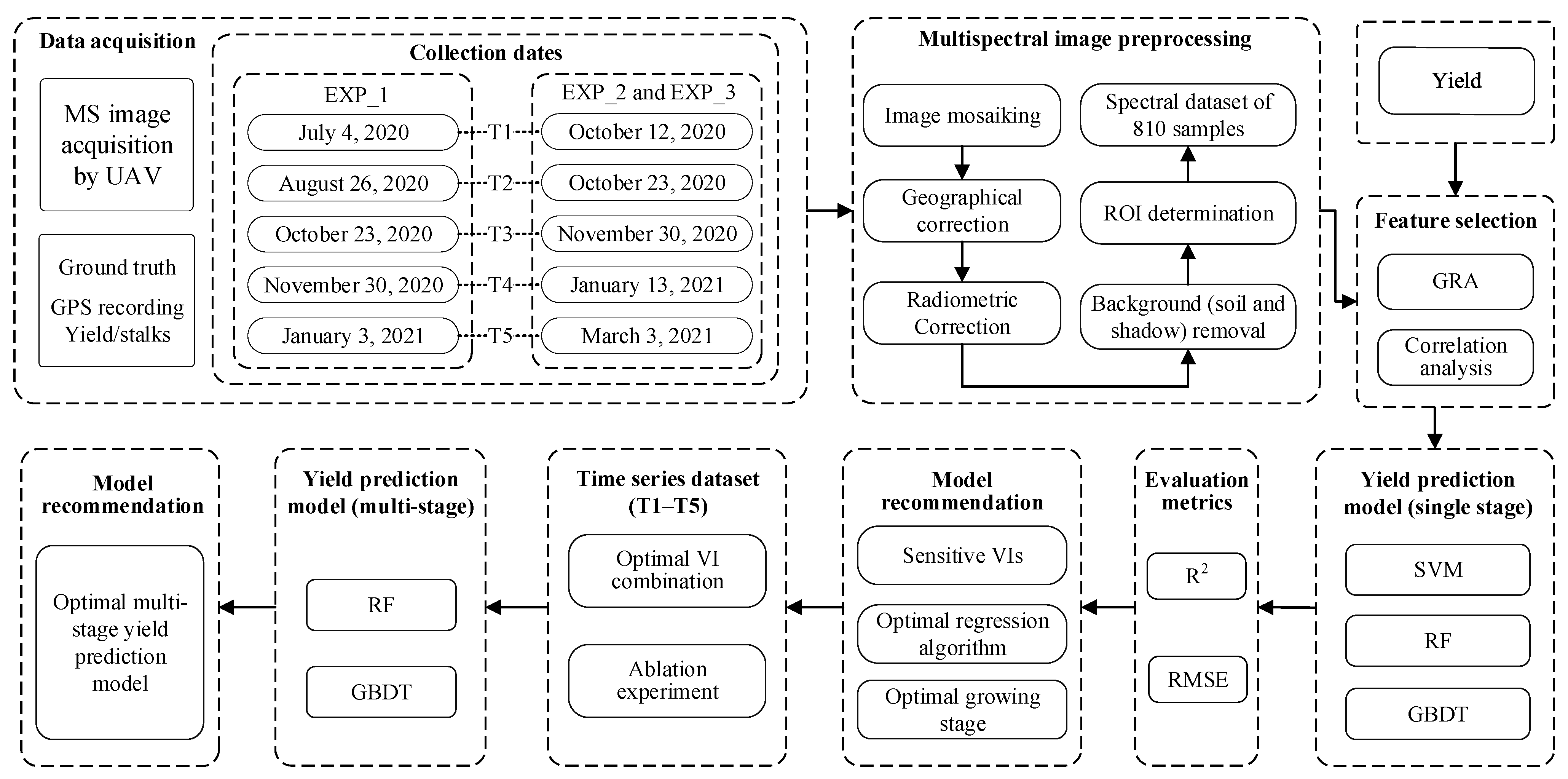
(1) To develop a hybrid feature selection method based on gray relational degree and correlation analysis (GRD-r) for extracting yield-sensitive VIs;

(2) To systematically evaluate the performance of prediction models constructed with different growth stage data and feature combinations using ensemble learning algorithms (GBDT, RF) and SVM;

(3) To determine optimal feature sets and establish robust regression models for both single-stage and multi-stage yield prediction scenarios.

2. Materials and Methods

2.1. Overall Research Route

The overall research framework is illustrated in Figure 1. Multispectral UAV imagery was acquired five times over the growing season from three experimental fields, covering both spring-planted and summer-planted sugarcanes. A variable selection strategy combining gray relational analysis and correlation analysis (GRD-r) was proposed. Supervised regression algorithms—including GBDT, RF, and SVM—were employed to develop both single-stage and multi-stage sugarcane yield prediction models. Finally, the effects of input features, crop growth stages, and modeling approaches on regression performance were analyzed to identify the optimal model for sugarcane yield prediction.

2.2. Data Acquisition

2.2.1. Study Area

From 2020 to early 2021, three experimental fields were established at the Subtropical Agricultural Science and Technology Innovation City of Guangxi University, denoted as EXP_1, EXP_2, and EXP_3, respectively (as shown in Figure 2). To enhance dataset diversity and improve model robustness, three different main sugarcane cultivars were planted across the three fields: Zhongzhe-6 (ZZ-6, cultivated by Guangxi University), Zhongzhe-9 (ZZ-9, cultivated by Guangxi University), and Guitang-42 (GT-42, cultivated by the Guangxi Academy of Agricultural Sciences). Each field varied in plot size and fertilizer treatment types, as listed in

Table 1. Experiment plan.

Experiment Field	Planting Date	Cultivar	Number of Plots	Plot Size	Fertilizer Type			Fertilization Amount (kg/hm2)
								FA0	FA0.5	FA1	FA1.5	FA2
EXP_1	28 April 2020	ZZ 6	15	15 m (ten rows) × 15 m (row length)	Insecticide mixed fertilizer with N–P–K of 17:7:12			0	940	1880	2820	3760
EXP_2	9 July 2020	ZZ 9	15	15 m (ten rows) × 13 m (row length)	Compound fertilizer with N–P–K of 18.6:9:15.3
EXP_3	9 July 2020	GT 42	9	10 m (seven rows) × 13 m (row length)	FT1	FT2	FT3	3000
					Non-biological organic fertilizer	Bio-organic fertilizer	Mixture (1:1)

Note: FT3 represents the fertilizer mixture of FT1 and FT2 in a 1:1 ratio.

. Both EXP_1 and EXP_2 had 15 plots, five fertilizer treatments, and three replicates, but with different fertilizer types: EXP_1 used insecticide-mixed fertilizers, while EXP_2 applied compound fertilizers. Each plot in EXP_1 and EXP_2 had ten rows of sugarcane, with a row space of 1.8 m, and row lengths of 15 m and 13 m, respectively. EXP_3 had 9 plots, three fertilizer treatments, and three replicates, Each treatment had the same amount of fertilizer, but different types—non-biological organic fertilizer, bio-organic fertilizer, and a 1:1 mixture of both. Each plot in EXP_3 had seven rows of sugarcane with a row space of 1.4 m and a row length of 13 m.

To expand the diversity of sugarcane, two different planting seasons were included. EXP_1 were spring-planted sugarcanes which were planted on 28 April 2020. The fertilizer was applied on two different dates; 20% were applied during planting, the remaining 80% were applied during the hilling-up process, which was conducted on 9 July 2020. Manual harvesting was carried out on 24 January 2021. EXP_2 and EXP_3 were summer-planted sugarcanes which were planted on 8 July 2020, with 20% basal fertilizer applied, followed by hilling-up fertilizer applied on 23 September 2020. Manual harvesting for those two fields was carried out on 8 March 2021.

2.2.2. Multispectral Remote Sensing Image Acquisition

Multispectral imagery was acquired by a five-band multispectral camera RedEdge (AgEagle Aerial Systems, Wichita, KS, USA), which was integrated on a four-rotor drone modeled M210 (DJI, Shenzhen, China), during five key growth stages of sugarcane: mid-tillering (T1), late-tillering (T2), mid-elongation (T3), late-elongation (T4), and maturity (T5), as shown in

Table 2. Brief information on multispectral imagery acquisition.

Serial Number	Growing Stage	Collection Dates		Image Quantity
		EXP_1	EXP_2/EXP_3	EXP_1	EXP_2/EXP_3
T1	Mid-tillering	July 4, 2020	October 12, 2020	483	279
T2	Late-tillering	August 26, 2020	October 23, 2020	483	279
T3	Mid-elongation	October 23, 2020	November 30, 2020	483	279
T4	Late-elongation	November 30, 2020	January 13, 2021	483	279
T5	Ripening	January 3, 2021	March 3, 2021	483	279

. The center wavelengths of RedEdge are 475 nm (Blue, B), 560 nm (Green, G), 668 nm (Red, R), 717 nm (Red Edge), and 840 nm (Near-Infrared, NIR). All flights were conducted under clear, windless, and cloud-free weather condition to maximumly avoid the spectral error caused by unstable weather. Four tarps of different levels of reflectance were placed at the open space by each field. Flights were performed at an altitude of 40–50 m, with the camera lens oriented vertically downward. Both the forward and side overlap were set at 85% to ensure high-quality mosaicking. The MS image had a ground sample distance of 2.86–3.58 cm.

The multispectral images acquired by UAV were first mosaicked using Pix4D Mapper (Pix4D, Prilly, Switzerland) and subsequently processed in ENVI 5.5 (NV5 Geospatial Software, Broomfield, CO, USA) and ArcGIS 10.7 (Esri, Redlands, CA, USA) for radiometric correction, geometric correction, image cropping, background removal, and dataset construction. The radiometric correction converted the DN values to reflectance which was performed with the four tarps by the empirical line method in ENVI. The main task of geometric correction is aligning the coordinate system of the MS images to that of the ground investigation. It was carried out by the ground control points preset before the flights. Image cropping was conducted in ArcGIS along the boundary of each field. Background removal was conducted by SVM classification to mainly remove the soil to ensure the accurate extraction of VIs. Taking the T2-stage imagery as an example, the processing results of some procedures with the yield investigation grids are shown in Figure 3. The spectral feature of each grid was determined by averaging all the pixels inside it. A time-series dataset was finally constructed by processing all the MS images of all the five stages. The dataset was further split into training and validation sets using stratified sampling based on the fertilizer treatments, with a ratio of 4:1.

2.2.3. Yield Data Acquisition

In each experimental field, three or five central rows (10 m in length) were selected within each plot for yield investigation. During yield investigation, each selected row was precisely recorded by RTK GPS. Each central row was then segmented into five grids of approximately 1.4 m × 2 m in size, as shown in Figure 4. The total yield for each plot and the number of stalks for each selected row were recorded. Across the three experimental fields, a total of 162 rows in 39 plots were surveyed, resulting in 39 plot-level yield values (t/hm²) and 162 effective stalk count measurements (stalks/hm²). The plot-level yields were first divided into 162 row-level yields according to the stalk count of each row, and then further expanded into 810 grid-level yields according to the vegetation coverage ratio of the grids, resulting in a total of 810 yield samples. The scatter plot of the yield data is presented in Figure 5. Significant yield variability was observed among different experimental fields, with EXP_1 showing the highest yield and EXP_3 the lowest.

2.3. Analysis Methods

2.3.1. Vegetation Indices

VIs are calculated using the reflectance values of two or more spectral bands and are designed to reduce background and illumination effects while enhancing the spectral signature of vegetation. They enable reliable temporal and spatial comparisons of crop canopy characteristics. In this study, 16 commonly used VIs (listed in

Table 3. VIs chosen in this study.

Vegetation Index	Computing Formula	Reference
Normalized Difference Vegetation Index (NDVI)	$\mathit{N}\mathit{D}\mathit{V}\mathit{I}={\displaystyle \frac{\left(\mathit{N}\mathit{I}\mathit{R}-\mathit{R}\right)}{\left(\mathit{N}\mathit{I}\mathit{R}+\mathit{R}\right)}}$	[28]
Soil-Adjusted Vegetation Index (SAVI)	$SAVI=1.5{\displaystyle \frac{\left(NIR-R\right)}{\left(NIR+R+0.5\right)}}$	[29]
Renormalized Difference Vegetation Index (RDVI)	$RDVI={\displaystyle \frac{\left(NIR-R\right)}{\sqrt{NIR+R}}}$	[30]
Wide Dynamic Range Vegetation Index (WDRVI)	$WDRVI={\displaystyle \frac{\left(0.2NIR-R\right)}{\left(0.2NIR+R\right)}}$	[31]
Transformed Difference Vegetation Index (TDVI)	$\mathit{T}\mathit{D}\mathit{V}\mathit{I}={\displaystyle \frac{1.5\left(\mathit{N}\mathit{I}\mathit{R}-\mathit{R}\right)}{\sqrt{\mathit{N}\mathit{I}{\mathit{R}}^2+\mathit{R}+0.5}}}$	[32]
Enhanced Vegetation Index (EVI)	$EVI=2.5{\displaystyle \frac{\left(NIR-R\right)}{\left(NIR+6R-7.5B+1\right)}}$	[33]
Ratio Vegetation Index 2 (RVI2)	$RV{I}_2={\displaystyle \frac{NIR}{G}}$	[34]
Simple Ratio Index (SR)	$SR={\displaystyle \frac{NIR}{R}}$	[35]
Modified Simple Ratio Index (MSRI)	$\mathit{M}\mathit{S}\mathit{R}\mathit{I}={\displaystyle \frac{\left(\frac{\mathit{N}\mathit{I}\mathit{R}}{\mathit{R}}-1\right)}{\left(\sqrt{\frac{\mathit{N}\mathit{I}\mathit{R}}{\mathit{R}}}+1\right)}}$	[36]
Non-Linear Index (NLI)	$\mathit{N}\mathit{L}\mathit{I}={\displaystyle \frac{\left(\mathit{N}\mathit{I}{\mathit{R}}^2-\mathit{R}\right)}{\left(\mathit{N}\mathit{I}{\mathit{R}}^2+\mathit{R}\right)}}$	[37]
Modified Non-Linear Index (MNLI)	$MNLI={\displaystyle \frac{1.5\left(NI{R}^2-R\right)}{\left(NI{R}^2+R+0.5\right)}}$	[38]
Difference Vegetation Index (DVI)	$\mathit{D}\mathit{V}\mathit{I}=\mathit{N}\mathit{I}\mathit{R}-\mathit{R}$	[39]
Green Difference Vegetation Index (GDVI)	$GDVI=NIR-G$	[40]
Simple Ratio Pigment Index (SRPI)	$\mathit{S}\mathit{R}\mathit{P}\mathit{I}={\displaystyle \frac{\mathit{B}}{\mathit{R}}}$	[41]
Normalized Pigment Chlorophyll Index (NPCI)	$NPCI={\displaystyle \frac{\left(R-B\right)}{\left(R+B\right)}}$	[41]
Normalized Green–Blue Difference Index (NGBDI)	$NGBDI={\displaystyle \frac{\left(G-B\right)}{\left(G+B\right)}}$	[42]

Note: B, G, R, and NIR represent the spectral reflectance at 475 ± 10 nm (blue), 560 ± 10 nm (green), 668 ± 5 nm (red), and 840 ± 20 nm (NIR), respectively.

) were selected for further analysis.

2.3.2. Correlation Analysis

Correlation analysis [43] is used to evaluate the degree of the linear relationship between two variables by calculating the correlation coefficient (r), which can be computed using Equation (1).

$$\mathit{r}={\displaystyle \frac{{\sum }_{\mathit{i}=1}^{\mathit{n}}\left({\mathit{x}}_{\mathit{i}}-\overline{\mathit{x}}\right)\left({\mathit{y}}_{\mathit{i}}-\overline{\mathit{y}}\right)}{\sqrt{{\sum }_{\mathit{i}=1}^{\mathit{n}}{\left({\mathit{x}}_{\mathit{i}}-\overline{\mathit{x}}\right)}^2}\sqrt{{\sum }_{\mathit{i}=1}^{\mathit{n}}{\left({\mathit{y}}_{\mathit{i}}-\overline{\mathit{y}}\right)}^2}}}$$

(1)

where n represents the sample size, x_i and y_i denote the values of sample i, and $\overline{x}$ and $\overline{y}$ represent the mean values of the n samples.

The higher the absolute value of r, the stronger the linear correlation between the two variables. Generally, 0.7 ≤ |r| < 1 indicates a very strong correlation, 0.4 ≤ |r| < 0.7 indicates a significant correlation, and |r| < 0.4 suggests a weak correlation. Correlation analysis serves multiple purposes in modeling, including the following: (1) evaluating the correlation between input variables and the target variable to identify sensitive features; and (2) assessing inter-variable correlations to avoid selecting highly correlated variables simultaneously, thereby reducing redundancy and improving the overall representational efficiency of the model.

2.3.3. Gray Relational Analysis

Gray relational analysis (GRA), also known as the gray relational degree analysis [44], is a key component of gray system theory. Its core principle is to determine the relative importance of variables in representing the dependent variable by calculating the gray relational degree (GRD). A higher GRD indicates a stronger consistency between the variation trends of the variable and the dependent variable. Therefore, GRA can be effectively used to identify the most influential variables [45].

Let the reference sequence be denoted as $X_0=\left\{x_0\left(k\right),k=\mathrm{1,2},\dots ,n\right\}$, and the comparison sequence as $X_i=\left\{x_i\left(k\right),k=\mathrm{1,2},\dots ,n\right\}$. The GRD between X₀ and X_i can be calculated using Equations (2) and (3).

$$\mathit{G}\mathit{R}\mathit{D}={\displaystyle \frac{1}{\mathit{n}}}{\sum }_{\mathit{k}=1}^{\mathit{n}}\mathit{\gamma }\left({\mathit{x}}_0\left(\mathit{k}\right),{\mathit{x}}_{\mathit{i}}\left(\mathit{k}\right)\right)$$

(2)

$$\mathit{\gamma }\left({\mathit{x}}_0\left(\mathit{k}\right),{\mathit{x}}_{\mathit{i}}\left(\mathit{k}\right)\right)={\displaystyle \frac{\underset{\mathit{i}}{\mathit{m}\mathit{i}\mathit{n}}\underset{\mathit{k}}{\mathit{m}\mathit{i}\mathit{n}}\left|{\mathit{x}}_0\left(\mathit{k}\right)-{\mathit{x}}_{\mathit{i}}\left(\mathit{k}\right)\right|+\mathit{\rho }\underset{\mathit{i}}{\mathit{m}\mathit{a}\mathit{x}}\underset{\mathit{k}}{\mathit{m}\mathit{a}\mathit{x}}\left|{\mathit{x}}_0\left(\mathit{k}\right)-{\mathit{x}}_{\mathit{i}}\left(\mathit{k}\right)\right|}{\left|{\mathit{x}}_0\left(\mathit{k}\right)-{\mathit{x}}_{\mathit{i}}\left(\mathit{k}\right)\right|+\mathit{\rho }\underset{\mathit{i}}{\mathit{m}\mathit{a}\mathit{x}}\underset{\mathit{k}}{\mathit{m}\mathit{a}\mathit{x}}\left|{\mathit{x}}_0\left(\mathit{k}\right)-{\mathit{x}}_{\mathit{i}}\left(\mathit{k}\right)\right|}}$$

(3)

where ρ is the gray relational coefficient with a range of 0 to 1, which is set to 0.5 in this study.

In this study, the GRD between each spectral feature and sugarcane yield was calculated. Prior to the computation, all variables were normalized. Normally, a greater GRD value indicates that the corresponding spectral feature has a stronger influence on yield.

2.3.4. Regression Algorithms

To develop sugarcane yield prediction models, three supervised learning methods were employed: GBDT, RF, and SVM. SVM is a statistical learning model, while both RF and GBDT are ensemble learning algorithms. These three supervised learning algorithms can be applied to both classification and regression tasks. A brief introduction to each method is provided below.

• SVM

Support Vector Machine (SVM) is primarily a classification algorithm, and when applied to regression tasks, it is also referred to as Support Vector Regression (SVR) [46]. Similarly to its classification counterpart, SVM adopts the principle of maximum margin. It employs a kernel function to map the original input space into a high-dimensional feature space and utilizes an ε-insensitive loss function to construct a flexible “ε-tube” with a minimal radius around the target function. The algorithm seeks to fit the predicted values as closely as possible within this tube, thereby achieving linear regression and identifying the optimal decision function. SVM effectively avoids the “curse of dimensionality,” offering a strong generalization ability and high prediction accuracy.

2.

RF

Random Forest (RF) is a Bagging-based ensemble learning method in which individual decision trees are built independently of each other [47]. The algorithm is nearly identical for both classification and regression tasks, with the primary difference being that regression uses Mean Squared Error (MSE) as the criterion for tree growth. Specifically, during tree construction, the algorithm selects the child node that results in the minimum MSE relative to the parent node, and continues this process recursively until a complete tree is formed. The final prediction is obtained by computing the weighted average of all leaf node outputs across the ensemble.

3.

GBDT

Gradient Boosting Decision Tree (GBDT) is a Boosting-based ensemble learning method in which individual decision trees are built sequentially and are dependent on each other [48]. Unlike RF, which builds trees independently, GBDT constructs trees in a stage-wise manner. In each iteration, a new weak learner is trained to fit the residual errors of the previous model, thereby updating the model parameters in the direction that minimizes the loss function.

4.

Parameter settings

Grid search (GS) was employed for the hyperparameter tuning of the regression models, aiming to identify the optimal combination of hyperparameters that minimizes the validation error. The selected parameters for each model are summarized in

Table 4. The hyperparameters of the regression models.

Model	Hyperarameter	Description	Searching Grid	Optimal Hyperparameter
SVM	kernel	Kernel function	[linear, poly, rbf, sigmoid]	poly
	C	Penalty	[0.001, 0.01, 0.1, 1, 5, 10, 20, 50]	20
	gamma	Kernel coefficient	[0.001, 0.01, 0.1, 1, 5, 10, 20, 50]	10
RF	max_depth	Maximum depth of each tree	[5, 10, 15, 20, 50, 100]	50
	n_estimators	Number of trees	[50, 100, 200, 300, 500]	100
	max_leaf_nodes	Maximum number of leaf nodes	[2, 5, 10, 20, 30, 50, 100]	50
	min_samples_leaf	Minimum number of samples required at a leaf node	[2, 5, 10, 20]	5
	min_samples_split	Minimum number of samples required to split a node	[2, 5, 10, 20, 50]	10
GBDT	max_depth	Maximum depth of each tree	[1, 3, 5, 7, 10, 15, 20, 50, 100]	3
	n_estimators	Number of trees	[100, 200, 300, 400, 500, 600, 700, 1000]	200
	learning_rate	Learning rate	[0.01, 0.02, 0.03, 0.04, 0.05, 0.06, 0.1]	0.05
	loss	Loss function	[‘squared_error’, ‘absolute_error’, ‘huber’]	‘squared_error‘

.

2.3.5. Model Performance Evaluation

To evaluate the accuracy of both the yield loss prediction model and the yield prediction model, two metrics were primarily used: the Coefficient of Determination (R²) and the Root Mean Square Error (RMSE). R² (Equation (4)) reflects the goodness of fit between the predicted and actual values, while RMSE (Equation (5)) directly measures the prediction error of the model.

$${\mathit{R}}^2=1-{\displaystyle \frac{{\sum }_{\mathit{i}=1}^{\mathit{n}}{\left({\mathit{y}}_{\mathit{i}}-{\widehat{\mathit{y}}}_{\mathit{i}}\right)}^2}{{\sum }_{\mathit{i}=1}^{\mathit{n}}{\left({\mathit{y}}_{\mathit{i}}-\overline{\mathit{y}}\right)}^2}}$$

(4)

$$\mathit{R}\mathit{M}\mathit{S}\mathit{E}=\sqrt{{\displaystyle \frac{1}{\mathit{n}}}{\sum }_{\mathit{i}=1}^{\mathit{n}}{\left({\mathit{y}}_{\mathit{i}}-{\widehat{\mathit{y}}}_{\mathit{i}}\right)}^2}$$

(5)

where $y_i$ and ${\widehat{y}}_i$ represent the actual value and the estimated value of sample I, respectively; and $\overline{y}$ represents the mean value of the n samples.

3. Results

3.1. Sensitive Spectral Feature Selection

The large number of spectral bands/VI, and their potentially high inter-variable correlation, could directly complicate the yield prediction model and even cause performance deterioration. GRA and correlation analysis were performed to evaluate the relationship between spectral features at different growth stages and the yield, and thus help in selecting the sensitive spectral features. The results in

Table 5. GRA and correlation analysis results between each spectral feature and the yield.

Spectral Feature	Growing Stages
	T1		T2		T3		T4		T5
	GRD	r	GRD	r	GRD	r	GRD	r	GRD	r
B	0.73	0.51	0.76	0.07	0.61	−0.66	0.77	0.24	0.70	−0.24
G	0.76	0.52	0.70	−0.28	0.64	−0.61	0.70	−0.44	0.73	0.04
R	0.76	0.42	0.66	−0.65	0.66	−0.69	0.64	−0.69	0.64	−0.53
RE	0.76	0.52	0.71	−0.24	0.61	−0.43	0.67	−0.59	0.72	0.34
NIR	0.78	0.72	0.77	0.62	0.55	0.65	0.78	0.55	0.71	0.67
WDRVI	0.62	−0.28	0.83	0.78	0.75	0.76	0.77	0.71	0.79	0.71
TDVI	0.69	0.28	0.77	0.76	0.58	0.79	0.78	0.70	0.72	0.74
SRPI	0.78	0.75	0.79	0.74	0.57	0.35	0.71	0.67	0.79	0.62
MSRI	0.64	−0.27	0.84	0.77	0.69	0.76	0.77	0.71	0.80	0.70
SR	0.65	−0.26	0.83	0.77	0.74	0.76	0.77	0.71	0.81	0.69
SAVI	0.67	0.08	0.78	0.78	0.57	0.78	0.78	0.70	0.72	0.74
RVI2	0.61	−0.41	0.83	0.72	0.64	0.74	0.78	0.68	0.77	0.69
RDVI	0.66	0.01	0.78	0.78	0.57	0.78	0.78	0.71	0.72	0.74
NPCI	0.61	−0.74	0.60	−0.74	0.72	−0.34	0.51	−0.67	0.60	−0.62
NGBDI	0.56	−0.53	0.58	−0.46	0.62	0.67	0.52	−0.54	0.74	0.68
NDVI	0.62	−0.29	0.81	0.78	0.54	0.76	0.75	0.71	0.75	0.72
MNLI	0.66	0.03	0.79	0.76	0.80	0.80	0.79	0.70	0.78	0.73
NLI	0.67	−0.02	0.76	0.80	0.76	0.79	0.77	0.70	0.72	0.73
EVI	0.72	0.37	0.79	0.78	0.58	0.79	0.77	0.69	0.75	0.73
GDVI	0.76	0.48	0.79	0.71	0.59	0.77	0.78	0.64	0.70	0.73
DVI	0.75	0.48	0.78	0.73	0.59	0.79	0.79	0.69	0.72	0.73
Minimum	0.56	0.01	0.58	0.07	0.54	0.34	0.51	0.24	0.60	0.04
Maximum	0.78	0.75	0.84	0.80	0.80	0.80	0.79	0.71	0.81	0.74
Average	0.689	0.380	0.760	0.653	0.637	0.689	0.732	0.640	0.732	0.625
Standard Deviation	0.065	0.424	0.070	0.534	0.077	0.557	0.081	0.541	0.049	0.426

Note: Bold represents GRD rankings in the top three, and gray shading represents that both GRD and |r| are greater than 0.7.

showed that all spectral features had a GRD greater than 0.5 with yield, indicating a moderate to strong association. The average GRD values for the five growth stages (T1 to T5) were 0.689, 0.760, 0.637, 0.732, and 0.732, respectively, with the lowest observed in T3. The highest GRD values at each stage were approximately 0.8, corresponding to the NIR band and SRPI (0.78) at T1, MSRI (0.84) at T2, MNLI (0.80) at T3, MNLI and DVI (both 0.79) at T4, and SR (0.81) at T5. The average correlation coefficients between spectral features and yield at each stage were 0.380, 0.653, 0.689, 0.640, and 0.625, respectively, with the highest observed at T3. These results suggest that the spectral features of the sugarcane canopy throughout the entire growth stage demonstrate good representational ability for yield prediction.

The correlation analysis among VIs is presented in Figure 6. To reduce variable redundancy, VIs with low mutual correlations are considered more informative for modeling. At the T1 stage, most VIs exhibited strong correlations (greater than 0.7). However, GDVI and DVI showed low correlations (below 0.5) with WDRVI, SRPI, SR, RVI2, NPCI, NGBDI, and MSRI. In addition, SPRI and NPCI exhibited low correlations with the majority of other VIs. At the T2 stage, only NGBDI showed slightly lower correlations with other indices, with correlation coefficients around 0.6. At the T3 stage, SPRI and NPCI again displayed relatively weak correlations with the rest, all below 0.5. During the T4 stage, only NGBDI and GDVI had slightly lower correlations with other indices, but their values remained relatively high—around 0.9. At the T5 stage, NGBDI was the only index with noticeably lower correlations, around 0.7.

When selecting sensitive VIs, both the GRD and the absolute correlation coefficient (|r|) with yield should be jointly considered. Accordingly, the following three criteria were established for selecting yield-sensitive VIs:

(1)

The initially selected VIs should have a relatively high GRD with yield (for example, ranked in the top 30%);

(2)

The initially selected VIs should have a relatively high correlation with yield (for example, ranked in the top 30%);

(3)

The selected VIs should exhibit relatively low correlation with each other (for example, |r| < 0.6). If a significant correlation is observed, change to other VIs with a lower GRD or correlation.

Based on these principles, the selection process involved the following: first, identifying VIs with top-ranked GRD or |r| values with respect to yield; second, in cases where these VIs were highly correlated with each other (in this case, |r| close to 1), retaining only one of them; and finally, when VIs had similar GRD or |r| values, giving preference to the ones with a lower correlation with other VIs. This feature selection strategy is referred to in this study as GRD-r.

Based on the results of Table 5 and Figure 6, the recommended sensitive VIs for each growth stage are summarized in

Table 6. Recommended sensitive VIs for each growing stage based on GRD-r criterion.

Growing Stage	Sensitive VIs
	Highly Recommended	Next Recommended
T1	SRPI, NPCI, GDVI, NGBDI	DVI, EVI
T2	WDRVI, MSRI (SR), NLI (MNLI), RVI2	RDVI, NGBDI
T3	WDRVI, MSRI (SR), NLI (MNLI),TDVI	NGBDI, SPRI, NPCI
T4	WDRVI, MSRI (SR), NLI (MNLI), NDVI	NGBDI, GDVI
T5	SAVI, TDVI, RDVI, MSRI (SR)	NGBDI

.

3.2. Single-Stage Sugarcane Yield Prediction Model

3.2.1. Yield Prediction Model Based on Sensitive VIs Extracted by Different Criteria

Yield prediction models were developed using variable combinations consisting of 1–3 VIs selected by three different feature selection criteria for each stage. The top-performing models of T3 are summarized in

Table 7. Yield prediction results based on VIs selected by different criteria in T3 stage.

Feature Extraction Criterion	Model Input Variables			Modeling Method	Training Set		Validation Set
	V1	V2	V3		${\mathit{R}}_{\mathit{c}}^2$	RMSEC (RMSEc t/hm2)	${\mathit{R}}_{\mathit{v}}^2$	RMSEVRMSEv (t/hm2)
GRD/r	MNLI			GBDT	0.74	7.80	0.67	9.13
				RF	0.72	8.05	0.69	8.83
	NLI			GBDT	0.75	7.58	0.67	9.10
				RF	0.73	7.87	0.65	9.45
	WDRVI			GBDT	0.74	7.78	0.67	9.19
				RF	0.73	7.92	0.64	9.52
GRD	WDRVI	NLI	SR	GBDT	0.80	6.78	0.69	8.78
				RF	0.79	6.89	0.68	9.00
r	TDVI	NLI	EVI	GBDT	0.80	6.84	0.70	8.76
				RF	0.80	6.77	0.71	8.57
GRD-r	WDRVI	NGBDI		GBDT	0.83	6.33	0.76	7.76
				RF	0.82	6.48	0.75	7.94
	SR	NGBDI		GBDT	0.83	6.25	0.76	7.82
				RF	0.82	6.40	0.74	8.11
	MNLI	NGBDI		GBDT	0.80	6.86	0.73	8.27
				RF	0.79	6.98	0.73	8.26
	WDRVI	NGBDI	TDVI	GBDT	0.83	6.19	0.77	7.63
				RF	0.83	6.31	0.76	7.73
	WDRVI	NGBDI	GDVI	GBDT	0.83	6.21	0.76	7.71
				RF	0.83	6.30	0.77	7.62
	MNLI	NGBDI	WDRVI	GBDT	0.84	6.11	0.76	7.78
				RF	0.83	6.32	0.77	7.65

Note: Bold represents the optimal modeling results for different input variables, and GRD/r represents that the GRD and |r| between the input variable and the yield are in the top three, which is the same below.

. The representative results of the other four stages are given in Table S1–S4 as the Supplementary Materials. Specifically, the “GRD/r” criterion indicates the selection of the VI that exhibits the highest value based on either GRD or |r|; the “GRD” or “r” criterion refers to the selection of the top three VIs ranked by their GRD or |r|, respectively; and the “GRD-r” criterion refers to the combined feature selection strategy introduced in Section 3.1. The results indicate the following: (1) Models based on “GRD-r”-selected VIs had the highest accuracy, and even the models only based on two “GRD-r”-selected VIs could outperform the models based on three “GRD”-selected or “r”-selected VIs. (2) GBDT and RF showed similar performance in yield prediction.

A detailed analysis of the input variables used in the three optimal prediction models reveals the following:

(1) MNLI ranked first in both GRD (0.76) and |r| (0.79) with yield, which explains why the single-variable model based on MNLI achieved the best performance.

(2) In the case of the two-variable model, only NPCI and SRPI had low correlations with MNLI (|r| < 0.6); however, their correlations with yield (|r| < 0.4) did not meet the basic criterion for feature selection. In contrast, NGBDI and WDRVI both showed relatively high correlations with MNLI (|r| = 0.89 and 0.87, respectively), and also exhibited strong associations with yield, with both GRD and |r| exceeding 0.6. Consequently, the model combining WDRVI and NGBDI produced better predictive performance.

(3) For the three-variable models, the GBDT model based on WDRVI, NGBDI, and TDVI and the RF model based on WDRVI, NGBDI, and GDVI both achieved the highest performance ($R_v^2$ = 0.77). This is because TDVI and GDVI had relatively low correlations with WDRVI and NGBDI (<0.7), while TDVI showed the highest correlation with yield (|r| = 0.79) and GDVI had the highest GRD with yield (GRD = 0.59). These results align well with the “GRD-r” feature selection criterion proposed in this study.

3.2.2. The Effectiveness Experiment of the “GRD-r” Criterion

To better demonstrate the advantages of the “GRD-r” criterion in terms of both accuracy and efficiency, we further compared the GBDT model performance based on sensitive VIs selected by different criteria—both before and after combining them with the original five-band spectral reflectance. The results are presented in

Table 8. Yield prediction results based on different VIs by GBDT for each growing stage.

Growing Stage	Model Code	Feature Extraction Criterion	Modeling VIs			Modeling Result Only Based on VIs		Modeling Result Based on the Conbination of VIs and The Five-Band Reflectance
			V1	V2	V3	${\mathit{R}}_{\mathit{v}}^2$	RMSEV (t/hm2)	${\mathit{R}}_{\mathit{v}}^2$	RMSEV (t/hm2)
T1	1	GRD-r	SRPI	DVI	NGBDI	0.70	8.69	0.68	8.94
	2	GRD	SRPI	GDVI	DVI	0.67	9.09	0.69	8.80
	3	r	SRPI	NPCI	NGBDI	0.67	9.17	0.66	9.20
T2	4	GRD-r	NLI	NGBDI	RVI2	0.73	8.28	0.74	8.12
	5	GRD	WDRVI	SR	RVI2	0.68	9.03	0.72	8.44
	6	r	RDVI	NLI	NDVI	0.69	8.87	0.75	7.99
T3	7	GRD-r	WDRVI	NGBDI	TDVI	0.77	7.63	0.76	7.81
	8	GRD	WDRVI	NLI	SR	0.69	8.78	0.74	8.05
	9	r	TDVI	NLI	EVI	0.70	8.76	0.74	8.05
T4	10	GRD-r	NDVI	GDVI	NGBDI	0.66	9.26	0.67	9.14
	11	GRD	MNLI	GDVI	DVI	0.65	9.46	0.64	9.57
	12	r	WDRVI	NDVI	MSRI	0.57	10.37	0.63	9.70
T5	13	GRD-r	MSRI	RVI2	SRPI	0.69	8.83	0.69	8.91
	14	GRD	MSRI	SRPI	WDRVI	0.64	9.47	0.67	9.13
	15	r	SAVI	RDVI	TDVI	0.60	10.08	0.67	9.07

Note: Bold represents the optimal modeling results in each growing stage.

and Figure 7. The $R_v^2$ of the 15 GBDT models increased by an average of 3.45% after involving the five-band reflectance, but for models developed based on the “GRD-r” criterion, the accuracy remained largely unchanged, with the average $R_v^2$ of the 15 GBDT models even slightly decreasing by 0.25%. In contrast, the $R_v^2$ of the 15 GBDT models simply based on GRD and r criterion increased by 3.85% and 7.02%, respectively. These results suggest that the variable sets selected using the “GRD-r” criterion possess sufficient and comprehensive information, whereas those selected using GRD or r alone may be relatively less informative.

3.3. Multi-Temporal Yield Prediction Model

3.3.1. Multi-Temporal Yield Prediction Model Based on Sensitive Features Selected Using Different Criteria

Each optimal single-stage model included three sensitive Vis, as shown in Table 8. However, if all these VIs were used to construct a multi-stage yield prediction model, the large number of variables might lead to the curse of dimensionality. Therefore, to reduce the dimensionality while retaining key spectral information, only one sensitive VI was randomly selected for each growth stage to form three sets of combinations, each set containing 3⁵ combinations, and both the GBDT and RF models were developed based on every combination. The best result for each feature selection criterion is summarized in

Table 9. The best results obtained under each feature extraction criterion.

Feature Extraction Criterion	Model Variables					Modeling Method	Training Set		Validation Set
	T1	T2	T3	T4	T5		${\mathit{R}}_{\mathit{c}}^2$	RMSEC (t/hm2)	${\mathit{R}}_{\mathit{v}}^2$	RMSEV (t/hm2)
GRD	DVI	RVI2	NLI	DVI	SRPI	GBDT	0.88	5.36	0.81	6.98
						RF	0.87	5.40	0.80	7.19
r	SRPI	NDVI	TDVI	MSRI	TDVI	GBDT	0.87	5.41	0.79	7.20
						RF	0.87	5.55	0.80	7.11
GRD-r	DVI	NDVI	TDVI	NDVI	SRPI	GBDT	0.89	5.28	0.83	6.63
						RF	0.87	5.47	0.82	6.80

Note: Bold represents the optimal modeling results among different types of feature extraction criterion.

. Consistent with the single-stage models, the multi-stage yield prediction model based on the “GRD-r” criterion achieved the highest accuracy. Specifically, the GBDT model built using DVI (T1), NDVI (T2), TDVI (T3), NDVI (T4), and SRPI (T5) achieved the best performance, with $R_v^2$ = 0.83 and RMSE_V = 6.63 t/hm². The scatter plot of the predicted yields versus the ground truth for this optimal model is shown in Figure 8. The red lines represent the trend of “y = x”. The predicted values in both the training and validation set closely follow the red lines, implying the low systematic error of our model.

3.3.2. Contribution Analysis of Sensitive VIs from Different Stages Based on the ‘GRD-r’ Criterion

To further evaluate the contribution of sensitive VIs from each growth stage to the yield prediction model, a sequential exclusion approach was applied. Specifically, one index from a single growth stage was removed at a time, and GBDT models were reconstructed using the remaining four VIs. The results are presented in

Table 10. Yield prediction results by GBDT based on four variables.

Model Code	Model Variables					Training set		Validation set
	T1	T2	T3	T4	T5	${\mathit{R}}_{\mathit{c}}^2$	RMSEC (t/hm2)	${\mathit{R}}_{\mathit{v}}^2$	RMSEV t/hm2)
Reference	DVI	NDVI	TDVI	NDVI	SRPI	0.89	5.28	0.83	6.63
Ⅰ		NDVI	TDVI	NDVI	SRPI	0.86	5.59	0.79	7.25
Ⅱ	DVI		TDVI	NDVI	SRPI	0.87	5.51	0.80	7.08
Ⅲ	DVI	NDVI		NDVI	SRPI	0.86	5.77	0.79	7.30
Ⅳ	DVI	NDVI	TDVI		SRPI	0.87	5.45	0.81	6.96
Ⅴ	DVI	NDVI	TDVI	NDVI		0.86	5.73	0.80	7.18

. Missing a VI from any growth stage will decrease the five-stage model. The performance degradation degree of each four-variable model is quite similar, with the largest reduction of 4.8% in $R_v^2$ for model Ⅲ, which lacks the VI of T3. These results indicate that canopy VIs from each growth stage contribute substantially to the overall accuracy of the yield prediction model.

4. Discussion

4.1. Performance Evaluation of Single-Stage Sugarcane Yield Prediction Models

As shown in Table 8, the yield prediction models constructed at the elongation stage (T3) achieved the highest accuracy. T3 had the highest average correlation coefficient but the lowest average GRD with yields. This indicates that the elongation stage plays a critical role in determining sugarcane yield, and correlation coefficient can be a more significant factor than GRD. The sensitive VIs selected using the “GRD-r” criterion yielded the best regression performance. While appropriately increasing the number of input variables can improve model accuracy, excessive variable inclusion may lead to overfitting or the curse of dimensionality. Therefore, in this study, the number of selected VIs was limited to no more than three. Notably, for VIs selected using the “GRD-r” criterion, adding spectral reflectance data slightly reduced model performance. In contrast, for indices selected using GRD or |r| alone, model accuracy improved after the addition of reflectance data. This indicates that selecting features based solely on GRD or |r| tends to introduce feature homogeneity and lacks comprehensiveness, which may compromise model performance. The proposed “GRD-r” feature selection criterion, by integrating both correlation and gray relational information, effectively identifies sensitive variables with broader information coverage. This facilitates a balanced trade-off between model complexity and predictive accuracy.

4.2. Performance Evaluation of Multi-Stage Sugarcane Yield Prediction Models

As shown in Table 9, the GBDT model built using DVI (T1), NDVI (T2), TDVI (T3), NDVI (T4), and SRPI (T5) was the optimal multi-stage yield prediction model which was built based on the “GRD-r” criterion. Its $R_v^2$ reaches 0.83, which is 7.8% higher than that of the best single-stage model—namely, the GBDT model at the T3 stage, with a $R_v^2$ of 0.77 as shown in Table 8. This highlights that the growth status at different sugarcane growth stages contributes significantly to the final yield. For example, the tillering stage is closely associated with effective stalk number, the elongation stage determines plant height, and the maturity stage affects sugar content—all of which are critical yield-determining factors. Therefore, yield prediction models constructed using the time-series variation in sensitive spectral features not only achieve higher performance but also offer stronger interpretability. The model built using spectral features from all five growth stages yields the highest accuracy. Removing any single stage results in decreased model performance, underscoring the importance of spectral information from each stage. Given that sugarcane has a relatively long growing cycle, this study acquired 1–2 sets of UAV-based multispectral data during each of the key stages: tillering, elongation, and maturity. This temporal coverage adequately reflected the growth dynamics of each stage. However, further reducing the data acquisition frequency would compromise the ability of time-series spectral features to capture physiological variations throughout the full growing season. Consequently, acquiring canopy spectral data across the entire growth cycle is essential to ensure that time-series features comprehensively represent stage-specific growth characteristics. This, in turn, enables the more accurate interpretation of yield variation trends and facilitates the construction of high-performance yield prediction models. In terms of feature selection, models based on the “GRD-r” criterion consistently outperformed those constructed using either GRD or |r| alone, further confirming the effectiveness of the GRD-r strategy in selecting informative and representative variables.

5. Conclusions

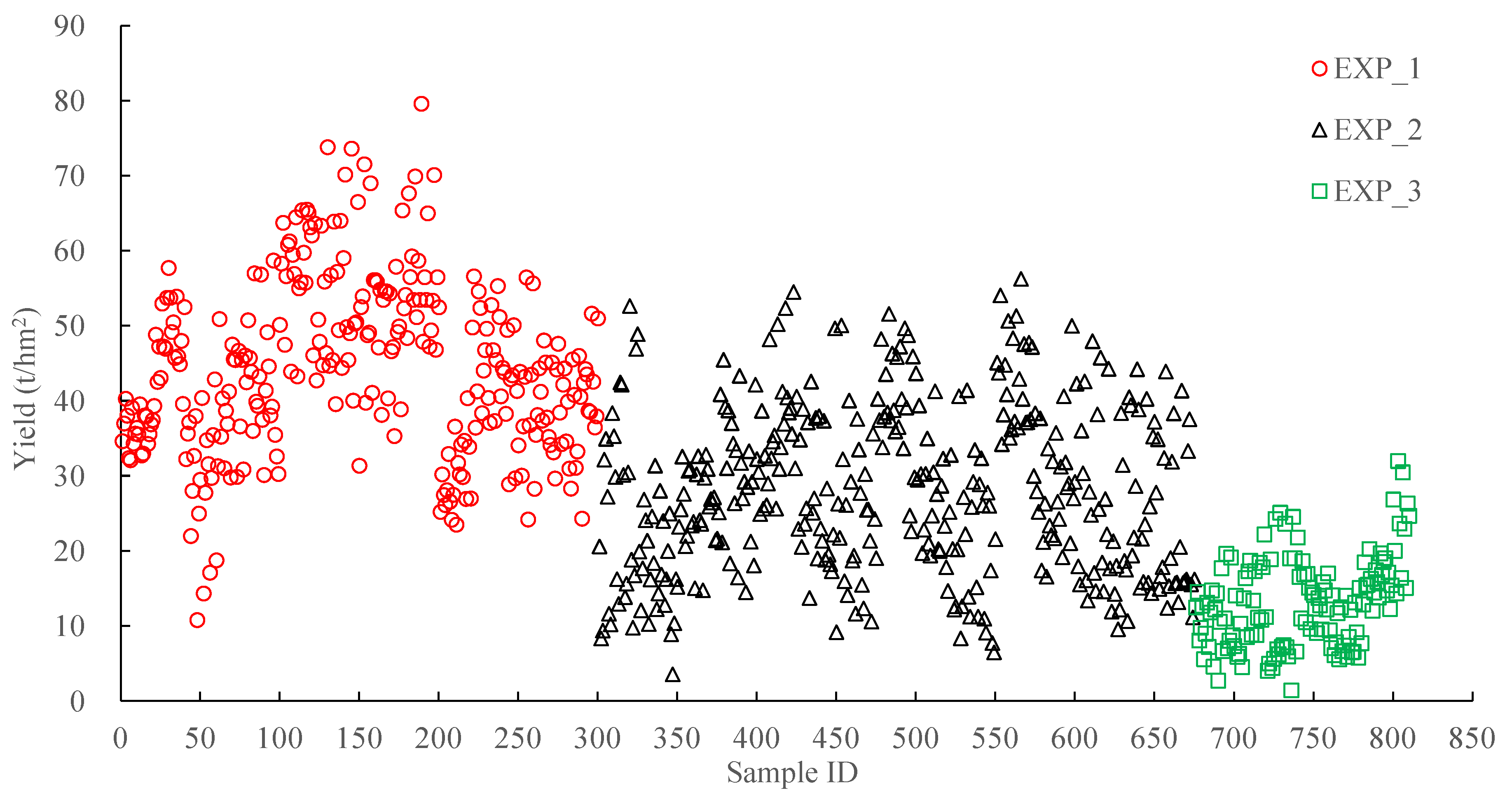
This study collected multi-temporal multispectral imagery from three sugarcane experimental fields under different fertilization treatments to analyze the relationship between spectral features and yield. A feature selection criterion of sensitive VIs for yield prediction was proposed. Sugarcane yield prediction models with the least variables were built both for a single-growth-stage scenario and a multi-growth-stage scenario. The main conclusions were as follows:

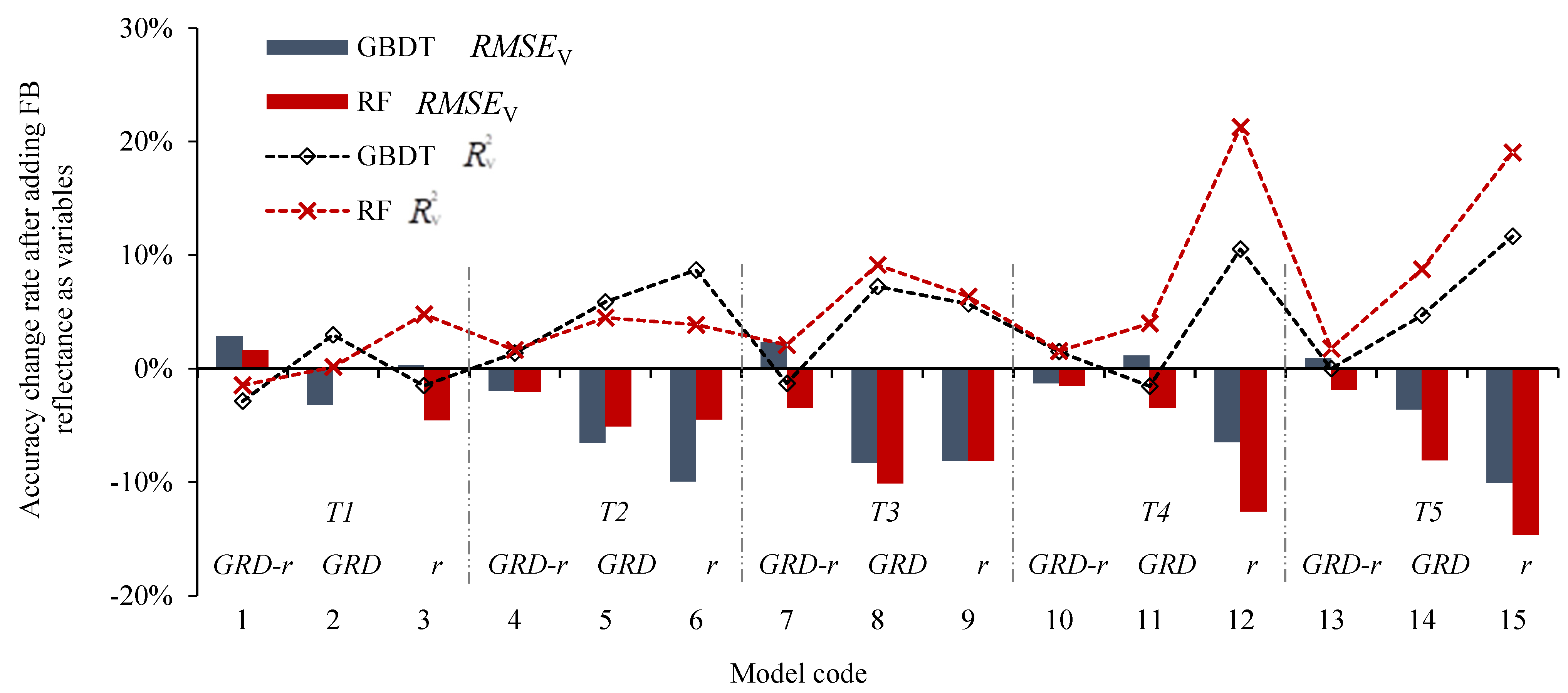
(1) A variable selection criterion named “GRD-r” was proposed, which integrated both GRA and correlation analysis among variables. The core idea was that when selecting yield prediction variables, both the GRD and |r| values with respect to yield should be considered. The selected VIs should exhibit a high GRD or |r| with yield, while maintaining relatively low inter-correlations (|r|) among themselves.

(2) Yield prediction models constructed using sensitive VIs selected based on the “GRD-r” criterion achieved the best performance.

(3) For the single-stage prediction, the GBDT model built at the T3 stage using WDRVI, NGBDI, and TDVI achieved the highest accuracy ($R_v^2$ = 0.77 and RMSE_V = 7.63 t/hm²).

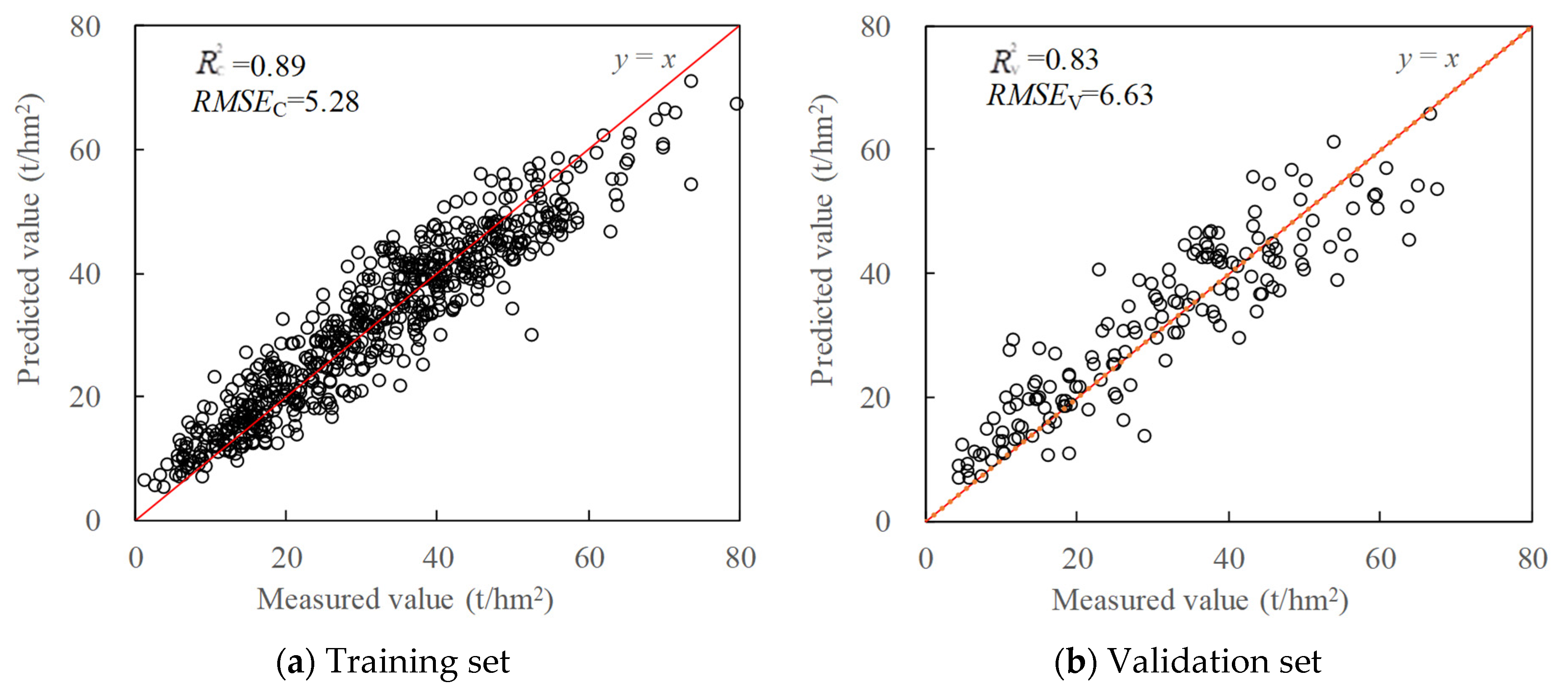
(4) For the multi-stage prediction, the GBDT model built from DVI (T1), NDVI (T2), TDVI (T3), NDVI (T4), and SRPI (T5) achieved the best overall performance ($R_v^2$= 0.83 and RMSE_V = 6.63 t/hm²).

References

1. Som-ard, J.; Atzberger, C.; Izquierdo-Verdiguier, E.; Vuolo, F.; Immitzer, M. Remote sensing applications in sugarcane cultivation: A review. Remote Sens. 2021, 13, 4040. [Google Scholar] [CrossRef]
2. Ban, H.Y.; Kim, K.S.; Park, N.W.; Lee, B.W. Using MODIS data to predict regional corn yields. Remote Sens. 2017, 9, 16. [Google Scholar] [CrossRef]
3. Zhou, L.; Tu, W.; Wang, C.; Li, Q. A heterogeneous access metamodel for efficient IoT remote sensing observation management: Taking precision agriculture as an example. IEEE Internet Things J. 2022, 9, 8616–8632. [Google Scholar] [CrossRef]
4. Barzin, R.; Pathak, R.; Lotfi, H.; Varco, J.; Bora, G.C. Use of UAS multispectral imagery at different physiological stages for yield prediction and input resource optimization in corn. Remote Sens. 2020, 12, 2392. [Google Scholar] [CrossRef]
5. Alexopoulos, A.; Koutras, K.; Ali, S.B.; Puccio, S.; Carella, A.; Ottaviano, R.; Kalogeras, A. Complementary use of ground-based proximal sensing and airborne/spaceborne remote sensing techniques in precision agriculture: A systematic review. Agronomy 2023, 13, 1942. [Google Scholar] [CrossRef]
6. Alvarez-Vanhard, E.; Corpetti, T.; Houet, T. UAV & satellite synergies for optical remote sensing applications: A literature review. Sci. Remote Sens. 2021, 3, 100019. [Google Scholar] [CrossRef]
7. Yang, G.; Liu, J.; Zhao, C.; Li, Z.; Huang, Y.; Yu, H.; Xu, B.; Yang, X.; Zhu, D.; Zhang, X.; et al. Unmanned aerial vehicle remote sensing for field-based crop phenotyping: Current status and perspectives. Front. Plant Sci. 2017, 8, 1111. [Google Scholar] [CrossRef]
8. Van Klompenburg, T.; Kassahun, A.; Catal, C. Crop yield prediction using machine learning: A systematic literature review. Comput. Electron. Agric. 2020, 177, 105709. [Google Scholar] [CrossRef]
9. Yuan, J.; Zhang, Y.; Zheng, Z.; Yao, W.; Wang, W.; Guo, L. Grain crop yield prediction using machine learning based on UAV remote sensing: A systematic literature review. Drones 2024, 8, 559. [Google Scholar] [CrossRef]
10. Adak, A.; Murray, S.C.; Božinović, S.; Lindsey, R.; Nakasagga, S.; Chatterjee, S.; Anderson, S.L., II; Wilde, S. Temporal vegetation indices and plant height from remotely sensed imagery can predict grain yield and flowering time breeding value in maize via machine learning regression. Remote Sens. 2021, 13, 2141. [Google Scholar] [CrossRef]
11. Peng, J.; Wang, D.; Zhu, W.; Yang, T.; Liu, Z.; Rezaei, E.E.; Li, J.; Sun, Z.; Xin, X. Combination of UAV and deep learning to estimate wheat yield at ripening stage: The potential of phenotypic features. Int. J. Appl. Earth Obs. Geoinf. 2023, 124, 103494. [Google Scholar] [CrossRef]
12. Tripathi, R.; Tripathy, B.R.; Jena, S.S.; Swain, C.K.; Mohanty, S.; Sahoo, R.N.; Nayak, A.K. Prediction of rice yield using sensors mounted on unmanned aerial vehicle. Agric. Res. 2024, 13, 1–11. [Google Scholar] [CrossRef]
13. Li, X.; Chen, M.; He, S.; Xu, X.; He, L.; Wang, L.; Gao, Y.; Tang, F.; Gong, T.; Wang, W.; et al. Estimation of soybean yield based on high-throughput phenotyping and machine learning. Front. Plant Sci. 2024, 15, 1395760. [Google Scholar] [CrossRef] [PubMed]
14. Shen, Y.; Mercatoris, B.; Cao, Z.; Kwan, P.; Guo, L.; Yao, H.; Cheng, Q. Improving wheat yield prediction accuracy using LSTM-RF framework based on UAV thermal infrared and multispectral imagery. Agriculture 2022, 12, 892. [Google Scholar] [CrossRef]
15. Yadav, A.; Shukla, A.K. Prediction of maize crop yield using principal component analysis of weather parameters. Int. J. Environ. Clim. Chang. 2024, 14, 189–195. [Google Scholar] [CrossRef]
16. Li, G.; Zhang, A.; Zhang, Q.; Wu, D.; Zhan, C. Pearson correlation coefficient-based performance enhancement of broad learning system for stock price prediction. IEEE Trans. Circuits Syst. II Express Briefs 2022, 69, 2413–2417. [Google Scholar] [CrossRef]
17. Chakraborty, S.; Datta, H.N.; Chakraborty, S. Grey relational analysis-based optimization of machining processes: A comprehensive review. Process Integr. Optim. Sustain. 2023, 7, 609–639. [Google Scholar] [CrossRef]
18. Gómez, D.; Salvador, P.; Sanz, J.; Casanova, J.L. Modelling wheat yield with antecedent information, satellite and climate data using machine learning methods in Mexico. Agric. For. Meteorol. 2021, 300, 108317. [Google Scholar] [CrossRef]
19. Ahmad, I.; Saeed, U.; Fahad, M.; Ullah, A.; Habib ur Rahman, M.; Ahmad, A.; Judge, J. Yield forecasting of spring maize using remote sensing and crop modeling in Faisalabad-Punjab Pakistan. J. Indian Soc. Remote Sens. 2018, 46, 1701–1711. [Google Scholar] [CrossRef]
20. Chu, L.; Jiang, C.; Wang, T.W.; Li, Z.; Cai, C. Mapping and forecasting of rice cropping systems in central China using multiple data sources and phenology-based time-series similarity measurement. Adv. Space Res. 2021, 68, 3594–3609. [Google Scholar] [CrossRef]
21. Fei, S.; Hassan, M.A.; Ma, Y.; Shu, M.; Cheng, Q.; Li, Z.; Chen, Z.; Xiao, Y. Entropy weight ensemble framework for yield prediction of winter wheat under different water stress treatments using unmanned aerial vehicle-based multispectral and thermal data. Front. Plant Sci. 2021, 12, 730181. [Google Scholar] [CrossRef] [PubMed]
22. Yang, S.; Wang, P.; Fu, Z. Resources Integration Theory and Gray Correlation Analysis: A Study for Evaluating China’s Agri-food Systems Supply Capacity. Res. World Agric. Econ. 2023, 4, 79–91. [Google Scholar] [CrossRef]
23. Kumar, N.; Pisal, R.R.; Shukla, S.P.; Pandey, K.K. Crop yield forecasting of paddy and sugarcane through modified Hendrick and Scholl technique for south Gujarat. Mausam 2016, 67, 405–410. [Google Scholar] [CrossRef]
24. Satpathi, A.; Chand, N.; Setiya, P.; Ranjan, R.; Nain, A.S.; Vishwakarma, D.K.; Saleem, K.; Obaidullah, A.J.; Yadav, K.K.; Kisi, O. Evaluating Statistical and Machine Learning Techniques for Sugarcane Yield Forecasting in the Tarai Region of North India. Comput. Electron. Agric. 2025, 229, 109667. [Google Scholar] [CrossRef]
25. Saini, P.; Nagpal, B.; Garg, P.; Kumar, S. CNN-BI-LSTM-CYP: A deep learning approach for sugarcane yield prediction. Sustain. Energy Technol. Assess. 2023, 57, 103263. [Google Scholar] [CrossRef]
26. Akbarian, S.; Xu, C.; Wang, W.; Ginns, S.; Lim, S. Sugarcane yields prediction at the row level using a novel cross-validation approach to multi-year multispectral images. Comput. Electron. Agric. 2022, 198, 107024. [Google Scholar] [CrossRef]
27. Canata, T.F.; Wei, M.C.F.; Maldaner, L.F.; Molin, J.P. Sugarcane yield mapping using high-resolution imagery data and machine learning technique. Remote Sens. 2021, 13, 232. [Google Scholar] [CrossRef]
28. Rouse, J.W.; Hass, R.H.; Schell, J.A.; Deering, D.W. Monitoring vegetation systems in the Great Plains with ERTS. In Proceedings of the 3rd Earth Resources Technology Satellite (ERTS) Symposium, Washington, DC, USA, 10–14 December 1973; NASA: Washington, DC, USA, 1973; Volume 1, pp. 309–317. [Google Scholar]
29. Huete, A.R. A soil-adjusted vegetation indices (SAVI). Remote Sens. Environ. 1988, 25, 295–309. [Google Scholar] [CrossRef]
30. Roujean, J.L.; Breon, F.M. Estimating PAR absorbed by vegetation from bidirectional reflectance measurements. Remote Sens. 1995, 51, 375–384. [Google Scholar] [CrossRef]
31. Gitelson, A.A. Wide dynamic range vegetation index for remote quantification of biophysical characteristics of vegetation. J. Plant Physiol. 2004, 161, 165–173. [Google Scholar] [CrossRef]
32. Bannari, A.; Asalhi, H.; Teillet, P.M. Transformed difference vegetation indices (TDVI) for vegetation cover mapping. In Proceedings of the International Geoscience and Remote Sensing Symposium, Proceedings on CD-Rom, Toronto, ON, Canada, 24–28 June 2002; pp. 3053–3055. [Google Scholar] [CrossRef]
33. Huete, A.; Didan, K.; Miura, T.; Rodriguez, E.P.; Gao, X.; Ferreira, L.G. Overview of the radiometric and biophysical performance of the MODIS vegetation indices. Remote Sens. Environ. 2002, 83, 195–213. [Google Scholar] [CrossRef]
34. Xue, L.; Cao, W.; Luo, W.; Dai, T.; Zhu, Y. Monitoring leaf nitrogen status in rice with canopy spectral reflectance. Agron. J. 2004, 96, 135–142. [Google Scholar] [CrossRef]
35. Jordan, C.F. Derivation of leaf-area index from quality of light on the forest floor. Ecology 1969, 50, 663–666. [Google Scholar] [CrossRef]
36. Chen, J.M. Evaluation of vegetation indices and a modified simple ratio for boreal applications. Can. J. Remote Sens. 1996, 22, 229–242. [Google Scholar] [CrossRef]
37. Goel, N.S.; Qin, W. Influences of canopy architecture on relationships between various vegetation indices and LAI and Fpar: A computer simulation. Remote Sens. Rev. 1994, 10, 309–347. [Google Scholar] [CrossRef]
38. Yang, Z.; Willis, P.; Mueller, R. November. Impact of Band-Ratio Enhanced AWIFS Image to Crop Classification Accuracy. In Proceedings of the Pecora 17 Remote Sensing Symposium, Denver, CO, USA, 16–20 November 2008; pp. 18–20. [Google Scholar]
39. Tucker, C.J. Red and photographic infrared linear combinations for monitoring vegetation. Remote Sens. Environ. 1979, 8, 127–150. [Google Scholar] [CrossRef]
40. Sripada, R.P.; Heiniger, R.W.; White, J.G.; Weisz, R. Aerial Color Infrared Photography for Determining Early In-Season Ni-trogen Requirements in Corn. Agron. J. 2006, 98, 968–977. [Google Scholar] [CrossRef]
41. Peñuelas, J.; Gamon, J.A.; Fredeen, A.L.; Merino, J.; Field, C.B. Reflectance indices associated with physiological changes in nitrogen- and water-limited sunflower leaves. Remote Sens. Environ. 1994, 48, 135–146. [Google Scholar] [CrossRef]
42. Verrelst, J.; Schaepman, M.E.; Koetz, B.; Kneubühler, M. Angular sensitivity analysis of vegetation indices derived from CHRIS/PROBA data. Remote Sens. Environ. 2008, 112, 2341–2353. [Google Scholar] [CrossRef]
43. Benesty, J.; Chen, J.; Huang, Y.; Cohen, I. Pearson correlation coefficient. Noise Reduct. Speech Process. 2009, 2, 1–4. [Google Scholar] [CrossRef]
44. Deng, J.L. Control Problems of Grey Systems. Syst. Control Lett. 1982, 1, 288–294. [Google Scholar] [CrossRef]
45. Wei, G. Grey relational analysis model for dynamic hybrid multiple attribute decision making. Knowl.-Based Syst. 2011, 24, 672–679. [Google Scholar] [CrossRef]
46. Awad, M.; Khanna, R. Support vector regression. Effic. Learn. Mach. 2015, 2, 67–80. [Google Scholar] [CrossRef]
47. Svetnik, V.; Liaw, A.; Tong, C.; Culberson, J.C.; Sheridan, R.P.; Feuston, B.P. Random Forest: A Classification and Regression Tool for Compound Classification and QSAR Modeling. J. Chem. Inf. Comput. Sci. 2003, 43, 1947–1958. [Google Scholar] [CrossRef] [PubMed]
48. Friedman, J.H. Greedy function approximation: A gradient boosting machine. Ann. Stat. 2001, 29, 1189–1232. [Google Scholar] [CrossRef]
Figure 1. The overall workflow of sugarcane yield prediction based on multispectral imagery.
Remotesensing 17 02055 g001
Figure 2. Location of the study fields.
Remotesensing 17 02055 g002
Figure 3. Visualization results of the main preprocessing steps of the multispectral images of EXP_2 and EXP_3 in the T2 stage: (a) image cropping; (b) background removal; (c) yield investigation grids overlaid.
Remotesensing 17 02055 g003
Figure 4. Schematic diagram of yield measurement area.
Remotesensing 17 02055 g004
Figure 5. The scatter plot of the yield data.
Remotesensing 17 02055 g005
Figure 6. Correlation between VIs.
Remotesensing 17 02055 g006
Figure 7. Accuracy change rate after adding five-band (FB) reflectance variables for each model.
Remotesensing 17 02055 g007
Figure 8. Yield prediction result of the GBDT model based on DVI (T1), NDVI (T2), TDVI (T3), NDVI (T4), and SRPI (T5).
Remotesensing 17 02055 g008