


Numerical Simulation of Storm Surge-Induced Water Level Rise in the Bohai Sea with Adjoint Data Assimilation

Abstract
1. Introduction
2. Materials and Methods
2.1. Data
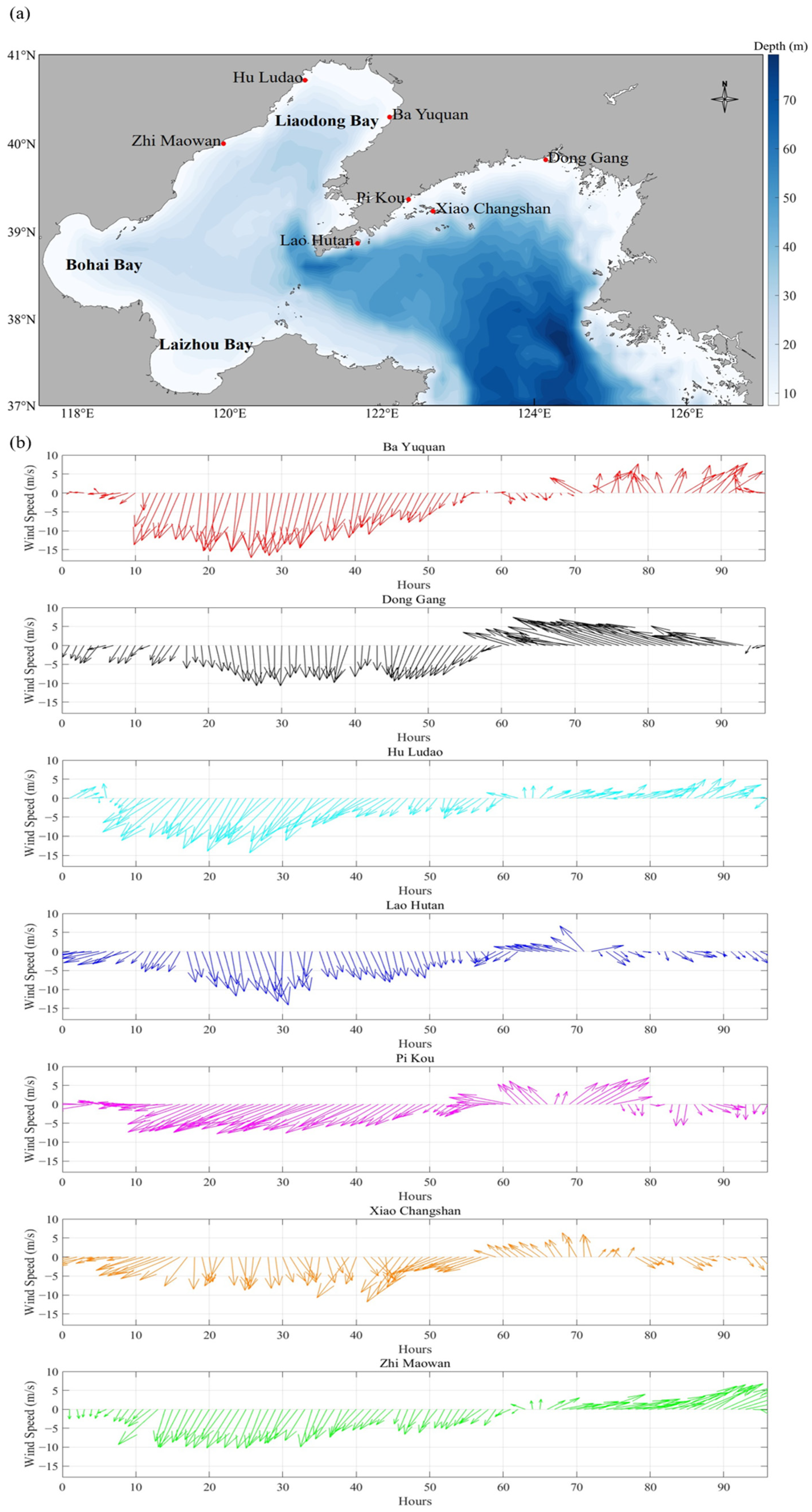
2.1.1. In Situ Measurements
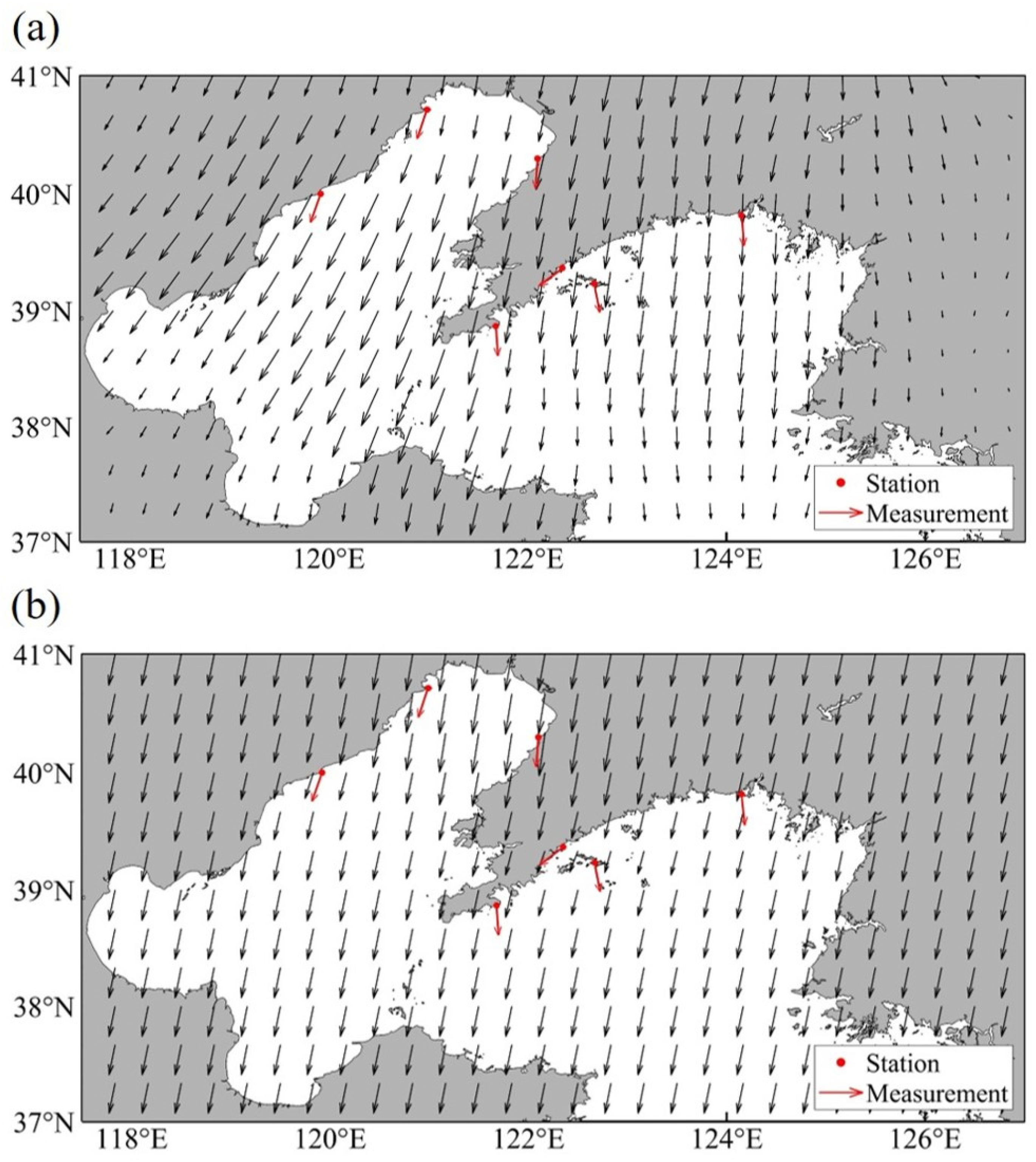
2.1.2. Wind Field
2.2. Methods
2.2.1. Numerical Adjoint Model
2.2.2. Model Construction
3. Results
4. Discussion
5. Conclusions
Author Contributions
Funding
Data Availability Statement
Acknowledgments
Conflicts of Interest
References
- Feng, S.Z. Introduction to Storm Surge; Science Press: Beijing, China, 1982. (In Chinese) [Google Scholar]
- Wang, F.; Liu, X.; Li, Y.; Yu, H.; Wen, M.; Hu, Y. Risk assessment of coastal flooding disaster by storm surge based on Elevation-Area method and hydrodynamic models: Taking Bohai Bay as an example. China Geol. 2024, 7, 494–504. [Google Scholar] [CrossRef]
- Almar, R.; Ranasinghe, R.; Bergsma, E.W.J.; Diaz, H.; Melet, A.; Papa, F.; Vousdoukas, M.; Athanasiou, P.; Dada, O.; Almeida, L.P.; et al. A global analysis of extreme coastal water levels with implications for potential coastal overtopping. Nat. Commun. 2021, 12, 3775. [Google Scholar] [CrossRef]
- Edmonds, D.A.; Caldwell, R.L.; Brondizio, E.S.; Siani, S.M.O. Coastal flooding will disproportionately impact people on river deltas. Nat. Commun. 2020, 11, 4741. [Google Scholar] [CrossRef]
- Zhou, Z.; Yang, S.; Hu, F.; Chen, B.; Shi, X.; Liu, X. Tropical Cyclone Storm Surge-Based Flood Risk Assessment Under Combined Scenarios of High Tides and Sea-Level Rise: A Case Study of Hainan Island, China. Earth’s Future 2024, 12, e2023EF004236. [Google Scholar] [CrossRef]
- Ministry of Natural Resources of China. Ministry of Natural Resources of China: 2023 Chinese Marine Disaster Bulletin; Ministry of Natural Resources of China: Beijing, China, 2024.
- Ministry of Natural Resources of China. Ministry of Natural Resources of China: 2024 Chinese Natural Resources Bulletin; Ministry of Natural Resources of China: Beijing, China, 2025.
- Liang, S.; Zhang, Y.; Fu, X.; Zhu, X. Statistics and numerical simulation on the storm surge in the west coast of the Bohai Sea caused by cold-air-induced northeast strong wind. Mar. Forecast. 2024, 41, 12–21. [Google Scholar]
- Ji, T.; Li, G.; Liu, R. Historical Reconstruction of Storm Surge Activity in the Southeastern Coastal Area of China for the Past 60 Years. Earth Space Sci. 2020, 7, e2019EA001056. [Google Scholar] [CrossRef]
- Su, C.; Sahoo, B.; Mao, M.; Xia, M. Machine Learning Techniques for Predicting Typhoon-Induced Storm Surge Using a Hybrid Wind Field. J. Geophys. Res. Mach. Learn. Comput. 2025, 2, e2024JH000507. [Google Scholar] [CrossRef]
- Shankar, C.G.; Behera, M.R. Improved Wind Drag Formulation for Numerical Storm Wave and Surge Modeling. Dyn. Atmos. Ocean. 2021, 93, 101193. [Google Scholar] [CrossRef]
- Liu, M.; Lv, X. Study on the Drag Coefficient in the Simulation of Storm Surges with Adjoint Method. Oceanol. Limnol. Sin. 2011, 42, 9–19, (In Chinese with English Abstract). [Google Scholar]
- Wróbel-Niedźwiecka, I.; Drozdowska, V.; Piskozub, J. Effect of drag coefficient formula choice on wind stress climatology in the North Atlantic and the European Arctic. Oceanologia 2019, 61, 291–299. [Google Scholar] [CrossRef]
- Wu, J. Wind-Stress coefficients over Sea surface near Neutral Conditions—A Revisit. J. Phys. Oceanogr. 1980, 10, 727–740. [Google Scholar] [CrossRef]
- Smith, S.D.; Banke, E.G. Variation of the sea surface drag coefficient with wind speed. Q. J. R. Meteorol. Soc 1975, 101, 665–673. [Google Scholar] [CrossRef]
- Large, W.G.; Pond, S. Open Ocean Momentum Flux Measurements in Moderate to Strong Winds. J. Phys. Oceanogr. 1981, 11, 324–336. [Google Scholar] [CrossRef]
- Cao, X.; Li, Q.; Xing, C.; Shi, W.; Wu, L.; Gao, J.; Guo, P.; Shi, M. Adaptability of Drag Coefficient to Numerical Simulation of Storm Surge in the Northern South China Sea. Trans. Oceanol. Limnol. 2020, 1, 1–8. [Google Scholar] [CrossRef]
- Li, Q.; Hong, X.; Cao, X.; Yin, L.; Li, P.; Mao, X.; Cao, H. Effects of Different Wind Stress Drag Coefficients on Simulation Accuracy of Typhoon Storm Surge in Beihai Region. J. Hainan Trop. Ocean Univ. 2023, 30, 92–100. [Google Scholar] [CrossRef]
- Wang, X. Test of Influence of Wind Drag Coefficient on Typhoon Storm Surge Simulations. J. Ocean Univ. Qingdao 2001, 31, 640–646, (In Chinese with English Abstract). [Google Scholar]
- Luo, J.; Pan, J.; Yang, Z. Impact of the parameterization scheme about sea surface wind stress drag coefficients on numerical simulation of strom surge. Mar. Forecast. 2011, 28, 15–19, (In Chinese with English Abstract). [Google Scholar]
- Fan, S.; Chu, A.; Jiang, Q. Optimization of reanalysis wind field and its application in the simulation of extratropical storm surge in the Bohai Bay. Mar. Forecast. 2021, 38, 61–68, (In Chinese with English Abstract). [Google Scholar]
- Xiong, J.; Yu, F.; Fu, C.; Dong, J.; Liu, Q. Evaluation and improvement of the ERA5 wind field in typhoon storm surge simulations. Appl. Ocean Res. 2022, 118, 103000. [Google Scholar] [CrossRef]
- Schenkel, B.A.; Hart, R.E. An Examination of Tropical Cyclone Position, Intensity, and Intensity Life Cycle within Atmospheric Reanalysis Datasets. J. Clim. 2012, 25, 3453–3475. [Google Scholar] [CrossRef]
- Liu, F.; Sasaki, J. Hybrid methods combining atmospheric reanalysis data and a parametric typhoon model to hindcast storm surges in Tokyo Bay. Sci. Rep. 2019, 9, 12222. [Google Scholar] [CrossRef] [PubMed]
- Derber, J.C. Variational Four-dimensional Analysis Using Quasi-Geostrophic Constraints. Mon. Weather Rev. 1987, 115, 998–1008. [Google Scholar] [CrossRef]
- Dimet, F.-X.L.; Talagrand, O. Variational algorithms for analysis and assimilation of meteorological observations: Theoretical aspects. Tellus A Dyn. Meterorol. Ocean. 1986, 38A, 97–110. [Google Scholar] [CrossRef]
- Yu, L.; O’Brien, J.J. Variational Estimation of the Wind Stress Drag Coefficient and the Oceanic Eddy Viscosity Profile. J. Phys. Oceanogr. 1991, 21, 709–719. [Google Scholar] [CrossRef]
- Fan, L.; Liu, M.; Chen, H.; Lv, X. Numerical study on the spatially varying drag coefficient in simulation of storm surges employing the adjoint method. Chin. J. Oceanol. Limnol. 2011, 29, 702–717. [Google Scholar] [CrossRef]
- Lionello, P.; Sanna, A.; Elvini, E.; Mufato, R. A data assimilation procedure for operational prediction of storm surge in the northern Adriatic Sea. Cont. Shelf Res. 2006, 26, 539–553. [Google Scholar] [CrossRef]
- Peng, S.; Li, Y.; Xie, L. Adjusting the Wind Stress Drag Coefficient in Storm Surge Forecasting Using an Adjoint Technique. J. Atmos. Ocean. Technol. 2013, 30, 590–608. [Google Scholar] [CrossRef]
- Li, Y.; Peng, S.; Yan, J.; Xie, L. On improving storm surge forecasting using an adjoint optimal technique. Ocean Model. 2013, 72, 185–197. [Google Scholar] [CrossRef]
- Zheng, X.; Mayerle, R.; Wang, Y.; Zhang, H. Study of the wind drag coefficient during the storm Xaver in the German Bight using data assimilation. Dyn. Atmos. Ocean. 2018, 83, 64–74. [Google Scholar] [CrossRef]
- Daosheng, W.; Jicai, Z.; Yaping, W. Estimation of Bottom Friction Coefficient in Multi-Constituent Tidal Models Using the Adjoint Method: Temporal Variations and Spatial Distributions. J. Geophys. Res. Ocean. 2021, 126, e2020JC016949. [Google Scholar] [CrossRef]
- Gao, Y.; Jiao, S.; Fu, K.; Zeng, X.; Lv, X. A Method Using the Huber Function for Inversion of Tidal Open Boundary Conditions of the M2 Constituent in the Bohai and Yellow Seas. J. Atmos. Ocean. Technol. 2023, 40, 113–127. [Google Scholar] [CrossRef]
- Peng, J.; Mao, M.; Xia, M. Dynamics of wave generation and dissipation processes during cold wave events in the Bohai Sea. Estuar. Coast. Shelf Sci. 2023, 280, 108161. [Google Scholar] [CrossRef]
- Wu, S.; Wang, X.; Dai, M.; Song, S.; Ma, Y. The general status of storm surges and the simulation of extratropical storm surges in the Bohai Sea. Acta Oceanol. Sin. 2002, 24, 28–34, (In Chinese with English Abstract). [Google Scholar]
- Zhu, Z.; Wang, Z.; Dong, C.; Yu, M.; Xie, H.; Cao, X.; Han, L.; Qi, J. Physics informed neural network modelling for storm surge forecasting—A case study in the Bohai Sea, China. Coast. Eng. 2025, 197, 104686. [Google Scholar] [CrossRef]
- Mo, D.; Hou, Y.; Li, J.; Liu, Y. Study on the storm surges induced by cold waves in the Northern East China Sea. J. Mar. Syst. 2016, 160, 26–39. [Google Scholar] [CrossRef]
- Lardner, R.W.; Al-Rabeh, A.H.; Gunay, N. Optimal estimation of parameters for a two-dimensional hydrodynamical model of the Arabian Gulf. J. Geophys. Res. 1993, 98, 18229–18242. [Google Scholar] [CrossRef]
- Lv, X.; Wu, Z.; Yin, Z.; Tian, J. Inversion of the Tides with the Open Boundaries of the Bohai, Huanghai and Donghai Seas. J. Ocean Univ. Qingdao 2003, 33, 165–172, (In Chinese with English Abstract). [Google Scholar]
- Lv, X.; Wu, Z.; Gu, Y.; Tian, J. Study on the adjoint method in data assimilation and the related problems. Appl. Math. Mech. 2004, 25, 636–646. [Google Scholar] [CrossRef]
- Krige, D.G. Two-dimensional weighted moving average trend surfaces for ore-evaluation. J. S. Afr. Inst. Min. Metall. 1966, 66, 13–38. [Google Scholar]
- Allard, D.J.-P.; Chilès, P. Delfiner: Geostatistics: Modeling Spatial Uncertainty. Math. Geosci. 2013, 45, 377–380. [Google Scholar] [CrossRef]
- Chen, S.; Guo, J. Spatial interpolation techniques: Their applications in regionalizing climate-change series and associated accuracy evaluation in Northeast China. Geomat. Nat. Hazards Risk 2017, 8, 689–705. [Google Scholar] [CrossRef]
- Smith, S.D. Wind Stress and Heat Flux over the Ocean in Gale Force Winds. J. Phys. Oceanogr. 1980, 10, 709–726. [Google Scholar] [CrossRef]
- Bi, X.; Gao, Z.; Liu, Y.; Liu, F.; Song, Q.; Huang, J.; Huang, H.; Mao, W.; Liu, C. Observed drag coefficients in high winds in the near offshore of the South China Sea. J. Geophys. Res. Atmos. 2015, 120, 6444–6459. [Google Scholar] [CrossRef]
- Takagaki, N.; Komori, S.; Suzuki, N.; Iwano, K.; Kurose, R. Mechanism of drag coefficient saturation at strong wind speeds. Geophys. Res. Lett 2016, 43, 9829–9835. [Google Scholar] [CrossRef]
- Guan, C.; Xie, L. On the Linear Parameterization of Drag Coefficient over Sea Surface. J. Phys. Oceanogr. 2004, 34, 2847–2851. [Google Scholar] [CrossRef]
- Donelan, M.A. On the Decrease of the Oceanic Drag Coefficient in High Winds. J. Geophys. Res. Ocean. 2018, 123, 1485–1501. [Google Scholar] [CrossRef]
- Chen, X.; Hara, T.; Ginis, I. Impact of Shoaling Ocean Surface Waves on Wind Stress and Drag Coefficient in Coastal Waters: 1. Uniform Wind. J. Geophys. Res. Ocean. 2020, 125, e2020JC016222. [Google Scholar] [CrossRef]
- Chen, X.; Ginis, I.; Hara, T. Impact of Shoaling Ocean Surface Waves on Wind Stress and Drag Coefficient in Coastal Waters: 2. Tropical Cyclones. J. Geophys. Res. Ocean. 2020, 125, e2020JC016223. [Google Scholar] [CrossRef]

| Ba Yuquan | Dong Gang | Hu Ludao | Lao Houtan | Pi Kou | Xiao Changshan | Zhi Maowan | |
|---|---|---|---|---|---|---|---|
| Longitude/°E | 122.1 | 124.15 | 120.99 | 121.68 | 122.35 | 122.67 | 119.92 |
| Latitude/°N | 40.3 | 39.817 | 40.715 | 38.867 | 39.367 | 39.233 | 40 |
| Product Name | Spatial Grid Spacing | Time Interval | Website |
|---|---|---|---|
| ASCAT+ERA5 | 0.125° × 0.125° | 1 h | https://data.marine.copernicus.eu/product/WIND_GLO_PHY_L4_MY_012_006/services (accessed on 23 March 2025) |
| ASCAT+ECMWF | 0.125° × 0.125° | 1 h | https://data.marine.copernicus.eu/product/WIND_GLO_PHY_L4_NRT_012_004/services (accessed on 23 March 2025) |
| ERA5 | 0.25° × 0.25° | 1 h | https://cds.climate.copernicus.eu/datasets/reanalysis-era5-single-levels?tab=download (accessed on 23 March 2025) |
| CFSv2 | 0.5° × 0.5° | 1 h | https://www.hycom.org/dataserver/ncep-cfsv2 (accessed on 23 March 2025) |
| MERRA_2 | 0.625° × 0.5° | 1 h | https://gmao.gsfc.nasa.gov/reanalysis/MERRA-2/data_access/ (accessed on 23 March 2025) |
| Product Name | MAE (m/s) |
|---|---|
| ERA5 | 3.79 |
| CFSv2 | 5.75 |
| ASCAT+ERA5 | 5.86 |
| ASCAT+ECMWF | 5.86 |
| MERRA_2 | 6.10 |
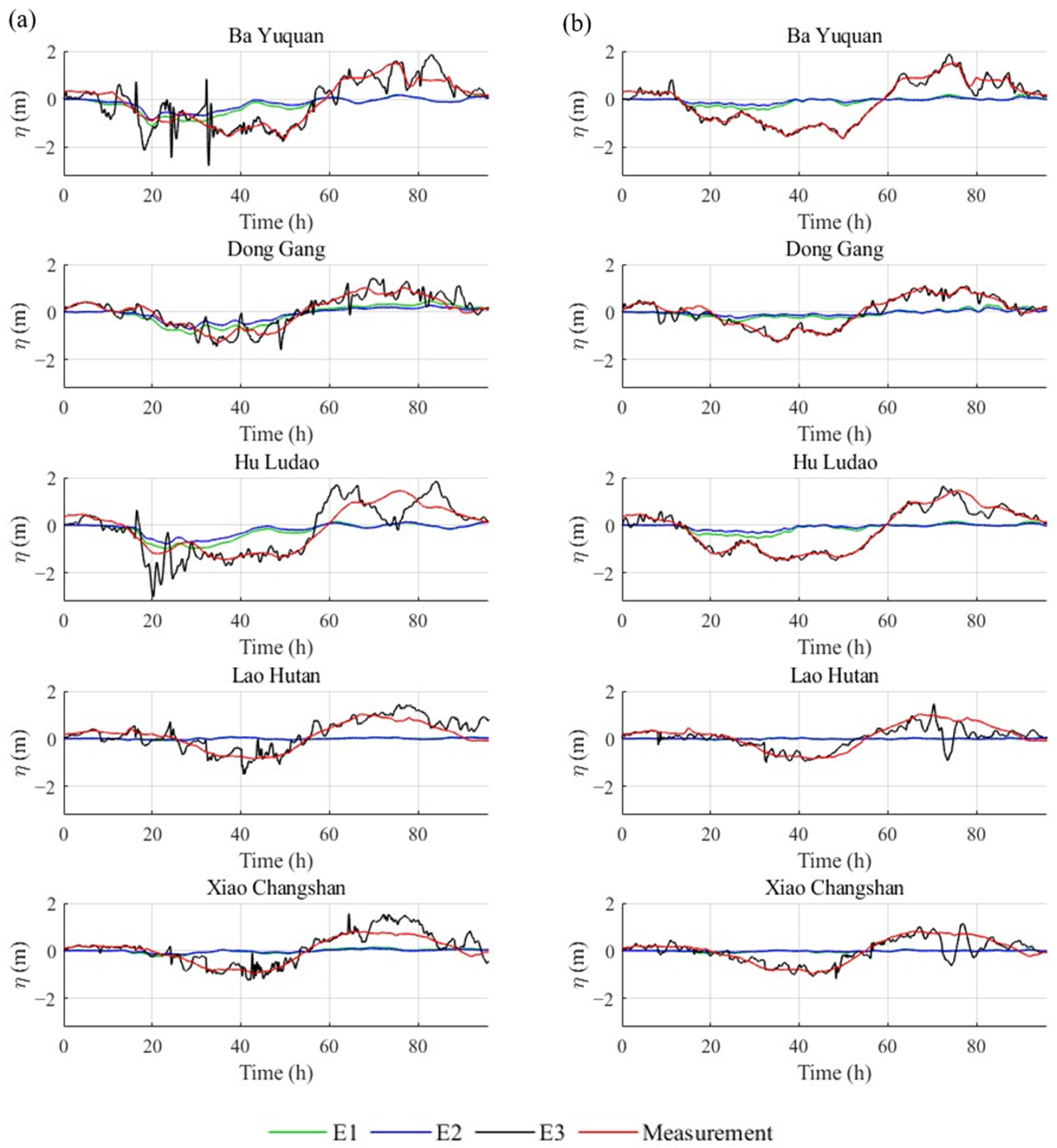
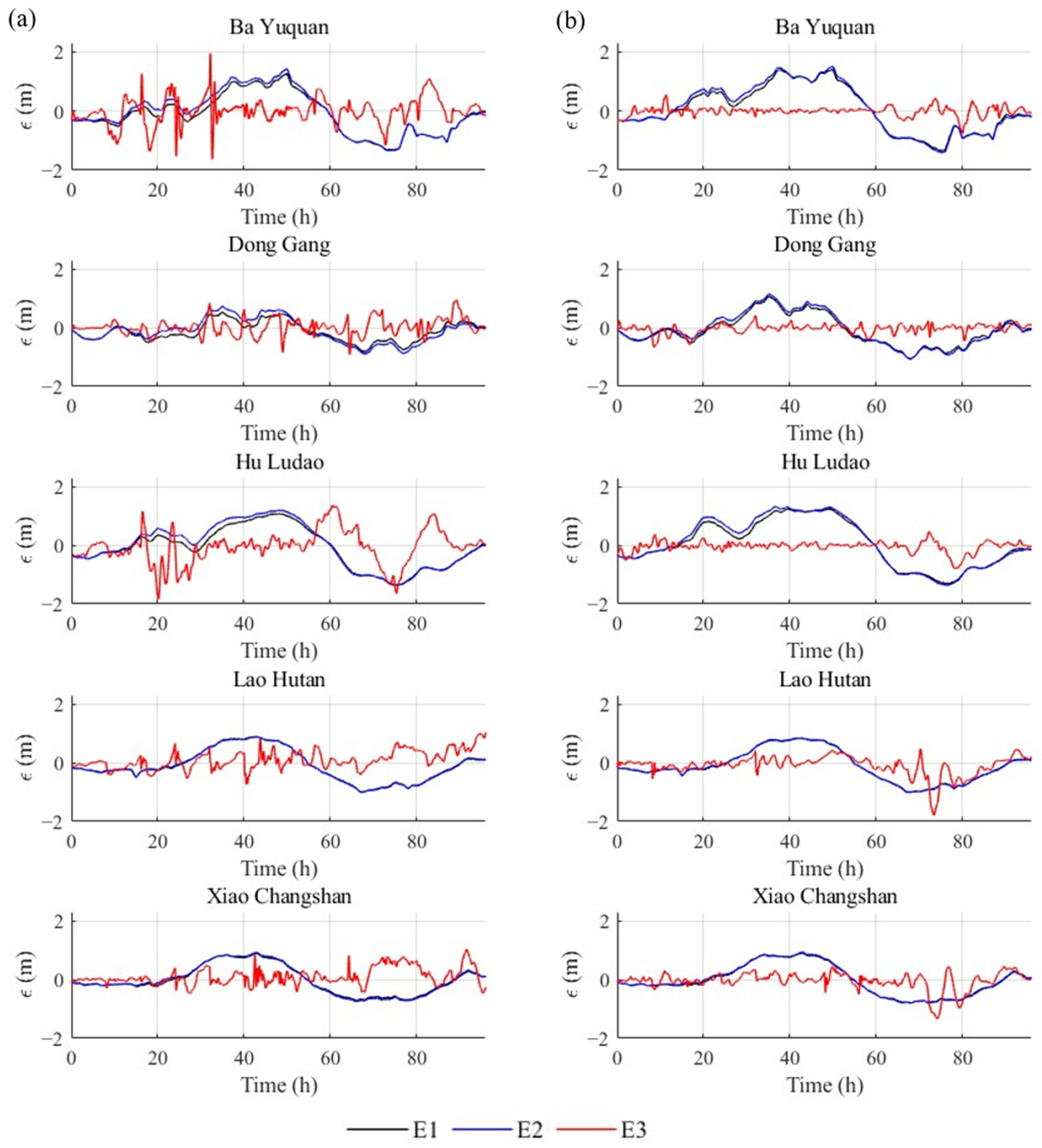
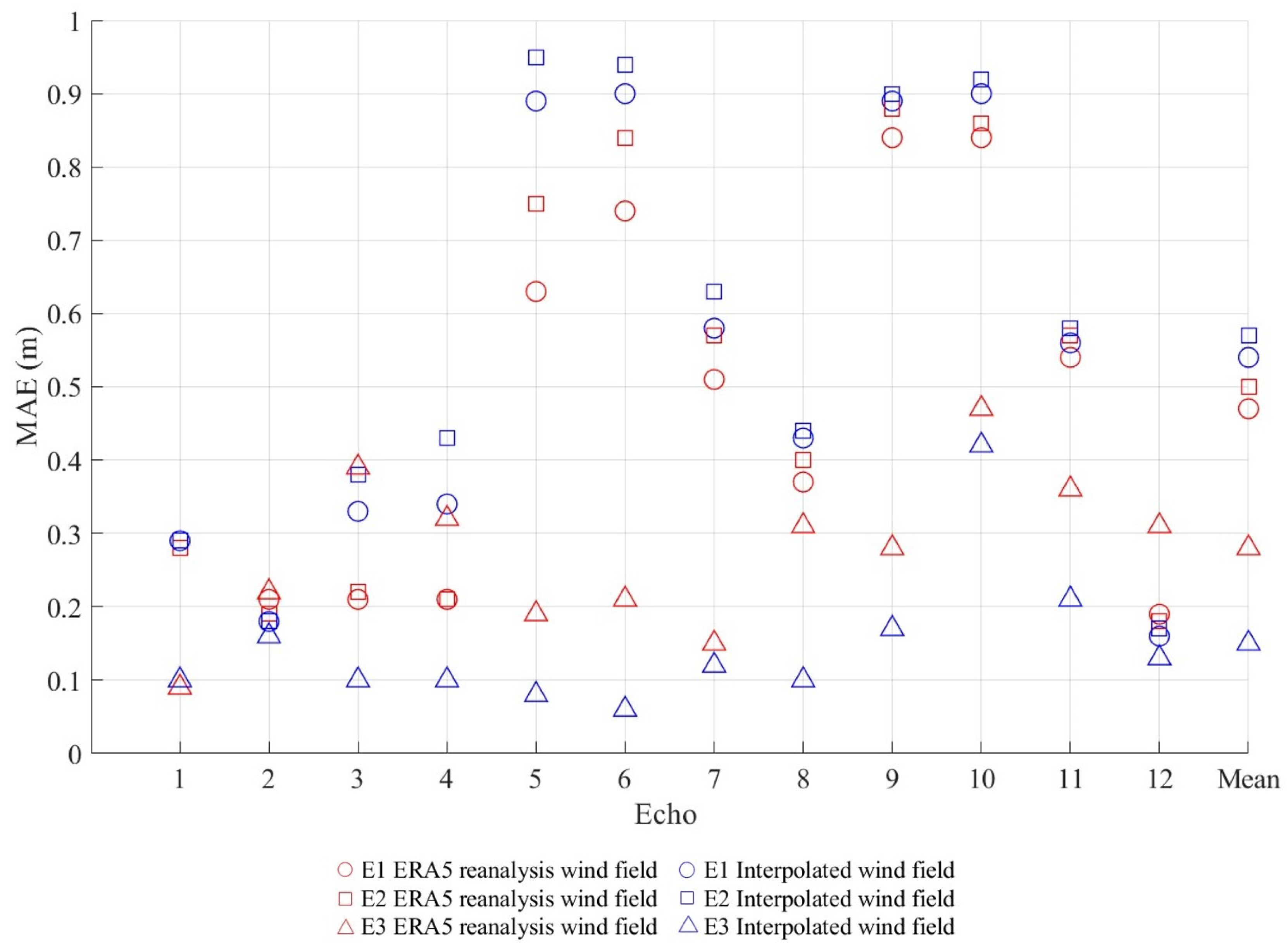
| E1 | E2 | E2(a) | E3 | |||||
|---|---|---|---|---|---|---|---|---|
| EWF | IWF | EWF | IWF | EWF | IWF | EWF | IWF | |
| MAE (m) | 0.46 | 0.54 | 0.50 | 0.57 | 0.51 | 0.57 | 0.28 | 0.15 |
| RMSE (m) | 0.55 | 0.63 | 0.59 | 0.66 | 0.60 | 0.66 | 0.38 | 0.23 |
| R | 0.62 | 0.51 | 0.57 | 0.48 | 0.57 | 0.48 | 0.89 | 0.91 |
Disclaimer/Publisher’s Note: The statements, opinions and data contained in all publications are solely those of the individual author(s) and contributor(s) and not of MDPI and/or the editor(s). MDPI and/or the editor(s) disclaim responsibility for any injury to people or property resulting from any ideas, methods, instructions or products referred to in the content. |
© 2025 by the authors. Licensee MDPI, Basel, Switzerland. This article is an open access article distributed under the terms and conditions of the Creative Commons Attribution (CC BY) license (https://creativecommons.org/licenses/by/4.0/).
Share and Cite
Jiao, L.; Wang, Y.; Jiang, D.; Liu, Q.; Gao, J.; Lv, X. Numerical Simulation of Storm Surge-Induced Water Level Rise in the Bohai Sea with Adjoint Data Assimilation. Remote Sens. 2025, 17, 2054. https://doi.org/10.3390/rs17122054
Jiao L, Wang Y, Jiang D, Liu Q, Gao J, Lv X. Numerical Simulation of Storm Surge-Induced Water Level Rise in the Bohai Sea with Adjoint Data Assimilation. Remote Sensing. 2025; 17(12):2054. https://doi.org/10.3390/rs17122054
Chicago/Turabian StyleJiao, Liqun, Youqi Wang, Dong Jiang, Qingrong Liu, Jing Gao, and Xianqing Lv. 2025. "Numerical Simulation of Storm Surge-Induced Water Level Rise in the Bohai Sea with Adjoint Data Assimilation" Remote Sensing 17, no. 12: 2054. https://doi.org/10.3390/rs17122054
APA StyleJiao, L., Wang, Y., Jiang, D., Liu, Q., Gao, J., & Lv, X. (2025). Numerical Simulation of Storm Surge-Induced Water Level Rise in the Bohai Sea with Adjoint Data Assimilation. Remote Sensing, 17(12), 2054. https://doi.org/10.3390/rs17122054