Article

Quantifying the Drivers of the Spatial Distribution of Urban Surfaces in Bangladesh: A Multi-Method Geospatial Analysis

1
Department of Geography, Florida State University, Tallahassee, FL 32306, USA
2
Department of Geography and Environmental Sustainability, University of Oklahoma, Norman, OK 73019, USA
3
Department of Geosciences, Florida Atlantic University, Boca Raton, FL 33431, USA
*
Author to whom correspondence should be addressed.
Remote Sens. 2025, 17(12), 2050; https://doi.org/10.3390/rs17122050
Submission received: 12 April 2025 / Revised: 4 June 2025 / Accepted: 11 June 2025 / Published: 13 June 2025
(This article belongs to the Special Issue Remote Sensing Measurements of Land Use and Land Cover)

Abstract

Urban expansion threatens sustainable development in densely populated countries like Bangladesh. This study aims to quantitatively identify and evaluate the key drivers influencing the spatial distribution of urban surfaces (SDUS) in Chattogram City, providing insights into urban growth patterns over 30 years. Using Landsat 5 and 9 imageries, the Normalized Difference Built-up Index (NDBI) was computed for 1993 and 2023 to map urban surface changes. A total of 16 geospatial variables representing potential drivers were analyzed. Four statistical and machine learning methods, including GeoDetector, Distributed Random Forest (DRF), global Geographically Weighted Random Forest (GWRF), and local GWRF, were employed to quantify individual and interactive influences on SDUS. The Geodetector analysis identified the central business district (CBD) as the most influential driver of urban surface distribution, with a q statistic of 0.22, followed by river proximity (q = 0.14) and administrative boundaries (q = 0.13). Across all models, CBD consistently ranked as a dominant factor. In the Distributed Random Forest (DRF) model, CBD showed the highest importance score (0.57), followed by coastlines (0.35) and rivers (0.35). The DRF model achieved the highest performance (R2 = 0.612), outperforming the global GWRF (R2 = 0.59) and local GWRF (R2 = 0.529). Although variables like the proximity of administrative location and forests have low individual impacts, they show a stronger coupled influence. This industrial port-based economy expanded, facing challenges of uncontrolled urbanization, poor governance, and environmental issues. Promoting mixed land use planning, decentralizing urban governance, and improving coordination among implementing agencies may better resolve these issues. This work may help planners and policymakers in planning future cities and developing policies to promote sustainable urban growth.

Graphical Abstract

1. Introduction

Humans have always wanted comfort by modifying their surroundings. From early civilization to present cities, a suitable location was decided depending on several physical (e.g., weather conditions and physiography) and anthropogenic (e.g., demographic change, economic prosperity, spatial planning, and infrastructure) causal factors [1,2]. Although available natural resources and their possibility of depletion work as significant pull factors in the early urban establishment phase [3], the physical factors have become less influential than human factors due to technological advancement and infrastructural development with time [4]. The inevitable process of rural-urban conversion occurring at an increasing rate in recent decades significantly affected the functioning of ecosystems, air quality, and urban sustainability [5,6,7,8]. Therefore, it is mandatory to identify what specific drivers influence spatial urban distribution and what the degree of those influences is. Moreover, studying land use and land cover (LULC) change along with its drivers is an increasingly important area to explore in the domain of urban science and applied geography.
Changes in LULC due to human activities are currently occurring faster in developing countries than in the developed world [5]. Due to the tendency of poor people to urbanize faster, growth occurs haphazardly in developing countries [9,10]. Bangladesh has experienced rapid urban population growth in recent decades as a developing country. Urban populations were 14.1 million in 1981, 31.1 million in 2001, and 58 million in 2022 [5,11]. According to the Bangladesh Bureau of Statistics [11], the economically active population (aged above 15) has risen from 13.3 (12.4 employed) million in 2010 to 18.47 (17.69 employed) million in 2022 in the urban areas. Among the employed urban population, 3.3% are in agriculture, 8.2% in industry, 16.4% in the service sector, and the rest are informal [11]. The high amount of informally occupied labor force is the low-income group with low living standards. High migrant pressure and increasing demand for low-cost housing cause more establishment of densified residences and slums. These dynamics of need and fulfillment vary across and within cities, resulting in spatial inequalities of opportunities and facilities and significantly impacting spatial urban distribution.
Remote Sensing and GIS have the capability of capturing spatial dynamism at different scales. Numerous satellite remote-sensing techniques have been developed to assess variations in spatial urban distribution and associated drivers using satellite data [12,13]. Indices such as NDBI, NDBaI, NDVI, and NDWI derived from multi-spectral bands have been deployed widely to extract biophysical information about the land surface [14]. These indices have the advantage of usage. For instance, NDVI extracts vegetation properties properly, but shows a lack in the proper identification of built surfaces. Although NDVI values below 0 represent water surface, they often show discrepancies in identifying water surface, especially near vegetated surfaces or vegetated wetlands. In that, NDWI works as a savior to extract the water surface properly. However, none of the indices properly addresses the concern of this study focusing on urban areas. NDBI is one of the most used indices for extracting urban features, and it marks out built-up areas significantly; therefore, it was chosen for this research to represent urban surfaces. In this study, urban surfaces refer to built-up or impervious areas such as roads, buildings, and other constructed features. These surfaces are represented using continuous NDBI values, which serve as a proxy for the intensity and distribution of urban development. Ghosh et al. [15] reported an overall accuracy of 76.45% and a kappa coefficient of 0.57 using NDBI for mapping built-up areas in Rajarhat Block, India, surpassing other commonly used indices such as the Urban Index (UI) and the Normalized Difference Bareness Index (NDBaI). Similarly, Kebede et al. [16] demonstrated that NDBI achieved a spectral discrimination index (SDI) up to 1.26 and accuracy up to 94% across multiple years in Addis Ababa, affirming its robustness across temporal scales and heterogeneous urban textures. Indices such as the Urban Index (UI) and the Band Ratio for Built-up Area (BRBA) utilize comparable spectral band combinations and can occasionally offer better discrimination in transitional urban–rural landscapes [17]. However, the Built-up Area Extraction Index (BAEI) has demonstrated weak reliability in distinguishing built-up features from other land cover types [16], rendering it unsuitable for complex urban environments like Chattogram. In their evaluation, although BRBA was able to enhance features like roads and exposed soil, it struggled to differentiate vegetated areas from built-up surfaces due to spectral confusion. Similarly, the Modified Built-up Index (MBI) exhibited only moderate effectiveness in separating impervious surfaces from surrounding land covers.
Moreover, different powerful methods like Geodetector, GWR, and Machine Learning are used in geospatial research for understanding the influence of spatial variables and modeling. Geodetector analyzes spatial stratified heterogeneity (SSH) among different GIS/RS layers to understand which independent variables influence the change most and which factors have the most combined impact [2,18,19]. The SSH specifically arises when spatial variation is organized into distinct strata or zones, where within-stratum variation is smaller compared to between-stratum variation [19,20]. These strata may represent administrative boundaries, ecological zones, or spatial distributions of traits such as population density, climate, soil types, or LULC patterns. The existence of SSH suggests that unique processes or mechanisms may dominate within each stratum [21], which can influence spatial analyses. Failing to account for SSH in global statistical models can lead to significant issues, such as aggregation bias and ecological fallacies, where global models mask underlying localized processes or interactions [22,23]. To detect such geographical differences, the GeoDetector modeling technique, which was first presented by Wang et al. [20], has become widely popular and used by researchers in different areas such as urban growth, vegetation dynamics [2,24,25]. Moreover, DRF was expanded upon the Random Forest (RF) framework, which is designed for efficient and scalable prediction in high-dimensional and large-scale datasets [26,27]. DRF constructs an ensemble of decision trees either for classification or regression rather than relying on a single tree model. Each tree in the ensemble is developed using a random subset of the input data, both in terms of rows (observations) and columns (features), and each tree is the individual weak learner. As the number of trees increases, the overall model variance tends to decrease, enhancing stability. The final output is obtained by aggregating the predictions from all trees using majority voting for classification and averaging for regression. The GWRF model extends the capabilities of Random Forest by incorporating spatial heterogeneity in the relationships between the dependent variable and its predictors. Unlike the traditional RF model, which is aspatial, GWRF constructs localized models for each observation in the dataset, considering spatial proximity. The foundational concept is inspired by Geographically Weighted Regression (GWR) [28], where we move from global to local calculation. This enables the model to capture non-stationary relationships that vary across space, providing both predictive accuracy and explanatory power [29]. Furthermore, because the Random Forest algorithm performs well in high-dimensional situations, this model is a good choice for our study with a lot of predictors.
Chattogram City’s physical form has undergone drastic changes in recent decades due to its vast expansion in almost all directions because of internal transformations [30]. Urban expansion in ecologically sensitive and topographically complex regions like Chattogram City frequently unfolds in a fragmented and largely unregulated manner. This pattern of growth poses significant challenges for sustainable land use planning, disaster risk reduction, and long-term environmental stewardship. As Chattogram continues to develop rapidly, often in response to economic pressures and population growth, the city’s spatial trajectory stresses the urgent need for a deeper understanding of the forces shaping its urban form. This study is motivated by the imperative to investigate the key determinants influencing the spatial configuration of urban development in Chattogram, with the broader aim of informing policy frameworks that support more resilient and sustainable urban growth. In this area, several studies have been published analyzing satellite sensor data over different spatiotemporal scales [31,32,33,34,35,36,37,38]. Hassan & Nazem [33] documented rapid urban growth in the study area with an average increasing rate of 17.5% per year, increasing the risk of vegetated hills encroachment. Rahman [35] studied gentrification in Chattogram City and discussed how it works as a process of urban development. Samad et al. [38] studied rapid urban growth and discussed its impact on the environment. Several studies also concluded that the intense urbanization led to a rise in land surface temperature, impacting human thermal comfort as the highest temperature remains in urban areas [31,34,37]. Hasan et al. [32] observed significant environmental decline in the region, identifying key ecological issues, including extensive deforestation, loss of biodiversity, soil erosion, and disruptions to aquatic carbon sequestration. Collectively, these studies focused on identifying LULC classes, their spatiotemporal changes, and their impact on land surface temperature. They also outlined the critical role of remote sensing in understanding spatiotemporal dynamics in urban areas. But there remains a crucial gap in identifying and quantifying the spatial drivers that shape the distribution of urban surfaces. No prior studies have conducted data-driven analysis to understand the factors of the spatial urban distribution in the study area.
The main purpose of this research is to develop an understanding of significant driving forces shaping the SDUS in Chattogram City. Primarily, Landsat-derived NDBI provided information on urbanized surfaces across the city. Afterward, this study addresses the research gap by using an integrated, comparative approach involving GeoDetector, DRF, and both global and local GWRF models to uncover the most influential factors and their spatial heterogeneity. The goal is to move beyond descriptive analyses and provide deeper insights that can inform targeted, spatially responsive urban planning, particularly in critical areas such as future development planning, industrial zoning, and resource allocation, in one of Bangladesh’s most ecologically sensitive urban regions.

2. Materials and Methods
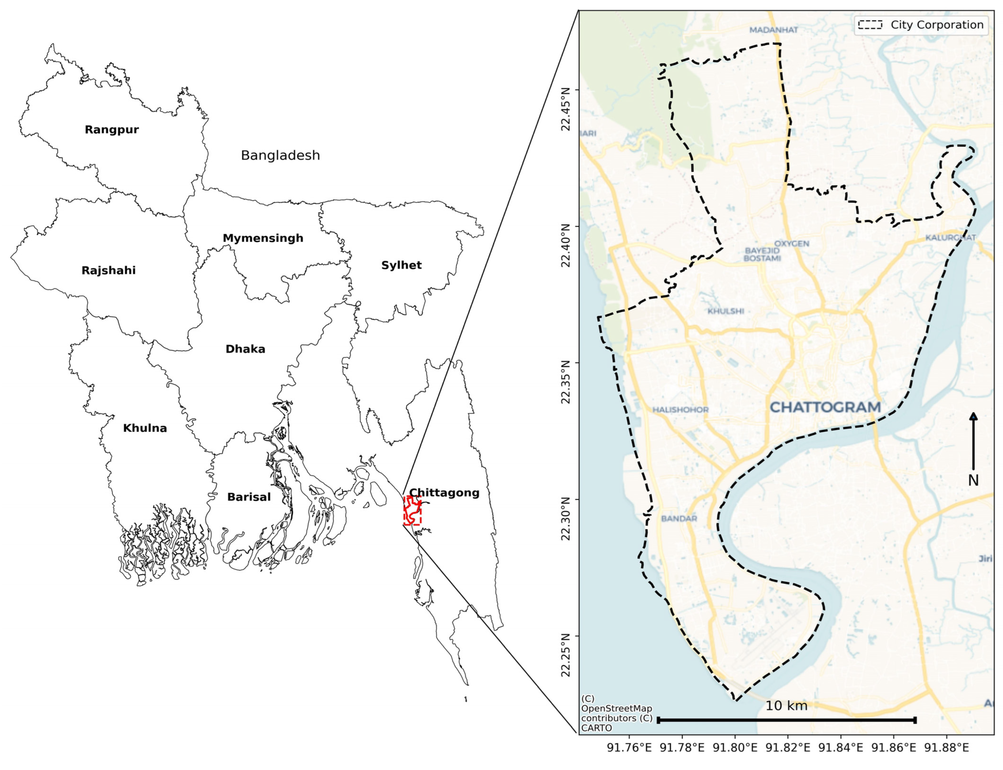
2.1. Study Area

Chattogram City is situated between 22°13′ and 22°28′N Latitude and between 91°44′ and 91°53′E Longitude, as shown in Figure 1. Currently, Chattogram City has an approximate total population of 6 million which was around 2.2 million in 1990 [39,40]. Having good transportation access through highways, railways, waterways, and airways, Chattogram City is the second largest in the country, and is one of Bangladesh’s most prominent trade hubs and commercial capitals [41]. Its economy is primarily driven by industrial and manufacturing activities, with garment manufacturing being the most significant employment source [40]. With its enormous population and natural resources, the city generates various industrial items such as cement, fertilizers, and chemicals as well as a large share of national textile exports.
The topography and physiography of the city are distinctive in Bangladesh. It is combined with undulating low hillocks and flood plains of the Halda and Karnafuli rivers. The prominent Piedmont and valley topography jointly occupies approximately 16% of the city area, with the remaining mainly covering flat alluvial plains [42]. The plains have an average elevation of around 7 m above sea level, whereas the northern highlands have elevations ranging from 30 to 140 m above sea level (Figure 2n). Having a tropical monsoon climate, the city has hot and humid summers with moderately cold winters. The normal monthly temperature ranges from 19.8 °C to 28.6 °C, and annual rainfall ranges from 3200 to 3500 mm in the region [43].

2.2. Data Characteristics

Primarily, Landsat Collection-2 Level-2 data of OLI-2 sensor (CLOUD_COVER_LAND = 7.70), TM sensor (CLOUD_COVER_LAND = 0.00), and SRTM digital elevation model (DEM) data were acquired from the USGS website. Along with that, 5 major types of spatial layers, such as natural features, topographic features (prepared using DEM), public services and amenities, economic and commercial centers, and infrastructure, were collected from different sources (Table 1).

2.3. Methods

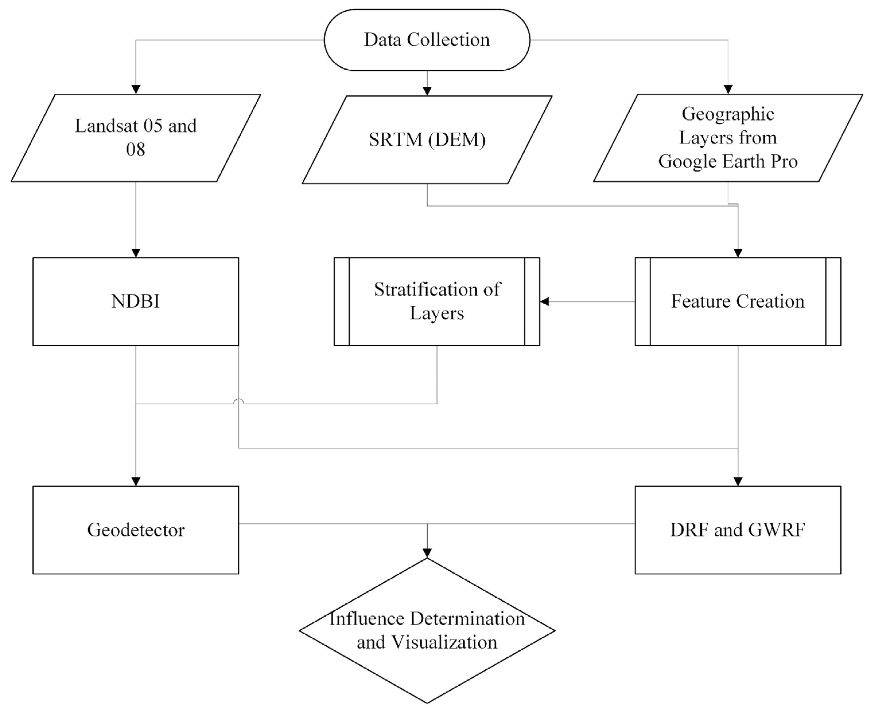
2.3.1. Data Processing

Landsat Collection 2 Level 2 data comes analysis ready and, therefore, does not require any correction. Topographic variables (elevation and slope) were derived from digital elevation model (DEM) data. Euclidean distance was measured from the collected GIS layers for other variables to create continuous raster layers for Geodetector analysis. All the processed layers are shown in Figure 2. Prior to stratification for GeoDetector, we performed Pearson correlation analysis between the continuous NDBI values and the continuous proximity values of driving factors. This helped identify the direction of association (positive or negative) between urban surface distribution and each factor (e.g., distance from forest or CBD), thereby supporting interpretation of variable influence. All the steps followed in this research can be seen in Figure 3.

2.3.2. Index-Based Urban Surface Determination

To date, a variety of indices have been developed utilizing multispectral bands to study urban areas. This study utilized the NDBI technique developed by Zha et al. [45] in Equation (1) to understand SDUS in Chattogram City. Utilizing indices is quite challenging to extract urban pixel information. Easy-to-use methods utilizing multispectral bands often comprise accuracy, whereas complex indexing with added layers, such as night-time light, improves precision. NDBI was selected due to its simplicity, computational efficiency, and proven effectiveness in delineating built-up surfaces. NDBI is particularly advantageous in urban areas where the spectral contrast between built-up and vegetated surfaces is pronounced. One of the primary strengths of NDBI lies in its use of the shortwave infrared (SWIR) and near-infrared (NIR) bands, which capitalize on the higher reflectance of built-up surfaces in the SWIR region and the lower reflectance in the NIR. This spectral contrast enables the effective discrimination of impervious surfaces from vegetation and other land covers [17,45], resulting in consistently high mapping accuracy. However, a major challenge is to distinguish urban pixels from the exposed soil surface and beach sand, considering the complex surface of coastal Chattogram City. However, we selected the Landsat image from April because of the crop availability to reduce the effect of exposed soil from agricultural land. In addition, we extracted the beach sand area through manual digitization and removed such areas to have less conflict with urban pixels.
N D B I = ( S W I R N I R ) ( S W I R + N I R   )  

2.3.3. Geodetector

To identify and quantify the driving factors influencing SDUS in Chattogram City, we utilized the GeoDetector model, a robust statistical framework designed to measure SSH and determine the strength of associations between spatial variables and dependent outcomes. This model is particularly well suited for analyzing the non-linear and interactive relationships between natural, socioeconomic, and built-environment factors [20,46], which are key in urban studies and have been used in this model. In this model, it is assumed that if there is a significant relationship between the independent variables X and Y, their spatial distributions should exhibit comparability [20]. In this study, we employed the factor detector and interaction detector functions from the GD package to analyze these relationships [47]. To detect spatial heterogeneity (SH), the factor detector was used to measure the explanatory power of each independent variable (Table 1) on urban expansion. The explanatory power of a factor is quantified by the q-statistic, which ranges from 0 to 1 [48]. The value of q = 1 determines that the dependent and independent variables show a similar spatial distribution in geographical space, as well as the value of q = 0 shows alternative results [49]. It is defined as Equation (2):
q = 1 h = 1 L N h σ h 2 N σ 2
where Nh and σh2 represent the sample size and variance within stratum h, respectively. N and σ2 denote the total sample size and global variance. A higher q-value indicates a stronger influence of the factor on urban expansion [20].
For validating the results of Geodetector, three stratification methods were used on the independent variables to classify them into 5 categories. To ensure the reliability and robustness of the Geodetector results, we compared output from Equal Interval, Quantile, and Fisher–Jenks (Natural Breaks). The Fisher–Jenks method was selected for final stratification for this study. It is particularly appropriate for continuous or ratio–scale spatial variables like proximity distances, elevation, and aspect-derived measures because it identifies natural groupings in the data by minimizing within-class variance and maximizing between-class differences [50].
To assess whether the interaction between two factors enhances, weakens, or has no effect on urban expansion, the interaction detector was applied. This step examines whether the two factors combined explain more spatial variance than expected from their individual effects. Interactions can be categorized as linear enhancement, non-linear enhancement, or weakening [46].

2.3.4. Distributional Random Forest (DRF)

For this study, a global random forest regression model was implemented using the Distributed Random Forest (DRF) algorithm, a robust ensemble learning method for regression and classification tasks. For running this model, all spatial layers were integrated into a unified shapefile, and associated metrics were extracted as Euclidean distances. The final dataset included 14,986 observations randomly selected from the entire dataset for the global and local machine learning (ML) models. All the covariates were transformed into numeric variables for further analysis. This numeric sample dataset was then randomly split into training (60%), validation (20%), and testing (20%) sets. All covariates were standardized using z-score normalization to improve model convergence and interpretability.
The DRF model was trained using the h2o machine-learning framework [27]. We performed a random grid search over 200 combinations of hyperparameters to identify the optimal set of hyperparameters, including the number of trees (10–5000), maximum tree depth (10–50), and sample rates (0.7–10). During this hyperparameter tuning, early stopping is applied with a fixed stopping tolerance of 0.001 and a patience of 2 rounds. This was applied to prevent overfitting and improve computational efficiency. Moreover, we leveraged a 10-fold cross-validation approach to systematically explore all possible hyperparameter combinations and select the best-performing configuration. The best-performing DRF model was selected based on lower RMSE in the validation data. The best-performing model consisted of 194 trees with a maximum depth of 20 and full sample rate (1.0). This model is then used to predict urban expansion for the year 2023. Model performance was evaluated using out-of-bag (OOB) error forest metrics, which provide unbiased estimates of prediction error [51]. Additionally, permutation-based feature importance was calculated using the VIP package [52] with 10 Monte Carlo simulations, where variables are ranked based on their contribution to reducing the residual variance during tree splits.

2.3.5. Geographically Weighted Random Forest (GWRF)

To account for spatial heterogeneity in the predictors of urban spatial distribution (SUDS), we implemented the Geographically Weighted Random Forest (GWRF) model using the SpatialML package in R [53]. The GWRF combines the predictive power of ensemble learning (via Random Forest) with the spatial sensitivity of Geographically Weighted Regression (GWR), making it suitable for capturing localized patterns across urban environments [29]. Random Forest (RF) is a widely used ensemble machine learning algorithm known for its robustness in handling complex, non-linear relationships and high-dimensional data [26]. It operates by constructing a multitude of decision trees during training and aggregating their predictions either by majority vote (classification) or by averaging (regression). Each tree is trained on a bootstrap sample of the data, and at each node, a random subset of predictors is considered for splitting. This dual randomness through both data sampling and feature selection introduces diversity among the trees and helps mitigate overfitting. While RF assumes spatial stationarity in relationships, many urban and environmental processes exhibit spatial heterogeneity, such as the influence of predictors may vary across space. To capture such local variability, Geographically Weighted Random Forest (GWRF) extends the RF framework by incorporating the principles of spatial weighting from Geographically Weighted Regression (GWR) [28,29]. GWRF enables the exploration of spatial variation in the relationships between a target variable and its predictors. It accounts for the fact that predictor effects may differ across locations. To address this spatial heterogeneity, GWRF constructs local models by integrating a spatial weighting scheme typically through a kernel function with the Random Forest algorithm, allowing each location to be influenced more strongly by its nearby observations.
We trained the GWRF model with the same dataset utilized for the global model. Coordinates (X, Y) were provided for each observation to compute spatial weighting. The adaptive kernel approach was applied to define the neighborhood for each local model, with bandwidth determined through cross-validation to minimize prediction error. We used an adaptive bi-square kernel with a bandwidth of 500. The optimal bandwidth was determined with an exhaustive approach using the grf.bw() function to balance model performance and spatial smoothness. Each local model was trained with 200 trees and a randomly selected subset of two predictors. The model outputs both global and local variable importance, residual diagnostics, and R2 scores. Local predictions were generated separately for validation and test datasets, and model performance was assessed using the same error metrics as global. Furthermore, Local feature importance scores were computed for each predictor to analyze spatial variability in their influence on the target variable.

3. Results

3.1. Validation of the Results

By comparing the results of three stratification methods, we can see almost identical outputs with a maximum standard deviation of 0.03 (Table A1). Among the three methods, Fisher–Jenks more effectively captured the natural spatial groupings, supporting a more meaningful interpretation of land use change drivers.
For DRF and GWRF model validation, cross-validation metrics showed that the non-spatial DRF model outperformed both the global and local GWRF models, achieving the lowest RMSE (0.622), MAE (0.473), and highest R2 (0.612) (Table A2). While the Global GWRF model showed modest improvement by incorporating spatial structure, the Local GWRF model underperformed, suggesting that hyper-local spatial modeling may not generalize effectively across complex urban landscapes like Chattogram. However, rankings from all the methods were similar in capturing major variables that influenced SDUS.

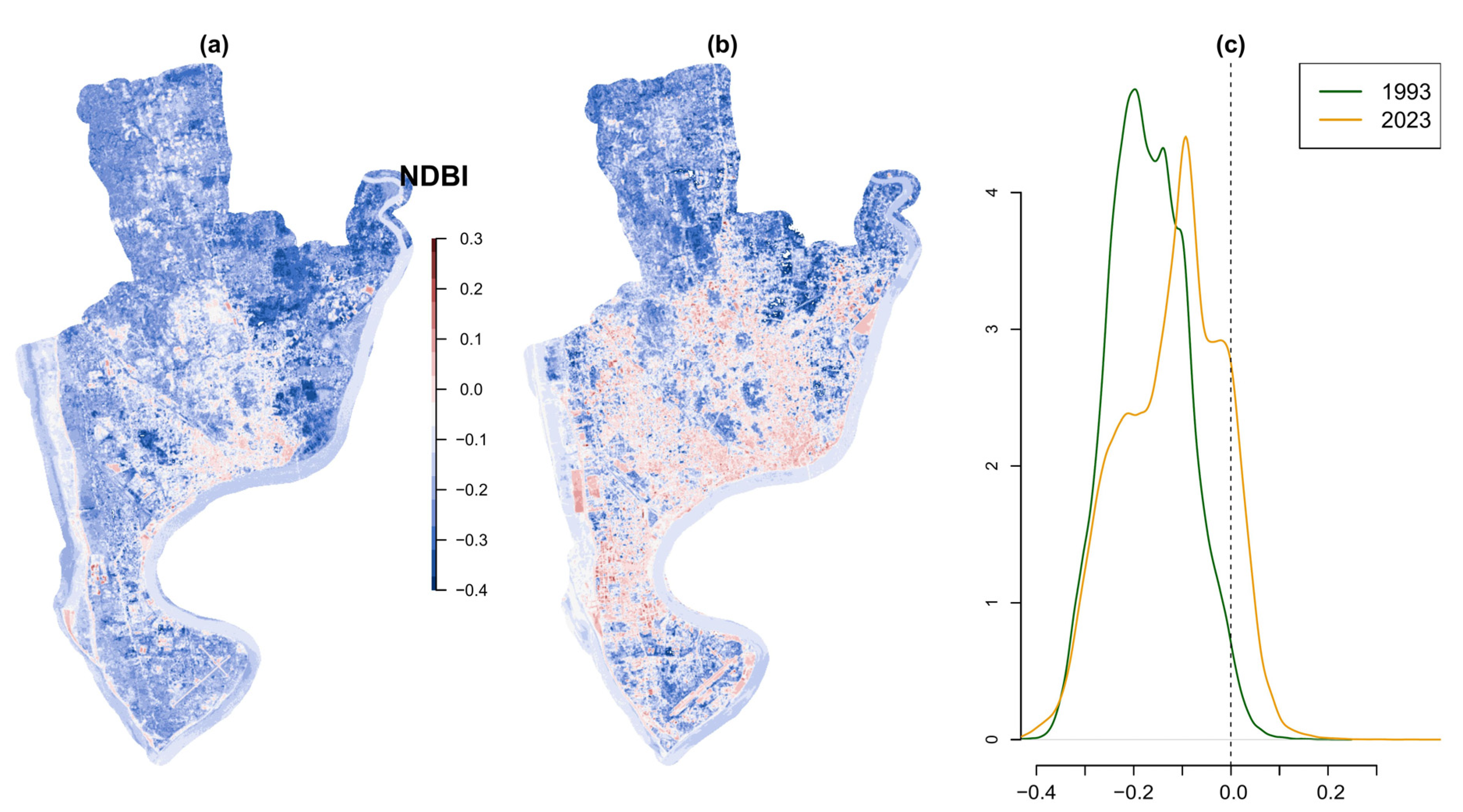
3.2. Spatial Distribution of Urban Surface and Temporal Change

Figure 4a,b display the spatial distribution of NDBI values for the years 1993 and 2023, respectively, with north oriented at the top of each map. The NDBI values range from −0.4 to +0.3, where positive values represent built-up or impervious surfaces (e.g., concrete, rooftops), while negative values correspond to vegetated, water-covered, or otherwise non-urban land cover types. In 1993 (Figure 4a), the area is predominantly characterized by negative NDBI values, indicating a largely vegetated or undeveloped landscape. By 2023 (Figure 4b), there is a notable increase in positive NDBI values, signifying a substantial expansion of built-up land. This urban growth is particularly concentrated in the central and southern parts of the study area, with built-up development also radiating outward toward the north and northwest, mostly. The spatial pattern suggests a clear directional trend of urbanization moving from the southern core toward the northern and southwest peripheral zones, possibly reflecting the influence of transportation infrastructure development (north and northwest) and industrial zones (southwest). Figure 4c presents kernel density estimates of NDBI values for 1993 and 2023, offering a statistical perspective on the temporal dynamics of land cover change. The 1993 curve is left-skewed with a peak in the negative NDBI range, indicating a landscape dominated by non-built-up surfaces. In contrast, the 2023 curve shifts rightward and flattens, reflecting both an increase in built-up intensity and greater spatial heterogeneity in urban development. The vertical dashed line at NDBI = 0 marks the transition between non-built and built environments, with the shift across this threshold serving as quantitative evidence of extensive urban transformation over the past three decades. Collectively, this figure illustrates both the spatial extent and directional tendency of urbanization, confirming a clear trend of land conversion and urban intensification from 1993 to 2023.

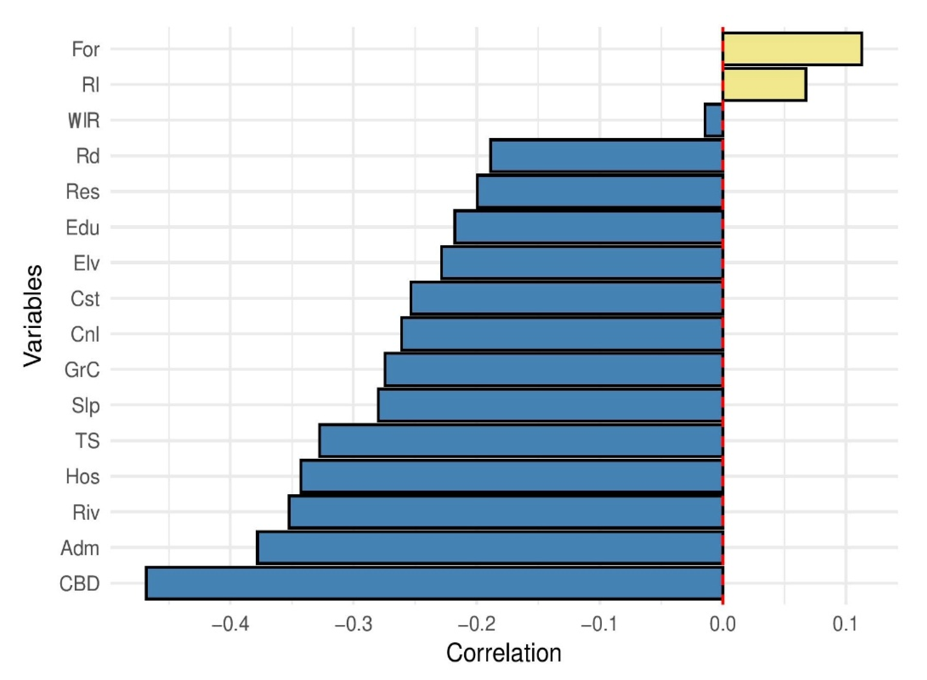
3.3. The Influence and Direction of Individual Factors

The factors were analyzed using four different methods, evaluating the influence of these variables in explaining the SDUS (Table 2). The Geodetector model was employed to quantify the spatial stratified heterogeneity of explanatory variables influencing land use change across Chattogram city. Using the Fisher–Jenks (Natural Breaks) method for discretization, Geodetector analysis showed that the CBD has the highest significant spatial influence with a q-statistic of 0.22, followed by river proximity (q = 0.14) and administrative centers (q = 0.13). These results suggest that economic and administrative accessibility are the most spatially influential factors shaping land use dynamics in the study area. Variables such as hospitals (q = 0.11), transport stations (q = 0.10), and elevation and slope (both q = 0.08) also demonstrated moderate to low spatial influence.
To validate and complement the spatial explanatory analysis, three machine learning models were employed: Global Geographically Weighted Random Forest (Global GWRF), Local GWRF, and a non-spatial Distributed Random Forest (DRF). In the Global GWRF model, the variable importance rankings closely mirrored those from GeoDetector. CBD emerged as the most significant predictor (importance score = 1846.28), followed by forest cover (1522.42) and river proximity (1135.10). In contrast, the Local GWRF model assigned the highest importance to forest cover (26.34), river proximity (22.83), and coastline proximity (22.16), while CBD’s importance dropped to fifth (21.18). This indicates that local variations in spatial context may reduce the predictive strength of centralized variables like CBD. Additionally, forest cover may exert a stronger influence in hilly settlements near forests, which are ecologically sensitive areas. The non-spatial DRF model reaffirmed the significance of CBD (importance = 0.57), river proximity (0.35), and coastline (0.35), suggesting that even without accounting for spatial coordinates, these factors play dominant roles in explaining land use patterns. Administrative centers (0.31), forest (0.34), and residential services (0.30) also had notable importance.
Considering the direction of influence, Figure 5 shows that all the variables, except distance from forest and rail, positively correlate with NDBI. This correlation indicates that the built-up areas are more congested in the nearest areas, and with increasing distance, the urban pixel density reduces. Therefore, high urban areas are distant from the forest and railways.
To summarize, CBD emerges as the most influential factor across all the methods. Apart from CBD, river proximity, coasts, and administrative centers consistently ranked among the top predictors, reinforcing their central role in urban land transformation. While spatial models like GWRF provide deeper insights into geographic variation, the GeoDetector and DRF models offered a more stable and interpretable view of variable importance. The validation process confirmed that the Fisher–Jenks stratification method for GeoDetector produced results closely aligned with those from machine learning models, lending credibility to the spatial explanatory findings.

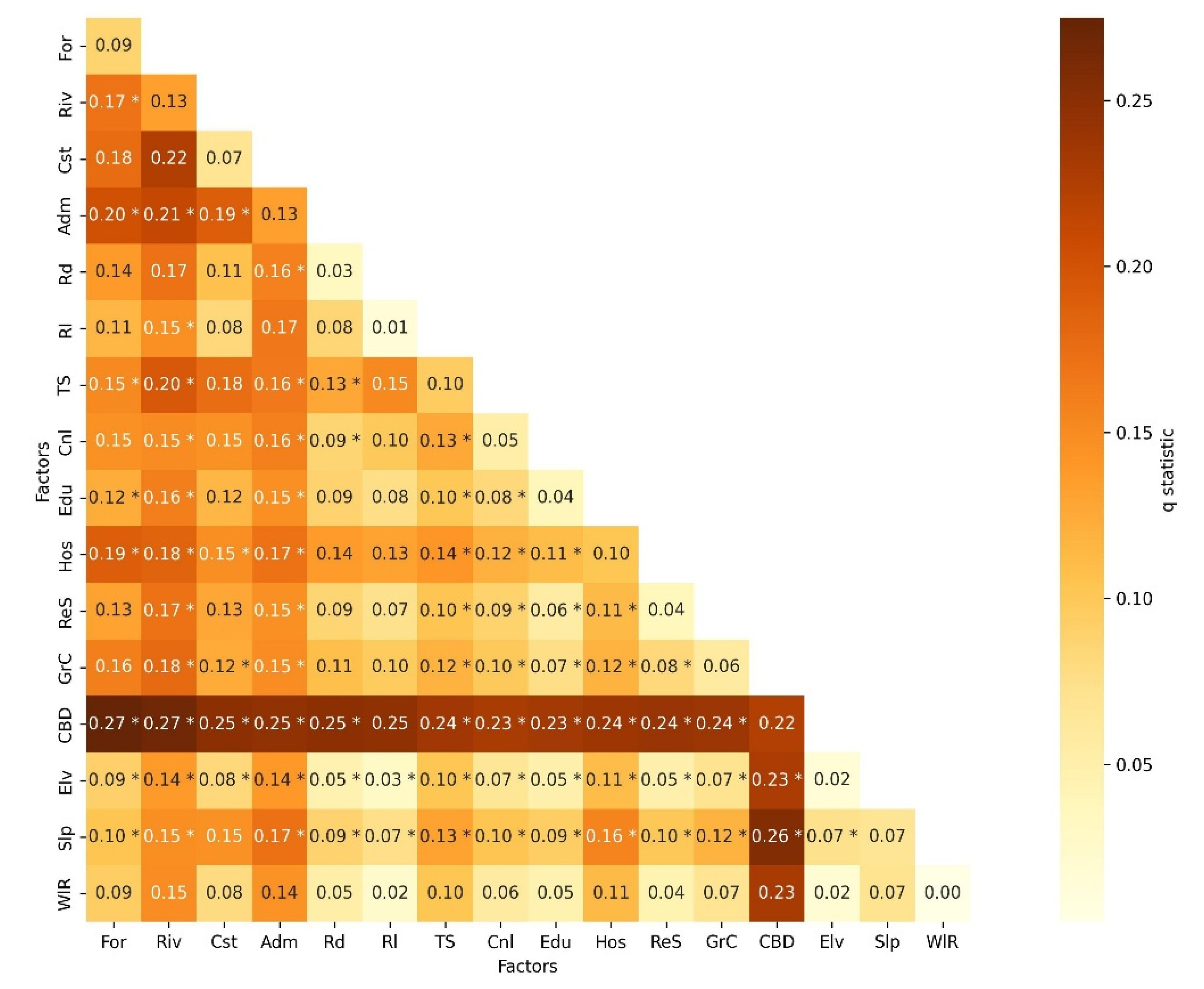
3.4. Combined Influence of Factors

Figure 6 illustrates that strong mutual influence can be seen in the CBD interacting with all the variables, probably because of its high individual importance, indicating the central role in influencing urban form. This combined influence of CBD with other variables can be described as bi-linear, except that the railways and waterlogging risks show non-linear complex interaction. Significant co-influence of CBD can be seen with variables such as forests, rivers, slopes, coast, administrative buildings, roads, and railways. These high q-values, especially with bi-linear enhancements (*), indicate that proximity to central economic hubs, accessibility infrastructure, and government institutions jointly drive urban expansion patterns. Similarly, other factors such as slope (Slp), educational institutions (Edu), and transportation stations (TS) demonstrate moderate interaction effects with built-up patterns, particularly when coupled with CBD, roads, and administrative zones, suggesting that access to governance, transportation, and economic centers acts as a magnet for urban expansion. Apart from CBD coupling with other variables from Figure 6, the coast and river show a significant non-linear interaction (0.22). After the CBD, administrative buildings and the river are two variables that show a significant coupled influence with the majority of the variables, emphasizing the role of service accessibility and riverside industrial activity in shaping urban land use. It is also observed that the combined influence is stronger than the individual influence, where inferior factors mutually reinforce the SDUS. In contrast, Waterlogging Risk (WlR) exhibits consistently low q-values across all interactions (mostly < 0.10), suggesting that although hydrological risk may affect livability, it is not a major controlling factor in observed urban spatial distribution, potentially due to engineering interventions, zoning policies, or elevation patterns in the study area. The asterisk-rich matrix further confirms that urbanization in the study area is largely shaped through synergistic spatial interactions rather than isolated or linear effects. The findings emphasize the multifactorial and interdependent nature of urban growth, where socio-economic, infrastructural, environmental, and administrative factors combine to explain the observed spatial configuration of urban development.

4. Discussion

The major findings of the study show that CBD and rivers are the major drivers impacting SDUS, and combined factors show enhanced influence despite having poor spatial influence individually. The bi-linear influence in most cases suggests that all the variables are comparatively simpler in terms of co-dependent growth patterns. Similarly to the finding, Li et al. [54] also found that socioeconomic factors, including CBD, influence urbanization the most. Yu et al. [55], analyzing urban growth factors, found that individual factors show enhanced influence in interaction. Samad et al. [38] observed that urban growth in Chattogram is significantly influenced by the proximity to economic centers, with land use intensity diminishing with increasing distance from the CBD. Rashid et al. [2], analyzing spatial factors and perception surveys in Dhaka city, found that the city core and economic opportunities have a significant impact on the growth of the city. The dominant role of CBD in determining spatial growth patterns is consistent with classic urban land use models, such as the monocentric model, where land value and development intensity decline with distance from the economic core [56]. In Chattogram, the swift and often unregulated growth of urban centers, alongside the spread of peri-urban areas, is reflected in the expanding footprint of human settlements, industrial zones, and transportation networks [33]. In the case of Chattogram, the concentration of administrative, financial, and commercial functions in the city center has historically directed growth along transport corridors emanating from the CBD. Agrabad, being the CBD of Chattogram City, creates more economic opportunities compared to housing availability, driving urban expansion by increasing the need for people to live in the city for jobs [57]. The CBD directly or indirectly supports businesses in other parts of the city, redistributing business functions [58]. The river also plays an important role. This is not surprising given the city’s historical dependence on riverine transport, fishing, and trade. This is primarily because industries and ports on the eastern bank of the Karnafuli River also support employment near the CBD. Similar patterns have been observed in other deltaic and port cities where access to waterways is a key determinant of land value and development intensity [5]. Therefore, the combined influence of these two factors is the highest and bi-linear. In addition, administrative buildings also work as a major influence when interacting with others. The reason behind the influence is that this type of infrastructure is usually established in growth centers, and their presence promotes further built-up expansion, creating a feedback growth loop. The CBD shows a similar bi-linear enhanced effect with forests, which have an inverse relationship with built-up areas. The major portion of the forests lie in high-elevation areas and extend toward the north. However, sparse or homestead vegetation, which is considered mixed pixels and has a low NDBI, may also contribute to identifying the forest relationship as significant. From our analysis, it can be argued that Chattogram City is primarily driven by the conventional pressure of economic pull, making it an industry-led urbanization. The city’s early growth was mostly in the alluvial plains of Kotwali and Double Mooring Thana, which expanded northward along the Nasirabad Valley due to significant industrial development and population increase. Despite the northward expansion, built-up densification occurred in the adjacent CBD areas.
The CBD significantly influences unregulated industrial growth in industrial zones along the Karnaphuli River, Kalurghat, and the Port Area through economic expansion, real estate development, and financial investments. With increasing rural-urban migration and limited housing availability, informal settlements emerge to meet the growing demand. However, this expansion places immense pressure on essential urban services, including housing, water supply, sanitation, and transportation. On one hand, lower-income groups struggle with inadequate access to basic urban facilities, while on the other, an influx of wealthier populations increases land demand through real estate development. This widening social disparity between socio-economic groups is exacerbated as infrastructure development is concentrated near the city center, pushing lower-income residents toward the urban periphery through gentrification. This shaping of SDUS not only impacts the livelihoods of urban dwellers directly but also significantly degrades the environment. Several major environmental concerns have arisen due to rapid urban densification and expanding industrial activities along the Karnaphuli River in Chattogram. These include increased risks of landslides from hill cutting, intensified urban heat island (UHI) effects, and heightened contamination from untreated industrial discharges. Additional challenges involve air pollution, oil spills from maritime operations, and overall ecological degradation. According to Tuli et al. [8], elevated NO2 concentrations in Chattogram are primarily associated with its dense population and concentrated industrial operations.
Moreover, the port-based industrial economy suffers from poor urban governance, depletion of natural resources, and a lack of strong emphasis on environmental considerations in the policy [59,60,61,62]. Centralized political influence on local decision-making and inter-agency conflicts delay sustainable policy implementation. Panday [61] mentioned the inconsistent and slow implementation of urban strategies because of the overlapping jurisdiction of national-level government agencies. Improper urban resource distribution and housing policies for the working class create social and economic inequalities, leading to haphazard settlement expansion to meet the demand. Urban policies impacted urban land densification and irregular expansion by prioritizing commercial and industrial land, ignoring residential and future transportation needs, as well as delaying the implementation of transportation plans. Inefficient traffic management and inadequate infrastructure lead to severe congestion, particularly in the CBD adjacent region, which influences the supply chain, hindering economic growth. These challenges emphasize the critical need for sustainable urban planning and environmental management to reduce the negative effects of unregulated industrial expansion and socio-economic inequalities. Promoting mixed land use planning, decentralizing urban governance, and improving coordination among implementing agencies may better resolve these issues.

5. Conclusions

In summary, we investigated the spatial drivers that shape the urban surface distribution of Chattogram, Bangladesh’s second largest and strategically critical port city. We explored 16 geospatial layers as potential drivers to explain how different variables contribute to the SDUS of Chattogram City. As a major port-based, industry-led city, Chattogram has experienced accelerated spatial growth in recent decades, shaped prominently by its proximity to rivers and the location of the CBD. Due to increased economic opportunity, migration occurred at an increasing pace along with internal population growth. These findings align with the theoretical understanding that accessibility and economic centrality often shape urban land transformation, particularly in fast-growing cities of the Global South [63,64]. The scope of the study was limited to understanding spatial distribution drivers. It is also worth noting that Chattogram’s topographic constraints, steep hills to the north and east, low-lying flood-prone areas to the south, and landslide susceptibility due to high monsoonal rainfall exert implicit control over its expansion patterns, often channeling development into more accessible corridors. While topographical variables were directly modeled in this study, future research could integrate hydrological risk zones, soil erosion risk providing a more nuanced understanding of SDUS dynamics under climate vulnerability. In addition, studies may focus on whether the influence of these variables changed temporally. While NDBI remains a strong baseline index, urban studies can potentially benefit by incorporating or comparing it with other indices [65]. A comparative analysis of different indices, possibly in conjunction with classification-based validation, could be considered in future work to further enhance the robustness of built-up area delineation. Additionally, NDBI was used as a continuous proxy to show urban intensity. This approach captures urban–suburban variation but does not separate land cover types like green spaces or water bodies, which may limit detail in land classification.
This study contributes to the broader discourse on spatial urban analysis in fast-growing coastal cities of the Global South. As Chattogram continues to grow under complex socio-environmental pressures, findings from this work can inform more nuanced, place-sensitive urban planning. The evidence generated here may also be of use in guiding the development of other port cities undergoing similar transformations, particularly in terms of infrastructure prioritization, hazard exposure, and equitable service delivery. Ultimately, spatially explicit knowledge of urban growth drivers can support sustainable city planning and policy development. Insights from this study may assist planners, decision-makers, and researchers in designing urban strategies that are resilient, inclusive, and adaptive to both demographic trends and environmental uncertainties.

Author Contributions

Conceptualization, K.J.R.; methodology, K.J.R. and R.D.T.; software, K.J.R. and R.D.T.; validation, K.J.R. and R.D.T.; formal analysis, K.J.R. and R.D.T.; data curation, K.J.R. and R.D.T.; writing—original draft preparation, K.J.R. and R.D.T.; writing—review and editing, K.J.R., R.D.T., W.L. and V.M.; visualization, K.J.R. and R.D.T. All authors have read and agreed to the published version of the manuscript.

Funding

This research received no external funding.

Data Availability Statement

The datasets used and/or analyzed during the current study include publicly available satellite imagery and elevation data obtained from the United States Geological Survey (USGS) (https://earthexplorer.usgs.gov/ accessed on 26 July 2024), including Landsat 5 TM (1993), Landsat 9 OLI-2 (2023), and SRTM DEM (2000). Additional spatial features such as forest cover, transportation infrastructure, and built environment indicators were manually digitized by the authors using high-resolution imagery from Google Earth Pro and GIS layers obtained from Worldview during 2022. The final integrated dataset, which was derived from these sources and includes built-up layers for 2023 and the final dataset is available at https://github.com/jihadrashid/geodetector (accessed on 26 July 2024).

Acknowledgments

The authors gratefully acknowledge the constructive feedback provided by the anonymous reviewers, which greatly improved the quality of this manuscript.

Conflicts of Interest

The authors declare no conflicts of interest.

Abbreviations

The following abbreviations are used in this manuscript:
BBSBangladesh Bureau of Statistics
CBDCentral Business District
DEMDigital Elevation Model
DRFDistributed Random Forest
GISGeographic Information Systems
GWRFGeographically Weighted Random Forest
LULCLand Use and Land Cover
MLMachine Learning
NDBINormalized Difference Built-up Index
OOBOut-of-Bag
RFRandom Forest
RMSERoot Mean Square Error
RSRemote Sensing
SDUSSpatial Distribution of Urban Surfaces
SSHSpatial Stratified Heterogeneity
UHIUrban Heat Island

Appendix A

Table A1. Sensitivity analysis using three different stratification methods validates Geodetector spatial factor analysis results.
VariableEqualQuantileFisher-Jenks
1CBD0.220.220.22
2Riv0.150.150.14
3Adm0.130.130.13
4Hos0.10.10.11
5TS0.10.10.1
6Elv0.070.080.08
7Slp0.070.070.08
8Cst0.070.070.07
9GrC0.060.060.07
10Cnl0.050.050.06
11Edu0.040.040.05
12ReS0.040.040.04
13Road0.030.040.04
14For0.090.030.03
15Rail0.020.020.02
Table A2. Validation outputs of DRF, global GWRF, and local GWRF from the best-fitted models.
ModelRMSEMAER2
DRF0.6220.4730.612
Global GWRF0.6400.59
Local GWRF0.6860.529

References

  1. Evers, D.; Katurić, I.; Van Der Wouden, R. Understanding Urbanization. In Urbanization in Europe; Sustainable Urban Futures; Springer International Publishing: Cham, Switzerland, 2024; pp. 1–14. ISBN 978-3-031-62260-1. [Google Scholar]
  2. Rashid, K.J.; Akter, T.; Imrul Kayes, A.S.M.; Yachin Islam, M. Exploring the Spatio-Temporal Patterns and Driving Forces of Urban Growth in Dhaka Megacity from 1990 to 2020. In Urban Commons, Future Smart Cities and Sustainability; Chatterjee, U., Bandyopadhyay, N., Setiawati, M.D., Sarkar, S., Eds.; Springer Geography; Springer International Publishing: Cham, Switzerland, 2023; pp. 375–400. ISBN 978-3-031-24766-8. [Google Scholar]
  3. Yeh, C.-T.; Huang, S.-L. Global Urbanization and Demand for Natural Resources. In Carbon Sequestration in Urban Ecosystems; Lal, R., Augustin, B., Eds.; Springer Netherlands: Dordrecht, The Netherlands, 2012; pp. 355–371. ISBN 978-94-007-2365-8. [Google Scholar]
  4. Henderson, J.V.; Turner, M.A. Urbanization in the Developing World: Too Early or Too Slow? J. Econ. Perspect. 2020, 34, 150–173. [Google Scholar] [CrossRef]
  5. Dewan, A.M.; Yamaguchi, Y. Land Use and Land Cover Change in Greater Dhaka, Bangladesh: Using Remote Sensing to Promote Sustainable Urbanization. Appl. Geogr. 2009, 29, 390–401. [Google Scholar] [CrossRef]
  6. Liang, W.; Yang, M. Urbanization, Economic Growth and Environmental Pollution: Evidence from China. Sustain. Comput. Inform. Syst. 2019, 21, 1–9. [Google Scholar] [CrossRef]
  7. Shalaby, A.; Tateishi, R. Remote Sensing and GIS for Mapping and Monitoring Land Cover and Land-Use Changes in the Northwestern Coastal Zone of Egypt. Appl. Geogr. 2007, 27, 28–41. [Google Scholar] [CrossRef]
  8. Tuli, R.D.; Rashid, K.J.; Islam, M.M.; Sobhan, M.; Islam, S.T.; Mondal, K.P.; Talukder, B.; Mondal, A.M. Impact of Climatic Parameters on Spatiotemporal Variation of Air Pollutants across Bangladesh. Urban Clim. 2025, 59, 102263. [Google Scholar] [CrossRef]
  9. Dodman, D. Environment and Urbanization. In International Encyclopedia of Geography; Richardson, D., Castree, N., Goodchild, M.F., Kobayashi, A., Liu, W., Marston, R.A., Eds.; Wiley: Hoboken, NJ, USA, 2017; pp. 1–9. ISBN 978-0-470-65963-2. [Google Scholar]
  10. Estache, A.; Fay, M. Current Debates on Infrastructure Policy 2007; World Bank Publications: Washington, DC, USA, 2007. [Google Scholar]
  11. BBS. Statistical yearbook Bangladesh 2022; Statistics & Informatics Division (SID), Ministry of Planning Government of The People’s Republic of Bangladesh: Dhaka, Bangladesh, 2023; p. 589. [Google Scholar]
  12. Murayama, Y.; Simwanda, M.; Ranagalage, M. Spatiotemporal Analysis of Urbanization Using GIS and Remote Sensing in Developing Countries. Sustainability 2021, 13, 3681. [Google Scholar] [CrossRef]
  13. Zhu, Z.; Zhou, Y.; Seto, K.C.; Stokes, E.C.; Deng, C.; Pickett, S.T.A.; Taubenböck, H. Understanding an Urbanizing Planet: Strategic Directions for Remote Sensing. Remote Sens. Environ. 2019, 228, 164–182. [Google Scholar] [CrossRef]
  14. Javed, A.; Cheng, Q.; Peng, H.; Altan, O.; Li, Y.; Ara, I.; Huq, E.; Ali, Y.; Saleem, N. Review of Spectral Indices for Urban Remote Sensing. Photogramm. Eng. Remote Sens. 2021, 87, 513–524. [Google Scholar] [CrossRef]
  15. Ghosh, D.K.; Mandal, A.C.; Majumder, R.; Patra, P.; Bhunia, G.S. Analysis for Mapping of Built-Up Area Using Remotely Sensed Indices—A Case Study of Rajarhat Block in Barasat Sadar Sub-Division in West Bengal (India). J. Landsc. Ecol. 2018, 11, 67–76. [Google Scholar] [CrossRef]
  16. Kebede, T.A.; Hailu, B.T.; Suryabhagavan, K.V. Evaluation of Spectral Built-up Indices for Impervious Surface Extraction Using Sentinel-2A MSI Imageries: A Case of Addis Ababa City, Ethiopia. Environ. Chall. 2022, 8, 100568. [Google Scholar] [CrossRef]
  17. Xu, H. A New Index for Delineating Built-up Land Features in Satellite Imagery. Int. J. Remote Sens. 2008, 29, 4269–4276. [Google Scholar] [CrossRef]
  18. Li, M.; Abuduwaili, J.; Liu, W.; Feng, S.; Saparov, G.; Ma, L. Application of Geographical Detector and Geographically Weighted Regression for Assessing Landscape Ecological Risk in the Irtysh River Basin, Central Asia. Ecol. Indic. 2024, 158, 111540. [Google Scholar] [CrossRef]
  19. Wang, J.-F.; Zhang, T.-L.; Fu, B.-J. A Measure of Spatial Stratified Heterogeneity. Ecol. Indic. 2016, 67, 250–256. [Google Scholar] [CrossRef]
  20. Wang, J.; Li, X.; Christakos, G.; Liao, Y.; Zhang, T.; Gu, X.; Zheng, X. Geographical Detectors-Based Health Risk Assessment and Its Application in the Neural Tube Defects Study of the Heshun Region, China. Int. J. Geogr. Inf. Sci. 2010, 24, 107–127. [Google Scholar] [CrossRef]
  21. Davies, K.F.; Chesson, P.; Harrison, S.; Inouye, B.D.; Melbourne, B.A.; Rice, K.J. Spatial Heterogeneity Explains the Scale Dependence of the Native–Exotic Diversity Relationship. Ecology 2005, 86, 1602–1610. [Google Scholar] [CrossRef]
  22. Anselin, L. Local Indicators of Spatial Association—LISA. Geogr. Anal. 1995, 27, 93–115. [Google Scholar] [CrossRef]
  23. Schwanghart, W.; Beck, J.; Kuhn, N. Measuring Population Densities in a Heterogeneous World. Glob. Ecol. Biogeogr. 2008, 17, 566–568. [Google Scholar] [CrossRef]
  24. Liang, Y.; Xu, C. Knowledge Diffusion of Geodetector: A Perspective of the Literature Review and Geotree. Heliyon 2023, 9, e19651. [Google Scholar] [CrossRef]
  25. Rashid, K.J.; Tuli, R.D.; Nasher, N.M.R.; Akter, T.; Karim, K.H.R.; Hasan, M.M.; Talha, M.; Chowdhury, S.I.A.; Musharrat, M. Greening and Browning Trend with Physio-Climatic Drivers in Chattogram Division, Bangladesh. Environ. Dev. Sustain. 2024. [Google Scholar] [CrossRef]
  26. Breiman, L. Random Forests. Mach. Learn. 2001, 45, 5–32. [Google Scholar] [CrossRef]
  27. H2O.ai. H2o: R Interface for H2O. R Package Version 3.42.0.2. Available online: https://github.com/h2oai/h2o-3 (accessed on 7 February 2025).
  28. Fotheringham, A.; Brunsdon, C.; Charlton, M. Geographically Weighted Regression: The Analysis of Spatially Varying Relationships; John Wiley & Sons: Hoboken, NJ, USA, 2002; Volume 13. [Google Scholar]
  29. Georganos, S.; Grippa, T.; Gadiaga, A.; Linard, C.; Lennert, M.; Vanhuysse, S.; Mboga, N.; Wolff, E.; Kalogirou, S. Geographical Random Forests: A Spatial Extension of the Random Forest Algorithm to Address Spatial Heterogeneity in Remote Sensing and Population Modelling. Geocarto Int. 2019, 36, 121–136. [Google Scholar] [CrossRef]
  30. Ahmed, B. Landslide Susceptibility Mapping Using Multi-Criteria Evaluation Techniques in Chittagong Metropolitan Area, Bangladesh. Landslides 2015, 12, 1077–1095. [Google Scholar] [CrossRef]
  31. Gazi, M.Y.; Rahman, M.Z.; Uddin, M.M.; Rahman, F.M.A. Spatio-Temporal Dynamic Land Cover Changes and Their Impacts on the Urban Thermal Environment in the Chittagong Metropolitan Area, Bangladesh. GeoJournal 2021, 86, 2119–2134. [Google Scholar] [CrossRef]
  32. Hasan, M.M.; Islam, R.; Rahman, M.S.; Ibrahim, M.; Shamsuzzoha, M.; Khanam, R.; Zaman, A.K.M.M. Analysis of Land Use and Land Cover Changing Patterns of Bangladesh Using Remote Sensing Technology. Am. J. Environ. Sci. 2021, 17, 64–74. [Google Scholar] [CrossRef]
  33. Hassan, M.M.; Nazem, M.N.I. Examination of Land Use/Land Cover Changes, Urban Growth Dynamics, and Environmental Sustainability in Chittagong City, Bangladesh. Environ. Dev. Sustain. 2016, 18, 697–716. [Google Scholar] [CrossRef]
  34. Imran, H.M.; Hossain, A.; Shammas, M.I.; Das, M.K.; Islam, M.R.; Rahman, K.; Almazroui, M. Land Surface Temperature and Human Thermal Comfort Responses to Land Use Dynamics in Chittagong City of Bangladesh. Geomat. Nat. Hazards Risk 2022, 13, 2283–2312. [Google Scholar] [CrossRef]
  35. Rahman, M.S. New-Build Gentrification in Chittagong, Bangladesh: A Case Study from Asian Gentrification Perspective. Master’s Thesis, University of Helsinki, Helsinki, Finland, 2017. [Google Scholar]
  36. Rai, R.; Zhang, Y.; Paudel, B.; Li, S.; Khanal, N. A Synthesis of Studies on Land Use and Land Cover Dynamics during 1930–2015 in Bangladesh. Sustainability 2017, 9, 1866. [Google Scholar] [CrossRef]
  37. Roy, S.; Pandit, S.; Eva, E.A.; Bagmar, M.S.H.; Papia, M.; Banik, L.; Dube, T.; Rahman, F.; Razi, M.A. Examining the Nexus between Land Surface Temperature and Urban Growth in Chattogram Metropolitan Area of Bangladesh Using Long Term Landsat Series Data. Urban. Clim. 2020, 32, 100593. [Google Scholar] [CrossRef]
  38. Samad, M.R.B.; Chisty, K.U.; Rahman, A. Urbanization and Urban Growth Dynamics: A Study on Chittagong City. J. Bangladesh Inst. Plan. 2015, 8, 167–174. [Google Scholar] [CrossRef]
  39. CCC At a Glance of Chattogram City Corporation. Available online: https://ccc.gov.bd/site/page/68a6b4b6-426a-49eb-89fb-842eb7d91922/- (accessed on 2 February 2025).
  40. Mia, M.A.; Nasrin, S.; Zhang, M.; Rasiah, R. City profile: Chittagong, Bangladesh. Cities 2015, 48, 31–41. [Google Scholar] [CrossRef]
  41. Zannat, K.E.; Ashraful Islam, K.M.; Sunny, D.S.; Moury, T.; Tuli, R.D.; Dewan, A.; Adnan, M.S.G. Nonmotorized Commuting Behavior of Middle-Income Working Adults in a Developing Country. J. Urban. Plan. Dev. 2021, 147, 05021011. [Google Scholar] [CrossRef]
  42. Islam, M.S. Sea-Level Changes in Bangladesh: The Last Ten Thousand Years, 1st ed.; Asiatic Society of Bangladesh: Dhaka, Bangladesh, 2001; ISBN 978-984-31-1443-3. [Google Scholar]
  43. Khatun, M.A.; Rashid, M.B.; Hygen, H.O. Climate of Bangladesh; Bangladesh Meteorological Department and MET Norway: Dhaka, Bangladesh, 2016. [Google Scholar]
  44. Islam, M.R.; Raja, D.R. Waterlogging Risk Assessment: An Undervalued Disaster Risk in Coastal Urban Community of Chattogram, Bangladesh. Earth 2021, 2, 151–173. [Google Scholar] [CrossRef]
  45. Zha, Y.; Gao, J.; Ni, S. Use of Normalized Difference Built-up Index in Automatically Mapping Urban Areas from TM Imagery. Int. J. Remote Sens. 2003, 24, 583–594. [Google Scholar] [CrossRef]
  46. Wang, J.; Xu, C. Geodetector: Principle and Prospective. Acta Geogr. Sin. 2017, 72, 116–134. [Google Scholar] [CrossRef]
  47. Song, Y.; Wang, J.; Ge, Y.; Xu, C. An Optimal Parameters-Based Geographical Detector Model Enhances Geographic Characteristics of Explanatory Variables for Spatial Heterogeneity Analysis: Cases with Different Types of Spatial Data. GISci. Remote Sens. 2020, 57, 593–610. [Google Scholar] [CrossRef]
  48. Zhang, S.; Zhou, Y.; Yu, Y.; Li, F.; Zhang, R.; Li, W. Using the Geodetector Method to Characterize the Spatiotemporal Dynamics of Vegetation and Its Interaction with Environmental Factors in the Qinba Mountains, China. Remote Sens. 2022, 14, 5794. [Google Scholar] [CrossRef]
  49. Du, Z.; Zhang, X.; Xu, X.; Zhang, H.; Wu, Z.; Pang, J. Quantifying Influences of Physiographic Factors on Temperate Dryland Vegetation, Northwest China. Sci. Rep. 2017, 7, 40092. [Google Scholar] [CrossRef]
  50. Rey, S.J.; Stephens, P.; Laura, J. An Evaluation of Sampling and Full Enumeration Strategies for Fisher Jenks Classification in Big Data Settings. Trans. GIS 2017, 21, 796–810. [Google Scholar] [CrossRef]
  51. Probst, P.; Wright, M.N.; Boulesteix, A. Hyperparameters and Tuning Strategies for Random Forest. WIREs Data Min. Knowl. 2019, 9, e1301. [Google Scholar] [CrossRef]
  52. Greenwell, B.M.; Boehmke, B.C. Variable Importance Plots—An Introduction to the Vip Package. R J. 2020, 12, 343. [Google Scholar] [CrossRef]
  53. Kalogirou, S.; Georganos, S. SpatialML: Spatial Machine Learning, R Package Version 0.1.7; CRAN: Vienna, Austria, 2024; Available online: https://CRAN.R-project.org/package=SpatialML (accessed on 14 April 2025).
  54. Li, X.; Zhou, W.; Ouyang, Z. Forty Years of Urban Expansion in Beijing: What Is the Relative Importance of Physical, Socioeconomic, and Neighborhood Factors? Appl. Geogr. 2013, 38, 1–10. [Google Scholar] [CrossRef]
  55. Yu, H.; Liu, D.; Zhang, C.; Yu, L.; Yang, B.; Qiao, S.; Wang, X. Research on Spatial–Temporal Characteristics and Driving Factors of Urban Development Intensity for Pearl River Delta Region Based on Geodetector. Land 2023, 12, 1673. [Google Scholar] [CrossRef]
  56. Alonso, W. Location and Land Use: Toward a General Theory of Land Rent; Harvard University Press: Cambridge, MA, USA, 1964; ISBN 978-0-674-72956-8. [Google Scholar]
  57. Samad, R.B.; Das, T.; Mitra, A.; Nowshin, I. Assessment of Job-Housing Scenario and Its Impacts on the Dwellers of Chittagong City. J. Hous. Res. 2018, 27, 183–201. [Google Scholar] [CrossRef]
  58. Rice, G.A. Central Business District. In International Encyclopedia of Human Geography; Elsevier: Amsterdam, The Netherlands, 2009; pp. 18–25. ISBN 978-0-08-044910-4. [Google Scholar]
  59. CCC Social Management Plan (SMP) for South Agrabad, Chittagong City Corporation; Bangladesh Municipal Development Fund (BMDF): Dhak, Bangladesh, 2017.
  60. Hasan, S.M.; Haider, M.A. Green Infrastructure Development for a Sustainable Urban Environment in Chittagong City, Bangladesh. J. Archit./Plan. Res. Stud. (JARS) 2023, 20, 1–24. [Google Scholar] [CrossRef]
  61. Panday, P.K. Central-Local Relations, Inter-Organisational Coordination, and Policy Implementation in Urban Bangladesh. Asia Pac. J. Public. Adm. 2006, 28, 41–58. [Google Scholar]
  62. Sakaki, S. Chittagong Strategic Urban Transport Master Plan (Vol. 1 of 2): Main Report; World Bank Group: Washington, DC, USA, 2019. [Google Scholar]
  63. Seto, K.C.; Güneralp, B.; Hutyra, L.R. Global Forecasts of Urban Expansion to 2030 and Direct Impacts on Biodiversity and Carbon Pools. Proc. Natl. Acad. Sci. USA 2012, 109, 16083–16088. [Google Scholar] [CrossRef]
  64. Angel, S.; Parent, J.; Civco, D.L.; Blei, A.M. The Persistent Decline in Urban Densities: Global and Historical Evidence of Sprawl; Lincoln Institute of Land Policy Press: Cambridge, MA, USA, 2009. [Google Scholar]
  65. Belenok, V.; Hebryn-Baidy, L.; Bielousova, N.; Gladilin, V.; Kryachok, S.; Tereshchenko, A.; Alpert, S.; Bodnar, S. Machine Learning Based Combinatorial Analysis for Land Use and Land Cover Assessment in Kyiv City (Ukraine). J. Appl. Remote Sens. 2023, 17, 014506. [Google Scholar] [CrossRef]
Figure 1. Location of the study area.
Remotesensing 17 02050 g001
Figure 2. The layers of spatial drivers analyzed for their influence on SDUS. All the values for distance variables and elevation are expressed in meters, slope in percentage (%), and WlR indicates no risk (1) to very high risk (6).
Remotesensing 17 02050 g002
Figure 3. Flowchart showing the steps followed in this study.
Remotesensing 17 02050 g003
Figure 4. Normalized Difference Built-up Index (NDBI) derived build-up change from (a) 1993 to (b) 2023, and (c) density of change.
Remotesensing 17 02050 g004
Figure 5. Correlation of independent variables with the explanatory variables.
Remotesensing 17 02050 g005
Figure 6. The coupled influence of factors on an urban distribution, where values with an asterisk (*) mean enhanced bi-linear and without an asterisk mean enhanced non-linear influence.
Remotesensing 17 02050 g006
Table 1. Data characteristics.
DataSourceCollection DateResolution
Landsat 05 (TM)/LT51360451993104BKT01USGS14 April 199330 m
Landsat 09 (OLI-2)/LC91360452023115LGN00USGS25 April 202330 m
SRTM (DEM)USGS11 February 20001-ARC
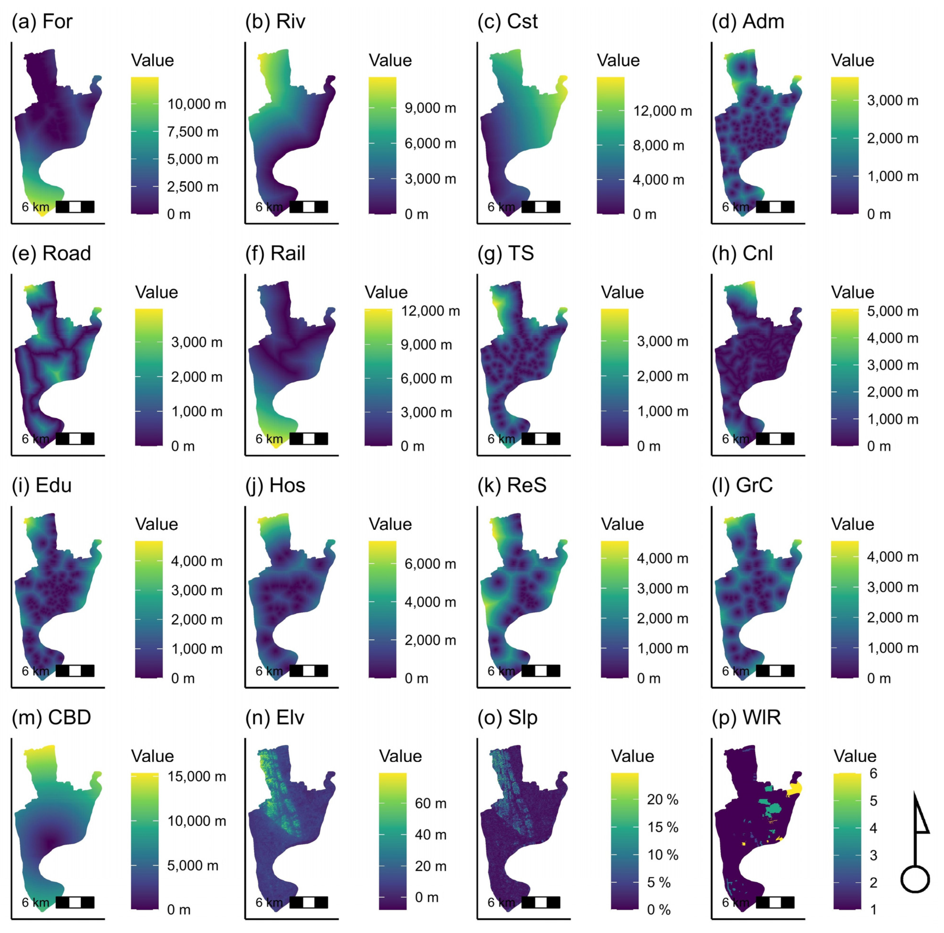
Forest (For), Major Roads (Rd), Railways (Rl), Major Canals (Cnl), Administrative Buildings (Adm), Growth Centers (GrC), Sea Coast (Cst), Rivers (Riv), Transportation Stations (TS), Educational Institutions (Edu), Hospitals (Hos), Recreation Sites (ReS), Central Business District (CBD)Prepared by the authors from the Google Earth Pro (GIS layers from Worldview)2022-
Waterlogging Risk (WlR)[44]2019-
Table 2. The influence of spatial factors contributed to the SDUS.
GeodetectorGlobal GWRFLocal GWRFDRF
RankVariableq StatisticVariableImportanceVariableImportanceVariableImportance
1CBD0.22CBD1846.28For26.34CBD0.57
2Riv0.14For1522.42Riv22.83Cst0.35
3Adm0.13Riv1135.10Cst22.16Riv0.35
4Hos0.11Cst1021.35GrC21.86For0.34
5TS0.1Adm998.64CBD21.18Adm0.31
6Elv0.08Hos924.58Rd20.84RS0.30
7Slp0.08TS812.77Hos20.79Elv0.28
8Cst0.07Rl753.76RS20.68Hos0.23
9GrC0.07RS733.09Rl20.28Rd0.22
10Cnl0.06Elv730.83Adm20.25GrC0.21
Disclaimer/Publisher’s Note: The statements, opinions and data contained in all publications are solely those of the individual author(s) and contributor(s) and not of MDPI and/or the editor(s). MDPI and/or the editor(s) disclaim responsibility for any injury to people or property resulting from any ideas, methods, instructions or products referred to in the content.

