Abstract
Mediterranean saline wetlands are significant ecological habitats defined by seasonal water availability and various biological communities, forming a unique ecotone that combines traits of both freshwater and marine environments. Moreover, they are regarded as notable natural and economic resources. Since the sustainable management of protected wetlands necessitates a multidisciplinary approach, the purpose of this study is to provide a comprehensive picture of the hydrological, hydrochemical, and ecological dynamics of a man-made groundwater dependent ecosystem (GDE) by combining remote sensing, hydrochemical data, geostatistical tools, and ecological indicators. The study area, called “Le Soglitelle”, is located in the Campania plain (Italy), which is close to the Domitian shoreline, covering a surface of 100 ha. The Normalized Difference Water Index (NDWI), a remote sensing-derived index sensitive to surface water presence, from Sentinel-2 was used to detect changes in the percentage of the wetland inundated area over time. Water samples were collected in four campaigns, and hydrochemical indexes were used to investigate the major hydrochemical seasonal processes occurring in the area. Geostatistical tools, such as principal component analysis (PCA) and independent component analysis (ICA), were used to identify the main hydrochemical processes. Moreover, faunal monitoring using waders was employed as an ecological indicator. Seasonal variation in the inundation area ranged from nearly 0% in summer to over 50% in winter, consistent with the severe climatic oscillations indicated by SPEI values. PCA and ICA explained over 78% of the total hydrochemical variability, confirming that the area’s geochemistry is mainly characterized by the saltwater sourced from the artesian wells that feed the wetland. The concentration of the major ions is regulated by two contrasting processes: evapoconcentration in summer and dilution and water mixing (between canals and ponds water) in winter. Cl−/Br− molar ratio results corroborated this double seasonal trend. The base exchange index highlighted a salinization pathway for the wetland. Bird monitoring exhibited consistency with hydrochemical monitoring, as the seasonal distribution clearly reflects the dual behaviour of this area, which in turn augmented the biodiversity in this GDE. The integration of remote sensing data, multivariate geostatistical analysis, geochemical tools, and faunal indicators represents a novel interdisciplinary framework for assessing GDE seasonal dynamics, offering practical insights for wetland monitoring and management.
1. Introduction
Mediterranean saline and transitional wetlands have been essential resources for human civilizations throughout history [1]. They represent unique ecosystems characterized by seasonal water availability and diverse biological communities [2]. These environments provide various valuable services such as regulation on local climate, water flow, nutrient cycling, air purification, wastewater treatment, soil erosion prevention, and flood control [3,4,5,6]. In addition, saline and transitional wetlands are part of a specific ecotone including freshwater and saltwater ecosystem characteristics. They are considered important natural resources due to their ecological and economical value [7]. Indeed, they are also known as biodiversity hotspots because of their large gradients of abiotic and biotic factors attracting a wide range of migratory birds and other endemic species [8]. This creates a complex system whose balance must be preserved to ensure its attractiveness to the species it houses [9]. This complexity is even exacerbated in drained wetlands which are composed of ponds and canals, where waters with different chemical compositions converge [10].
In light of this, the sustainable use and management of drained wetlands require careful planning and a deep scientific understanding of how these ecosystems work [11]. In this pursuit, in 1971 the Ramsar Convention on Wetlands was established with the aim to preserve these unique ecosystems [12]. Actually, the Ramsar Convention Strategic Plan’s targets have become key milestones of the Sustainable Development Goals (SDGs), underling the importance of wetland conservation [13].
To fulfil these aims, remote sensing (RS) can be used to dynamically monitor these types of ecosystems on both spatial and temporal scales in a real-time and simplified way [14]. For instance, the Normalized Difference Water Index (NDWI) obtained by RS data is extremely sensitive in detecting wetland hydrologic conditions and water coverage over time [15].
Moreover, in saline and transitional wetlands, it is crucial to understand both the salinity and hydrological dynamics as keys to future management plans [16], especially considering that these ecosystems are vulnerable to climate changes [17]. Contextually, halogens such as chloride (Cl−) and bromide (Br−) are frequently employed to fingerprint sources of salinity in groundwater and surface water because of their highly conservative transport properties [18]. Hence, the Cl−/Br− molar ratio is a reliable approach for identifying the salinity source of water samples [19]. These tracers have been widely applied to track wetland water dynamics [20], like mixing from different sources [21,22]. The base exchange (BEX) index is another valid tool widely used to determine water salinization/freshening pathways [23].
Moreover, the use of multivariate analysis, such as principal component analysis (PCA) and independent component analysis (ICA), allows us to simplify complex systems and obtain major readability of its main processes [24,25].
On the other hand, biological indicators are crucial factors for gaining important information about the seasonal environmental variations in a wetland [26]. Birds are broadly recognized as sensitive biological indicators of environmental conditions, including the seasonality of salinity and water availability in wetlands [27]. Their presence and abundance reflect the hydrological and chemical dynamics of these ecosystems, since many species show distinct ecological preferences for certain salinity level and water availability [28]. For instance, wader birds respond quickly to seasonal variations, moving according to the availability of suitable habitats [29]. Therefore, monitoring bird communities allows for the detection of the health and ecological functionality of wetlands [30].
Considering that the sustainable management of protected wetlands requires a multidisciplinary approach, this study aims to (i) identify the key seasonal hydrochemical processes, (ii) elucidate the primary drivers of salinity variation, and (iii) assess the ecological implications of these dynamics through avifaunal indicators. By integrating remote sensing, geochemical tools, and wader bird’s community data, a comprehensive set of insights was provided in order to support effective and adaptive management strategies for saline GDEs.
2. Study Area
The wetland area of this study, called “Le Soglitelle” (40°96′45.19″N; 14°01′78.97″E), is located in the Campania plain (CP), which is close to the Domitian shoreline, covering an area of 100 ha (Figure 1). The CP was formed in the Early Pleistocene by post orogenic extensional processes linked to strike-slip tectonics along the eastern Tyrrhenian boundary [31]. During the Late Pleistocene, the entire CP was exposed to subaerial conditions due to widespread volcanic activity, decreased tectonic subsidence rates, and eustatic regression [32], whereas during the Early Holocene the CP experienced a transgressive phase that led to the maximum shallow marine bay extension [33].
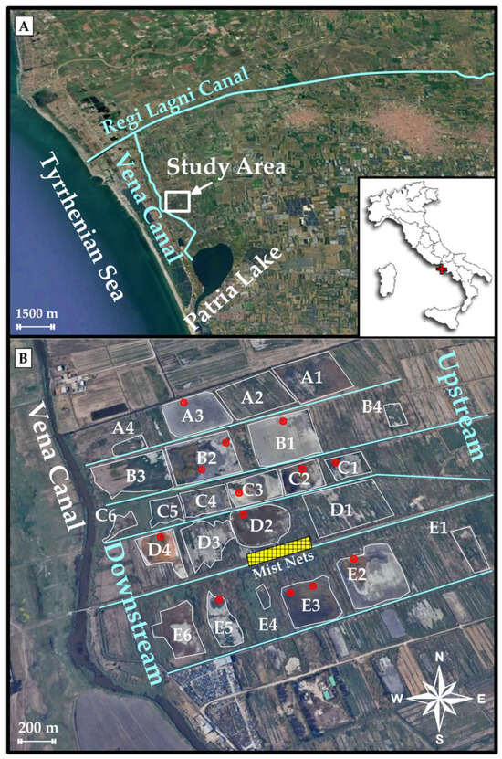
Figure 1.
(A) Sentinel-2 true colour mosaic image of the study area showing the boundaries of the “Le Soglitelle” area, the Regi Lagni Canal, the Vena Canal, and the Patria Lake; (B) Google Earth image of the “Le Soglitelle” showing the ponds (white lines) and channels (light blue lines), the wells’ location (red circles), and the mist nets’ location (yellow rectangular grid).
The studied wetland is roughly 2 km inland from the Tyrrhenian Sea and ranges in elevation from approximately −1 to 1 m above sea level. It is part of the regional natural reserve “Volturno Licola Falciano” and is bordered to the west by the urban area of “Castel Volturno” and on the other sides by agricultural areas and small industrial settlements. This area is a reclaimed land formed as a result of the drainage of the ancient Patria Lake. Its stratigraphy is characterized by layers of evaporitic muds dated around 3.2 ky BP [32]. The area is made up of a series of man-made ponds fed by artesian wells (approximately 35 m deep) that were built for illegal hunting purposes in the 1970s [34]. Ponds are interconnected by ditches that in turn are linked to canals discharging in the Vena (Figure 1).
The study area can be classified as a man-made GDE that refers to a wetland sustained by direct groundwater input, in this case through artificial artesian wells, making groundwater the primary hydrological driver. It is important to note that not all saline wetlands qualify as GDEs; indeed some coastal salt marshes can be influenced predominantly by tidal action and surface runoff and are not strictly dependent on groundwater [35].
The Soglitelle area is characterized by a typical Mediterranean climate, with hot summers and temperate rainy winters, with an average annual rainfall of 993 mm and a mean annual temperature around 17.0 °C from 1940 until 2000 with an increasing trend up to 18.9 °C in 2024 [36].
The vegetation is typical of brackish wetlands, with extensive salt marshes within the ponds and along their edges, while reeds and rushes are found along the canals. Furthermore, various bird species, including ones specifically protected by national and international guidelines, use this area to rest or breed [34,37].
3. Materials and Methods
3.1. Water Sample Collection and Analysis
Water samples from wells, ponds, and upstream and downstream of the canals were collected using PVC bailers (38 × 900 mm with a volume of 1000 mL) in four different sampling campaigns: March 2023, May 2023, July 2023, and December 2023 (Figures S1–S4 in Supplementary Information). The four sampling campaigns were strategically distributed across different seasons (spring, early summer, peak summer, and winter) to capture the seasonal variability of hydrochemical conditions, which is critical for understanding the dynamic behaviour of the study area. Samples of seawater, rain, the Regi Lagni Canal, and the Vena Canal were also collected and used as end-members. Rain samples were collected using a bulk dry and wet deposimeter sampler (Nesa srl, Vidor, Treviso, Italy). Electrical conductivity (EC), pH, oxidation reduction potential (ORP), and dissolved oxygen (DO) were measured on site using a HANNA Instruments multiparametric probe (HI98194) Woonsocket, RI, USA. The probe was calibrated before each sampling campaign and washed using Milli-Q water after each measurement. Samples were stored in HDPE bottles at 4 °C until analysis. Anion and cation analyses were carried out with an ICS-1000 Dionex-Thermo Scientific chromatography system equipped with an isocratic dual pump with an IonPac AS14A 4 × 250 mm column, the pre-column AG14A 4 × 50 mm, and an ASRS-Ultra 4 mm self-suppressor for anions and an IonPac CS12A 4 × 250 mm column, the pre-column CS12A 4 × 50 mm, and a CRS-500 4 mm self-suppressor for cations. The AS-40 Dionex auto-sampler was employed to run the analysis, while quality control (QC) samples were run every 20 samples. Dissolved organic carbon (DOC) was measured using a Pharmacia Biotech Ultrospec 2000 UV/VIS spectrophotometer following Cook et al.’s method [38]. Total alkalinity (TA) was quantified via titration, while dissolved inorganic carbon (DIC) was calculated with the PHREEQC-3 software [39], along with the saturation indexes (SIs) of gypsum, halite, calcite, and dolomite.
3.2. Sentinel-2 and Meteorological Data Collection
GMES Sentinel-2 is a European Space Agency (ESA) mission designed to systematically provide high resolution multispectral images of the global terrestrial surface [40]. Imagery and data were freely downloaded from the “Copernicus Browser”. Sentinel-2 L2A NDWI weekly data were extracted for each pond from 2016 to 2023. Only the images and the data with a cloud coverage <10% were selected. The NDWI dataset has a spatial resolution of 10 m, which is suitable for capturing fine-scale changes in water surface extent within small wetlands. NDWI was used to detected changes in the ponds’ water content. If NDWI >0 a water surface is detected, otherwise if NDWI < 0 a drought condition is detected. Sentinel-2 NDWI is calculated as follow [41]:
Daily mean, minimum, and maximum temperature and precipitation data from 2016 to 2023 were extracted by “Centro Funzionale Multirischi della Protezione Civile Regione Campania” [42]. Potential evapotranspiration (PET) data were downloaded by “Moderate Resolution Imaging Spectroradiometer (MODIS) instrument” of the National Aeronautics and Space Administration (NASA) [43].
3.3. Hydrological and Hydrochemical Data Elaboration
NDWI data were used to calculate the monthly water coverage percentage of the wetland using the following equation:
The standardized precipitation evapotranspiration index (SPEI) was assessed according to Begueria et al. [44]. Monthly water surplus/deficit was calculated as follow:
where P represents the monthly cumulative rainfall and PET is the monthly cumulative potential evapotranspiration. PET was chosen for this study because it is better suited to the wetlands’ abundant water conditions [45]. Since the SPEI is a climate-based drought index that relies exclusively on the difference between precipitation and potential evapotranspiration, hydrological fluxes such as river discharge or seawater intrusion were not considered, as they fall outside the conceptual framework of the index. To model the statistical distribution of the water balance, the data were fitted to a log-logistic distribution. This was later estimated using the genlogistic.fit() function of the SciPy library, which calculates the parameters of the distribution best suited for the observed data using the following function:
where α, β, and γ are the scale, shape, and position parameters, respectively. Then, the cumulative probability function was carried out for each observed water balance (B) value:
where X is the random variable representing the monthly water balance. P was transformed into a z-score of the standard normal distribution using the inverse quantile function:
where Φ−1 is the inverse quantile function of the normal standard distribution. For SPEI calculation the function np.precentile() of the NumPy library was utilized with a Monte Carlo simulation of 100,000 normally distributed random numbers. The SPEI categories are shown in Table 1.

Table 1.
SPEI categories.
The base exchange (BEX) index is a useful tool for understanding salinization/freshening dynamics. BEX was computed using the two following equations for the Ca- and Mg-rich aquifers, respectively [46]:
where 1.0716 and 0.8768 represent [Na + K + Mg]/Cl and [Na + K]/Cl for average seawater (meq/L), respectively. BEXCa could not be used in a dolomitic aquifer system because a considerable proportion of Mg comes from dolomite dissolution. For this reason, BEXMg was also used since dolomite minerals were present in the study area in significant quantities. BEX values can be positive, negative, or equal to zero. A positive BEX value suggests a freshening trend; a negative BEX value implies a salinization trend, while zero indicates stable conditions. PCA and ICA were employed to determine the main hydrogeochemical processes within the wetland. PCA was computed using the software IBM SPSS Statistics 20. The adequacy of the sample for PCA was assessed using the Kaiser–Meyer–Olkin (KMO) measure and Bartlett’s test of sphericity. The Varimax rotation through the Kaiser normalization procedure was selected, whereas variables exhibiting a rotated loading higher than ±0.60 were considered significant. ICA was performed to extract independent base vectors to determine the independent processes governing the geochemistry of the area [47]. It was assessed using the FastICA algorithm of the scikit-learn library, setting the number of independent components equal to the number of principal components found in PCA [48]. Saturation indexes (SIs) of gypsum, halite, calcite, and dolomite were calculated using the PHREEQC-3 software [39].
3.4. Wader Bird Catching and Ringing
Considering that waders are extremely susceptible to salinity and water content dynamics in a wetland, they were used as biological indicators for this study. Capture sessions were carried out on a decadal basis from 2019 to 2024. The COVID-19 emergency affected the execution of the monitoring activities throughout the year 2020 and, specifically, during the most critical months of the emergency. The dates of the ringing sessions were also chosen considering the local weather conditions, selecting days with little or no rain and wind. The trapping method employed consists of a 180 m long net with a surface area of 432 m2. The installation was divided into three transects of 108 m, 36 m, and 36 m positioned along the edge of the reed vegetation (Figure 1B). The mist nets utilized were 2.40 m tall and 12 m long, featuring four pockets and a 16 mm mesh. The nets were checked hourly. Following removal from the nets, the trapped individuals were placed in breathable canvas bags and transported to the field laboratory, where they were quickly analyzed, ringed, and released. For each bird, age, sex, and biometric measurements for the determination of the species were taken.
3.5. Wader Birds’ Data Elaboration
The number of bird species (NRSPEC) was obtained by aggregating the single individual’s data. In addition, bird species diversity (BSD) was calculated monthly via the Shannon–Weaver formula:
where s is the number of species and Pi is the proportion of individuals of species i to the total number of individuals observed in a month.
4. Results
4.1. Temporal Patterns of Drought and Water Availability
Figure 2 demonstrates the intermonth variability of the SPEI value and its related percentage of the inundated area of the wetland. The SPEI trend shows the typical shape of a Mediterranean area [49], characterized by summer SPEI values (Figure 2A) typical of severely dry conditions [50] and winter SPEI values between 1 and 2 corresponding to moderately and very wet periods, respectively. Starting from 2021 an increase in drought magnitude was registered, with SPEI values almost reaching −3. Indeed, the high temperature in summer leads to very intense water evaporation from the ponds, causing water scarcity in the wetland and even reaching water coverage percentages close to zero (Figure 2B). The intra-annual percentage of inundated area variation is the direct evidence of the two opposing climatic conditions described by the SPEI. Moreover, the marked contrast in pond-specific water coverage between the winter and summer seasons provides additional evidence of the spatial heterogeneity in water distribution, which is closely driven by seasonal climatic variability (Figure 2C). Considering the wetland hydroperiod, it falls in the fifth subsystem of the world wetland classification proposed by Junk [51], which includes wetlands along coastal rivers with small dimensions and temporary shallow waterbodies. As will be further discussed in the following paragraphs, this marked climatic variability significantly influences the hydrochemical processes that predominate in each season.
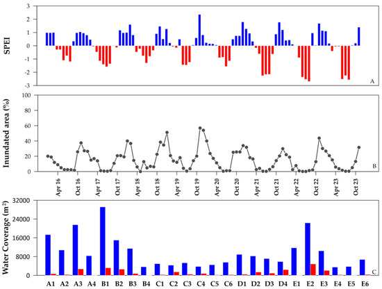
Figure 2.
(A) Monthly SPEI values from April 2016 to October 2023, where red bars represent negative values corresponding to dry periods, while blue bars represent positive values corresponding to wet periods. (B) Percentage of the wetlands’ inundated area with respect to the total wetland area. (C) Average water coverage (m2) for each pond during the winter (blue bars) and summer seasons (red bars).
4.2. Wetland Main Processes Based on PCA and ICA
PCA is widely used to investigate the distribution of chemical species and the main geochemical processes of an area [52,53]. To distinguish the processes occurring during the two different periods of the year, in this study two PCAs were performed: (i) one for the dry period sampling dataset and (ii) one for the wet period sampling dataset. Both were suitable for PCA, as indicated by KMO test values of 0.790 and 0.656, respectively, and Bartlett’s test of sphericity values of 1465.7 and 698.56, respectively, with a p value <0.005 for both datasets. PCA results are reported in Table 2, where significant loadings (≥±0.6) have been highlighted. According to the Kaiser criterion, four components were extracted for the dry dataset and five for the wet dataset, with a total explained variance of 81.9% and 78.5%, respectively. For the dry dataset, PC1 shows a strong correlation among seawater ions (Cl−, Br−, SO42−, K+, and Mg2+) and accounts for 45.7% of the total variance. This confirms that the geochemistry of the area is mainly influenced by the saltwater sourced from the artesian wells, further exacerbated by strong summer evaporation. PC2, which exhibits significant high loadings for NO3− and PO4− and explains 13.2% of the total variance, is related to the agricultural and farming leaching occurring upstream of the “Le Soglitelle” area and sourced by the input canals. PC3, with significant positive loadings for DO and DIC, explains 11.7% of the total variance. This result can be attributed to the area’s bioproductivity since oxygen and DIC cycles are linked to underwater biological processes [54,55]. Indeed, as observed by Cai et al. [56], CO2 inputs from SOM decomposition significantly influence the water DIC concentration in saltwater. PC4, which accounts for 11.3% of the cumulative variance, is related to redox processes along the gradient between the reducing conditions of the wells and the oxidizing conditions of ponds and canals. The PCA of the wet period mimics the one of the dry period, except for the behaviour of the seawater ions, which are distributed across PC1 and PC2, jointly explaining 45.2% of the cumulative variance. This confirms that the water sourced from the wells is the principal contributor to the geochemistry of the area even during the winter period. Despite this, PC1 exhibits significant positive loadings for TDS, Cl−, and Br−, while PC2 shows significant positive loadings for DOC, K+, Mg2+, and SO42−. This can be explained by the weaker evaporative processes in winter, meaning that only the concentration of the anions closely associated with evaporation is regulated by evapoconcentration/dilution processes. In contrast, although strong evapoconcentration was the main controlling factor for ions in solution during summer, in winter the ions related to PC2 are influenced by other processes likely linked to the biological activity of the various organisms. This trend is further supported by the results of the ICA (Table 3), which is used to identify independent processes that are unrelated to one another [57]. The mixing matrix of the dry period’s ICA reveals that Na+, K+, Ca2+, Cl−, Br−, and SO42− are all associated with a single independent component (IC), confirming that summer evaporation is the main factor regulating the concentration of these ions. In contrast, the mixing matrix of the wet period’s ICA shows that Cl− and Br− belong to a different IC compared to the other ions, highlighting the presence of two independent regulating processes.
Table 2.
Principal component loadings (varimax-rotated) for the different variables and their explained variance for the dry period and wet period datasets. Bold values are ≥0.60.
Table 3.
Independent component analysis mixing matrix for the different variables for the dry period and wet period datasets. Bold values are ≥0.50.
4.3. Sources and Drivers of Salinity Variability
Despite recent studies demonstrating that most of the salinity in this area originates from paleo-seawater affected by evapoconcentration processes [21,58], a Cl−/Br− vs. Cl− plot (Figure 3) was performed to gain deeper insights into the salinity drivers and variability in the samples collected during the four campaigns. The results of this analysis are consistent with those obtained from PCA and ICA. Indeed, depending on the season, two main processes are regulating the salinity in the area; most of the samples collected during the wet period are aligned along the mixing line between saltwater and freshwater end-members. In summer, on the other hand, intense pond water evaporation leads to the most saline samples, which were collected during the dry period and fell within the “seawater brines” box. Upstream canal samples, resulting from agricultural/farming leaching of the surrounding agricultural area [23], fall close to the “fertilizers” box. In contrast, downstream canals’ and some ponds’ samples are the result of the mixing processes occurring between the pond and upstream canal water.
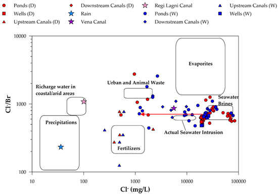
Figure 3.
Cl−/Br− molar ratio vs. Cl− plot. The red arrow indicates the mixing line among saltwater and freshwater end-members, while rectangular boxes are reported from Alcalà and Custodio [18]. Circles refer to pond samples; squares refer to well samples; triangles refer to upstream canal samples, and rhombuses refer to downstream canals. Red symbols and (D) refer to dry period data, while blue symbols and (W) refer to wet period data. The stars refer to the rain (light blue), Vena Canal (Violet), and Regi Lagni (Pink) end-members.
4.4. Initial Stages of Brine Formation
As discussed in the previous paragraph, most of the dry period pond samples fall in the “Seawater Brines” box. To further explore this, the evolution of major ions and minerals of the pond’s samples was also investigated. Cl− was used as an indicator of evaporation, and the behaviour of major ions and TDS was analyzed during Cl− fluctuations (Figure 4). High Cl− levels suggest an intense evapoconcentration process, as Cl− is only removed during the final stages of brine formation when halite precipitate [59]. The concentration of the major ions indicates that most of the dry period samples fell within stage 1.0 of brine development, corresponding to the onset of gypsum brines [60]. SI values provide further insights into the early-stage brine formation (Figure 5). All samples, except for a few ones, showed oversaturation for calcite and dolomite, which is consistent with the hydrogeochemistry of this area [21,61]. Indeed, despite the enrichment in alkali ions due to the water–rock interaction with the reworked volcanic material, the area maintains the original chemical composition of the lateral recharge from the neighbouring carbonate reliefs, as witness by the TA values being much higher than expected [62,63].
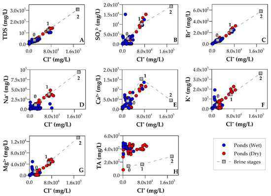
Figure 4.
(A–H) Scatter plots of major ions and TDS vs. Cl− (mg/L) used as an indicator of evaporation. Numbers represent the brine stage level. Grey squares represent the concentration values of the different ions for the corresponding brine stages reported by Fontes and Matray [60]. Blue circles refer to the ponds’ samples of the wet period, while red circles refer to the ponds’ samples of the dry period.
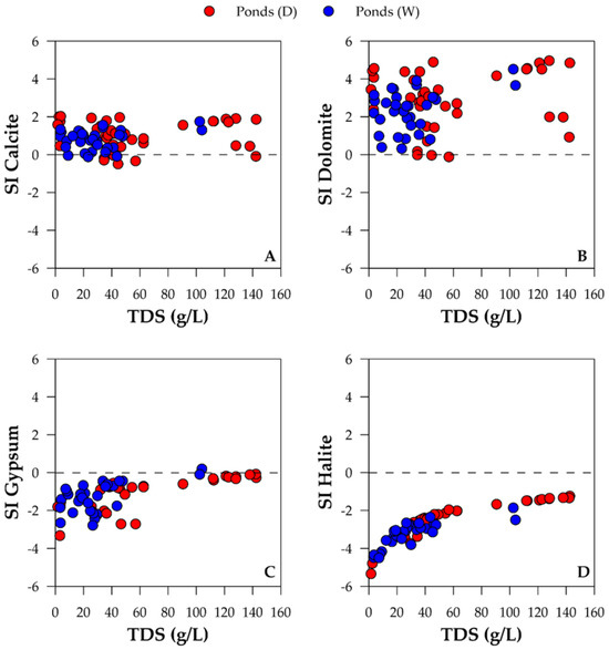
Figure 5.
Scatter plots: (A) calcite saturation index vs. TDS (g/L); (B) dolomite saturation index vs. TDS (g/L); (C) gypsum saturation index vs. TDS (g/L); (D) halite saturation index vs. TDS (g/L). Blue circles refer to the ponds’ samples during the wet period, while red circles refer to the ponds’ samples during the dry period.
4.5. Salinization Pathways
Since the aquifer consists of sediments from carbonate and dolomitic massifs surrounding the CP, Figure 6 depicts both the BEXCa and BEXMg indices. The BEX values of the well samples are negative since the salinity is attributable to evapoconcentrated paleo-seawater entrapped within the sediments [32] and subsequently flushed by recharge waters [21,58]. Therefore, a positive trend in BEX should be detected [64]. The values found in this study are most likely due to well intra-borehole mixing, where the upcoming of saltwater due to artesian conditions caused the salinization of the entire water column [65], resulting in negative BEX values for the wells’ samples. Likewise, as recently described by Habakaramo Macumu et al. [24], the slow release of salts from fragments of halophytes forming the peaty lenses, here consisting mainly of Salicornia europaea L., could represent an additional source of salinity contributing to a further decrease in the BEX values. However, additional investigations are needed to better understand the importance of this mechanism in this area. Pond samples predominantly show negative BEX due to the perennial input of saltwater from the wells, exacerbated by evaporative processes. Since the study area is located close to the Phlegraean Field volcanic area, Figure 6B provides further information on the role of carbonates and silicates in wetland hydrogeochemistry. The majority of the data fall below the bisectrix line, which may be attributed to the prevalence of bicarbonates in the aquifer matrix from which the wells draw water. Indeed, the average pH of the samples is around 7.8 since the dissolution of carbonates usually contributes to water alkalinity [66]. The few samples that exhibit clear silicate weathering are those collected during the dry period from the ponds. In this case, the Na+ excess over DIC could be imputable to the high salinity developed during summer evapoconcentration. Indeed, the SI of calcite was higher than 0.0, while the SI of halite was lower, meaning that the calcite precipitation, coupled with evapoconcentration, could have exacerbated the discrepancy between the concentration of Na+ and DIC in solution. Thus, the combination of DIC and Na+ can provide some constraints to identify the salinity sources, although it may be difficult to discern when volcanic deposits, calcareous deposits, and hypersaline environments coexist like in this area [67].
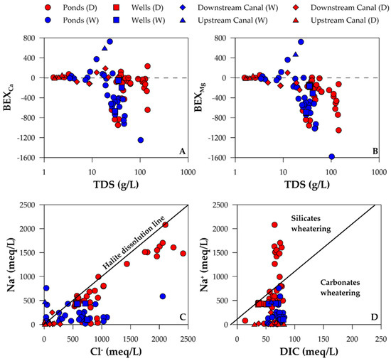
Figure 6.
Scatter Plots: (A) BEXCa vs. TDS; (B) BEXMg vs. TDS; (C) Na+ vs. Cl−; (D) Na+ vs. DIC. Blue circles refer to the ponds’ samples during the wet period, while red circles refer to the ponds’ samples during the dry period.
4.6. Wader Bird Monitoring
BSD and NRSPEC showed consistency with hydrochemical and climatic monitoring (Figure 7). The highest values of BSD and NRSPEC were found in the dry period when the brines were fully concentrated, and the water content of the area was significantly lower. Moreover, since 2022, a drop in August’s BSD and NRSPEC values has been detected compared to previous years.
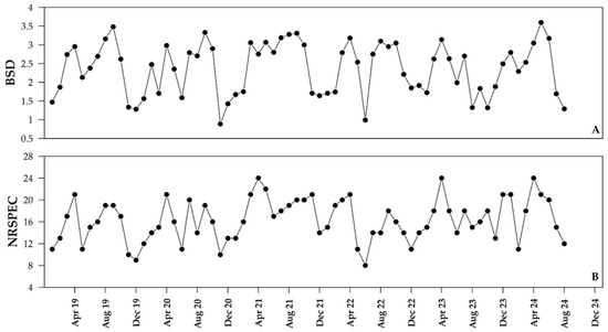
Figure 7.
(A) Monthly bird species diversity from April 2019 to August 2024 and (B) monthly number of bird species.
5. Discussion
The convergent approach of this study shows that dry periods are characterized by the evapoconcentration of the pond’s saltwater and the consequent salts’ precipitation, while wet periods are marked by the dilution of the pond’s water and the mixing processes between the different sources of water (rain, wells, and upstream canals). This high seasonal variability is a key factor for the unique biodiversity of the area, although the biological community consists mainly of organisms (both animals and plants) adapted to the area’ salinity. During the wet periods the biological community is characterized by species adapted to aquatic or semi-aquatic conditions, which exploit water availability and thermal stability. On the other hand, during the dry periods, the ecosystem is dominated by organisms highly specialized to survive in extremely severe salinity and drought conditions. As further evidence, the findings by Guglielmi et al. [68] showed, in this area, the highest richness in dragonfly (Odonata genus) species within the entire natural reserve, with “Volturno Licola Falciano” emerging as a hotspot for its conservation despite the trend that Odonata in Europe is declining [69]. Indeed, the dragonfly “double life” perfectly matches the double behaviour of the area because of the biphasic life cycle characterized by an aquatic larval stage and an adult winged life [70].
However, in winter, as confirmed by PCA, ICA, and the Cl−/Br− molar ratio, rainfall and upstream canal water dilute the saltwater sourced from the wells. In summer, on the other hand, intense pond water evaporation leads to the most saline samples having a typical seawater brine fingerprint. A further confirmation of this trend was given by the brine stages and SI analyses. Indeed, some of the pond samples collected during the dry period showed values close to gypsum saturation, while all ponds’ samples remained undersaturated for halite, confirming that the brines are still in the initial stage (1.0) of formation. This process represents a key factor in the ecological importance of this area since saltwater brines are characterized by extremely high primary productivity [71]. Moreover, gypsum precipitation in brines provides an ideal habitat for aquatic invertebrate communities [72] that represent a source of food for many aquatic birds [73].
Furthermore, the salinization pathway highlighted by the BEX index is alarming as it could be even boosted, especially considering that a decrease in precipitation (a 20% decrease by 2100) and an increase in temperature (between a 1.0 and 3.1 °C increase by 2100) are expected in the Mediterranean area [74].
Contextually, wader birds’ seasonal distribution is a clear indication of the dual behaviour of the area since summer evaporation leads to the formation of super-salty, muddy paddles, which are preferred environments for these birds to catch food. This is an important outcome considering that migratory species are globally becoming increasingly vulnerable to climate change and the resulting habitat losses to a disproportionate extent compared to non-migratory species [75]. The drop in BSD and NRSPEC in the last two years of monitoring could be related to the increased magnitude of the dry period, as demonstrated by the SPEI values, which led to the complete drying out of the ponds. This trend, coupled with a marked salinization pathway, may pose a serious risk to the conservation of this unique habitat and its hosts. Indeed, despite brines being highly productive environments, their progressive salinization could decrease their productivity and the overall ecological performance. For example, as stated by Saccò et al. [76], the number of aquatic invertebrate taxa decreases dramatically when TDS values exceeded 130 g/L, thus reducing the amount of food available for waders. Indeed, almost 70% of the species detected in this area suffer from global population declines, and some of them are classified as “Vulnerable” and “Near Threatened” by the International Union for Conservation of Nature (IUCN). Moreover, degradation is expected for 73% of Mediterranean wetlands [77], so hypersaline ecosystems are in dire need of tempestive conservation actions. Regulating and improving the inflow from freshwater end-members could limit, control, and even reverse the salinization trend [78]. Nevertheless, a considerable reduction in salinity patterns caused by freshwater restoration did not necessarily indicate simultaneous improvements in other wetland properties, and ecosystem restoration is known to be a long-term process [79].
Overall, while the individual components of this study approach are well established in the literature, the novelty of this study lies in the convergent approach used to analyze such a complex GDE. For instance, a combined strategy using RS data and field monitoring of soil and groundwater was successfully adopted by Alessandrino et al. [80] for investigating the plant salinity stress of a Mediterranean pine forest in a coastal back-barrier environment. By combining RS data, hydrochemical monitoring, multivariate statistical analyses, geochemical tools, and ecological indicators, this study offers a comprehensive approach to characterize seasonal ecohydrological dynamics. This convergence allows for a nuanced understanding of how climatic variability and groundwater input and chemistry jointly shape the behaviour of this system. Despite the known limitations of NDWI [81], such as the misclassification of turbid water, the results obtained in this study showed strong consistency with field observations. Although NDWI may not be suitable for precise hydrological budgeting due to its sensitivity to environmental noise, it remains an effective RS index for capturing seasonal fluctuations in wetland water availability, which is closely linked to hydrochemical and ecological dynamics.
6. Conclusions
This study shows how the integration of hydrochemical, RS, geostatistical, and ecological approaches is an effective method for understanding the environmental dynamics of an artificial saline GDE. NDWI monitoring confirmed the strong seasonal variability of the wetland inundated area, which is closely correlated to the SPEI, suggesting a high vulnerability of these ecosystems to ongoing and future climate change. The analysis of hydrochemical data allowed for the identification of the salinization/dilution dynamics, with evaporation playing a dominant role in dry periods and dilution in wetter ones. The application of multivariate techniques (PCA and ICA) revealed the main drivers of the hydrochemical processes and provided valuable insights for the management of the area. In parallel, the monitoring of the wading bird community has highlighted their role as bioindicators, showing a clear correlation between specific diversity, hydrochemical, and hydrological variations. Indeed, the increased severity of drought in recent years, coupled with the detected salinization pathway, poses a threat to the biodiversity of the area, with possible repercussions on this wetland to host migratory species in future. The results of this study emphasize the importance of a convergent approach to manage protected wetlands, providing quantitative tools to monitor and mitigate the effects of salinization and habitat loss. For example, regulating freshwater inputs to control the salinization trend, coupled with the continuous monitoring of hydrochemical and ecological conditions throughout the year, emerges as a priority action to ensure the hydroecological functionality of the wetland and its resilience to future climate change. Finally, it should be stressed that both hydrochemical, RS, and migratory bird monitoring could be easily replicated in other Mediterranean wetlands facing similar issues. In fact, it is precisely the choice of migratory and non-stationary species that allows them to be tracked and monitored in other comparable environments.
Supplementary Materials
The following supporting information can be downloaded at https://www.mdpi.com/article/10.3390/rs17122019/s1. Figure S1. Google Earth image of the “Le Soglitelle” showing the ponds (white lines) and channels (light blue lines), the wells’ location (red circles) and the observation points (yellow crosses) of the March 2023 sampling campaign. Figure S2. Google Earth image of the “Le Soglitelle” showing the ponds (white lines) and channels (light blue lines), the wells’ location (red circles) and the observation points (yellow crosses) of the May 2023 sampling campaign. Figure S3. Google Earth image of the “Le Soglitelle” showing the ponds (white lines) and channels (light blue lines), the wells’ location (red circles) and the observation points (yellow crosses) of the July 2023 sampling campaign. Figure S4. Google Earth image of the “Le Soglitelle” showing the ponds (white lines) and channels (light blue lines), the wells’ location (red circles) and the observation points (yellow crosses) of the December 2023 sampling campaign.
Author Contributions
Conceptualization, L.A., N.C. and M.M.; methodology, L.A. and N.C.; software, L.A.; validation, M.M., A.U. and N.C.; formal analysis, L.A.; investigation, L.A. and N.C.; resources, M.M.; data curation, L.A. and N.C.; writing—original draft preparation, L.A.; writing—review and editing, N.C., A.U. and M.M.; visualization, L.A.; supervision, M.M.; project administration, M.M.; funding acquisition, M.M. All authors have read and agreed to the published version of the manuscript.
Funding
This research was funded by the European Commission and MUR in the frame of the collaborative international consortium DATASET financed under the 2022 Joint call of the European Partnership 101060874—Water4All.
Data Availability Statement
Raw data are available in Supplementary Material S1. Other elaborated data will be made available by the authors upon request.
Acknowledgments
The authors would like to thank the European Commission and MUR for funding the framework of the collaborative international consortium DATASET (Groundwater salinization and pollution assessment tool: a holistic approach for coastal areas, Water4All_00084), financed under the 2022 Joint call of the European Partnership 101060874—Water4All.
Conflicts of Interest
The authors declare no conflicts of interest.
Abbreviations
The following abbreviations are used in this manuscript:
| GDE | Groundwater dependent ecosystem |
| NDWI | Normalized Difference Water Index |
| PCA | Principal Component Analysis |
| ICA | Independent Component Analysis |
| IC | Independent Component |
| RS | Remote Sensing |
| CP | Campania Plain |
| EC | Electrical Conductivity |
| ORP | Oxidation Reduction Potential |
| DO | Dissolved Oxygen |
| QC | Quality Control |
| DIC | Dissolved Inorganic Carbon |
| TA | Total Alkalinity |
| SI | Saturation Index |
| ESA | European Space Agency |
| PET | Potential Evapotranspiration |
| MODIS | Moderate Resolution Imaging Spectroradiometer |
| NASA | National Aeronautics and Space Administration |
| SPEI | Standardized Precipitation Evapotranspiration Index |
| BEX | Base Exchange |
| KMO | Kaiser–Meyer–Olkin |
| NRSPEC | Number of Birds Species |
| BSD | Bird Species Diversity |
| TDSs | Total Dissolved Solids |
| IUCN | International Union of Conservation of Nature |
References
- Paul, V.G.; Mormile, M.R. A case for the protection of saline and hypersaline environments: A microbiological perspective. Microb. Ecol. 2017, 93, 8. [Google Scholar] [CrossRef] [PubMed]
- Guo, M.; Li, J.; Sheng, C.; Xu, J.; Wu, L. A review of wetland remote sensing. Sensors 2017, 17, 777. [Google Scholar] [CrossRef] [PubMed]
- Liu, J.; Guo, Y.; Han, J.; Yang, F.; Shen, N.; Sun, F.; Wei, Y.; Yuan, P.; Wang, J. Nature-based solutions for landscape performance evaluation-Handan Garden Expo Park’s “Clear as a Drain” artificial wetland as an example. Land 2024, 13, 973. [Google Scholar] [CrossRef]
- Hambäck, P.A.; Dawson, L.; Geranmayeh, P.; Jarsjö, J.; Kačergytė, I.; Peacock, M.; Collentine, D.; Destouni, G.; Futter, M.; Hugelius, G.; et al. Trade-offs and synergies in wetland multifunctionality: A scaling issue. Sci. Total Environ. 2023, 862, 160746. [Google Scholar] [CrossRef]
- Hassan, I.; Chowdhury, S.R.; Prihartato, P.K.; Razzak, S.A. Wastewater treatment using constructed wetlands: Current trends and future potential. Processes 2021, 11, 1917. [Google Scholar] [CrossRef]
- Xu, X.; Chen, M.; Yang, G.; Jiang, B.; Zhang, J. Wetland ecosystem services research: A critical review. Glob. Ecol. Conserv. 2020, 22, e01027. [Google Scholar] [CrossRef]
- Pérez-Ruzafa, A.; Marcos, C.; Pérez-Ruzafa, I.M. Mediterranean coastal lagoons in an ecosystem and aquatic resources management context. Phys. Chem. Earth A/B/C 2011, 36, 160–166. [Google Scholar] [CrossRef]
- Perennou, C.; Gaget, E.; Galewski, T.; Geijzendorffer, I.; Guelmami, A. Evolution of wetlands in the Mediterranean region. In Water Resources in the Mediterranean Region; Elsevier: Amsterdam, The Netherlands, 2020; pp. 297–320. [Google Scholar]
- Sharma, L.K.; Naik, R. Wetland ecosystems. In Conservation of Saline Wetland Ecosystems; Springer Nature: Singapore, 2024; pp. 3–32. [Google Scholar]
- Kudray, G.M.; Gale, M.R. Evaluation of National Wetland Inventory Maps in a Heavily Forested Region in the Upper Great Lakes. Wetlands 2000, 20, 581–587. [Google Scholar] [CrossRef]
- Carol, E.; del Pilar Alvarez, M.; Arcia, M.; Candanedo, I. Surface and groundwater flow exchanges and lateral hydrological connectivity in environments of the Matusagaratí Wetland, Panama. Sci. Total Environ. 2024, 927, 172293. [Google Scholar] [CrossRef]
- Gardner, R.C.; Davidson, N.C. The Ramsar Convention. In Wetlands; Springer: Berlin/Heidelberg, Germany, 2011; pp. 189–203. [Google Scholar]
- Mohanty, S.; Pandey, P.C.; Pandey, M.; Srivastava, P.K.; Dwivedi, C.S. Wetlands contribution and linkage to support SDGs, its indicators and targets-A critical review. Sustain. Develop. 2024, 32, 5348–5392. [Google Scholar] [CrossRef]
- Jie, W.; Xiao, C.; Zhang, C.; Zhang, E.; Li, J.; Wang, B.; Niu, H.; Dong, S. Remote sensing-based dynamic monitoring and environmental change of wetlands in the southern Mongolian Plateau from 2010 to 2018. China Geol. 2021, 4, 1–13. [Google Scholar] [CrossRef]
- Talukdar, S.; Pal, S. Effects of damming on the hydrological regime of Punarbhaba River basin wetlands. Ecol. Eng. 2019, 135, 61–74. [Google Scholar] [CrossRef]
- Levy, Z.F.; Mills, C.T.; Lu, Z.; Goldhaber, M.B.; Rosenberry, D.O.; Mushet, D.M.; Lautz, L.K.; Zhou, X.; Siegel, D.I. Using halogens (Cl, Br, I) to understand the hydrogeochemical evolution of drought-derived saline porewater beneath a prairie wetland. Chem. Geol. 2018, 476, 191–207. [Google Scholar] [CrossRef]
- Scholz, M. Impact of climate change on wetland ecosystems. In Wetlands for Water Pollution Control; Elsevier: Amsterdam, The Netherlands, 2024; pp. 403–430. [Google Scholar]
- Alcalá, F.J.; Custodio, E. Using the Cl/Br ratio as a tracer to identify the origin of salinity in aquifers in Spain and Portugal. J. Hydrol. 2008, 359, 189–207. [Google Scholar] [CrossRef]
- Rao, U.; Hollocher, K.; Sherman, J.; Eisele, I.; Frunzi, M.N.; Swatkoski, S.J.; Hammons, A.L. The use of 36Cl and chloride/bromide ratios in discerning salinity sources and fluid mixing patterns: A case study at Saratoga Springs. Chem. Geol. 2005, 222, 94–111. [Google Scholar] [CrossRef]
- Bodin, H.; Mietto, A.; Ehde, P.M.; Persson, J.; Weisner, S.E.B. Tracer behaviour and analysis of hydraulics in experimental free water surface wetlands. Ecol. Eng. 2012, 49, 201–211. [Google Scholar] [CrossRef]
- Colombani, N.; Alessandrino, L.; Gaiolini, M.; Gervasio, M.P.; Ruberti, D.; Mastrocicco, M. Unravelling the salinity origins in the coastal aquifer/aquitard system of the Volturno River (Italy). Water Res. 2024, 263, 122145. [Google Scholar] [CrossRef]
- Alessandrino, L.; Gaiolini, M.; Cellone, F.A.; Colombani, N.; Mastrocicco, M.; Cosma, M.; Da Lio, C.; Donnici, S.; Tosi, L. Salinity origin in the coastal aquifer of the Southern Venice lowland. Sci. Total Environ. 2023, 905, 167058. [Google Scholar] [CrossRef]
- Mastrocicco, M.; Gervasio, M.P.; Busico, G.; Colombani, N. Natural and anthropogenic factors driving groundwater resources salinization for agricultural use in the Campania plains (Southern Italy). Sci. Total Environ. 2021, 758, 144033. [Google Scholar] [CrossRef]
- Habakaramo Macumu, P.; Gaiolini, M.; Ofori, A.; Mastrocicco, M.; Colombani, N. Additional sources of salinity and heavy metals from plant residues of peaty horizons in the Po River lowland (Italy). Sci. Total Environ. 2024, 957, 177671. [Google Scholar] [CrossRef]
- Xue, J.; Lee, C.; Wakeham, S.G.; Armstrong, R.A. Using principal components analysis (PCA) with cluster analysis to study the organic geochemistry of sinking particles in the ocean. Org. Geochem. 2011, 42, 356–367. [Google Scholar] [CrossRef]
- Bhaduri, D.; Sihi, D.; Bhowmik, A.; Verma, B.C.; Munda, S.; Dari, B. A review on effective soil health bio-indicators for ecosystem restoration and sustainability. Front. Microbiol. 2022, 13, 938481. [Google Scholar] [CrossRef] [PubMed]
- Mott, R.; Prowse, T.A.A.; Jackson, M.V.; Rogers, D.J.; O’Connor, J.A.; Brookes, J.D.; Cassey, P. Measuring habitat quality for waterbirds: A review. Ecol. Evol. 2023, 13, 4. [Google Scholar] [CrossRef] [PubMed]
- Aslan, H.; Elipek, B.; Gönülal, O.; Baytut, Ö.; Kurt, Y.; İnanmaz, Ö.E. Gökçeada Salt Lake: A Case Study of Seasonal Dynamics of Wetland Ecological Communities in the Context of Anthropogenic Pressure and Nature Conservation. Wetlands 2021, 41, 2. [Google Scholar] [CrossRef]
- Prateek, A.M.; Mishra, H.; Kumar, V.; Kumar, A. Temporal pattern in foraging behaviour of Vanellus malabaricus in relation to different seasons and habitats. Avian Biol. Res. 2024, 17, 22–30. [Google Scholar] [CrossRef]
- Qiu, J.; Zhang, Y.; Ma, J. Wetland habitats supporting waterbird diversity: Conservation perspective on biodiversity-ecosystem functioning relationship. J. Environ. Manag. 2024, 357, 120663. [Google Scholar] [CrossRef]
- Milia, A.; Torrente, M.M. Late-Quaternary volcanism and transtensional tectonics in the Bay of Naples, Campanian continental margin, Italy. Mineral. Petrol. 2003, 79, 49–65. [Google Scholar] [CrossRef]
- Sacchi, M.; Molisso, F.; Pacifico, A.; Vigliotti, M.; Sabbarese, C.; Ruberti, D. Late-Holocene to recent evolution of Lake Patria, South Italy: An example of a coastal lagoon within a Mediterranean delta system. Glob. Planet. Change 2014, 117, 9–27. [Google Scholar] [CrossRef]
- Amorosi, A.; Pacifico, A.; Rossi, V.; Ruberti, D. Late Quaternary incision and deposition in an active volcanic setting: The Volturno valley fill, southern Italy. Sediment. Geol. 2012, 282, 307–320. [Google Scholar] [CrossRef]
- Usai, A. L’Inanellamento Nella Zona Umida “Le Soglitelle” Report Anno 2020-“Le Soglitelle” Bird Ringing Report 2020; Technical Report; Istituto di Gestione della Fauna: Naples, Italy, 2021. [Google Scholar]
- Kløve, B.; Ala-aho, P.; Bertrand, G.; Boukalova, Z.; Ertürk, A.; Goldscheider, N.; Ilmonen, J.; Karakaya, N.; Kupfersberger, H.; Kvœrner, J.; et al. Groundwater dependent ecosystems. Part I: Hydroecological status and trends. Environ. Sci. Policy 2011, 14, 770–781. [Google Scholar] [CrossRef]
- Copernicus Browser. Available online: https://browser.dataspace.copernicus.eu/ (accessed on 1 April 2025).
- Mastronardi, D.; Esse, E.; Balestrieri, R.; De Rosa, D.; Giannotti, M.; Piciocchi, S. The bird communities of four wetlands on the Tyrrhenian coast NW of Naples in relation to human disturbance. Riv. Ital. Ornitol. 2012, 82, 1–2. [Google Scholar] [CrossRef][Green Version]
- Cook, S.; Peacock, M.; Evans, C.D.; Page, S.E.; Whelan, M.J.; Gauci, V.; Kho, L.K. Quantifying tropical peatland dissolved organic carbon (DOC) using UV-visible spectroscopy. Water Res. 2017, 115, 229–235. [Google Scholar] [CrossRef] [PubMed]
- Parkhurst, D.L.; Appelo, C.A.J. Description of Input and Examples for PHREEQC Version 3: A Computer Program for Speciation, Batch-reaction, One-dimensional Transport, and Inverse Geochemical Calculations (No. 6-A43). USGS 2013. US Geol. Surv. Tech. Methods 2013, 6, 487. [Google Scholar]
- European Space Agency (ESA). Sentinel-2: ESA’s Optical High-Resolution Mission for GMES Operational Services. ESA SP-1322/2. March 2012. Available online: https://www.esa.int/About_Us/ESA_Publications/ESA_SP-1322_2_Sentinel_2 (accessed on 1 April 2025).
- McFeeters, S.K. The use of the Normalized Difference Water Index (NDWI) in the delineation of open water features. Int. J. Remote Sens. 1996, 17, 1425–1432. [Google Scholar] [CrossRef]
- Centro Funzionale Multirischi Della Protezione Civile Regione Campania. Available online: https://centrofunzionale.regione.campania.it/ (accessed on 1 April 2025).
- Moderate Resolution Imaging Spectroradiometer (MODIS). Available online: https://www.spiedigitallibrary.org/conference-proceedings-of-spie/1939/0000/Moderate-Resolution-Imaging-Spectroradiomete-MODIS/10.1117/12.152835.short#_=_ (accessed on 1 April 2025).
- Beguería, S.; Vicente-Serrano, S.M.; Reig, F.; Latorre, B. Standardized precipitation evapotranspiration index (SPEI) revisited: Parameter fitting, evapotranspiration models, tools, datasets and drought monitoring. Int. J. Climatol. 2013, 34, 3001–3023. [Google Scholar] [CrossRef]
- Jin, X.; Qiang, H.; Zhao, L.; Jiang, S.; Cui, N.; Cao, Y.; Feng, Y. SPEI-based analysis of spatio-temporal variation characteristics for annual and seasonal drought in the Zoige Wetland, Southwest China from 1961 to 2016. Theor. Appl. Climatol. 2019, 139, 711–725. [Google Scholar] [CrossRef]
- Stuyfzand, P.J. Base exchange indices as indicators of salinization or freshening of (coastal) aquifers. In Proceedings of the 18th Salt Water Intrusion Meeting (SWIM), Cartagena, Spain, 31 May–3 June 2004. [Google Scholar]
- Iwamori, H.; Yoshida, K.; Nakamura, H.; Kuwatani, T.; Hamada, M.; Haraguchi, S.; Ueki, K. Classification of geochemical data based on multivariate statistical analyses: Complementary roles of cluster, principal component, and independent component analyses. Geochem. Geophys. 2017, 18, 994–1012. [Google Scholar] [CrossRef]
- Shahrestani, S.; Cohen, D.R.; Mokhtari, A.R. A comparison of PCA and ICA in geochemical pattern recognition of soil data: The case of Cyprus. J. Geochem. Explor. 2024, 264, 107539. [Google Scholar] [CrossRef]
- Perez, M.; Lombardi, D.; Bardino, G.; Vitale, M. Drought assessment through actual evapotranspiration in Mediterranean vegetation dynamics. Ecol Indic. 2024, 166, 112359. [Google Scholar] [CrossRef]
- Li, B.; Zhou, W.; Zhao, Y.; Ju, Q.; Yu, Z.; Liang, Z.; Acharya, K. Using the SPEI to assess recent climate change in the Yarlung Zangbo River Basin, South Tibet. Water 2015, 7, 5474–5486. [Google Scholar] [CrossRef]
- Junk, W.J. World wetlands classification: A new hierarchic hydro-ecological approach. Wetl. Ecol. Manag. 2024, 32, 975–1001. [Google Scholar] [CrossRef]
- Zhao, K.; Bao, K.; Yan, Y.; Neupane, B.; Gao, C. Spatial distribution of potentially harmful trace elements and ecological risk assessment in Zhanjiang mangrove wetland, South China. Mar. Pollut. Bull. 2022, 182, 114033. [Google Scholar] [CrossRef] [PubMed]
- Colombani, N.; Cuoco, E.; Mastrocicco, M. Origin and pattern of salinization in the Holocene aquifer of the southern Po Delta (NE Italy). J. Geochem. Explor. 2017, 175, 130–137. [Google Scholar] [CrossRef]
- Parker, S.R.; Darvis, M.N.; Poulson, S.R.; Gammons, C.H.; Stanford, J.A. Dissolved oxygen and dissolved inorganic carbon stable isotope composition and concentration fluxes across several shallow floodplain aquifers and in a diffusion experiment. Biogeochemistry 2013, 117, 539–552. [Google Scholar] [CrossRef]
- Gammons, C.H.; Babcock, J.N.; Parker, S.R.; Poulson, S.R. Diel cycling and stable isotopes of dissolved oxygen, dissolved inorganic carbon, and nitrogenous species in a stream receiving treated municipal sewage. Chem. Geol. 2010, 238, 44–55. [Google Scholar] [CrossRef]
- Cai, W.J.; Dai, M.; Wang, Y.; Zhai, W.; Huang, T.; Chen, S.; Zhang, F.; Chen, Z.; Wang, Z. The biogeochemistry of inorganic carbon and nutrients in the Pearl River estuary and the adjacent Northern South China Sea. Cont. Shelf Res. 2004, 24, 1301–1319. [Google Scholar] [CrossRef]
- Hyvärinen, A. Independent component analysis: Recent advances. Philos. Trans. R. Soc. 2013, 371, 20110534. [Google Scholar] [CrossRef]
- Schiavo, M.; Colombani, N.; Mastrocicco, M. Modeling stochastic saline groundwater occurrence in coastal aquifers. Water Res. 2023, 235, 119885. [Google Scholar] [CrossRef]
- Vahidipour, M.; Raeisi, E.; van der Zee, S.E.A.T.M. Temporal dynamics of inundation area, hydrochemistry and brine in Bakhtegan Lake, South-Central Iran. J. Hydrol. Reg. 2024, 52, 101714. [Google Scholar] [CrossRef]
- Fontes, J.C.; Matray, J.M. Geochemistry and origin of formation brines from the Paris Basin, France. Chem. Geol. 1993, 109, 149–175. [Google Scholar] [CrossRef]
- Corniello, A.; Ducci, D.; Stellato, L.; Stevenazzi, S.; Massaro, L.; Del Gaudio, E. Combining groundwater budget, hydrochemistry and environmental isotopes to identify the groundwater flow in carbonate aquifers located in Campania Region (Southern Italy). J. Hydrol. Reg. Stud. 2024, 53, 101790. [Google Scholar] [CrossRef]
- Bordbar, M.; Busico, G.; Sirna, M.; Tedesco, D.; Mastrocicco, M. A multi-step approach to evaluate the sustainable use of groundwater resources for human consumption and agriculture. J. Environ. Manag. 2023, 347, 119041. [Google Scholar] [CrossRef] [PubMed]
- Corniello, A.; Ducci, D. Hydrogeochemical characterization of the main aquifer of the “Litorale Domizio-Agro Aversano NIPS” (Campania—Southern Italy). J. Geochem. Explor. 2014, 137, 1–10. [Google Scholar] [CrossRef]
- Meyer, R.; Engesgaard, P.; Sonnenborg, T.O. Origin and dynamics of saltwater intrusion in a regional aquifer: Combining 3-D saltwater modeling with geophysical and geochemical data. Water Resour. Res. 2023, 55, 1792–1813. [Google Scholar] [CrossRef]
- Gattacceca, J.C.; Vallet-Coulomb, C.; Mayer, A.; Claude, C.; Radakovitch, O.; Conchetto, E.; Hamelin, B. Isotopic and geochemical characterization of salinization in the shallow aquifers of a reclaimed subsiding zone: The southern Venice Lagoon coastland. J. Hydrol. 2009, 378, 46–61. [Google Scholar] [CrossRef]
- Castrillon-Munoz, F.J.; Gibson, J.J.; Birks, S.J. Carbon dissolution effects on pH changes of RAMP lakes in northeastern Alberta, Canada. J. Hydrol. Reg. Stud. 2022, 40, 101045. [Google Scholar] [CrossRef]
- Ruberti, D.; Buffardi, C.; Sacchi, M.; Vigliotti, M. The late Pleistocene-Holocene changing morphology of the Volturno delta and coast (northern Campania, Italy): Geological architecture and human influence. Quat. Int. 2022, 625, 14–28. [Google Scholar] [CrossRef]
- Guglielmi, M.; De Filippo, G.; Elicio, F.; Usai, A. A review of knowledge on dragonflies and damselflies in the Regional Nature Reserve “Foce Volturno – Costa di Licola”. BORNH Bull. Reg. Nat. Hist. 2024, 4, 32–43. [Google Scholar]
- De Knijf, G.; Billqvist, M.; van Grunsven, R.; Allen, D.; Assandri, G.; Bellotto, V.; Bruslund, S.; Bedjanič, M.; Conze, K.J.; Díaz Martínez, C.; et al. European Dragonflies: Moving from Assessment to Conservation Planning. A Report to the European Commission by the IUCN SSC Dragonfly Specialist Group and the IUCN SSC Conservation Planning Specialist Group; Conservation Planning Specialist Group: Apple Valley, MN, USA, 2024. [Google Scholar]
- Oertli, B. The use of dragonflies in the assessment and monitoring of aquatic habitats. In Dragonflies and Damselflies: Model Organisms for Ecological and Evolutionary; Oxford University Press: Oxford, UK, 2008; pp. 79–96. [Google Scholar]
- Schagerl, M. Soda Lakes of East Africa; Springer International Publishing: Cham, Switzerland, 2016. [Google Scholar]
- Finlayson, C.M.; Milton, G.R.; Prentice, R.C.; Davidson, N.C. The Wetland Book; Springer: Dordrecht, The Netherlands, 2018. [Google Scholar]
- Gutiérrez, J.S. Living in Environments with Contrasting Salinities: A Review of Physiological and Behavioural Responses in Waterbirds. Ardeola 2014, 61, 233–256. [Google Scholar] [CrossRef]
- Seker, M.; Gumus, V. Projection of temperature and precipitation in the Mediterranean region through multi-model ensemble from CMIP6. Atmos. Res. 2022, 280, 106440. [Google Scholar] [CrossRef]
- Kirby, J.S.; Stattersfield, A.J.; Butchart, S.H.M.; Evans, M.I.; Grimmett, R.F.A.; Jones, V.R.; O’Sullivan, J.; Tucker, G.M.; Newton, I. Key conservation issues for migratory land- and waterbird species on the world’s major flyways. Bird Conserv. Int. 2008, 18, 49–73. [Google Scholar] [CrossRef]
- Saccò, M.; White, N.E.; Harrod, C.; Salazar, G.; Aguilar, P.; Cubillos, C.F.; Meredith, K.; Baxter, B.K.; Oren, A.; Anufriieva, E.; et al. Salt to conserve: A review on the ecology and preservation of hypersaline ecosystems. Biol. Rev. 2021, 96, 2828–2850. [Google Scholar] [CrossRef] [PubMed]
- Lefebvre, G.; Redmond, L.; Germain, C.; Palazzi, E.; Terzago, S.; Willm, L.; Poulin, B. Predicting the vulnerability of seasonally-flooded wetlands to climate change across the Mediterranean Basin. Sci. Total Environ. 2019, 692, 546–555. [Google Scholar] [CrossRef] [PubMed]
- Middleton, B.A.; Boudell, J. Salinification of Coastal Wetlands and Freshwater Management to Support Resilience. Ecosyst. Health Sustain. 2023, 9, 83. [Google Scholar] [CrossRef]
- Huang, L.; Zhang, G.; Bai, J.; Xia, Z.; Wang, W.; Jia, J.; Wang, X.; Liu, X.; Cui, B. Desalinization via freshwater restoration highly improved microbial diversity, co-occurrence patterns and functions in coastal wetland soils. Sci. Total Environ. 2021, 765, 142769. [Google Scholar] [CrossRef]
- Alessandrino, L.; Giuditta, E.; Faugno, S.; Colombani, N.; Mastrocicco, M. Direct and Remote Sensing Monitoring of Plant Salinity Stress in a Coastal Back-Barrier Environment: Mediterranean Pine Forest Stress and Mortality as a Case Study. Remote Sens. 2024, 16, 3150. [Google Scholar] [CrossRef]
- Albertini, C.; Gioia, A.; Iacobellis, V.; Manfreda, S. Detection of Surface Water and Floods with Multispectral Satellites. Remote Sens. 2022, 14, 6005. [Google Scholar] [CrossRef]
Disclaimer/Publisher’s Note: The statements, opinions and data contained in all publications are solely those of the individual author(s) and contributor(s) and not of MDPI and/or the editor(s). MDPI and/or the editor(s) disclaim responsibility for any injury to people or property resulting from any ideas, methods, instructions or products referred to in the content. |
© 2025 by the authors. Licensee MDPI, Basel, Switzerland. This article is an open access article distributed under the terms and conditions of the Creative Commons Attribution (CC BY) license (https://creativecommons.org/licenses/by/4.0/).