High-Fidelity 3D Gaussian Splatting for Exposure-Bracketing Space Target Reconstruction: OBB-Guided Regional Densification with Sobel Edge Regularization

Abstract

In this paper, a novel optimization framework based on 3D Gaussian splatting (3DGS) for high-fidelity 3D reconstruction of space targets under exposure bracketing conditions is studied. In the considered scenario, multi-view optical imagery captures space targets under complex and dynamic illumination, where severe inter-frame brightness variations degrade reconstruction quality by introducing photometric inconsistencies and blurring fine geometric details. Unlike existing methods, we explicitly address these challenges by integrating exposure-aware adaptive refinement and edge-preserving regularization into the 3DGS pipeline. Specifically, we propose an exposure bracketing-oriented bounding box (OBB) regional densification strategy to dynamically identify and refine under-reconstructed regions. In addition, we introduce a Sobel edge regularization mechanism to guide the learning of sharp geometric features and improve texture fidelity. To validate the framework, experiments are conducted on both a custom OBR-ST dataset and the public SHIRT dataset, demonstrating that our method significantly outperforms state-of-the-art techniques in geometric accuracy and visual quality under exposure-bracketing scenarios. The results highlight the effectiveness of our approach in enabling robust in-orbit perception for space applications.

1. Introduction

Three-dimensional (3D) reconstruction of space targets is critical for in-orbit perception, enabling geometric and texture recovery from multi-view imagery. This process plays a critical role in assessing and understanding the condition of space targets during operation. By analyzing multi-view observations, 3D reconstruction helps extract structural and surface information, which supports tasks such as status evaluation and fault diagnosis [1,2,3,4,5,6,7]. A notable example is Astroscale’s ELSA-d mission, which completed the first autonomous rendezvous with an uncontrolled space target in 2022. Although the mission was suspended due to thruster malfunctions, it highlighted the importance of 3D reconstruction for space debris removal technologies [8,9]. As 3D reconstruction becomes increasingly vital for on-orbit servicing (OOS), space situational awareness (SSA), and deep space exploration, it continues to attract significant attention [10].

During on-orbit close-range imaging, the relative motion between the chaser and the space target continuously changes the illumination direction; together with diverse surface-reflectance properties and the coexistence of direct sunlight and deep shadows, fixed-exposure settings seldom capture the full range of scene details. To enlarge the dynamic range, exposure bracketing [11,12] is widely adopted to rapidly capture low-, medium-, and high-exposure frames. However, the resulting drastic inter-frame brightness gaps fundamentally violate the photometric-consistency assumption on which most 3D reconstruction algorithms rely. Against this backdrop, the classic workflow for reconstructing space targets still unfolds in the following three stages: (i) extraction and matching of image features such as SIFT [13] and SURF [14] to build view correspondences; (ii) recovery of the chaser’s camera trajectory and a sparse point cloud via Structure from Motion (SfM) [15,16,17]; and (iii) densification to a detailed point cloud or mesh with multi-view stereo (MVS) [18]. Because this pipeline hinges on reliable cross-view feature matches, the severe exposure differences introduced by bracketing often degrade SfM/MVS accuracy or even cause complete failure [19,20,21]. Despite recent advances in deep learning that address complex imaging conditions, such as AGANet [22] which employs attention-guided generative adversarial networks for enhanced spatial feature extraction and data augmentation, GACNet [23] designed for maintaining feature consistency across varying data distributions, and MASFNet [24] focusing on multiscale adaptive sampling fusion for robust object detection in adverse scenarios, applying these innovations to exposure-bracketed 3D reconstruction remains challenging. Preliminary attempts to fuse all bracketed frames into a single radiance-mapped image before reconstruction [25] inevitably discard view-specific cues that are essential for consistent 3D representation, making direct processing of bracketed sequences more desirable. Nevertheless, modern neural paradigms such as neural radiance fields (NeRFs) [26] and 3D Gaussian splatting (3DGS) [27] are likewise hampered. They minimize a per-pixel loss between each rendered view and its ground-truth image; the same 3D point can appear almost white in a high-exposure frame but nearly black in a low-exposure frame, so the gradients derived from the loss point in opposite directions [28,29]. These conflicting signals blur edges, erase fine structure, and over-smooth textures, leaving high-fidelity reconstruction directly from exposure-bracketed sequences an open and demanding challenge. Therefore, optimization strategies are needed that stay stable under such inconsistencies while still recovering high-frequency detail.

Nevertheless, fulfilling the requirement of directly processing exposure bracketing sequences while achieving high-fidelity reconstruction is highly challenging for the following reasons:

(1)

Conventional 3D reconstruction pipelines such as SfM and MVS rely on photometric consistency across views for feature extraction and correspondence matching. In exposure bracketing sequences, however, rapid exposure changes may introduce large inter-frame brightness gaps that violate this assumption, so reliable matches can become scarce and the reconstruction can often be incomplete or even fail.

(2)

Low-exposure images preserve highlight details, whereas high-exposure frames reveal shadow information. Fully exploiting these complementary cues without blurring or artifacts requires balancing their contributions during optimization. Because each exposure emphasizes different content, naïve fusion or independent per-frame optimization could lose critical details or introduce inconsistencies, making this a complex and still largely unexplored problem. The key challenge is how to integrate information from multiple exposures in a region-adaptive manner so that the reconstructor automatically identifies and refines areas that are difficult across all exposures while maintaining consistent global geometry and texture fidelity.

To tackle the aforementioned difficulties, in this paper, we propose a novel, 3DGS-based exposure bracketing enhanced optimization framework, designed to directly reconstruct high-fidelity models of space targets from exposure bracketing sequences. Specifically, we select 3DGS as the foundational framework due to its potential for high-quality rendering and rapid optimization. This method directly takes image sequences corresponding to low, medium, and high exposure levels as input for joint optimization. At the core of this framework are two specifically designed components, as follows: (1) An exposure bracketing oriented bounding box (OBB) regional densification strategy. This strategy analyzes the rendering loss for all exposure images from their respective viewpoints to identify 3D spatial regions exhibiting consistently poor performance (high loss) across both views and exposures. It then constructs OBB and performs adaptive densification of 3D Gaussian primitives exclusively within these challenging regions, thereby efficiently and precisely enhancing the capability to represent local geometric complexity. (2) Sobel edge regularization. Recognizing that space targets are rich in artificial structural edges that often remain visible across varying exposures, we introduce this regularization term. It operates by calculating the discrepancy between the Sobel edge map of the rendered image and the Sobel edge maps of all corresponding training images for each exposure level. This discrepancy is then incorporated into the total loss function, guiding the model to explicitly learn and preserve consistent, sharp edge information across views under varying exposures. The objective is to maximize the average geometric accuracy and texture fidelity of the reconstructed model under exposure-bracketing imaging conditions. To this end, we seamlessly integrate these two novel components into the standard 3DGS optimization workflow to jointly optimize the parameters of the 3D Gaussian primitives. Furthermore, to support the present study and foster advancements in related fields, we have constructed OBR-ST, an optical image dataset of space targets featuring accurate ground-truth camera poses. This dataset was generated using Blender software (version 3.3.1), incorporating realistic orbital dynamics parameters and simulating the exposure bracketing imaging mechanism.

The main contributions of this paper are as follows:

• We propose the first 3DGS-based approach for exposure-bracketed reconstruction, combining an exposure-aware OBB densification strategy to refine error-prone regions and Sobel-edge regularization to preserve structural consistency across exposures.
• To the best of our knowledge, we propose an approach for directly processing exposure bracketing image sequences within the 3DGS framework to achieve high-fidelity 3D reconstruction of space targets. This approach effectively leverages complementary information across different exposure images via a novel joint optimization strategy, directly addressing the challenges posed by exposure bracketing.
• Additionally, we release OBR-ST, a new optical space-target dataset that supplies precise ground-truth camera poses for exposure-bracketing research. Experiments on OBR-ST as well as on the public SHIRT dataset show that our approach consistently delivers denser and more accurate point clouds than the baseline 3DGS, thereby lifting both geometry and texture metrics and confirming its strong capacity to generalize.

The remainder of this paper is organized as follows. Section 2 reviews recent related work and highlights the novelty of this paper. In Section 3, we introduce the proposed Sobel edge regularization and the exposure bracketing OBB regional densification, providing a theoretical analysis thereof. Section 4 elaborates on the specific details and procedures for our dataset construction. Section 5 presents the experimental results, and Section 6 concludes the paper.

2. Related Work

Because high-fidelity 3D models are indispensable for OOS, both academia and industry have closely studied the 3D reconstruction of space targets in recent years.

2.1. Traditional Multi-View Geometry Methods

Traditional 3D reconstruction of space targets has largely relied on SfM. Zhang et al. [1], for instance, introduced temporal priors to suppress the symmetric-texture ambiguities that plague purely spatial matching. Such pipelines, however, presume stable feature extraction and nearly constant illumination. When the input consists of exposure-bracketed bursts, abrupt brightness changes render descriptors unreliable and matching sparse, often causing point-cloud gaps or even total pipeline failure.

To alleviate this, early exposure-fusion workflows first blend an exposure burst into a single, well-exposed frame. The Fibonacci schedule by Gupta et al. [30] is a textbook example. Building upon this idea for on-orbit imaging, Yang et al. [25] placed an entropy-weighted, bilateral-filter fusion block in front of a standard SfM pipeline. Their fused input raises point-cloud density by roughly 35% over the best single-exposure run. Yet collapsing three exposures into one inevitably erases complementary radiometric cues, causing details in highlights and shadows (unique to individual frames) to vanish; the downstream SfM stage can no longer exploit cross-exposure correspondences, leaving residual holes and capping geometric fidelity.

2.2. Deep Learning-Driven Methods

With the emergence of convolutional neural networks (CNNs) [31], Wang et al. [20] introduced MVSNet for space target reconstruction, which improves depth estimation accuracy through multi-scale feature aggregation. However, MVSNet relies on the assumption of photometric consistency. In exposure bracketing images, varying illumination conditions introduce depth-matching biases, often resulting in reconstructions with surface holes and distortions. Park et al. [32] proposed an end-to-end framework that jointly predicts a target’s 3D structure and pose from a single image. Nevertheless, its generalization ability is constrained by the distribution of training data, making it challenging to reconstruct unseen targets or recover fine geometric details under complex lighting conditions.

2.3. Neural Implicit Representations

In recent years, neural implicit representation methods, exemplified by NeRF [26], have achieved remarkable progress. NeRF learns a continuous volumetric scene representation with a multilayer perceptron (MLP) [33], enabling the synthesis of high-quality novel views. Fu et al. [34] applied this approach to space target reconstruction by incorporating depth priors, obtaining better results than the original NeRF. However, two key challenges remain. First, accurately acquiring depth priors in practical space scenarios is extremely difficult. Second, NeRF relies on large MLPs for both learning and rendering, leading to slow training and inference speeds [27]. Moreover, its MLP-dependent optimization can be disturbed by the drastic brightness variations in exposure-bracketing sequences, reducing the precision of detail recovery.

2.4. Explicit Gaussian Representations

To address the limitations of NeRF, 3DGS has emerged as a promising alternative for 3D reconstruction [27]. Unlike implicit representations, 3DGS models a scene with millions of explicit 3D Gaussian primitives distributed in space and optimizes their parameters, including position, shape, color, and opacity, to best fit the observed images. This approach enables significantly faster rendering while maintaining high visual fidelity [35,36,37]. Recent studies have begun to explore the application of 3DGS to space targets. For example, Nguyue et al. [3] applied 3DGS to model the geometric features of on-orbit satellites, demonstrating its feasibility on existing space-grade hardware through hardware-in-the-loop experiments. Zhao et al. [38] addressed the challenge of 3D reconstruction for non-cooperative space targets under poor lighting conditions using 3DGS, showing promising results in low-illumination environments. However, these remain preliminary attempts and do not incorporate methodological innovations specifically tailored to the core challenges of space-based imaging, especially under exposure-bracketing conditions. Furthermore, the original 3DGS optimization pipeline relies on supervision from only a single image per iteration, making it difficult to fully leverage the complementary information available across multiple exposure levels. As a result, the method often struggles to reconstruct fine details and achieve high accuracy in regions affected by significant illumination variations [39].

In summary, distinct from all existing studies, this paper addresses space target images from exposure bracketing and proposes a novel reconstruction method based on 3DGS. This method integrates exposure bracketing OBB regional densification and Sobel edge regularization. The novelty lies not only in the 3D reconstruction modeling mechanism, but also in the algorithmic design and the significant improvement in final reconstruction accuracy.

3. Methodology

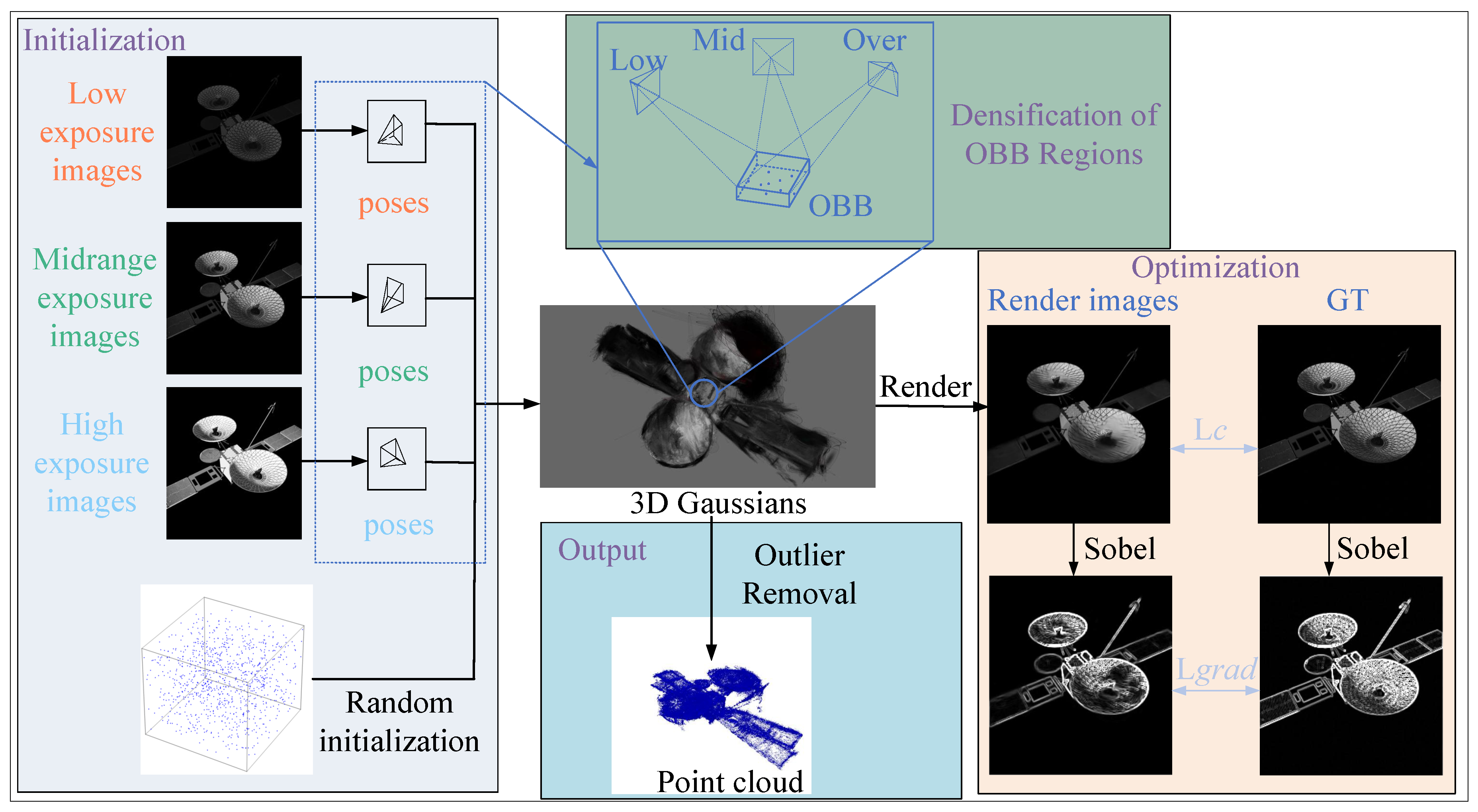
3.1. Overall Framework

Our framework builds on 3DGS. As Figure 1 shows, low-, medium-, and high-exposure images were jointly used as supervision during training. We compute an OBB from the intersection of the three camera-view frusta and selectively densify Gaussians within this zone. A Sobel-based edge loss sharpens high-frequency details, while a centroid-adaptive filter removes outlier primitives from the final model.

3.2. Preliminaries: 3D Gaussian Splatting

Our method adopts 3DGS as its baseline; 3DGS is an emerging neural rendering technique, which, unlike previous NeRF methods, explicitly represents the scene using a large number of anisotropic 3D Gaussian primitives, with each following a 3D Gaussian primitives distribution, which can be expressed as follows:

$$G\left(\mu \right)=e^{-{\displaystyle \frac{1}{2}}{\mu }^T{\Sigma }^{-1}\mu },$$

(1)

where $\mu \in {\mathbb{R}}^3$ denotes the mean (center position) and $\Sigma \in {\mathbb{R}}^{3\times 3}$ represents the covariance matrix (controlling the shape and orientation of the Gaussian).

Additionally, each 3D Gaussian is also characterized by an opacity $\alpha \in \mathbb{R}$ and spherical harmonic (SH) parameters $\mathcal{C}\in {\mathbb{R}}^k$ (where k denotes the degrees of freedom), used for modeling view-dependent color.

To facilitate optimization, the covariance matrix $\Sigma$ can be further represented by a rotation matrix R and a scaling matrix S:

$$\Sigma =RS{S}^T{R}^T.$$

(2)

During the rendering process, given a view transformation matrix W, the 3D Gaussians are projected onto the 2D image plane. The corresponding 2D covariance matrix ${\Sigma }^{\prime }\in {\mathbb{R}}^{2\times 2}$ is given by the following:

$${\Sigma }^{\prime }=JW\Sigma W^T{J}^T,$$

(3)

where J is the Jacobian matrix of the affine approximation of the projective transformation. After projecting the 3D Gaussian primitives onto the 2D plane, the next step is to compute the color for each pixel in the image. For each pixel, the color C is computed by blending the N-ordered 3D Gaussian primitives overlapping it:

$$C=\sum _{i\in N}{c}_i{\alpha }_i\prod _{j=1}^{i-1}(1-{\alpha }_j).$$

(4)

After rendering the image, 3DGS measures the similarity between the rendered image and the ground-truth image via pixel-wise comparison using the $L_1$ and $L_{\mathrm{D}-\mathrm{SSIM}}$ photometric losses:

$$L_{\mathrm{C}}=(1-\lambda )L_1(\mathrm{I},\widehat{\mathrm{I}})+\lambda L_{\mathrm{D}-\mathrm{SSIM}}(\mathrm{I},\widehat{\mathrm{I}}),$$

(5)

where $\lambda$ is a hyperparameter, I denotes the ground-truth image, and $\widehat{I}$ represents the rendered image. In 3DGS, $\lambda$ is set to 0.2, and $L_{\mathrm{D}-\mathrm{SSIM}}$ is the structural similarity index measure (SSIM) loss based on [40].

3.3. Sobel Edge Regularization

The standard 3DGS optimization process primarily relies on pixel-level loss functions (such as $L_1$ and $L_{\mathrm{D}-\mathrm{SSIM}}$) to drive learning. While this approach is generally effective, it mainly enforces photometric consistency, which can sometimes fail to capture fine geometric details, leading to overly smooth surfaces and blurred edges in the reconstruction.

This limitation becomes particularly prominent when processing exposure bracketing image sequences, where severe and inconsistent inter-view brightness variations introduce conflicting supervision signals. Under such conditions, standard pixel-level optimization struggles to preserve high-frequency information and sharp edges, which are especially critical for the reconstruction of man-made space targets. Space targets commonly exhibit distinct structural boundaries, including solar panel outlines, antennae, and object-background silhouettes, which are essential for achieving accurate 3D representations. Pixel-wise losses alone are insufficient to recover these essential geometric cues.

To address this issue, a structure-aware gradient loss based on the Sobel operator is incorporated as a complementary constraint. The Sobel operator, a classical first-order differential filter, enhances sensitivity to high-frequency content by computing intensity differences within a $3\times 3$ neighborhood. This enables the effective extraction of edge features and geometric contours associated with space target structures. Specifically, the Sobel operator employs two $3\times 3$ convolution kernels to estimate image gradients in the horizontal ($S_x$) and vertical ($S_y$) directions, respectively:

$$S_x=\left[\begin{array}{ccc}-1& 0& 1\\ -2& 0& 2\\ -1& 0& 1\end{array}\right]$$

(6)

$$S_y=\left[\begin{array}{ccc}-1& -2& -1\\ 0& 0& 0\\ 1& 2& 1\end{array}\right].$$

(7)

Based on the high-frequency features extracted by the Sobel operator described above, we define the structure-aware gradient loss using the $L_1$ norm as follows:

$$L_{\mathrm{grad}}=\parallel S_x\left(I_{\mathrm{pred}}\right)-S_x\left(I_{\mathrm{gt}}\right){\parallel }_1+{\parallel S_y\left(I_{\mathrm{pred}}\right)-S_y\left(I_{\mathrm{gt}}\right)\parallel }_1,$$

(8)

where $I_{\mathrm{pred}}$ and $I_{\mathrm{gt}}$ represent the rendered image and the ground-truth image, respectively. Our designed gradient loss, by explicitly supervising high-frequency structural information, encourages the reconstruction result to maintain sharp edges and fine surface details.

3.4. Exposure Bracketing OBB Regional Densification

The imaging of space targets presents significant challenges due to highly non-uniform illumination. In the space environment, the absence of atmospheric scattering leads to extreme lighting conditions, where surfaces illuminated by direct sunlight often exhibit a combination of intensely reflective regions and deep shadows. To mitigate this issue and capture scene details across a wide range of brightness levels, exposure bracketing is commonly employed, acquiring images at multiple exposure settings.

However, as described in MVGS [39], the standard 3DGS training strategy follows the convention of selecting only a single image per iteration for supervision, consistent with the NeRF paradigm. While this single-image optimization scheme is generally effective under uniform lighting conditions, it proves inadequate for handling the wide dynamic range introduced by exposure-bracketed image sequences. Although the camera captures rich, complementary information across different exposures, the random selection of a single view of information during training may prevent the model from fully utilizing the multi-exposure data. Consequently, this strategy limits the reconstruction quality in scenes with drastic brightness variations.

3.4.1. Exposure Bracketing Constraint

To address this, we study an exposure bracketing constraint strategy that jointly utilizes multi-exposure data during training. In contrast to the standard 3DGS approach, which selects only a single image per iteration, the proposed method incorporates a triplet of images with different exposure levels, denoted as $\{I_l,I_m,I_h\}$, where l, m, and h represent low, medium, and high exposures, respectively. This design enables the construction of a unified information fusion framework that leverages complementary visual cues under varying illumination conditions, thereby enhancing the robustness and fidelity of the reconstruction.

• Highlight Detail Preservation: The low-exposure image $I_l$ effectively captures texture and edge features in brightly illuminated regions, preventing detail loss due to overexposure that might occur under other exposure conditions.
• Shadow Region Structure Recovery: The high-exposure image $I_h$ reveals structural information within shadow regions, filling in information that is missing in low-exposure conditions due to insufficient brightness.
• Overall Structure Balance Maintenance: The medium-exposure image $I_m$ provides a baseline representation of the object’s overall form, establishing a continuous transition between highlight and shadow regions.

By incorporating images captured under three distinct exposure conditions, the proposed framework enables the optimization process to account for reconstruction quality across varying illumination levels. To this end, a hybrid loss function is defined for each exposure, combining the mean absolute error ($L_1$) and the structural similarity loss ($L_{\mathrm{D}-\mathrm{SSIM}}$), which jointly supervise both pixel-wise brightness accuracy and structural consistency:

$$L_{\mathrm{ME}}=\sum _{e\in \{l,m,h\}}\left((1-{\lambda }_{\mathrm{D}-\mathrm{SSIM}})L_1^e+{\lambda }_{\mathrm{D}-\mathrm{SSIM}}{L}_{\mathrm{D}-\mathrm{SSIM}}^e\right),$$

(9)

where

$$\begin{array}{cc}\hfill L_1^e& \hfill =L_1(I_e,{\widehat{I}}_e)\hfill \end{array}$$

(10)

$$\begin{array}{cc}\hfill L_{\mathrm{D}-\mathrm{SSIM}}^e& \hfill =L_{\mathrm{D}-\mathrm{SSIM}}(I_e,{\widehat{I}}_e).\hfill \end{array}$$

(11)

Here, ${\widehat{I}}_e$ represents the rendered image for exposure level e, and $I_e$ represents the ground-truth image for exposure level e. ${\lambda }_{\mathrm{D}-\mathrm{SSIM}}$ is the weighting coefficient used to balance the two losses, set to 0.2 in our implementation. This multi-exposure synergistic optimization scheme enables the 3D Gaussian primitives to simultaneously adapt their visual appearance under different illumination conditions, enhancing the model’s robustness to illumination variations.

3.4.2. OBB Region Densification

Although the exposure-bracketing constraint facilitates the integration of complementary information across different exposure levels, reliance on a global loss function limits the model’s ability to precisely identify and refine locally underperforming regions. To address this issue, we propose an adaptive OBB region densification mechanism that performs targeted optimization by evaluating local reconstruction quality under varying exposure conditions.

Specifically, we employ a sliding-window strategy to assess local reconstruction performance. In our implementation, this window has fixed dimensions of $h_{box}\times w_{box}$ (specifically, $20\times 40$ pixels). The window slides across each exposure image in a non-overlapping manner, meaning the stride is equal to the window dimensions ($s_h=h_{box}$, $s_w=w_{box}$). For each iteration and each of the three exposure images $\{I_l,I_m,I_h\}$, this process computes the average $L_1$ loss within each $20\times 40$ tile. The single tile exhibiting the maximum average $L_1$ loss is then selected as the “high-loss region” for that specific exposure image, as shown in Figure 2a. Consequently, this yields a set of three distinct high-loss 2D tiles, one from each exposure level (e.g., $T_l,T_m,T_h$). This approach ensures that critical regions from underexposed, correctly exposed, and overexposed parts of the scene are considered for refinement. As a concrete example, if for one of the exposure images (e.g., $I_l$), the $20\times 40$ tile starting at pixel coordinates (row = R, col = C) is identified as the tile with the maximum L1 loss, this specific 2D region, defined by pixel coordinates [R, C, R + 20, C + 40], serves as one of the areas from which four corner rays are cast for subsequent 3D OBB computation.

After identifying the regions requiring refinement, four rays are cast from the vertices of each high-loss region, and their intersections with the scene geometry are used to compute the corresponding 3D spatial volumes, as shown in Figure 2b. This maps problematic 2D regions to 3D space, enabling precise spatial localization for point cloud densification. For better localization, we use OBB instead of an axis-aligned bounding box (AABB), as 3D Gaussian primitives typically exhibit a predominant directional alignment rather than being uniformly distributed.

When identifying regions for densification based on high reconstruction errors, it is essential to accurately bound the anisotropic 3D Gaussian clusters. AABBs, constrained to the global coordinate axes, often result in loose bounds that include empty space or irrelevant primitives within the densification volume.

OBB, in contrast, can align with the natural axes of the data. By applying principal component analysis (PCA) to the 3D means of the Gaussian primitives within the high-loss region, we compute the OBB, providing a tighter, more representative bounding of the primitive distribution. As shown in Figure 3, OBB better conforms to the actual spatial distribution of 3D Gaussian primitives, minimizing redundant space and ensuring a more focused densification process. This alignment significantly reduces computational overhead by eliminating unnecessary volume inclusion and improves the efficiency of the reconstruction process.

From the ray-intersected region, a set of 3D Gaussian primitives is extracted and denoted as $G=\{g_1,g_2,\dots ,g_n\}$, where n is the number of 3D Gaussian primitives within the region and $g_i$ denotes the i-th 3D Gaussian primitive. The average of their means, denoted as $\overline{\mu }$, is computed and used as the center of the corresponding OBB:

$$\overline{\mu }={\displaystyle \frac{1}{n}}\sum _{i=1}^n{\mu }_i,$$

(12)

where ${\mu }_i$ is the mean of the i-th 3D Gaussian primitive distribution, and $\overline{\mu }$ represents the average mean of the 3D Gaussian primitives set G. Then, we subtract the average mean from the mean of each 3D Gaussian primitive distribution in the set G to obtain the set of centered 3D Gaussian primitive means $G^{\prime }=\{\mathbf{M}-\overline{\mu }\}$. Here, $\mathbf{M}$ is the matrix formed by using the means ${\mu }_i$ from G as its row vectors.

Principal component analysis (PCA) [41] is then applied to the centered 3D Gaussian primitives set $G^{\prime }$, from which the covariance matrix C is computed as follows:

$$C={\displaystyle \frac{1}{n-1}}{\mathbf{G}}^{\prime T}{\mathbf{G}}^{\prime },$$

(13)

where ${\mathbf{G}}^{\prime }$ is the matrix whose rows are the centered means (elements of the set $G^{\prime }$). By performing eigenvalue decomposition on the covariance matrix C, we obtain the eigenvalues ${\lambda }_1\ge {\lambda }_2\ge {\lambda }_3$ and the corresponding eigenvectors $v_1,v_2,v_3$. These three eigenvectors define the three principal axis directions of the OBB.

A rotation matrix $\mathbf{R}=[v_1,v_2,v_3]$ is constructed from the eigenvectors to transform coordinates from the world space to the OBB’s local coordinate system. The means of the original 3D Gaussian primitives set G are then projected into this local frame using $\mathbf{R}$:

$$G_{\mathrm{OBB}}=(\mathbf{M}-\overline{\mu })\mathbf{R}.$$

(14)

In the OBB local coordinate system, compute the minimum value ${\min }_{\mathrm{OBB}}$ and maximum value ${\max }_{\mathrm{OBB}}$ of the transformed 3D Gaussian primitives means $G_{\mathrm{OBB}}$ along each coordinate axis. The half-extents (half-length, half-width, half-height) h of the OBB are then calculated using the following formula:

$$h={\displaystyle \frac{{\max }_{\mathrm{OBB}}-{\min }_{\mathrm{OBB}}}{2}}.$$

(15)

Finally, the OBB is defined by the center $\overline{\mu }$, the rotation matrix $\mathbf{R}$, and the half-extents h, denoted as $(\overline{\mu },\mathbf{R},h)$. This region tightly encloses the 3D Gaussian primitives within high-loss areas, providing a well-bounded spatial extent for targeted densification. The original 3DGS densification strategy is subsequently applied within each identified OBB region.

3.5. Initialization and Optimization

In the reconstruction of unknown space targets, one major challenge is the absence of an initial point cloud. Due to the severe illumination imbalance commonly observed in spaceborne optical imagery, traditional SfM pipelines, such as COLMAP [15], often fail to produce reliable camera poses and initial 3D structures. To address this, we adopt a random initialization strategy by generating 100,000 3D Gaussian primitives uniformly distributed in 3D space. Camera poses are instead derived from precise orbital parameters.

During optimization, we follow the Gaussian splitting and cloning threshold strategy introduced in Pixel-GS [42]. To achieve high-fidelity reconstruction, two core components—Sobel edge regularization and OBB region densification—are integrated into a unified optimization framework. The overall loss function is defined as follows:

$$L_{\mathrm{total}}=\sum _{e\in \{l,m,h\}}\left((1-{\lambda }_{\mathrm{D}-\mathrm{SSIM}})L_1^e+{\lambda }_{\mathrm{D}-\mathrm{SSIM}}{L}_{\mathrm{D}-\mathrm{SSIM}}^e+{\lambda }_{\mathrm{grad}}{L}_{\mathrm{grad}}\right),$$

(16)

where ${\lambda }_{\mathrm{grad}}$ is the hyperparameter used to balance the weight of the gradient loss, which we set to 0.2 here.

Our overall optimization is guided by the total loss function, $L_{\mathrm{total}}$, which combines the $L_{\mathrm{ME}}$ loss for handling multi-exposure images and the $L_{\mathrm{grad}}$ loss for enhancing edges. In each optimization step, the gradients from $L_{\mathrm{total}}$ simultaneously drive two key processes. The first process involves updating the parameters of existing 3D Gaussian primitives. The second process guides the OBB region densification strategy Section 3.4. Specifically, when $L_{\mathrm{total}}$, particularly its $L_{\mathrm{ME}}$ component, indicates that certain regions are poorly reconstructed due to exposure issues, the OBB densification mechanism is activated to strategically add new Gaussian primitives in these areas. This can be conceptualized as supplying more “modeling material” where details are lacking. Concurrently, the Sobel edge loss $L_{\mathrm{grad}}$ (see Section 3.3), also part of $L_{\mathrm{total}}$, continuously acts on all 3D Gaussian primitives in the scene, both pre-existing and newly added ones. The role of $L_{\mathrm{grad}}$ is to ensure these “modeling materials” are finely organized to form sharp object edges and rich surface details. Thus, OBB region densification provides the model with the necessary expressive capacity to capture fine features under complex illumination, while Sobel edge regularization ensures these features are rendered in a structurally clear and edge-sharpened manner. These two modules work synergistically under the unified framework of $L_{\mathrm{total}}$; densification provides the foundational substance, and edge regularization refines this substance, collectively enhancing the final quality of the 3D reconstruction of space targets. In the final stage of optimization, a center-constrained adaptive algorithm is employed to eliminate outliers.

4. Dataset

Due to the high costs and technical challenges associated with acquiring real-world space target data, publicly available datasets remain scarce. Existing resources, such as SPEED+ [43] and SHIRT [44], primarily consist of synthetic images rendered using professional software or images captured under controlled laboratory conditions. However, current simulation datasets that provide ground-truth camera poses typically assume fixed exposure settings, which fail to reflect the high dynamic range conditions encountered in real-world scenarios.

To address this limitation, we present the orbital bracketing reconstruction dataset for space targets (OBR-STs), a new physics-based synthetic dataset designed for the 3D reconstruction of space targets under exposure bracketing. Constructed using the Blender rendering engine, OBR-ST simulates realistic rendezvous trajectories derived from two-line element (TLE) data, while incorporating varying exposure levels to mimic camera bracketing in orbit. Crucially, the dataset provides precise camera poses synchronized with rendered images in a format compatible with modern NeRF and 3DGS frameworks.

An overview of the data generation workflow is shown in Figure 4. The inputs include a 3D model of the space target and TLE information for both the chaser and the target. First, orbital dynamics are computed to determine the relative pose of the chaser with respect to the target, as well as the position of the Sun at each time step. These parameters are then fed into Blender, where the camera pose of the chaser and the lighting conditions are configured to simulate the space environment. Rendered images with Gaussian noise are rendered using periodic exposure variations (low, medium, and high). This process is repeated across time steps to simulate a natural fly-around trajectory. The resulting dataset comprises a sequence of multi-exposure images paired with their corresponding ground-truth camera poses.

4.1. Simulation Inputs

Figure 4 provides a schematic overview of our dataset generation process, highlighting the key steps involved. The pipeline requires two primary inputs: a 3D model of the target and the corresponding TLE information for both the chaser and the target.

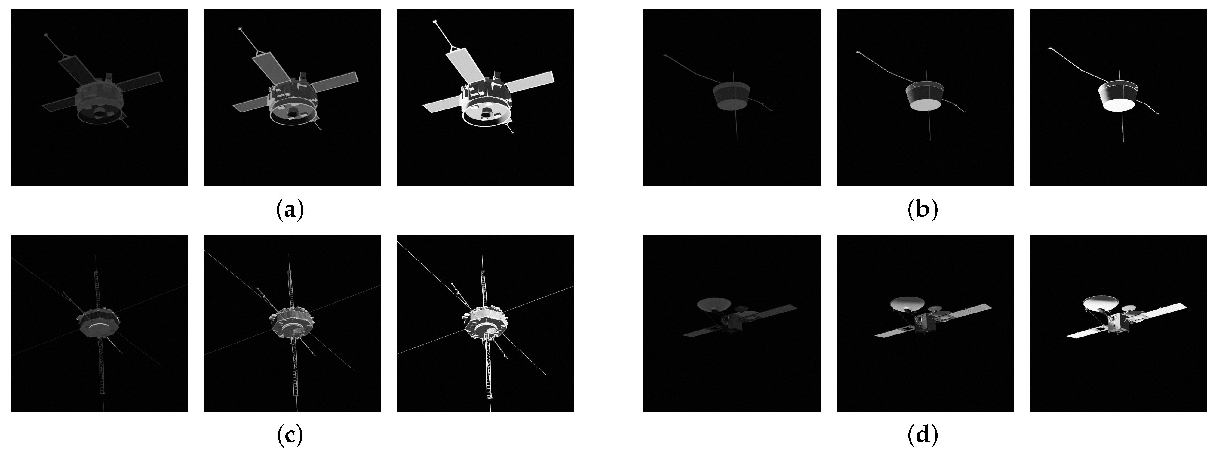
• Space target model: We acquire six distinct space target models from NASA’s publicly available 3D model repository. These models are uniformly processed by converting them into the .obj format for subsequent import into the Blender software. Furthermore, we utilize the corresponding material properties available on the NASA website to ensure visual fidelity.
• Orbital information (TLE): We configure a simulation scenario featuring a natural fly-around trajectory. From this scenario, we extract the corresponding TLE data for the chaser and the target during the simulated rendezvous phase.

4.2. Blender Rendered Images

Given the input 3D model and TLE data of the corresponding space target, the Blender scene is rendered according to the following procedures:

• Scene setup: The Blender camera is designated as the chaser and the imported 3D model represents the target. To reflect the visual characteristics of outer space, the scene background is set to black.
• Illumination: To accurately compute the Sun’s position relative to both space targets, we use the ephemeris file de421.bsp, provided by NASA’s Jet Propulsion Laboratory (JPL). The resulting solar vector is used to position and orient the primary light source (implemented as a sun or planar lamp) within Blender, simulating directional solar illumination.
• Relative pose: The relative position and attitude of the chaser with respect to the target are dynamically updated at each time step based on orbital calculations derived from the input TLE data.
• Exposure variation: To replicate exposure bracketing used in real onboard imaging systems, we periodically vary the camera’s exposure settings across consecutive frames, cycling through low—0.05 ms, medium—0.1 ms, and high—0.2 ms exposure levels.
• Noise simulation: Gaussian noise is added to the rendered images to emulate noise.

4.3. Simulation Output

By iteratively executing the procedures described in Section 4.2, we simulated observations at multiple time instances, generating multi-view image sequences that followed a natural fly-around trajectory. The dataset comprises six distinct space target models. For each model, a total of 363 images with a resolution of 800 × 800 pixels were generated (as illustrated in Figure 5).

Following the established directory structure of the NeRF Synthetic dataset, each 363-frame sequence was precisely divided as follows: 198 images were allocated to the training set, 66 images to the validation set, and 99 images to the test set. Importantly, each image was paired with precise ground-truth camera pose information, ensuring the dataset’s direct applicability to training and evaluating mainstream neural rendering frameworks. It is crucial to note that the validation set was exclusively utilized within the original NeRF training pipeline. For all comparative methods, including 3DGS, training and evaluation were conducted solely using the training and test sets to ensure fair and consistent performance comparisons.

5. Experiments and Results

We conducted a series of experiments on the proposed OBR-ST dataset, as well as the publicly available SHIRT dataset, to compare our method with existing approaches. Both qualitative and quantitative analyses were carried out to validate the effectiveness of the proposed method.

5.1. Datasets

We employed two datasets for evaluation in our experiments, that is, the custom-built OBR-ST dataset and the publicly available SHIRT pose estimation dataset.

• OBR-ST dataset: This task-specific dataset contains six distinct space target models. Each model is depicted in 363 images, split into 198 training, 99 test, and 66 validation samples. The dedicated validation split supports the training regime of NeRF-based methods for orbital targets.
• SHIRT dataset: For the publicly available SHIRT dataset, we adopted a processing strategy similar to that used for OBR-ST. We selected the first 363 images from each category and divided them (per category) into 198 training images, 99 test images, and 66 validation images. The original camera pose information was converted into a format compatible with the NeRF synthetic dataset conventions, enabling direct integration into NeRF training pipelines.

5.2. Implementation Details

Our method builds upon the original implementation of 3DGS, integrating the core methodologies presented in Section 3.3 and Section 3.4 into the 3DGS framework, while preserving all default hyperparameters. Specifically, the learning rates were set as follows: 0.0025 for SH features, 0.05 for opacity adjustments, 0.005 for scaling operations, and 0.001 for rotation transformations. We employed the Adam optimizer for training and conducted 30,000 iterations uniformly across all experiments.

For a comprehensive comparison, we adopted 3DGS as our primary baseline and included MVSNet [45], NeRF, Pixel-GS, and MVGS as additional comparison methods. For 3DGS and its variants (including our method, Pixel-GS, and MVGS), we trained on the training set of each dataset and evaluated on the corresponding test set. In contrast, NeRF was trained on the combined training and validation sets and evaluated on the test set. The MVSNet evaluation was performed directly using the officially provided pre-trained model for inference. Regarding implementation details, 3DGS and its variants were based on their respective official open-source codebases.

All experiments were conducted on a workstation with the following specifications:

• Processor: Intel® Core™ i9-14900KS @ 3.20 GHz (14th gen)
• Graphics Processing Unit (GPU): NVIDIA GeForce RTX 4090 with 24 GB GDDR6X memory
• Memory: 64 GB

The software environment was configured as follows:

• Operating System: Ubuntu 20.04
• Deep Learning Framework: PyTorch 2.0.0, with CUDA 11.8

5.3. Evaluation Metrics

To comprehensively evaluate the reconstruction performance of our method, we assess it based on two primary aspects, that is, texture reconstruction quality and geometric structure accuracy.

For texture reconstruction quality, we employed three widely-used image quality assessment metrics:

Peak signal-to-noise ratio (PSNR) quantifies the fidelity of the reconstructed image from the perspective of pixel error. A higher PSNR value indicates a smaller mean squared error between the reconstructed and ground-truth images, signifying better image quality. Its calculation formula is:

$$\mathrm{PSNR}=10·{\log }_{10}\left({\displaystyle \frac{{\mathrm{MAX}}_I^2}{\mathrm{MSE}}}\right),$$

(17)

where ${\mathrm{MAX}}_I$ represents the maximum possible pixel intensity value, and MSE denotes the mean squared error between the original and reconstructed images.

Structural similarity index measure (SSIM) measures the similarity between two images by comprehensively evaluating luminance, contrast, and structural information. A higher SSIM value indicates that the reconstructed image is perceptually closer to the ground-truth image. It is typically calculated based on the following form:

$$\mathrm{SSIM}(x,y)=\left[l{(x,y)}^{\alpha }·c{(x,y)}^{\beta }·s{(x,y)}^{\gamma }\right],$$

(18)

where $l(x,y)$ represents luminance similarity, $c(x,y)$ represents contrast similarity, and $s(x,y)$ represents structural similarity. The terms $\alpha$, $\beta$, and $\gamma$ in the formula are weighting factors.

Learned perceptual image patch similarity (LPIPS) utilizes features extracted by deep neural networks to compute the perceptual distance between images. It is considered to better simulate the perceptual characteristics of the human visual system. A lower LPIPS value indicates that the reconstructed image is visually more consistent with the ground-truth image. Its calculation formula is as follows:

$$\mathrm{LPIPS}(x,y)=\sum _l{\displaystyle \frac{1}{H_l{W}_l}}\sum _{h,w}{∥w_l\odot \left({\widehat{f}}_{hw}^l\left(x\right)-{\widehat{f}}_{hw}^l\left(y\right)\right)∥}_2^2,$$

(19)

where $f^l\left(x\right)$ and $f^l\left(y\right)$ represent the feature maps extracted from images x and y at layer l of the network. $\widehat{f}$ denotes the normalized features. $w_l$ are the learnable channel-wise weighting coefficients for each layer. $H_l$ and $W_l$ represent the spatial dimensions of the feature map at layer l. ⊙ denotes element-wise multiplication across channels.

For geometric structure accuracy, our objective is to comprehensively evaluate the consistency between the reconstructed point cloud and the ground-truth point cloud from the key perspectives of accuracy and completeness. To this end, we selected the following complementary metrics:

Chamfer distance (CD) primarily measures the overall similarity between two point clouds $P_1={\{x_i\in {\mathbb{R}}^3\}}_{i=1}^n$ and $P_2={\{x_j\in {\mathbb{R}}^3\}}_{j=1}^m$ by calculating the bidirectional average distance between them. A lower CD value indicates that the reconstructed and ground-truth point clouds are closer, implying a smaller geometric error. It comprehensively reflects both the accuracy and completeness of the reconstruction. Its calculation is as follows:

$$\mathrm{Chamfer}(P_1,P_2)={\displaystyle \frac{1}{2n}}\sum _{i=1}^n\parallel x_i-\mathrm{NN}(x_i,P_2)\parallel +{\displaystyle \frac{1}{2m}}\sum _{j=1}^m\parallel x_j-\mathrm{NN}(x_j,P_1)\parallel ,$$

(20)

where $\mathrm{NN}(x,P)=\arg {\min }_{x^{\prime }\in P}\parallel x-x^{\prime }\parallel$ is the nearest neighbor function, using the Euclidean norm $\parallel ·\parallel$.

Hausdorff distance (HD) is another metric used for measuring the discrepancy between two point sets (point clouds), focusing on the maximum nearest-neighbor distance between them, i.e., the worst-case deviation. HD is particularly sensitive to large local errors or outliers (affecting accuracy). A lower HD value indicates that the two point clouds are sufficiently close even in the most mismatched regions, reflecting good control over boundaries and outliers in the reconstruction result. Its calculation is as follows:

$$\mathrm{Hausdorff}(P_1,P_2)={\displaystyle \frac{1}{2}}\underset{x\in P_1}{\max }\parallel x-\mathrm{NN}(x,P_2)\parallel +{\displaystyle \frac{1}{2}}\underset{x^{\prime }\in P_2}{\max }\parallel x^{\prime }-\mathrm{NN}(x^{\prime },P_1)\parallel ,$$

(21)

where $\mathrm{NN}(·,·)$ is the nearest neighbor function as defined for CD, and $\parallel ·\parallel$ is the Euclidean norm.

Completeness percentage directly quantifies the extent to which the reconstructed point cloud $P_{\mathrm{Rec}}={\{y_j\in {\mathbb{R}}^3\}}_{j=1}^m$ covers the ground-truth point cloud $P_{\mathrm{GT}}={\{x_i\in {\mathbb{R}}^3\}}_{i=1}^n$, assessing whether the reconstruction has captured the complete geometric shape of the target. A higher value (approaching 100%) indicates a more complete reconstruction. Its calculation is as follows:

$$\mathrm{Completeness}(P_{\mathrm{GT}},P_{\mathrm{Rec}},\tau )={\displaystyle \frac{1}{|P_{\mathrm{GT}}|}}\sum _{x\in P_{\mathrm{GT}}}I\left(\underset{y\in P_{\mathrm{Rec}}}{\min }\parallel x-y\parallel <\tau \right),$$

(22)

where ${\min }_{y\in P_{\mathrm{Rec}}}\parallel x-y\parallel$ represents the minimum Euclidean distance from a ground-truth point x to any point in the reconstructed point cloud $P_{\mathrm{Rec}}$. $\tau$ is a predefined distance threshold, set to 0.01 in our case. $I\left(·\right)$ denotes the indicator function, which is 1 if the condition in the parentheses is true, and 0 otherwise. $|P_{\mathrm{GT}}|$ is the number of points in the ground-truth point cloud.

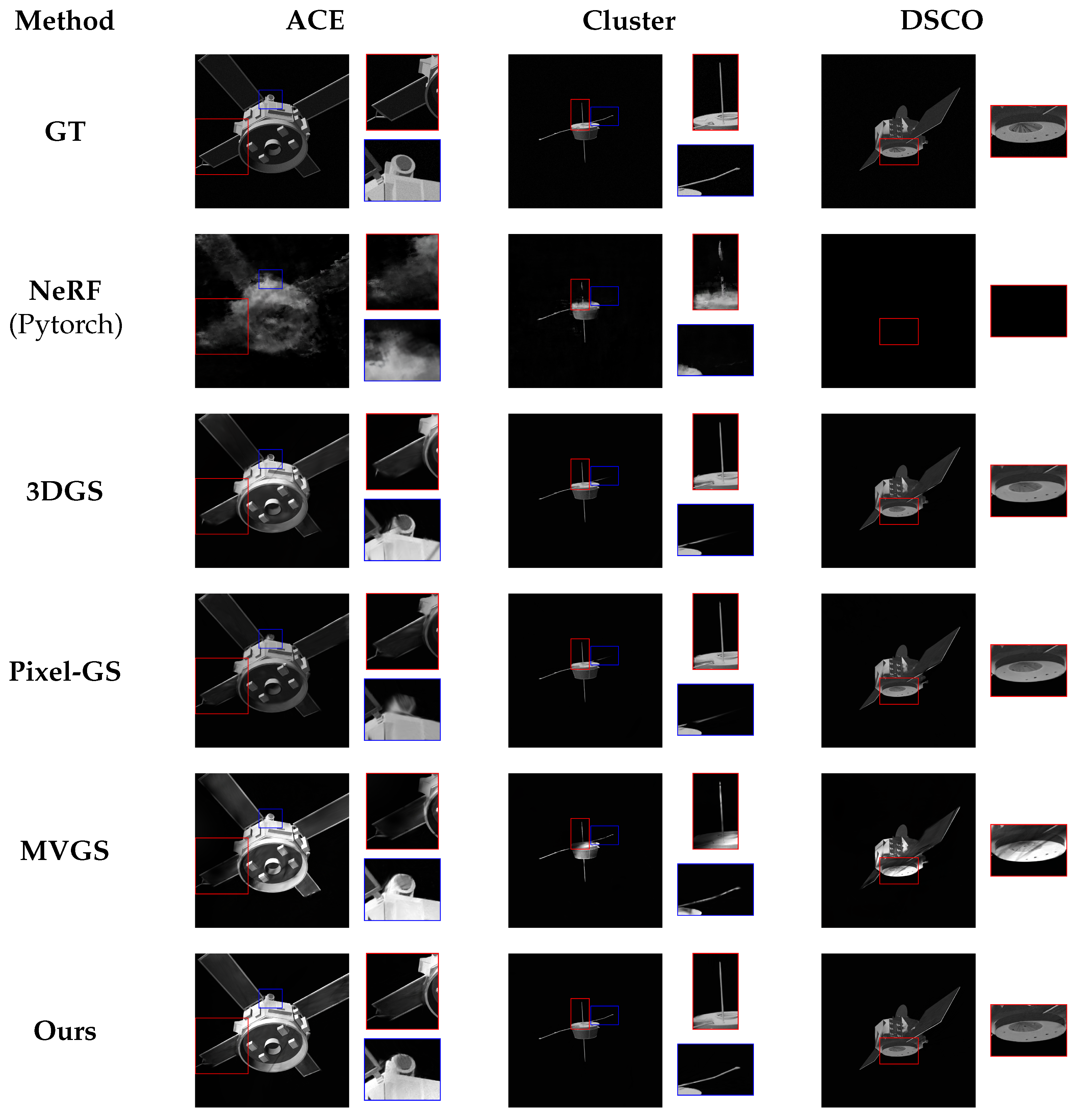
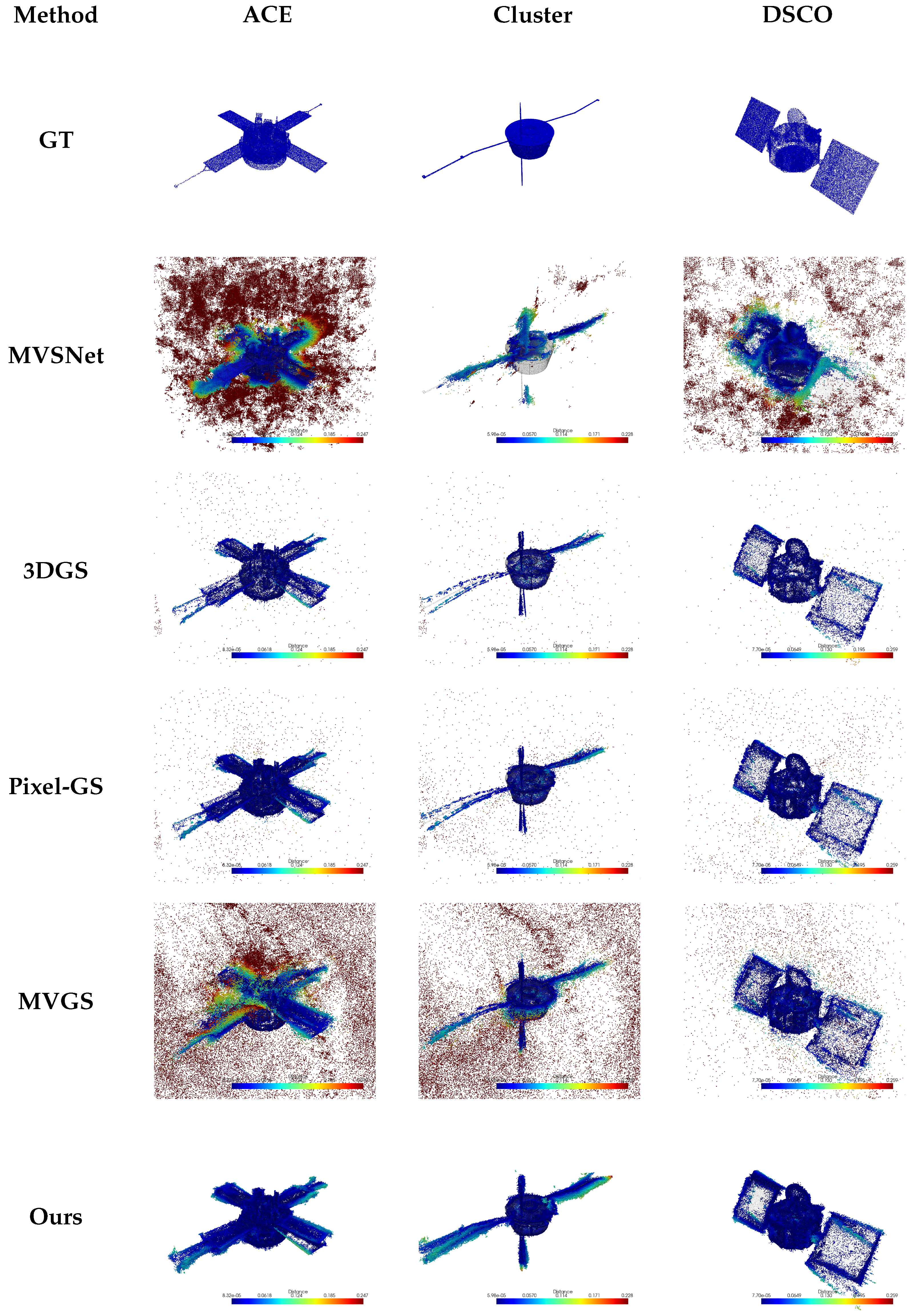
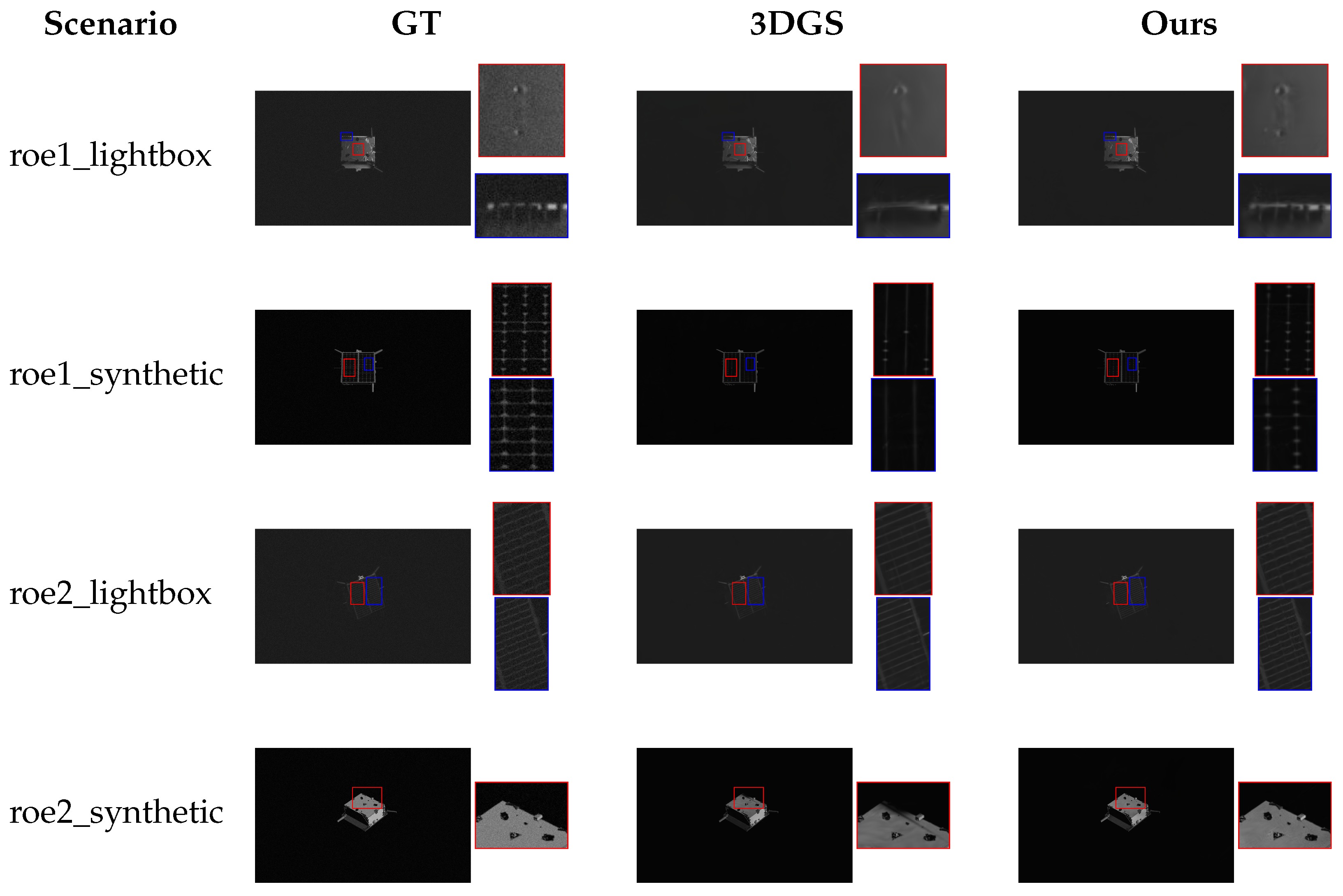
5.4. Qualitative Comparison

We first conduct a qualitative evaluation on the OBR-ST dataset to visually assess the reconstruction performance of our method. The evaluation focuses on two key aspects, namely, texture quality and geometric structure accuracy, comparing our approach with several baseline and state-of-the-art methods. Specifically, to evaluate texture reconstruction quality, we render novel view images from the test set and visually compare the results with those generated by NeRF, 3DGS, Pixel-GS, and MVGS. For geometric structure accuracy, we compare the reconstructed outputs from MVSNet, 3DGS, Pixel-GS, and MVGS. It is important to note that NeRF is excluded from the geometric accuracy comparison, as standard implementations do not provide a straightforward means of extracting explicit point clouds from its implicit volumetric representation.

As illustrated in Figure 6, we present the visualized reconstruction results for three space target models using different methods. The results show that the NeRF method performs poorly when processing the exposure bracketing image dataset used in this study. Among the three models presented, one fails to render correctly, resulting in a complete rendering failure (black background with no shape recovery). The other two models, although rendered, suffer from blurriness, incomplete reconstruction of numerous components, and low overall detail fidelity. Similarly, the original 3DGS and its pixel-level variants blur fine parts because exposure fluctuations corrupt per-Gaussian color estimates, causing over-smoothing. In contrast, our proposed method demonstrates superior performance in detail recovery compared to the original 3DGS, its variants, and NeRF. For the cluster model, our method successfully renders the thin elongated structure on the target’s right side. This feature is either missing or significantly under-detailed in the reconstructions produced by other methods. This enhanced detail recovery mainly comes from two factors. First, the joint use of low-, medium-, and high-exposure images lets the 3DGS see both highlight and shadow information in every iteration, so fine textures are retained instead of being clipped by over- or under-exposure. Second, the Sobel-based edge loss adds an explicit penalty on blurred boundaries, forcing Gaussians to align with sharp structural edges. These two mechanisms act together to curb color drift, focus capacity on high-frequency regions, and ultimately raise the fidelity of the reconstructed details.

Figure 7 shows the geometric structure results for the same three models used in the texture quality assessment. We present an example ground-truth point cloud for each model. In the comparison images for each method, the ground-truth point cloud appears in gray, while the reconstructed point cloud is colored based on its distance to the nearest ground-truth point. Colors closer to blue indicate smaller distances and higher accuracy, while colors closer to red indicate larger distances and lower accuracy. Through comparison, it is evident that our method achieves the best results among the evaluated approaches. MVSNet shows the weakest reconstruction performance, introducing significant noise. A detailed comparison also reveals that MVSNet performs worse than 3DGS in terms of completeness. For example, in the Cluster model, the main body of the space target is poorly reconstructed by MVSNet, with the lower section almost entirely missing. Additionally, the MVGS reconstruction introduces a considerable amount of noise. In comparison, our method produces the least noise, achieves relatively high completeness, and generates fewer outliers. This advantage stems from two key components: firstly, the OBB-guided regional densification adds Gaussians precisely where reconstruction errors are largest, boosting local coverage and overall completeness; secondly, the Sobel edge regularization combined with centroid-adaptive filtering sharpens true boundaries and eliminates isolated or low-opacity points, thereby reducing outliers.

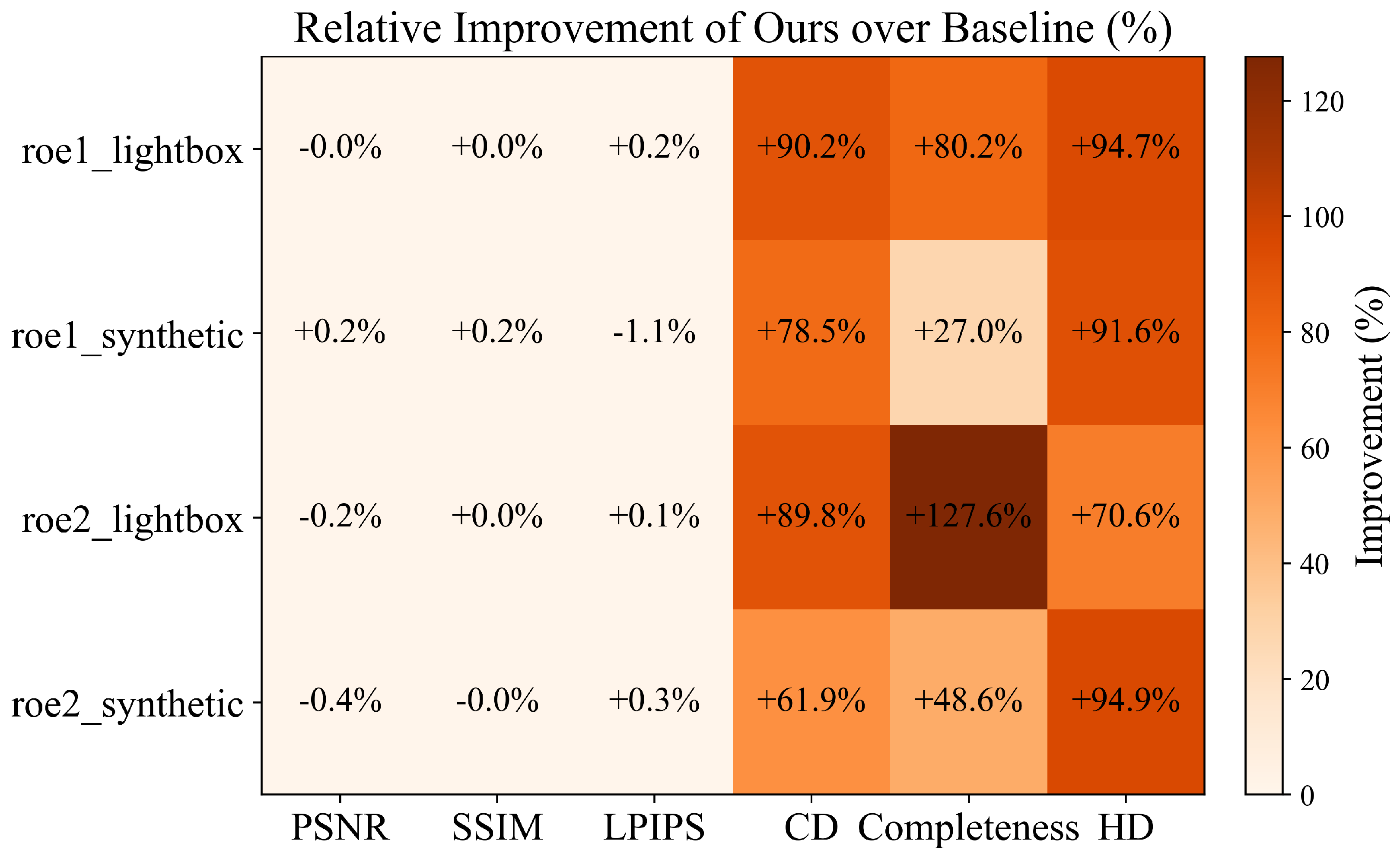
5.5. Quantitative Comparison

To evaluate the performance of our proposed method on the OBR-ST dataset, we compare the same methods used in the qualitative analysis. We first evaluate the texture reconstruction quality using the above metrics PSNR, SSIM, and LPIPS, as described in Section 5.3. Scores are calculated by comparing novel view images rendered by the trained models with the ground-truth images from the test set, with detailed results shown in

Table 1. Performance on the OBR-ST dataset using the PSNR↑ metric. Best (highest), second best, and third best values are highlighted in red, orange, and yellow, respectively. The best value is also bolded.

Module	NeRF (Pytorch)	3DGS	Pixel-GS	MVGS	Ours
ACE	23.5424	26.0240	25.9689	23.4592	26.2057
Cluster	25.8187	28.1415	28.1223	27.8028	28.5121
DSCO	21.0549	28.5198	28.5737	27.7245	28.5951
MM	23.5226	29.2306	29.3822	28.1745	29.6908
SHO	20.6217	23.0715	23.2382	20.4337	23.4519
TDRS	0.3025	25.3843	25.4555	24.1252	25.7606
Average	19.1438	26.7286	26.7902	25.6850	27.0361

,

Table 2. Performance on the OBR-ST dataset using the SSIM↑ metric. Best (highest), second best, and third best values are highlighted in red, orange, and yellow, respectively. The best values are also bolded.

Module	NeRF (Pytorch)	3DGS	Pixel-GS	MVGS	Ours
ACE	0.6777	0.8332	0.8340	0.8080	0.8341
Cluster	0.7421	0.8485	0.8486	0.8443	0.8494
DSCO	0.4950	0.8337	0.8337	0.8280	0.8341
MM	0.5267	0.8415	0.8430	0.8354	0.8461
SHO	0.6115	0.7663	0.7681	0.7155	0.7681
TDRS	0.0329	0.8201	0.8206	0.8033	0.8241
Average	0.5143	0.8239	0.8247	0.8085	0.8260

and

Table 3. Performance on the OBR-ST dataset using the LPIPS↓ metric. Best (lowest), second best, and third best values are highlighted in red, orange, and yellow, respectively. The best value is also bolded.

Module	NeRF (Pytorch)	3DGS	Pixel-GS	MVGS	Ours
ACE	0.5058	0.4797	0.4783	0.4932	0.4731
Cluster	0.4890	0.4812	0.4805	0.4808	0.4776
DSCO	0.5272	0.4859	0.4846	0.4870	0.4821
MM	0.5297	0.4767	0.4723	0.4819	0.4646
SHO	0.5540	0.4931	0.4878	0.5179	0.4737
TDRS	0.8245	0.4810	0.4790	0.4836	0.4697
Average	0.5717	0.4829	0.4804	0.4874	0.4735

.

Analysis of the averaged results (last row of each table) reveals that our method achieves the best performance across all three metrics. This demonstrates that, compared to the baseline methods, our approach generates novel view renderings that are generally closer to the ground-truth images, reflecting superior texture reconstruction quality for the space targets.

Specifically, our method leads in the PSNR metric (Table 1), which measures pixel-level fidelity, achieving an average value of 27.0361, surpassing all other methods. At the same time, for the LPIPS metric (Table 3), which measures perceptual similarity, our method also obtains the best average score (lower is better) of 0.4735. This shows that our method not only achieves higher pixel-level accuracy but also produces images that are perceptually closer to the ground truth. For example, on the SHO model, our method yields a significant improvement over the baseline 3DGS, with an approximate 1.65% increase in PSNR (23.4519 vs. 23.0715) and a 3.93% decrease in LPIPS (0.4737 vs. 0.4931).

Furthermore, regarding the SSIM metric (Table 2), which assesses structural similarity, our method achieves the highest average score (0.8260), indicating superior preservation of structural information. When combined with the PSNR and LPIPS results, these findings demonstrate that our method excels in pixel fidelity, structural preservation, and perceptual quality, providing strong evidence of its effectiveness in enhancing texture reconstruction.

Subsequently, we conduct a quantitative evaluation focused on geometric structure, using CD, HD, and completeness percentage as the primary metrics. NeRF is excluded from this comparison due to its implicit nature, as the official implementation does not provide a standard method for converting the representation into an explicit point cloud. We include MVSNet in the comparison, alongside 3DGS, Pixel-GS, and MVGS. The quantitative results for our method and the baselines are presented in

Table 4. Performance on the OBR-ST dataset using the CD↓ metric. Best (lowest), second best, and third best values are highlighted in red, orange, and yellow, respectively. The best value is also bolded.

Module	MVSNet	3DGS	Pixel-GS	MVGS	Ours
ACE	0.4098	0.1445	0.1206	0.7274	0.0283
Cluster	0.1269	0.2192	0.2345	0.8368	0.0426
DSCO	0.3722	0.1372	0.1510	0.2285	0.0314
MM	0.3439	0.1843	0.1520	0.5305	0.0419
SHO	0.2204	0.0807	0.0852	0.4972	0.0773
TDRS	0.2816	0.1129	0.1218	0.6108	0.0374
Average	0.2925	0.1465	0.1442	0.4774	0.0431

,

Table 5. Performance on the OBR-ST dataset using the completeness percentage↑ metric. Best (highest), second best, and third best values are highlighted in red, orange, and yellow, respectively. The best value is also bolded.

Module	MVSNet	3DGS	Pixel-GS	MVGS	Ours
ACE	40.6683	60.3806	76.4285	58.7431	87.5466
Cluster	14.7993	51.5432	59.1408	66.5348	78.1119
DSCO	31.6447	47.7257	55.4674	59.2630	66.6131
MM	38.1166	71.9740	81.2636	76.8022	91.5039
SHO	20.4281	22.1142	29.9984	26.5029	36.7657
TDRS	48.0172	45.5344	56.8314	61.4799	72.1282
Average	32.2790	49.8787	59.8550	61.6677	72.1116

and

Table 6. Performance on the OBR-ST dataset using the HD↓ metric. Best (lowest), second best, and third best values are highlighted in red, orange, and yellow, respectively. The best value is also bolded.

Module	MVSNet	3DGS	Pixel-GS	MVGS	Ours
ACE	1.6787	4.1167	3.1101	3.6667	0.1361
Cluster	0.9062	3.5868	2.9471	3.8028	0.2404
DSCO	1.6141	3.3337	3.5116	4.3244	0.1619
MM	1.3774	3.7419	2.6208	2.9278	0.3942
SHO	1.0621	2.3937	3.0082	4.0570	1.2159
TDRS	1.6926	3.3094	3.2736	3.6618	0.8767
Average	1.3885	3.4137	3.0786	3.6200	0.5042

.

Analyzing the average results (last row of each table), our method demonstrates significant advantages across all three geometric accuracy metrics. The lowest average CD value (0.0431, Table 4) indicates that our reconstructed point clouds most closely match the ground truth in terms of overall shape and distribution. This performance is notably better than all other methods, including the next-best Pixel-GS (0.1442) and the baseline 3DGS (0.1465), directly reflecting the superior overall accuracy and fidelity of our geometric reconstruction.

For the HD metric (Table 6), which measures the worst-case deviation, our method again achieves the lowest average value (0.5042), substantially outperforming Pixel-GS (3.0786) and 3DGS (3.4137). This suggests that our approach better controls large local errors, resulting in sharper geometric boundaries and fewer outliers. Moreover, for the completeness percentage metric (Table 5), which directly evaluates the coverage of the reconstruction, our method achieves the highest average percentage (72.11%), significantly exceeding MVGS (61.67%) and Pixel-GS (59.86%). This shows that our reconstructions most effectively cover the ground-truth surface, capturing a more complete geometric representation.

Taken together, the results across these three complementary geometric metrics provide strong quantitative evidence of the effectiveness of our method in generating high-accuracy and high-completeness 3D geometric structures, representing a significant advancement over the compared existing approaches.

5.6. Ablation Study

To independently validate the effectiveness of the two core components proposed in our method, namely, Sobel edge regularization (Section 3.3) and exposure bracketing OBB regional densification (Section 3.4), we conduct a series of ablation experiments. Using the original 3DGS as the baseline, we evaluate the impact of adding each component individually, as well as incorporating both components simultaneously (denoted as “ALL”). All experiments are conducted on the OBR-ST dataset, following the same training strategy and parameter settings for 30,000 iterations. Performance is assessed using the following six metrics: PSNR, SSIM, and LPIPS (for texture quality), CD, completeness percentage, and HD (for geometric accuracy). The overall average results are summarized in

Table 7. Average values across six metrics on the OBR-ST dataset, comparing the baseline (3DGS) with the addition of individual components and both components (ALL). The best, second best, and third best values in each column are highlighted in red, orange, and yellow, respectively. The best value is also bolded. ↑ indicates higher values are better, while ↓ indicates lower values are better.

Structure	PSNR↑	SSIM↑	LPIPS↓	CD↓	Completeness Percentage ↑	HD↓
3DGS (Baseline)	26.7286	0.8239	0.4829	0.1465	49.8787	3.4137
+Sobel	26.8931	0.8248	0.4783	0.0416	66.7511	0.3824
+OBB	26.8282	0.8248	0.4765	0.0396	66.5106	0.5884
ALL (Ours)	27.0361	0.8260	0.4735	0.0431	72.1116	0.5042

.

The results in Table 7 clearly show that adding either Sobel edge regularization or exposure bracketing OBB regional densification leads to consistent improvements over the original 3DGS baseline. This demonstrates that each component contributes effectively on its own.

When both components are applied together (denoted as "ALL" in Table 7), the method achieves the best overall performance across all texture quality and geometric accuracy metrics. This outcome highlights the complementary strengths of the two components and their combined contribution to high-quality reconstruction.

Notably, the CD and HD values for our complete method ("ALL") are slightly higher, which indicates marginally lower performance on these specific metrics compared to the best results achieved by adding only OBB densification (CD: 0.0396, "+OBB" row) or only Sobel regularization (HD: 0.3824, "+Sobel" row). We interpret this as a reasonable trade-off in the pursuit of greater completeness. During reconstruction, prioritizing completeness by actively filling potential gaps may lead to a small number of points deviating slightly from the ideal surface, which can result in a modest reduction in CD and HD performance. Given that our final method ("ALL") achieves the best overall results across both texture quality and geometric accuracy, we consider this trade-off acceptable and justified.

5.7. Evaluation on SHIRT Dataset

To further assess the generalization capability of our method, we conducted additional experiments on the publicly available SHIRT dataset, which was designed for pose estimation tasks. The SHIRT dataset consists of images from two simulated low Earth orbit (LEO) rendezvous trajectories, referred to as ROE1 and ROE2. Each trajectory provides two types of image sources, namely, synthetic images rendered with OpenGL and “lightbox” images captured in the terrestrial TRON laboratory. A key difference from our OBR-ST dataset is that the SHIRT dataset uses fixed exposure settings during image acquisition.

For the experimental setup, we followed the dataset partitioning strategy described in Section 5.1. The training procedure used the same default parameters and approach as in the OBR-ST experiments, with a total of 30,000 training iterations. We adopted the same evaluation metrics as before, including PSNR, SSIM, and LPIPS for texture quality, as well as CD, the completeness percentage, and HD for geometric accuracy.

Figure 8 presents a heatmap of relative percentage improvements of our method over the 3DGS baseline on SHIRT. Each cell “+x.x%” shows how much our approach gains (or loses) on each metric in each scenario.

Analysis of the results reveals that our method demonstrates significant superiority in terms of geometric reconstruction accuracy. As shown in Figure 8, all three geometric metrics (CD, completeness percentage, and HD) exhibit substantial positive gains over the baseline. On average, completeness increases by 70.85%, HD error decreases by ≈87.95%, and CD error is reduced by several tens of percent across all four test scenarios. This clearly evidences that our method has a distinct advantage in generating more accurate and complete spatial structures, and that this advantage generalizes to different types of data.

Regarding texture quality, the two methods remain closely matched. The heatmap cells for PSNR, SSIM, and LPIPS all lie within ±0.2% of zero, indicating a negligible change in rendering fidelity. We attribute this to the constant-exposure setting of the SHIRT dataset. Our OBB-densification strategy is specifically designed to exploit exposure variations, so when exposure is fixed, it yields less visible benefit. Nevertheless, matching the baseline under these conditions still demonstrates the robustness of our approach.

For a more intuitive evaluation, qualitative comparison results are presented in Figure 9 and Figure 10. Observing the rendered images in Figure 9, our method demonstrates superior performance in reconstructing space target details and edge sharpness. This improvement benefits from the Sobel edge regularization and our OBB densification strategy. The point cloud visualizations in Figure 10 clearly corroborate the quantitative analysis. Compared to 3DGS, the point clouds generated by our method are noticeably denser, morphologically more complete, and exhibit significantly fewer outliers and noise.

6. Conclusions

This paper investigates high-fidelity 3D reconstruction of space targets observed with exposure bracketing during dynamic tracking by introducing a 3DGS framework that optimizes low-, medium-, and high-exposure images simultaneously in each iteration. At its core are the two following modules: an exposure bracketing OBB densification strategy that selectively inserts Gaussian primitives in persistently high-loss regions, and a Sobel edge regularizer that preserves sharp structural contours, jointly enabling efficient optimization of the explicit 3D representation. Experiments on our self-constructed OBR-ST dataset show that this method achieves significant performance improvements. Specifically, on OBR-ST, our method yielded superior texture (PSNR $27.0361$, SSIM $0.8260$, LPIPS $0.4735$) and marked geometric gains. The average CD was reduced by $70.6\%$ (to $0.0431$), HD by $85.2\%$ (to $0.5042$), and the completeness percentage increased by $22.23$ percentage points (to $72.11\%$) compared to the 3DGS baseline. Evaluations on the public SHIRT dataset further confirmed robust geometric improvements, with completeness increasing by approximately 70.85% and the Hausdorff distance (HD) error reducing by approximately 87.95%, while maintaining comparable texture fidelity (PSNR/SSIM within $\pm 0.2\%$). These results consistently demonstrate superior performance over the baselines. To encourage further work, we will release the OBR-ST dataset.

Current limitations include computational costs and the need for further real-world validation. Future work will focus on addressing these, particularly by capturing and utilizing a dataset of real images acquired in a controlled darkroom environment to enhance robustness for practical applications.

References

1. Zhang, H.; Wei, Q.; Zhang, W.; Wu, J.; Jiang, Z. Sequential-image-based space object 3D reconstruction. J. Beijing Univ. Aeronaut. Astronaut. 2016, 42, 273–279. [Google Scholar]
2. Sun, Q.; Zhao, L.; Tang, S.; Dang, Z. Orbital motion intention recognition for space non-cooperative targets based on incomplete time series data. Aerosp. Sci. Technol. 2025, 158, 109912. [Google Scholar] [CrossRef]
3. Nguyen, V.M.; Sandidge, E.; Mahendrakar, T.; White, R.T. Characterizing Satellite Geometry via Accelerated 3D Gaussian Splatting. Aerospace 2024, 11, 183. [Google Scholar] [CrossRef]
4. Dung, H.A.; Chen, B.; Chin, T.J. A spacecraft dataset for detection, segmentation and parts recognition. In Proceedings of the IEEE/CVF Conference on Computer Vision and Pattern Recognition (CVPR) Workshops, Nashville, TN, USA, 20–25 June 2021; pp. 2012–2019. [Google Scholar]
5. Cutler, J.; Wilde, M.; Rivkin, A.; Kish, B.; Silver, I. Artificial Potential Field Guidance for Capture of Non-Cooperative Target Objects by Chaser Swarms. In Proceedings of the 2022 IEEE Aerospace Conference (AERO), Big Sky, MT, USA, 5–12 March 2022; pp. 1–12. [Google Scholar]
6. Piazza, M.; Maestrini, M.; Di Lizia, P. Monocular relative pose estimation pipeline for uncooperative resident space objects. J. Aerosp. Inf. Syst. 2022, 19, 613–632. [Google Scholar] [CrossRef]
7. Piazza, M.; Maestrini, M.; Di Lizia, P. Neural Network-Based Pose Estimation for Noncooperative Spacecraft Rendezvous. IEEE Trans. Aerosp. Electron. Syst. 2020, 56, 4638–4658. [Google Scholar]
8. Forshaw, J.; Lopez, R.; Okamoto, A.; Blackerby, C.; Okada, N. The ELSA-D End-of-Life Debris Removal Mission: Mission Design, In-Flight Safety, and Preparations for Launch. In Proceedings of the Advanced Maui Optical and Space Surveillance Technologies Conference (AMOS), Maui, HI, USA, 17–20 September 2019; p. 44. [Google Scholar]
9. Forshaw, J.; Okamoto, A.; Bradford, A.; Lopez, R.; Blackerby, C.; Okada, N. ELSA-D—A Novel End-of-Life Debris Removal Mission: Mission Overview, CONOPS, and Launch Preparations. In Proceedings of the First International Orbital Debris Conference (IOC), Houston, TX, USA, 9–12 December 2019; p. 6076. [Google Scholar]
10. Barad, K.R.; Richard, A.; Dentler, J.; Olivares-Mendez, M.; Martinez, C. Object-centric Reconstruction and Tracking of Dynamic Unknown Objects Using 3D Gaussian Splatting. In Proceedings of the International Conference on Space Robotics (ISPARO), Luxembourg, 24–27 June 2024; pp. 202–209. [Google Scholar]
11. Luo, J.; Ren, W.; Gao, X.; Cao, X. Multi-Exposure Image Fusion via Deformable Self-Attention. IEEE Trans. Image Process. 2023, 32, 1529–1540. [Google Scholar] [CrossRef]
12. Xiong, Q.; Ren, X.; Yin, H.; Jiang, L.; Wang, C.; Wang, Z. SFDA-MEF: An Unsupervised Spacecraft Feature Deformable Alignment Network for Multi-Exposure Image Fusion. Remote Sens. 2025, 17, 199. [Google Scholar] [CrossRef]
13. Lowe, D. Object Recognition from Local Scale-Invariant Features. In Proceedings of the Seventh IEEE International Conference on Computer Vision, Kerkyra, Greece, 20–27 September 1999; pp. 1150–1157. [Google Scholar]
14. Bay, H.; Ess, A.; Tuytelaars, T.; Van Gool, L. Speeded-Up Robust Features (SURF). Comput. Vis. Image Underst. 2008, 110, 346–359. [Google Scholar] [CrossRef]
15. Schönberger, J.L.; Frahm, J. Structure-from-Motion Revisited. In Proceedings of the IEEE Conference on Computer Vision and Pattern Recognition (CVPR), Las Vegas, NV, USA, 27–30 June 2016; pp. 4104–4113. [Google Scholar]
16. Cui, H.; Shen, S.; Gao, W.; Hu, Z. Efficient Large-Scale Structure from Motion by Fusing Auxiliary Imaging Information. IEEE Trans. Image Process. 2015, 24, 3561–3573. [Google Scholar]
17. Wu, C. Towards Linear-Time Incremental Structure from Motion. In Proceedings of the International Conference on 3D Vision (3DV), Seattle, WA, USA, 29 June–1 July 2013. [Google Scholar]
18. Scharstein, D.; Szeliski, R.; Zabih, R. A Taxonomy and Evaluation of Dense Two-Frame Stereo Correspondence Algorithms. In Proceedings of the IEEE Workshop Stereo Multi-Baseline Vision (SMBV), Kauai, HI, USA, 9–10 December 2001; pp. 131–140. [Google Scholar]
19. Khan, R.; Akram, A.; Mehmood, A. Multiview Ghost-Free Image Enhancement for In-the-Wild Images with Unknown Exposure and Geometry. IEEE Access 2021, 9, 24205–24220. [Google Scholar] [CrossRef]
20. Wang, S.; Zhang, J.; Li, L.; Li, X.; Chen, F. Application of MVSNet in 3D Reconstruction of Space Objects. Chin. J. Lasers 2022, 49, 2310003. [Google Scholar]
21. Luo, K.; Guan, T.; Ju, L.; Wang, Y.; Chen, Z.; Luo, Y. Attention-Aware Multi-View Stereo. In Proceedings of the IEEE/CVF Conference on Computer Vision and Pattern Recognition (CVPR), Seattle, WA, USA, 13–19 June 2020; pp. 1587–1596. [Google Scholar]
22. Zhang, W.; Li, Z.; Li, G.; Zhou, L.; Zhao, W.; Pan, X. AGANet: Attention-Guided Generative Adversarial Network for Corn Hyperspectral Images Augmentation. IEEE Trans. Consum. Electron. 2024. early access. [Google Scholar] [CrossRef]
23. Zhang, W.; Li, Z.; Li, G.; Zhuang, P.; Hou, G.; Zhang, Q.; Li, C. GACNet: Generate Adversarial-Driven Cross-Aware Network for Hyperspectral Wheat Variety Identification. IEEE Trans. Geosci. Remote Sens. 2024, 62, 5503314. [Google Scholar] [CrossRef]
24. Liu, Z.; Fang, T.; Lu, H.; Zhang, W.; Lan, R. MASFNet: Multiscale Adaptive Sampling Fusion Network for Object Detection in Adverse Weather. IEEE Trans. Geosci. Remote Sens. 2025, 63, 4702815. [Google Scholar] [CrossRef]
25. Yang, H.; Xia, H.; Chen, X.; Sun, S.; Rao, P. Application of Image Fusion in 3D Reconstruction of Space Target. Infrared Laser Eng. 2018, 47, 926002. [Google Scholar] [CrossRef]
26. Mildenhall, B.; Srinivasan, P.; Tancik, M.; Barron, J.; Ramamoorthi, R.; Ng, R. NeRF: Representing Scenes as Neural Radiance Fields for View Synthesis. Commun. ACM 2021, 65, 99–106. [Google Scholar] [CrossRef]
27. Kerbl, B.; Kopanas, G.; Leimkuehler, T.; Drettakis, G. 3D Gaussian Splatting for Real-Time Radiance Field Rendering. ACM Trans. Graph. 2023, 42, 1–14. [Google Scholar] [CrossRef]
28. Zou, Y.; Li, X.; Jiang, Z.; Liu, J. Enhancing Neural Radiance Fields with Adaptive Multi-Exposure Fusion: A Bilevel Optimization Approach for Novel View Synthesis. In Proceedings of the AAAI Conference on Artificial Intelligence, Vancouver, BC, Canada, 20–27 February 2024; Volume 38, pp. 7882–7890. [Google Scholar]
29. Cui, Z.; Chu, X.; Harada, T. Luminance-GS: Adapting 3D Gaussian Splatting to Challenging Lighting Conditions with View-Adaptive Curve Adjustment. arXiv 2025, arXiv:2504.01503. [Google Scholar]
30. Gupta, M.; Iso, D.; Nayar, S.K. Fibonacci Exposure Bracketing for High Dynamic Range Imaging. In Proceedings of the 2013 IEEE International Conference on Computer Vision (ICCV), Sydney, NSW, Australia, 1–8 December 2013; pp. 1473–1480. [Google Scholar] [CrossRef]
31. LeCun, Y.; Bottou, L.; Bengio, Y.; Haffner, P. Gradient-based learning applied to document recognition. Proc. IEEE 1998, 86, 2278–2324. [Google Scholar] [CrossRef]
32. Park, T.H.; D’Amico, S. Rapid Abstraction of Spacecraft 3D Structure from Single 2D Image. In Proceedings of the AIAA SciTech Forum, Orlando, FL, USA, 8–12 January 2024. [Google Scholar]
33. Taud, H.; Mas, J.F. Multilayer Perceptron (MLP). In Geomatic Approaches for Modeling Land Change Scenarios; Camacho Olmedo, M.T., Paegelow, M., Mas, J.F., Escobar, F., Eds.; Springer International Publisher: Cham, Switzerland, 2018; pp. 451–455. [Google Scholar]
34. Fu, T.; Zhou, Y.; Wang, Y.; Liu, J.; Zhang, Y.; Kong, Q.; Chen, B. Neural Field-Based Space Target 3D Reconstruction with Predicted Depth Priors. Aerospace 2024, 11, 997. [Google Scholar] [CrossRef]
35. Fei, B.; Xu, J.; Zhang, R.; Zhou, Q.; Yang, W.; He, Y. 3D Gaussian as a New Era: A Survey. arXiv 2024, arXiv:2402.07181. [Google Scholar]
36. Wu, T.; Yuan, Y.; Zhang, L.; Yang, J.; Cao, Y.; Yan, L.; Gao, L. Recent Advances in 3D Gaussian Splatting. Comput. Vis. Media 2024, 10, 613–642. [Google Scholar] [CrossRef]
37. Bao, Y.; Ding, T.; Huo, J.; Liu, Y.; Li, Y.; Li, W.; Gao, Y.; Luo, J. 3D Gaussian Splatting: Survey, Technologies, Challenges, and Opportunities. IEEE Trans. Circuits Syst. Video Technol. 2025. early access. [Google Scholar] [CrossRef]
38. Zhao, Y.; Yi, J.; Pan, Y.; Chen, L. 3D Reconstruction of Non-Cooperative Space Targets of Poor Lighting Based on 3D Gaussian Splatting. Signal Image Video Process. 2025, 19, 509. [Google Scholar] [CrossRef]
39. Du, X.; Wang, Y.; Yu, X. MVGS: Multi-View-Regulated Gaussian Splatting for Novel View Synthesis. arXiv 2024, arXiv:2410.02103. [Google Scholar]
40. Wang, Z.; Bovik, A.; Sheikh, H.; Simoncelli, E. Image Quality Assessment: From Error Visibility to Structural Similarity. IEEE Trans. Image Process. 2004, 13, 600–612. [Google Scholar] [CrossRef] [PubMed]
41. Lever, J.; Krzywinski, M.; Altman, N. Principal Component Analysis. Nat. Methods 2017, 14, 641–642. [Google Scholar] [CrossRef]
42. Zhang, Z.; Hu, W.; Lao, Y.; He, T.; Zhao, H. Pixel-GS: Density Control with Pixel-Aware Gradient for 3D Gaussian Splatting. In European Conference on Computer Vision; Lecture Notes in Computer Science; Springer: Cham, Switzerland, 2024; pp. 326–342. [Google Scholar]
43. Park, T.H.; Martens, M.; Lecuyer, G.; Izzo, D.; D’Amico, S. SPEED+: Next-Generation Dataset for Spacecraft Pose Estimation across Domain Gap. In Proceedings of the IEEE Aerospace Conference (AERO), Big Sky, MT, USA, 5–12 March 2022; pp. 1–15. [Google Scholar]
44. Park, T.H.; D’Amico, S. Adaptive Neural-Network-Based Unscented Kalman Filter for Robust Pose Tracking of Noncooperative Spacecraft. J. Guid. Control Dyn. 2023, 46, 1671–1688. [Google Scholar] [CrossRef]
45. Yao, Y.; Luo, Z.; Li, S.; Fang, T.; Quan, L. MVSNet: Depth Inference for Unstructured Multi-View Stereo. In European Conference on Computer Vision; Lecture Notes in Computer Science; Springer: Cham, Switzerland, 2018; pp. 785–801. [Google Scholar]
Figure 1. The pipeline consists of four successive modules: (1) an exposure-bracketing constraint that fuses low-, medium-, and high-exposure images, (2) OBB-guided densification of 3D Gaussians, (3) Sobel-based edge optimization, and (4) center-adaptive outlier removal.
Remotesensing 17 02020 g001
Figure 2. Comparison of different image regions and intersections. (a) High-loss region selection; (b) Camera ray intersection.
Remotesensing 17 02020 g002
Figure 3. Schematic comparison of AABB and OBB bounding boxes. Each subfigure shows different bounding strategies: (a) AABB only (red dashed box); (b) OBB only (green solid box); (c) both AABB and OBB. The blue ellipsoids represent 3D Gaussian primitives with an oblique spatial distribution. Compared to AABB, the OBB more closely adheres to the actual shape.
Remotesensing 17 02020 g003
Figure 4. Dataset generation pipeline.
Remotesensing 17 02020 g004
Figure 5. Examples of space target images from the OBR-ST dataset: (a) Advanced Composition Explorer; (b) Cluster; (c) Magnetospheric Multiscale; (d) Tracking and Data Relay Satellite.
Remotesensing 17 02020 g005
Figure 6. Qualitative comparison of texture reconstruction results on selected space targets from the OBR-ST dataset using different methods. Each column represents a model, and each row represents a method.
Remotesensing 17 02020 g006
Figure 7. Qualitative comparison of point cloud reconstruction results on selected space targets from the OBR-ST dataset using different methods. Each column represents a model, and each row represents a method.
Remotesensing 17 02020 g007
Figure 8. Relative improvement heatmap: percentage gains of our method over the 3DGS baseline on the SHIRT dataset, across six metrics (PSNR, SSIM, LPIPS, CD, completeness, HD) and four scenarios. Color scale runs from deep purple (0% improvement) to bright yellow (maximum improvement), with “+x.x %” annotated in each cell.
Remotesensing 17 02020 g008
Figure 9. Qualitative comparison of texture reconstruction results on the SHIRT dataset between GT, 3DGS, and our method. Each row corresponds to a specific scenario.
Remotesensing 17 02020 g009
Figure 10. Qualitative comparison of geometric reconstruction (point clouds) on the SHIRT dataset between 3DGS and our method. Each row corresponds to a specific scenario.
Remotesensing 17 02020 g010