Next Article in Journal
MFA-SCDNet: A Semantic Change Detection Network for Visible and Infrared Image Pairs
Previous Article in Journal
Synergizing Multi-Temporal Remote Sensing and Systemic Resilience for Rainstorm–Flood Risk Zoning in the Northern Qinling Foothills: A Geospatial Modeling Approach
Previous Article in Special Issue
Enhancing Crop Yield Estimation in Spinach Crops Using Synthetic Aperture Radar-Derived Normalized Difference Vegetation Index: A Sentinel-1 and Sentinel-2 Fusion Approach
 
 
Due to scheduled maintenance work on our database systems, there may be short service disruptions on this website between 10:00 and 11:00 CEST on June 14th.
Article

Cross-Year Rapeseed Yield Prediction for Harvesting Management Using UAV-Based Imagery

1
College of Agricultural Engineering, Jiangsu University, Zhenjiang 212013, China
2
State Key Laboratory for Theory and Technology of Intelligent Agricultural Machinery and Equipment, Jiangsu University, Zhengjiang 212013, China
3
Jiangsu Province and Education Ministry Co-Sponsored Synergistic Innovation Center of Modern Agricultural Equipment, Zhengjiang 212013, China
*
Author to whom correspondence should be addressed.
Remote Sens. 2025, 17(12), 2010; https://doi.org/10.3390/rs17122010
Submission received: 22 March 2025 / Revised: 26 May 2025 / Accepted: 7 June 2025 / Published: 11 June 2025

Abstract

:
Accurate estimation of rapeseed yield is crucial for harvesting decisions and improving efficiency and output. Machine learning (ML) models driven by remote sensing data are widely used for yield prediction. This study explores the generality of feature-based rapeseed yield prediction models across different varieties and years. Seven vegetation indices (VIs) and twenty-four texture features (TFs) were calculated from UAV-based imagery. Pearson’s correlation coefficient was used to assess variable sensitivity at different growth stages, and the variable importance score (VIP) from the random forest (RF) model was used for feature selection. Three ML regression methods—RF, support vector regression (SVR), and partial least squares regression (PLSR)—were applied using the single-stage VI, selected multi-stage VI, and multivariate VI-TFs for yield prediction. The best yield model was selected through cross-validation and tested for temporal fit using cross-year data. Results showed that the multi-stage VI and RF model achieved the highest accuracy in the training dataset (R2 = 0.93, rRMSE = 7.36%), while the multi-stage VI and PLSR performed best in the test dataset (R2 = 0.62, rRMSE = 15.20%). However, this study demonstrated that the addition of TFs could not enhance the robustness of rapeseed yield estimation. Additionally, the model updating strategy improved the RF model’s temporal fit, increasing R2 by 25% and reducing the rRMSE to below 10%. This study highlights the potential of the multi-stage VI for rapeseed yield prediction and offers a method to improve the generality of yield prediction models over multiple years, providing a practical approach for meter-scale yield mapping and multi-year prediction.

1. Introduction

Rapeseed (Brassica napus) is cultivated in either autumn or spring and is primarily used for producing edible vegetable oil [1,2]. It can also serve as a potential raw material for biodiesel production, helping to reduce the consumption of low-sulfur diesel in manufacturing. The rising global population and the push for renewable energy are driving an increased demand for oilseed, creating an urgent need to boost their yields [3]. The promotion of smart harvesting machines has helped expand the area under rapeseed cultivation and increased rapeseed yield. However, low precision in yield monitoring has resulted in decreased operational efficiency and higher failure rates. Obtaining rapeseed yield information and developing a decision-making system can make machines smarter and address key challenges in rapeseed harvesting applications, thereby improving the output and economic efficiency of oilseed crops.
Several approaches have been proposed and applied for predicting crop yields, including field data collection, farmers’ experience, mechanistic models [4], and data-driven models [5,6]. However, field data collection and farmers’ efforts are both time consuming and labor intensive, while mechanistic models involve complex parameterization. Recently, data-driven models have gained widespread use for yield prediction because unmanned aerial vehicles (UAVs), equipped with high-resolution sensors, provide accurate, stable, and high-throughput data acquisition methods [7,8]. Remote sensing data are typically summarized as vegetation indices (VI), which provide a straightforward and efficient way to compute vegetation characteristics [9,10]. However, algorithms that estimate crop yield directly from VIs mainly depend on statistical analysis and often lack a deeper physiological understanding. Zhang reported that spike photosynthesis plays a substantial role in wheat grain yield [11]. The presence of yellow flowers and green spikes in the crop canopy causes spectral variation [12]. Hence, the spectral information contained in the VIs includes data from the leaves, as well as from the yellow flowers and pod layers during the late developmental phase. Yield is the outcome of the cumulative photosynthetic activity over the entire growth period. Thus, yield estimation by remote sensing often needs to consider various crop spectral responses across stages.
Rapeseed exhibits three distinct stages of canopy morphology during its development, with each stage having a unique spectral reflectance: before flowering, flowering, and podding stages. The Normalized Difference Vegetation Index (NDVI) performed well during the period of maximum greenness; however, its effectiveness for yield prediction was influenced by the emergence of yellow rapeseed flowering [13]. The yellow flowers of rape canopy decrease the ability of the common VIs to predict yield [14]. Spectral–temporal variations need to be carefully considered when choosing a feature to correlate with seed yield. Sulik and Long found that the normalized difference yellowness index (NDYI) performed best during the full flowering stage for modeling the rapeseed yield [15]. Peng found that the LAI before flowering was closely correlated with rapeseed yield, allowing for yield prediction using the red-edge chlorophyll index (CIre) from this growth stage [16]. Fan used Near-infrared reflectance of vegetation (NIRv) during the flowering and budding stages, and a random forest (RF) algorithm to estimate the rapeseed yield [17]. The findings from these studies suggest that selecting the right VI can accurately predict the rapeseed yield. Nevertheless, the issue of selecting appropriate features is difficult to address, as the spectra of rapeseed vary significantly across different growth stages and among different varieties within the same stage.
Combining multiple features is a common method used to tackle spectral variability across the whole growth period. Data fusion technology is typically approached from two perspectives: the accumulation of multi-stage VIs and the integration of multiple features [18,19]. Multi-stage accumulation, representing the process of yield development, is commonly employed in crop output forecasting [20], as yield formation is a cumulative process of dry matter assimilation. Additionally, texture and geometry help to suppress the saturation of models for dense canopies and high spatial heterogeneity [21]. Du combined VIs and texture features (TFs) to estimate rape growth parameters, improving the leaf area index (LAI) estimation accuracy by 10% [22]. Ji showed that the canopy structure at the later growth stage can enhance the yield prediction accuracy [23]. However, the effectiveness of these methods in rapeseed applications remains uncertain. Investigating how VIs and TFs contribute to rapeseed yield prediction across various developmental stages is of great value. Therefore, one of the main purposes of this study was to select the most suitable data fusion pattern for rapeseed yield estimation.
Machine learning (ML) has emerged as a promising approach for yield estimation due to its ability to effectively tackle nonlinear challenges [24,25,26]. Moreover, UAV-based ML models can accurately predict rapeseed yield before harvest, thereby addressing the time lag inherent in yield monitoring systems of intelligent harvesters, which hampers the timely adjustment of harvester parameters. However, ML models are typically based on specific datasets and relationships. Factors such as the timing of data collection, spectral range, and climatic conditions, which influence spectral responses, can result in variations in data distributions ([27,28]). These variations restrict the applicability of the models to specific conditions, thereby diminishing their generality to other regions or scenarios [29,30]. Addressing these issues will contribute to the establishment of an accurate multi-year yield database and the generation of yield distribution maps for the farm. Thus, the performance of the ML yield prediction models was assessed through the following research questions: (1) Can we estimate rapeseed yield for past or future years using remote sensing imagery from a single year? (2) Can we improve the accuracy of cross-year yield prediction by calibrating the model with a limited number of samples? (3) How reliable are the predicted yield distribution maps generated from calibrated models?
In this study, UAV images and field measurements were collected over two years, focusing on rapeseed as the research crop. Yield predictions across diverse varieties were conducted by combining UAV-based imaging with ML models, and the model’s temporal fit was evaluated. Ultimately, the goals of this research were to (1) analyze the relationship between VIs or TFs and rapeseed yield using the Pearson correlation coefficient at the whole growth period; (2) evaluate the effectiveness of single-stage VIs, multi-stage VIs, and multivariate VI-TFs for rapeseed yield prediction using cross-validation; (3) train the ML models using optimal features and calibrate the yield prediction model with data from plots of different rapeseed varieties, thereby enhancing the model’s scalability and generality; (4) evaluate the performance of the calibrated ML model in predicting across-year rapeseed yield from the same region (this approach will be referred to as “temporal-fit”); and (5) generate meter-scale yield distribution maps to support precision agriculture harvesting.

2. Materials and Methods

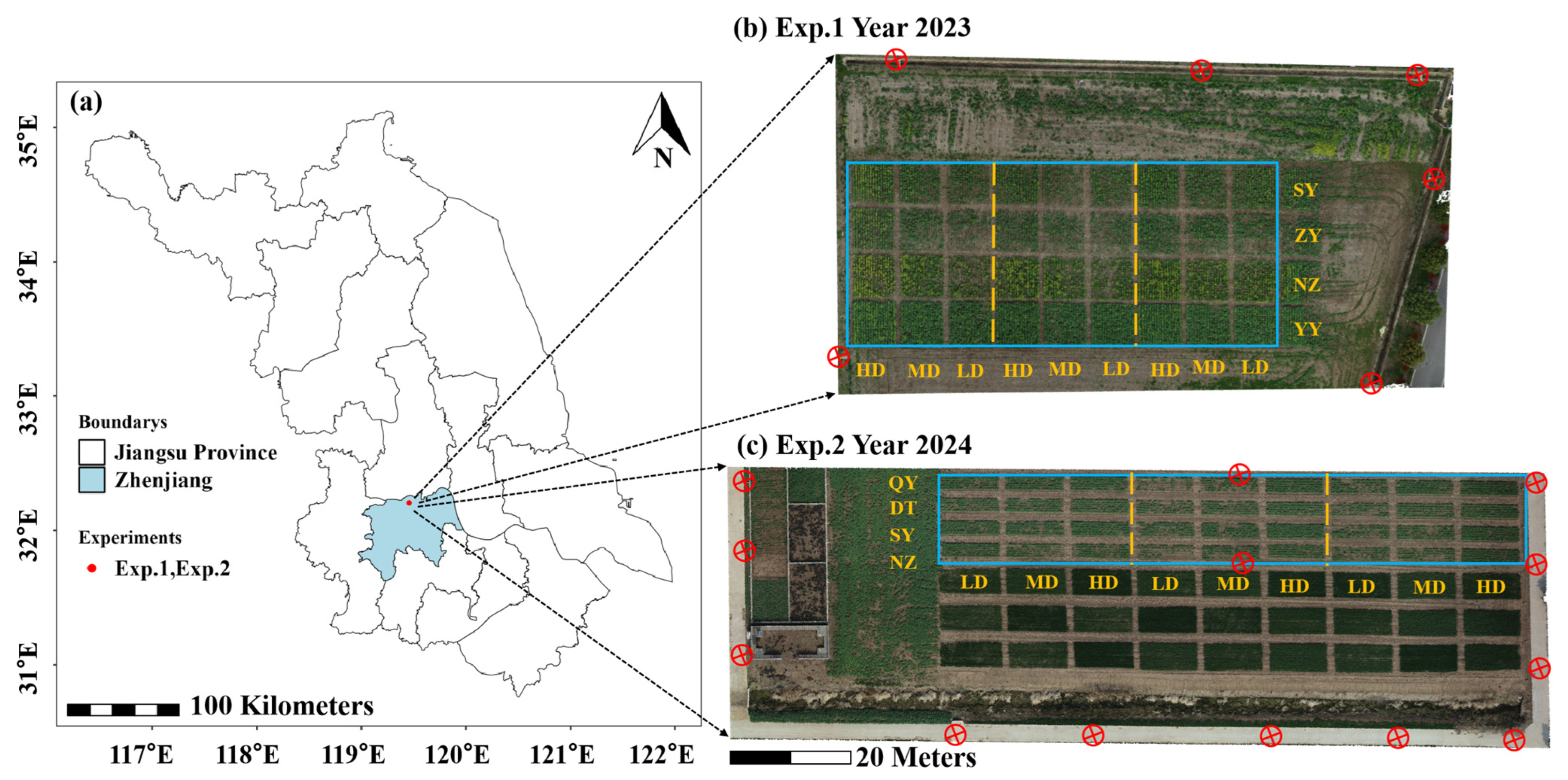
2.1. Test Site and Field Designs

The trial was carried out at the Shiyezhou Farm in Zhenjiang, Jiangsu Province, China (Figure 1). Jiangsu experiences a subtropical climate with distinct seasonal variations. In 2023, the cultivation area was divided into three replicates, each with four different rapeseed cultivars—Yangyou (YY), Suyou (SY), Ningza (NZ), and Zhongyou (ZY). Each replicate was further subdivided into three density levels: high density (0.15 m plant spacing), medium density (0.25 m plant spacing), and low density (0.35 m plant spacing). All cultivars were transplanted on 21 December 2022, with a row spacing of 0.35 m.
The cultivation area was split into three replicates for four different rapeseed cultivars—Qinyou (QY), Detian (DT), SY, and NZ—in 2024. Each replicate was also subdivided into high density (26.25 g/m2), medium density (18.75 g/m2), and low density (11.25 g/m2). Four varieties were manually sown on 17 October 2023, with rows spaced 0.35 m apart. Base fertilizer was applied at 375 kg/ha, and the irrigation method used was rain-fed.

2.2. Field Trials over Two Years

2.2.1. Field Yield Data Acquisition

On 2 June 2023, each plot was harvested and weighed separately (Figure 1). On 18 May 2024, the ‘DT 158’ was harvested manually, while other varieties were harvested on 24 May. A total of 36 valid yield data points were collected in 2023. Plots of 2 m in length were harvested and weighed. Due to disturbance during the data collection process, the rapeseed plants on the sides of the plots were omitted. Thus, the three rows of rapeseed plants were used as sampling areas. The black rectangles in Figure 1 represent these areas. The rapeseed in the sampling areas was weighed and recorded, using the measurement unit of g/m2. Because 3 plots were missing, 177 valid yield sample points were collected in 2024.
The differences resulting from the experimental treatments were assessed via a one-way analysis of variance (ANOVA) (Figure 2). The analysis showed that the density effect on rapeseed yield was non-significant. The lack of a density effect may be attributed to the compensation capacity of rapeseed. Since crops can achieve higher yields at lower seeding densities, increasing plant density above the necessary level only increases production costs without improving the yield.

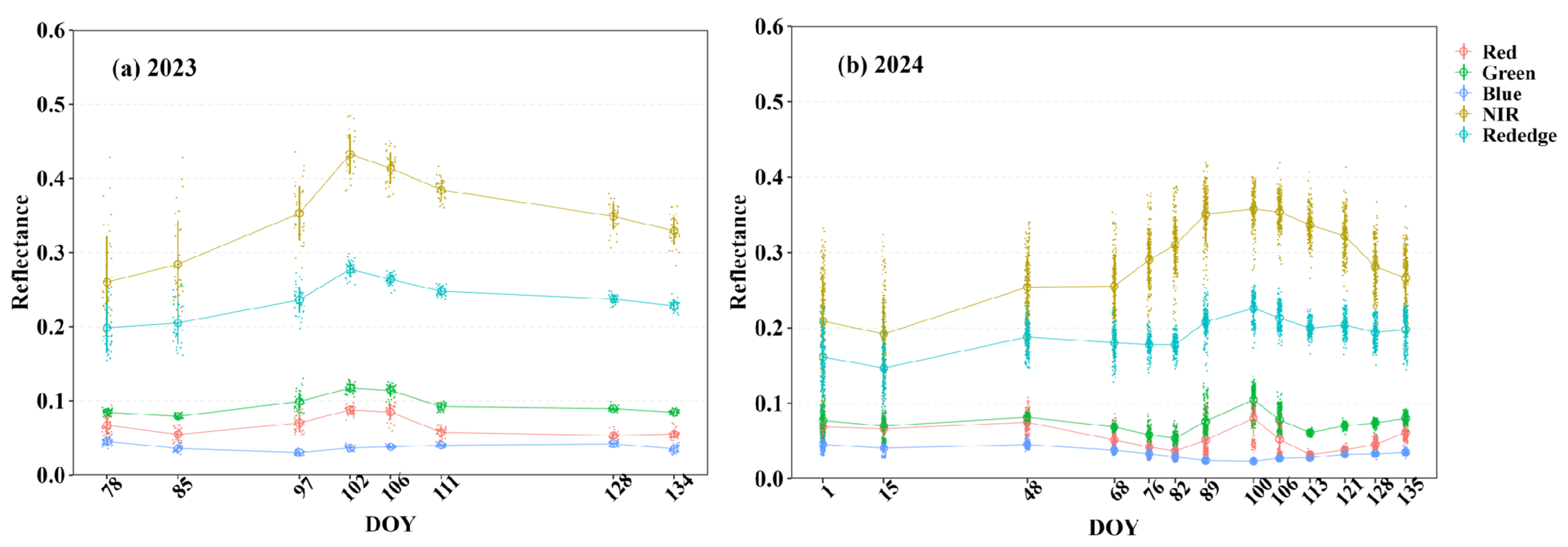
2.2.2. Multispectral Images Collection

The UAV platform offers high flexibility and enables real-time data acquisition. DJI Phantom 4 Multispectral (DJI P4M) and DJI Matrice 300 (DJI M300) equipped with L1 Camera (DJI, Shenzhen, China) were used to acquire images of rapeseed (Table 1). Although the DJI P4 includes both RGB and multispectral cameras, we chose to use the DJI M300 as it offers better pixel and spatial resolution for RGB images. The M300’s advanced features allow us to capture higher-quality images, which is essential for improving analysis accuracy and data quality. The flight mission was planned via DJI Ground Station Pro 2.0 (DJI GS pro, DJI, Shenzhen, China). Detailed geotagging of images was based on real-time kinematics (RTKs). The fine-resolution multispectral camera was fixed to a three-axis gimbal. The camera equipped in DJI P4M has a full width at half maximum of 16 nm, centered at the 450 nm, 560 nm, 600 nm, 730 nm, and 840 nm wavebands. To ensure improved consistency and accuracy in data acquisition, aerial surveys were conducted on clear, sunny days between 10:00 AM and 1:00 PM. In 2023, 8 sets of valid images were collected, covering the budding to pre-harvest. In 2024, 13 sets of valid images were collected, covering the seedling stage to pre-harvest. The flight parameters were as outlined: an altitude of 30 m, a speed of 1.5 m/s, a spatial resolution of 1.6 cm/pixel for the DJI P4M, a spatial resolution of 0.33 cm/pixel for the DJI L1, which was mounted on the DJI M300, and both forward and lateral overlaps of 85%.
In 2023, 8 sets of valid images were collected, covering the budding to pre-harvest. In 2024, 13 sets of valid images were collected, covering the seedling stage to pre-harvest. At the same time, during each aerial survey, researchers observe and record the growth stages of rapeseed, such as budding, flowering, and podding. For example, the canopy conditions during the early flowering, full flowering, and late flowering stages correspond to 10%, 50%, and 90% of the rapeseed flowers being open, respectively [31]. The podding pre-stage refers to the period after all the petals have fallen, marking the transition from flowering to the early fruiting stage in rapeseed. Table 2 presents all surveys conducted at different growth stages over the two years.
To georeference the images captured by the DJI P4M, six ground control points (GCPs) were established around the experimental plot in 2023, and thirteen GCPs were set up (Figure 1) in 2024. The exact coordinates of each GCP were measured using a Huace RTK (Shanghai Huace Navigation Technology Co., Ltd., Shanghai, China). The images of the diffuse reflector (reflectivity of 50%, size 2 m by 2 m) were collected at a height of 9.8 m. The absolute radiometric correction of the images was performed using the reflectance of the diffuse reflector. Radiometric correction converts digital numbers (DNs) into reflectance for a precise analysis of canopy spectral characteristics. A standard empirical line equation was applied to establish relationships between DNs and reflectance, using Pix4Dmapper (Pix4D SA, Lausanne, Switzerland).

2.3. Calculation and Selection of Features

2.3.1. Vegetation Index

This study employed Pix4Dmapper 4.4.12 to calibrate and stitch multispectral images captured by a UAV (Pix4D, Lausanne, Switzerland). Using the coordinates of the sampling grid, regions of interest (ROI) for each yield sampling point were generated in ENVI 5.3.1 software (Exelis Visual Information Solutions, Boulder, CO, USA). Then, the average values of the 5 spectral reflectances provided by the DJI P4M within the ROI were extracted. Figure 3 exhibits the spectral reflectance of all valid images for 2023 and 2024. The VIs were calculated by averaging the VIs of all pixels within the ROI. Eight VIs commonly used to estimate chlorophyll, LAI, or yield were selected for analyzing their correlation with rice grain yield (Table 3). For example, CIre was commonly used to indicate the LAI of complex canopies and has been validated as an effective indicator for rapeseed yield prediction (Peng et al., 2019 [16]). Alternatively, the NDVI was commonly employed for yield estimation prior to flowering (Dong et al., 2019 [14]).

2.3.2. Texture Features

The Gray Level Co-occurrence Matrix (GLCM) algorithm was employed to extract 8 TFs (Mean, Var, Hom, Con, Dis, Ent, 2nd_m and Cor) from the RGB images. These variables represent the spatial connection between two pixels [39]. The GLCM was calculated with motion directions (1, 1) within 3 × 3 windows, and the mean value was considered as the final texture feature. The texture analysis generated 8 variables for each band (Red, Green, Blue). Texture features were labeled by combining the band abbreviation with the texture name. For example, ‘Mean_r’ refers to the ‘Mean’ feature at the red band. In 2023, there are 13 dates for TFs, and a total of 312 (13 × 3 × 8) texture feature datasets were established. In 2024, there are 17 dates, and a total of 408 (17 × 3 × 8) texture feature datasets were set up.

2.4. Regression Models

ML algorithms, like partial least squares regression (PLSR), support vector regression (SVR), and RFs were used for yield prediction. The dataset is randomly split into 86% for training (152) and 14% for testing (25). To eliminate the uncertainty of the coefficient of determination (R2) caused by data splitting, we performed 7-fold cross-validation. The model was assessed using evaluation criteria such as RMSE (root mean squared error), rRMSE (relative root mean square error), and R2.
R 2 = 1 i = 1 n ( y i y ^ i ) / i = 1 n ( y i y ¯ i )
R M S E = 1 / n i = 1 n ( y i y ^ i )
r R M S E = ( R M S E / y ¯ ) × 100 %
where y i and y i denote the observed and simulated rapeseed yield, respectively. y ¯ i denotes the mean of observed rapeseed yield, and n is the total samples size in the training set.

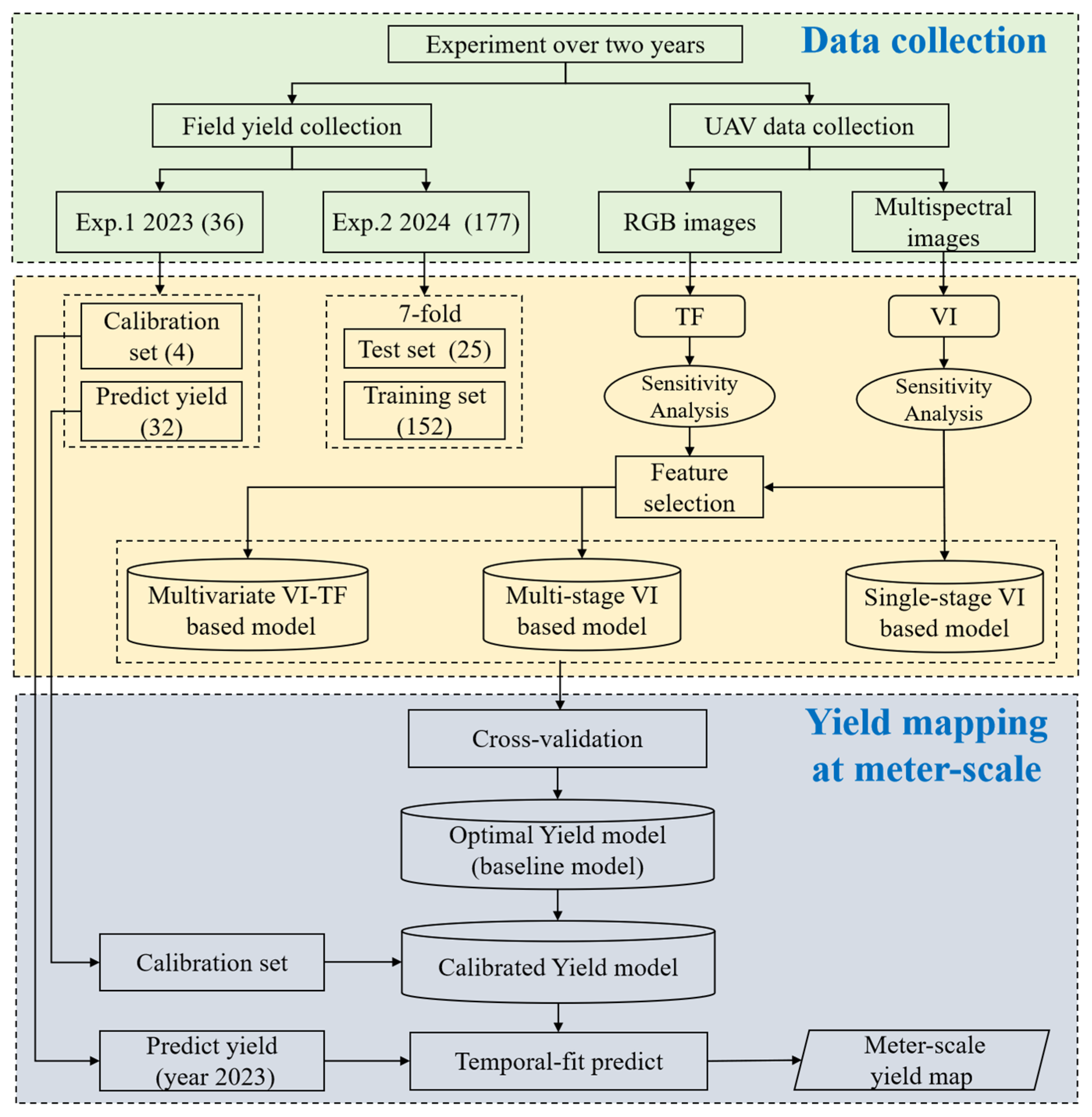
2.5. Yield Prediction Framework

The flowchart of the modeling process for rapeseed yield prediction consists of four stages: image acquisition and data collection, feature selection and modeling, model calibration and validation, and yield map generation (Figure 4). First, image acquisition; data collection; feature extraction; and the RF, SVR, and PLSR models have been introduced in Section 2.2, Section 2.3 and Section 2.4. Second, the sensitivity analysis of VIs, TFs, and rapeseed yield at different growth stages was conducted using the Pearson correlation coefficient. Feature selection was performed using VIP scores, followed by the evaluation of their contributions to machine learning models through Shapley additive explanations (SHAP).
Next, the features and ML models selected based on the cross-validated RMSE are defined as the baseline model for rapeseed yield prediction. Based on the actual measured data (Figure 2), the distributions of rapeseed yield were different among the four varieties. Therefore, this study selected data from four different varieties in 2023 to calibrate the model by fine-tuning the hyper-parameters (Figure 5). The yield data from each plot in 2023 were aggregated, and yield classes were assigned based on predefined thresholds. Points above the 90% were categorized as ‘high yield’, while those below the 10% were labeled ‘low yield’. The remaining range was divided into three equal parts, designated as ‘medium-high yield’, ‘medium yield’, and ‘medium-low yield’.
Finally, the spatial distribution map of rapeseed yield was generated. Specifically, this process was carried out in three key steps: (1) the images were rotated according to the different planting orientations in 2023 and 2024 (65.7° for 2023 and 24.3° for 2024); (2) reflectance values of the meter-scale pixels were extracted based on the spatial resolution of the images; and (3) the yield distribution maps generated by the proposed model were visualized.

2.6. Software

All statistical analyses were carried out in R software (version 4.3.3). For ANOVA, tests were performed using the ‘Stats’ package (part of R basics). All TFs were extracted using the ‘GLCM’ (version 1.6.5) package. RF, PLSR, and SVR were developed using the ‘randomForest’ (version 4.7.1.1), ‘pls’ (version 2.8.3), and ‘e1071’ (version 1.7.14) packages. Pearson correlations were used from the ‘Corrplot’ library (version 0.92); VIP sores for each feature were extracted using the ‘importance’ function from the ‘randomForest’ package; the contribution of variables to ML models was determined based on the Shapley value concept from game theory, and was implemented using the ‘Shapley$new’ function from the ‘iml’ package (version 0.11.4); and data manipulation was carried out using ‘dplyr’ (version 1.1.4) and ‘tidyr’ (version 1.3.1) packages. Detailed information about these packages can be found on CRAN: https://cran.r-project.org/.

3. Results

3.1. Sensitivity Analysis of Model Features

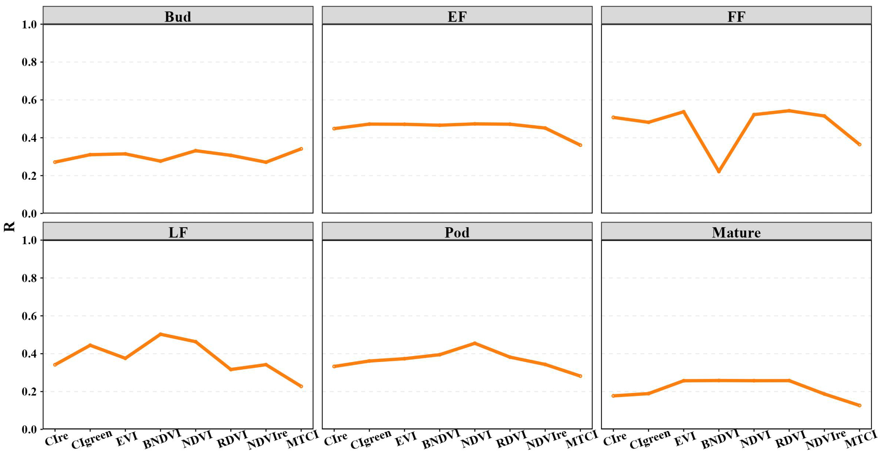
3.1.1. Relationship Between VIs at Single-Stage and Rapeseed Yield

As shown in Figure 6, the Pearson correlation coefficients between VIs and rapeseed yield at various growth phases are represented by each line, derived from 108 samples (36 plots × 5 sampling locations in 2024). Overall, the R value between VIs and rapeseed yield estimation increased from the budding stage, peaked at full flowering, and subsequently decreased at the maturing stage. Additionally, data analysis reveals that the correlation between the VIs and yield in 2024 is moderate. This pattern may be due to the fact that as the sample size increases, the correlation between VIs and rapeseed yield becomes more influenced by environmental conditions, thus lowering the R value.

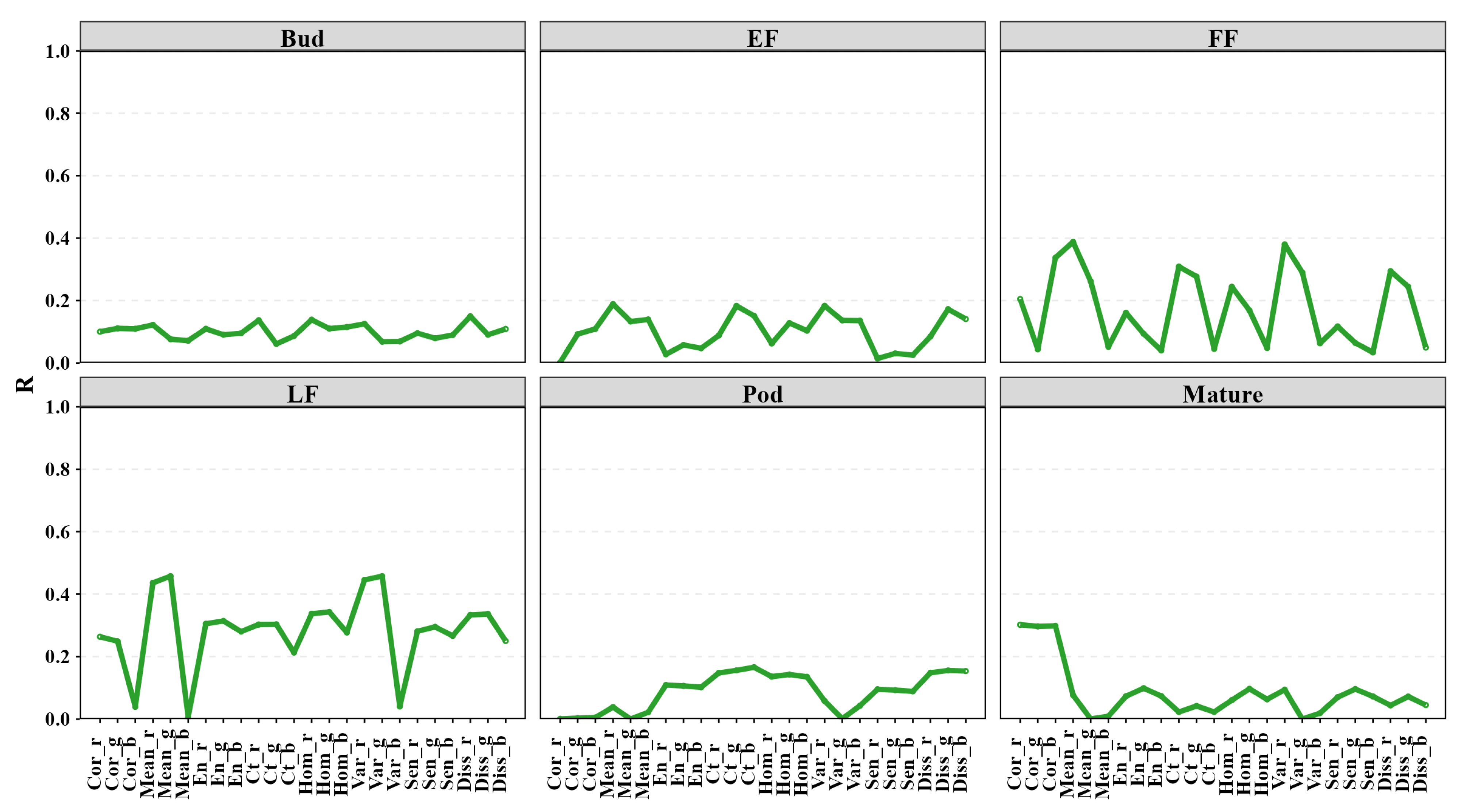
3.1.2. Relationship Between TFs at Single-Stage and Rapeseed Yield

First, the relationship between TFs and rapeseed yield over the entire growth period was analyzed using the Pearson correlation coefficient. Compared to the performance of VIs (Figure 6), the R value between TFs and rapeseed yield was higher at the budding and maturing stages (Figure 7). A strong correlation was found between Mean_g, En_g, and rapeseed yield at various stages. The relationship between TFs and rapeseed yield at different growth phases was inconsistent.

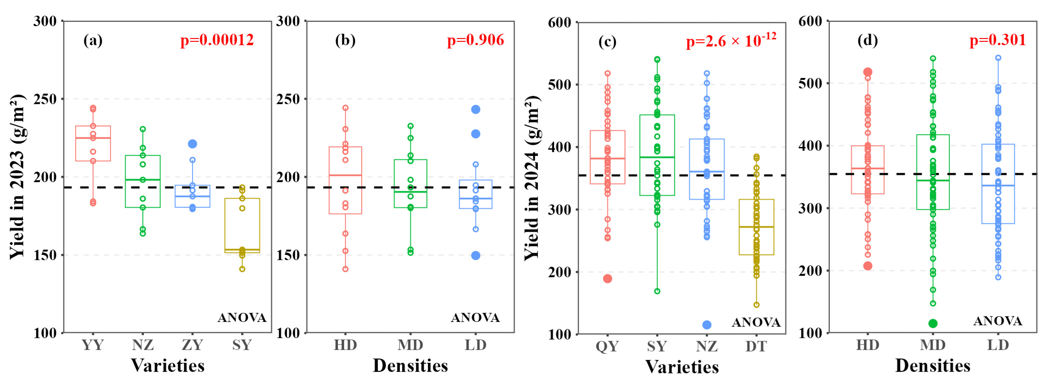
3.2. Results of Yield Prediction in 2024

3.2.1. Single-Stage Prediction

Table 4 presents the yield prediction performance of the RF, SVR, and PLSR models using seven VIs at four individual growth stages, as described in Section 2.3.1. RF, SVR, and PLSR models achieved the highest accuracy in predicting rapeseed yield during the late flowering stages. The RF model performed well on the training data, with an R2 of 0.91 and an rRMSE of 8.47%, but showed poor results on the test dataset, with an R2 of 0.40 and an rRMSE of 19.06%, indicating overfitting. All single-stage VI-based models exhibited poor performance on the test dataset, indicating limited stability.

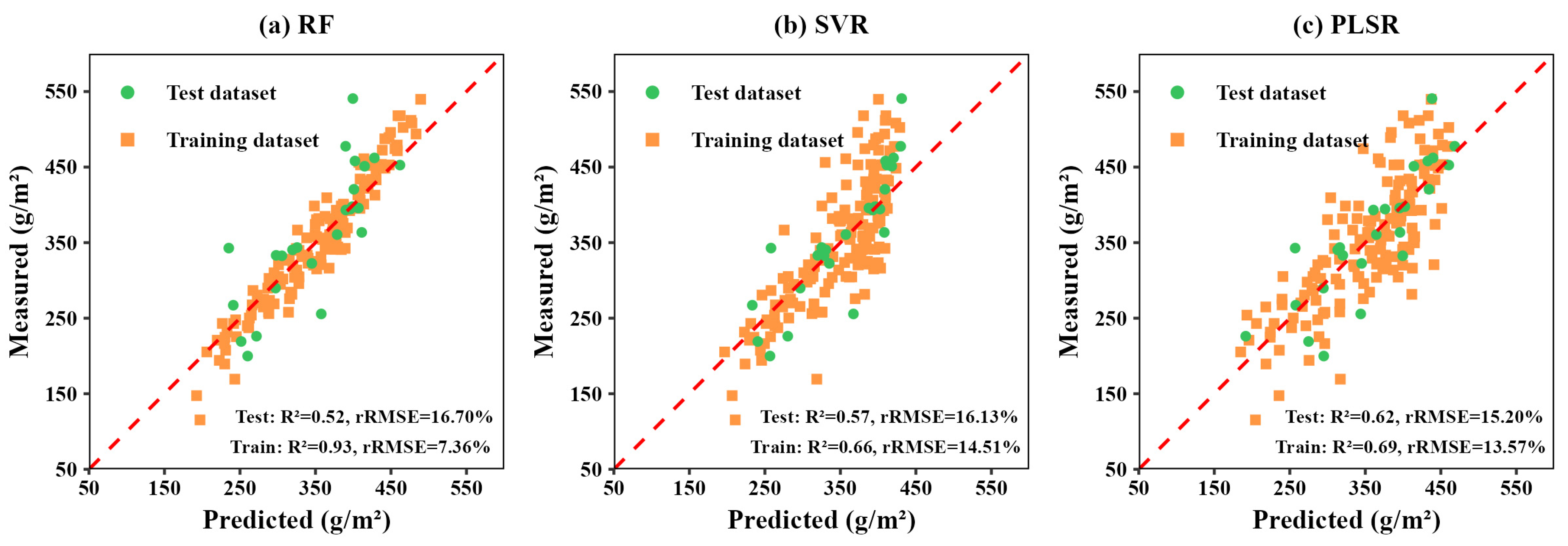
3.2.2. Multi-Stage Prediction

When multi-stage spectral VIs are used for rapeseed yield estimation, they enable the exploration of effective spectral information from key growth stages associated with rapeseed yield, aiming to improve the model’s generality. Additionally, this study explored the potential of models that integrate VIs and TFs for rapeseed yield estimation. As shown in Figure 8, the VIP score derived from the RF regression model provided the foundation for selecting key phenological stages and model input variables. Compared to the single-stage VIs, all models exhibited more robust performance with the multi-stage VI-based yield prediction model (Table 5). Figure 9 shows the scatter plots for the models based on multi-stage VIs. The best rRMSE results for the RF, SVR, and PLSR models were 16.70%, 16.13%, and 15.20%, respectively, and the corresponding R2 values were 0.52, 0.57, and 0.62. Results also showed that the PLSR model was superior to the RF and SVR models on the test dataset. However, the multi-stage multivariate VI-TF did not effectively improve the robustness and accuracy for the rapeseed yield prediction.
To further enhance the model’s interpretability and transparency, this study employed SHAP to investigate the contributions of spectral and TFs to the model’s yield estimation (Figure 10). Results showed that, in rapeseed yield models, spectral variables had a greater contribution than texture variables. The correlation between TFs and rapeseed yield is weak, and incorporating these features into the model may increase its complexity without yielding any improvement in predictive accuracy. We further refined the analysis of the contributions of spectral features at different stages to rapeseed yield estimation. Results showed that spectral indices during the full flowering and late flowering stages proved to be the most effective variables for estimating rapeseed yield. By combining the features selected through VIP with SHAP analysis, the multi-stage VIs, from the budding to podding stage, were better able to capture variations in rapeseed yield. This approach not only enhances the precision of models but also identifies the most appropriate stage for rapeseed yield predictions.

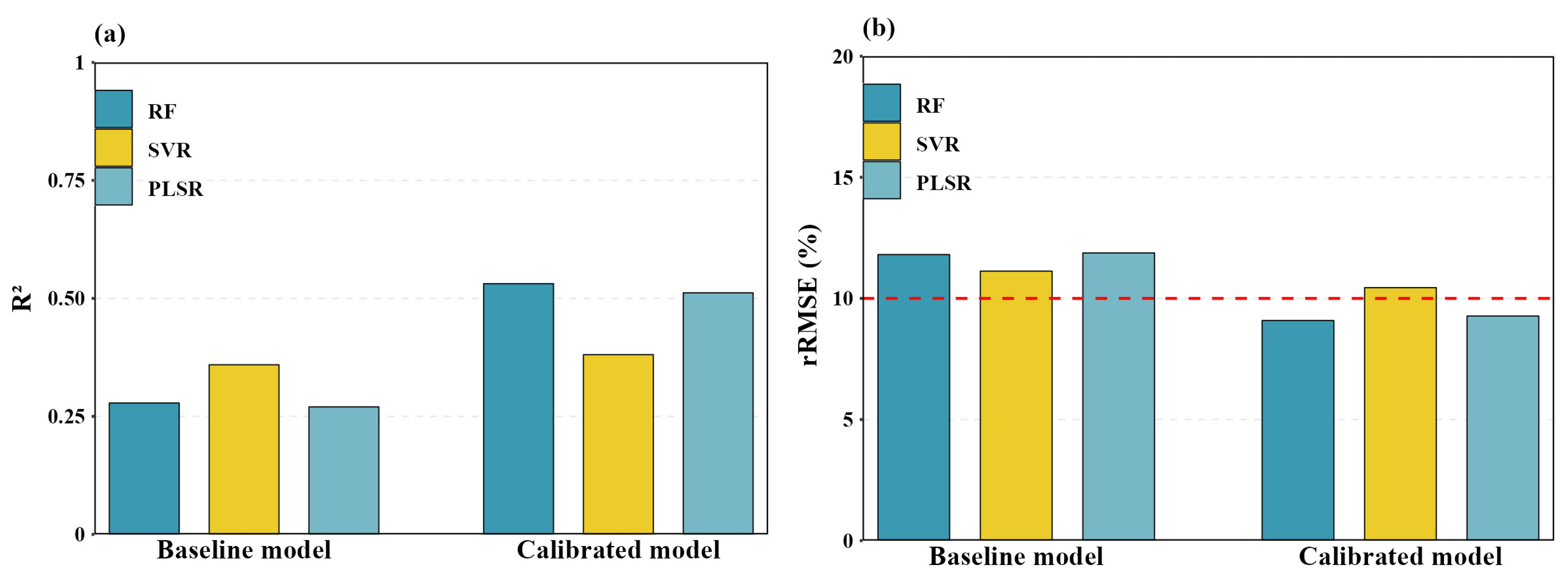
3.3. Validation Results of Yield Prediction of Temporal-Fit Scenario

As illustrated in Figure 11, the baseline model exhibited relatively poor performance in cross-year rapeseed yield prediction, whereas the calibrated models demonstrated significant improvement in accuracy. The results suggested that the transfer of knowledge gained in 2023 greatly enhances the model’s generality to predict yields across different years. Tuning the internal parameters makes the model more suitable for complex production environments, enabling accurate rapeseed yield prediction. The findings suggest that the fine-tuned RF model attained the highest precision in the temporal fit (R2 = 0.53, rRMSE = 9.09%). In contrast to the baseline RF model, the updated RF model increased R2 by 25% and reduced the rRMSE below 10%. The updated SVR model yielded a minimal improvement in rapeseed yield prediction accuracy. One possible reason is that updating the SVR model requires manual optimization, and the potential for improvement through transfer learning is limited.
As shown in Figure 12, The yield class maps obtained from the calibrated RF model were comparable to those generated with the rapeseed yield data. However, the accuracy was lower in certain field plots, likely due to the insufficient number of training samples for each yield class. Since harvesters typically adjust their speed in real time based on field yield, yield class maps that align with actual planting patterns provide valuable guidance for optimizing harvester speed control.

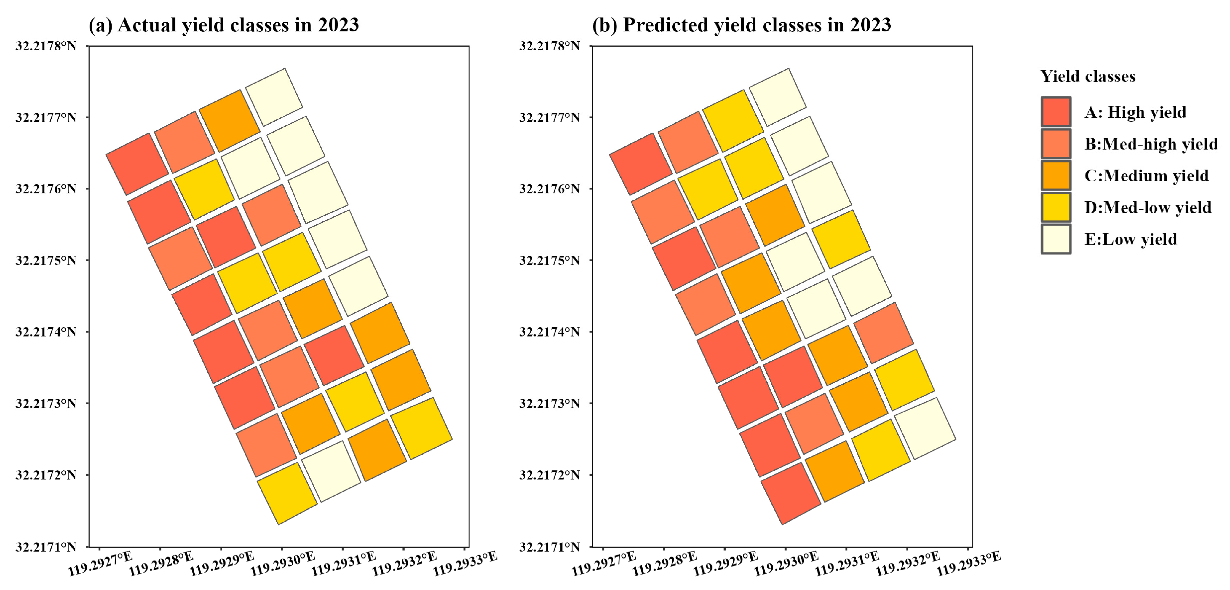
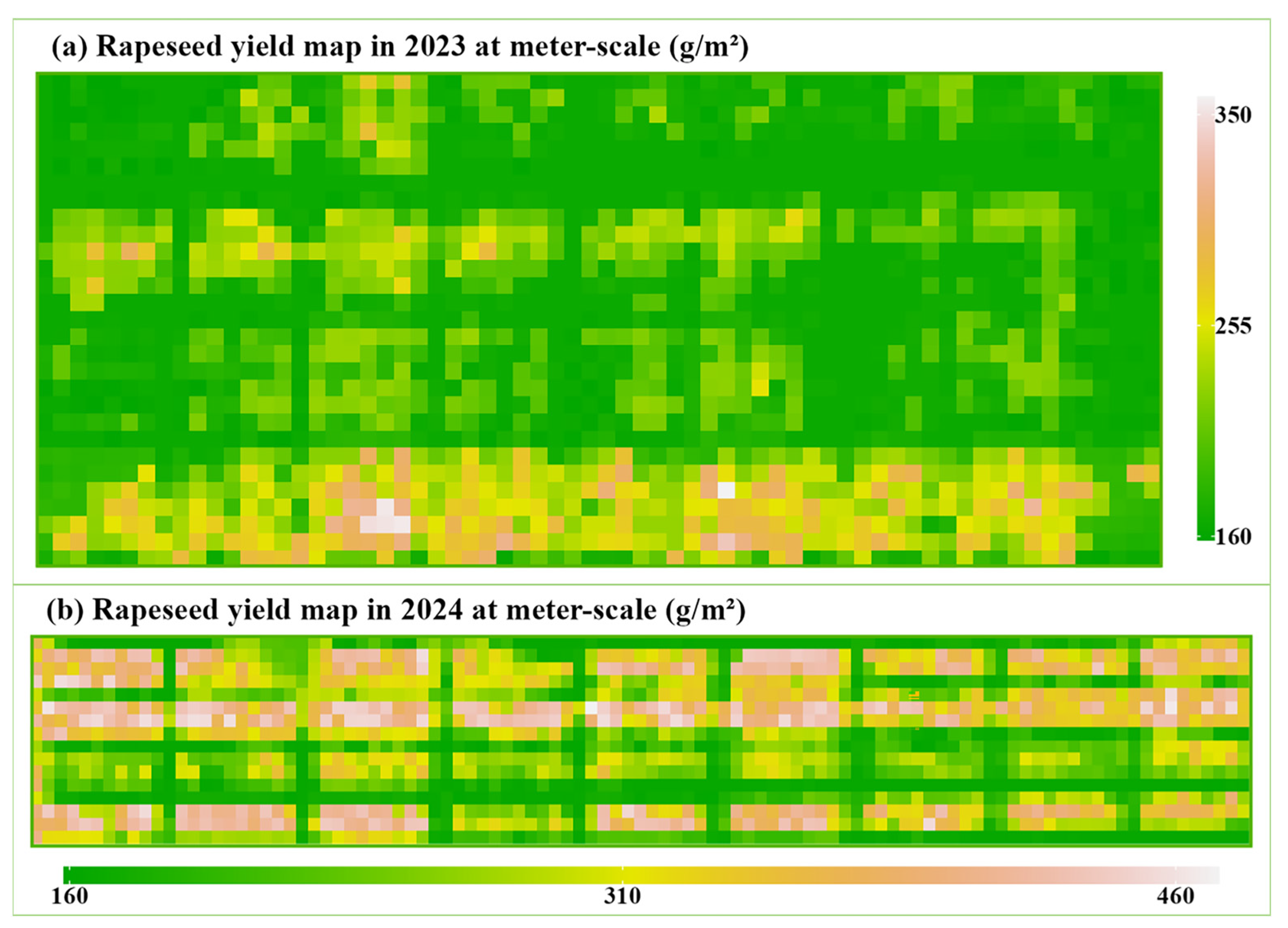
3.4. Yield Distribution Map at Meter-Scale

To further compare the spatial distribution of rapeseed yield estimated, we generated the meter-scale yield maps using multi-stage VIs and transferred RF model (Figure 13). Both yield distributions were clearly related to the varieties. YY had a higher yield at 2023, and DT had a lower yield at 2024. In comparison, the response of the density levels to rapeseed yield was notable only in some plots. Accurate yield distribution maps at meter-scale enable more precise control of harvesting parameters, thereby promoting the advancement of precision agriculture. Before harvest, obtaining accurate meter-scale yield distribution maps provides the foundation for controlling the forward speed and cutter bar height of smart harvesters. This helps ensure a stable feed rate, thereby reducing harvest losses caused by unstable input rates. The accuracy and timeliness of this information are critical for optimizing the operation of smart harvesters and enhancing overall harvesting efficiency.

4. Discussion

4.1. Contrasting Multi-Stage and Multivariate Models

This study utilized VIs and TFs as inputs within the ML framework for rapeseed yield prediction. The superior performance of the multi-stage models, compared to the single-stage models, indicates that the multi-stage features effectively capture the spectral information of the rapeseed canopy at different phases of development. The property of multi-feature fusion in estimating rapeseed yield was studied in this research. A multi-stage VI model and a multivariate VI-TF model were developed using the top variables selected according to VIP scores. Our results indicated that models employing multi-stage VIs performed better than those employing multi-stage VI-TFs (Table 5). In most cases, multiple feature combinations provided a model that estimated yields closer to the measured values [40,41]. However, our study found that the fusing TFs did not effectively improve the robustness of the model. One possible explanation is that the high-dimensional TFs capture microscopic details of the canopy surface; however, these structural details may have a weak correlation with rapeseed yield, resulting in a minimal contribution of texture features to the yield prediction model.
This study evaluated the performance of PLSR and RF regression models using various data fusion approaches combining texture and spectral features. In the case of the models, the PLSR model showed good performance. Specifically, when using multi-stage VIs from the flowering to podding stage, the yield prediction error was 15.20%, and the R2 value reached 0.62. The RF model exhibited high accuracy in the training set but performed moderately in the test set, indicating overfitting. However, the RF had strong model transfer-learning capabilities, achieving optimal performance in temporal-fit tests. While conventional regression methods may suffice, ensemble learning techniques such as RF offer greater precision and reliability in complex, multi-year scenarios.
Additionally, this study identified the most appropriate phenological window for rapeseed yield prediction, spanning from the budding to the podding stage. Similarly, studies have found that the budding and flowering stages represent the most informative period for acquiring imagery for rapeseed yield modeling [15,16]. However, this study found that the spectral information during the pod filling stage also provides crucial information for the rapeseed yield model, as the number and quality of pods directly influence the yield potential. By focusing the modeling process on multiple key phenological stages, we were able to eliminate redundant data, ultimately enhancing the accuracy of the rapeseed yield prediction model. Our findings show that defining time windows based on growth stages is an effective approach to account for the varying environmental impacts on rapeseed at different stages. Factoring in stage data offers a holistic understanding of the environment’s impact on yield, ultimately leading to refined prediction capabilities and improved model accuracy.

4.2. Yield Prediction Performance at Temporal-Fit Scenario

Our results highlight the potential to extend rapeseed yield prediction over two years by training with a limited number of yield monitor data plots. In this study, we calibrated ML models using yield data from four varieties, which enhanced the model’s generality for predicting yields in unknown years. Temporal variations introduce domain shifts in remote sensing data. Planting methods and climate conditions differed between years. In 2023, the experimental area experienced a cold winter, resulting in frost damage to the rapeseed. As a result, plant height in 2023 was significantly lower than in 2024, by nearly 50 cm. Additionally, sowing methods varied between the two years: transplanting was used in 2023 at a lower density, while broadcasting was employed in 2024 at a higher density.
Differences in growth patterns, yield potential, and responses to environmental conditions among rapeseed varieties can cause variation in yield data (Figure 2). By using data from multiple varieties to calibrate the model, it can better handle this variation and improve predictions under different environmental conditions and years. This calibration enables the model to better account for key factors influencing yield, such as variations in soil conditions, climate, and agricultural management practices, which can change annually. By incorporating this variability, the model is better able to generalize to new planting seasons, thereby enhancing the accuracy of cross-year yield predictions. Additionally, the annual fitting method benefits from transfer learning. The model is first trained on data from one year and then used to predict the yield for another year. This approach improves prediction accuracy by applying knowledge gained from the year before, reducing data collection costs.
Furthermore, selecting appropriate plots, with representative yield categories, is crucial for reliable cross-year yield prediction. The actual yield map and the predicted yield map displayed similar distributions, though some differences were observed in certain plots (Figure 12). The accuracy of rapeseed yield prediction may be influenced by the quantity of available training data. Sunoj found that training data should consist of at least 20% from each yield category to enable yield prediction for a future year [42]. Thus, using data from more fields and incorporating data with varying yield variability to train the model may further improve the accuracy of yield predictions across different years. Additionally, extending the time frame allows the model to learn from variations in weather, soil conditions, and rainfall across different years, leading to more accurate yield predictions.

4.3. Application Potential and Limitations

Accurately predicting rapeseed yield in advance is highly beneficial for precision agriculture and harvesting decision-making. Our results highlighted the effectiveness of multi-stage VIs in estimating rapeseed yield, outperforming all validation datasets. However, VIs are prone to spectral saturation, which may prevent them from capturing key factors that influence yield. Future research could explore more comprehensive feature fusion and the application of different sensing technologies. First, the inclusion of additional feature datasets should be explored, such as fertilizer application and soil moisture. Second, the integration of available high spatial resolution satellites to obtain meter-scale remote sensing information should be explored to enable yield prediction across multiple regions.
Alternatively, we highlight the benefits of a calibrated RF model in temporal-fit rapeseed yield prediction. The collection of such training data is expensive, particularly for agricultural fields that require labor-intensive fieldwork and destructive sampling methods. By updating RF model parameters, the model can achieve more accurate yield estimation with smaller samples. Our results show that rapeseed yield predictions can be extended to the entire farm by training with data from different varieties. Therefore, the proposed method holds potential for pre-harvest rapeseed yield prediction in practice.
Nevertheless, this study has limitations that future research should address. Consistency in farm management practices, including irrigation, fertilization, and the uniformity of planting areas and varieties, could further enhance the accuracy of yield predictions. Additionally, efforts will focus on enhancing the model’s temporal accuracy, including data precision, temporal consistency. Further research will also explore the model’s application and the development of a management system for rapeseed harvesting decisions. The modeling technology could eventually be integrated into smart harvesters to improve rapeseed yield and quality, as well as support the adoption of these systems.

5. Conclusions

This paper evaluated the applicability of single-stage VIs, multi-stage VIs, and multivariate VI-TFs for rapeseed yield prediction. We also explored the advantages of the transferred model for rapeseed yield prediction over multiple years. Results demonstrated that multi-stage VIs outperformed single-stage VIs. The multivariate VI-TFs model did not improve the robustness of yield prediction. Our study also found that a period of approximately one to two months before harvest is an ideal lead time for rapeseed yield prediction. Additionally, in the temporal-fit scenario, calibrating the RF model with yield data from different varieties significantly improved the accuracy of cross-year yield predictions. Compared to the baseline RF model, the calibrated RF model increased R2 by 25% and reduced the rRMSE to below 10%. The findings highlight the potential of multi-stage VIs from the flowering to podding stage, as well as the calibrated RF model, for multi-year rapeseed yield prediction. This study provides data and technical support for the promotion of smart harvesters at the farm scale.

Author Contributions

Y.Z.: writing—original draft, investigation, methodology, software, conceptualization, writing— review and editing; Z.C.: software; X.C.: investigation; Y.N.: writing—review and editing, investigation, supervision, funding acquisition; L.X.: writing—review and editing, supervision, funding acquisition. All authors have read and agreed to the published version of the manuscript.

Funding

This work was funded by the National Key R&D Program Projects during the 14th Five-Year Plan [grant number 2023YFD2001003]; the National Natural Science Foundation of China [grant number 32401695]; the Science and Technology Major Project of Anhui Province [grant number 202203a06020025]; the China Agriculture Research System of MOF and MARA CARS-12; the Natural Science Foundation of Jiangsu Province [grant number BK20240878]; and the China Postdoctoral Science Foundation [grant number 2024M751186].

Data Availability Statement

The raw data supporting the conclusions of this article will be made available by the authors upon request.

Acknowledgments

We warmly thank the staff of the Shiyezhou Farm, without whom the two-year field experiments and this research would not have been possible. We also thank Moran Zhuang of DJI for support with the UAV operations.

Conflicts of Interest

The authors declare that they have no known competing financial interests or personal relationships.

References

  1. Velde, M.; Bouraoui, F.; Aloe, A. Pan-European regional-scale modelling of water and N efficiencies of rapeseed cultivation for biodiesel production. Glob. Change Biol. 2008, 15, 24–37. [Google Scholar] [CrossRef]
  2. Nowosad, K.; Liersch, A.; Popławska, W.; Bocianowski, J. Genotype by environment interaction for seed yield in rapeseed (Brassica napus L.) using additive main effects and multiplicative interaction model. Euphytica 2015, 208, 187–194. [Google Scholar] [CrossRef]
  3. Kirkegaard, J.A.; Lilley, J.M.; Brill, R.D.; Ware, A.H.; Walela, C.K. The critical period for yield and quality determination in canola (Brassica napus L.). Field Crops Res. 2018, 222, 180–188. [Google Scholar] [CrossRef]
  4. Wan, L.; Liu, Y.; He, Y.; Cen, H. Prior knowledge and active learning enable hybrid method for estimating leaf chlorophyll content from multi-scale canopy reflectance. Comput. Electron. Agric. 2023, 214, 106485. [Google Scholar] [CrossRef]
  5. Zhao, Y.; Meng, Y.; Han, S.; Feng, H.; Yang, G.; Li, Z. Should phenological information be applied to predict agronomic traits across growth stages of winter wheat? Crop J. 2022, 10, 1346–1352. [Google Scholar] [CrossRef]
  6. Lu, X.; Shen, Y.; Xie, J.; Yang, X.; Shu, Q.; Chen, S.; Shen, Z.; Cen, H. Phenotyping of Panicle Number and Shape in Rice Breeding Materials Based on Unmanned Aerial Vehicle Imagery. Plant Phenomics 2024, 6, 0265. [Google Scholar] [CrossRef]
  7. Malambo, L.; Popescu, S.C.; Murray, S.C.; Putman, E.; Pugh, N.A.; Horne, D.W.; Richardson, G.; Sheridan, R.; Rooney, W.L.; Avant, R.; et al. Multitemporal field-based plant height estimation using 3D point clouds generated from small unmanned aerial systems high-resolution imagery. Int. J. Appl. Earth Obs. Geoinf. 2018, 64, 31–42. [Google Scholar] [CrossRef]
  8. Lin, Y.C. Ayman. Quality control and crop characterization framework for multi-temporal UAV LiDAR data over mechanized agricultural fields. Remote Sens. Environ. 2021, 256, 112307. [Google Scholar] [CrossRef]
  9. Teshome, F.T.; Bayabil, H.K.; Hoogenboom, G.; Schaffer, B.; Singh, A.; Ampatzidis, Y. Unmanned aerial vehicle (UAV) imaging and machine learning applications for plant phenotyping. Comput. Electron. Agric. 2023, 212, 108064. [Google Scholar] [CrossRef]
  10. Gu, Q.; Huang, F.; Lou, W.; Zhu, Y.; Hu, H.; Zhao, Y.; Zhou, H.; Zhang, X. Unmanned aerial vehicle-based assessment of rice leaf chlorophyll content dynamics across genotypes. Comput. Electron. Agric. 2024, 221, 108821. [Google Scholar] [CrossRef]
  11. Zhang, M.; Gao, Y.; Zhang, Y.; Fischer, T.; Zhao, Z.; Zhou, X.; Wang, Z.; Wang, E. The contribution of spike photosynthesis to wheat yield needs to be considered in process-based crop models. Field Crops Res. 2020, 257, 107931. [Google Scholar] [CrossRef]
  12. Li, H.; Zhao, C.; Yang, G.; Feng, H. Variations in crop variables within wheat canopies and responses of canopy spectral characteristics and derived vegetation indices to different vertical leaf layers and spikes. Remote Sens. Environ. 2015, 169, 358–374. [Google Scholar] [CrossRef]
  13. Sulik, J.J.; Long, D.S. Spectral indices for yellow canola flowers. Int. J. Remote Sens. 2015, 36, 2751–2765. [Google Scholar] [CrossRef]
  14. Dong, T.; Shang, J.; Qian, J.; Ma, B.; Kovacs, B.; Walters, J.M.; Jiao, D.; Geng, X.; Shi, X.; Cheng, Y. Assessment of red-edge vegetation indices for crop leaf area index estimation. Remote Sens. Environ. 2019, 222, 90–102. [Google Scholar] [CrossRef]
  15. Sulik, J.J.; Long, D.S. Spectral considerations for modeling yield of canola. Remote Sens. Environ. 2016, 184, 161–174. [Google Scholar] [CrossRef]
  16. Peng, Y.; Zhu, T.E.; Li, Y.; Dai, C.; Fang, S.; Gong, Y.; Wu, X.; Zhu, R.; Liu, K. Remote prediction of yield based on LAI estimation in oilseed rape under different planting methods and nitrogen fertilizer applications. Agric. For. Meteorol. 2019, 271, 116–125. [Google Scholar] [CrossRef]
  17. Fan, H.; Liu, S.; Li, J.; Li, L.; Dang, L.; Ren, T.; Lu, J. Early prediction of the seed yield in winter oilseed rape based on the near-infrared reflectance of vegetation (NIRv). Comput. Electron. Agric. 2021, 186, 106314. [Google Scholar] [CrossRef]
  18. Duan, B.; Fang, S.; Gong, Y.; Peng, Y.; Wu, X.; Zhu, R. Remote estimation of grain yield based on UAV data in different rice cultivars under contrasting climatic zones. Field Crops Res. 2021, 267, 108148. [Google Scholar] [CrossRef]
  19. Lu, L.; Luo, J.; Xin, Y.; Duan, H.; Sun, Z.; Qiu, Y.; Xiao, Q. How can UAV contribute in satellite-based Phragmites australis aboveground biomass estimating? Int. J. Appl. Earth Obs. Geoinf. 2022, 114, 102712. [Google Scholar] [CrossRef]
  20. Zhou, X.; Zheng, H.B.; Xu, X.Q.; He, J.Y.; Ge, X.K.; Yao, X.; Cheng, T.; Zhu, Y.; Cao, W.; Tian, Y. Predicting grain yield in rice using multi-temporal vegetation indices from UAV-based multispectral and digital imagery. ISPRS J. Photogramm. Remote Sens. 2017, 130, 246–255. [Google Scholar] [CrossRef]
  21. Navarro, A.; Young, M.; Allan, B.; Carnell, P.; Macreadie, P.; Ierodiaconou, D. The application of unmanned aerial vehicles (UAVs) to estimate above-ground biomass of mangrove ecosystems. Remote Sens. Environ. 2020, 242, 111741. [Google Scholar] [CrossRef]
  22. Du, R.; Lu, J.; Xiang, Y.; Zhang, F.; Chen, J.; Tang, Z.; Shi, H.; Wang, X.; Li, W. Estimation of winter canola growth parameter from UAV multi-angular spectral-texture information using stacking-based ensemble learning model. Comput. Electron. Agric. 2024, 222, 109074. [Google Scholar] [CrossRef]
  23. Ji, Y.; Liu, Z.; Liu, R.; Wang, Z.; Zong, X.; Yang, T. High-throughput phenotypic traits estimation of faba bean based on machine learning and drone-based multimodal data. Comput. Electron. Agric. 2024, 227, 109584. [Google Scholar] [CrossRef]
  24. Mateo-Sanchis, A.; Piles, M.; Muñoz-Marí, J.; Adsuara, J.E.; Pérez-Suay, A.; Camps-Valls, G. Synergistic integration of optical and microwave satellite data for crop yield estimation. Remote Sens. Environ. 2019, 234, 111391. [Google Scholar] [CrossRef]
  25. van Klompenburg, T.; Kassahun, A.; Catal, C. Crop yield prediction using machine learning: A systematic literature review. Comput. Electron. Agric. 2020, 177, 105735. [Google Scholar] [CrossRef]
  26. Li, Z.; Zhao, Y.; Taylor, J.; Gaulton, R.; Jin, X.; Song, X.; Li, Z.; Meng, Y.; Chen, P.; Feng, H.; et al. Comparison and transferability of thermal, temporal and phenological-based in-season predictions of above-ground biomass in wheat crops from proximal crop reflectance data. Remote Sens. Environ. 2022, 273, 112133. [Google Scholar] [CrossRef]
  27. Louzada Pereira, L.; Carvalho Guarçoni, R.; Soares Cardoso, W.; Côrrea Taques, R.; Rizzo Moreira, T.; da Silva, S.F.; Schwengber ten Caten, C. Influence of Solar Radiation and Wet Processing on the Final Quality of Arabica Coffee. J. Food Qual. 2018, 2018, 6408571. [Google Scholar] [CrossRef]
  28. Michau, G.; Fink, O. Unsupervised transfer learning for anomaly detection: Application to complementary operating condition transfer. Knowl.-Based Syst. 2021, 216, 106895. [Google Scholar] [CrossRef]
  29. Meiyan, S.; Mengyuan, S.; Qizhou, D.; Xiaohong, Y.; Baoguo, L.; Yuntao, M. Estimating the maize above-ground biomass by constructing the tridimensional concept model based on UAV-based digital and multi-spectral images. Field Crops Res. 2022, 282, 107472. [Google Scholar] [CrossRef]
  30. Ye, Y.; Jin, L.; Bian, C.; Xian, G.; Lin, Y.; Liu, J.; Guo, H. Estimating potato aboveground biomass using unmanned aerial vehicle RGB imagery and analyzing its relationship with tuber biomass. Field Crops Res. 2024, 319, 109657. [Google Scholar] [CrossRef]
  31. Stamm, M.J.; Ciampitti, I.A. Canola Growth Stages and Development; Kansas State University Agricultural Experiment Station and Cooperative Extension Service: Manhattan, KS, USA, 2017; p. MF3236.
  32. Roujean, J.-L.; Breon, F.-M. Estimating PAR absorbed by vegetation from bidirectional reflectance measurements. Remote Sens. Environ. 1995, 51, 375–384. [Google Scholar] [CrossRef]
  33. Rouse, J.W.; Haas, R.H.; Deering, D.W. Monitoring the Vernal Advancement and Retrogradation (Green Wave Effect) of Natural Vegetation; Goddard Space Flight Center: Greenbelt, MD, USA, 1973. [Google Scholar]
  34. Gitelson, A.A.; Gritz, Y.; Merzlyak, M.N. Relationships between leaf chlorophyll content and spectral reflectance and algorithms for non-destructive chlorophyll assessment in higher plant leaves. J. Plant Physiol. 2003, 160, 271–282. [Google Scholar] [CrossRef]
  35. Liu, H.Q.; Huete, A. A feedback based modification of the NDVI to minimize canopy background and atmospheric noise. IEEE Trans. Geosci. Remote Sens. 1995, 33, 457–465. [Google Scholar] [CrossRef]
  36. Gitelson, A.A.; Viña, A.; Ciganda, V.; Rundquist, D.C.; Arkebauer, T.J. Remote estimation of canopy chlorophyll content in crops. Geophys. Res. Lett. 2005, 32, L08403. [Google Scholar] [CrossRef]
  37. Gitelson, A.; Merzlyak, M.N. Spectral reflectance changes associated with autumn senescence of Aesculus hippocastanum L. and Acer platanoides L. leaves. Spectral features and relation to chlorophyll estimation. J. Plant Physiol. 1994, 143, 286–292. [Google Scholar] [CrossRef]
  38. Chen, J.M. Evaluation of vegetation indices and a modified simple ratio for boreal applications. Can. J. Remote Sens. 1996, 22, 229–242. [Google Scholar] [CrossRef]
  39. Zhou, L.; Nie, C.; Su, T.; Xu, X.; Song, Y.; Yin, D.; Liu, S.; Liu, Y.; Bai, Y.; Jia, X.; et al. Evaluating the Canopy Chlorophyll Density of Maize at the Whole Growth Stage Based on Multi-Scale UAV Image Feature Fusion and Machine Learning Methods. Agriculture 2023, 13, 895. [Google Scholar] [CrossRef]
  40. Nogueira Martins, R.; de Assis de Carvalho Pinto, F.; Marçal de Queiroz, D.; Sárvio Magalhães Valente, D.; Tadeu Fim Rosas, J.; Fagundes Portes, M.; Sânzio Aguiar Cerqueira, E. Digital mapping of coffee ripeness using UAV-based multispectral imagery. Comput. Electron. Agric. 2023, 204, 107499. [Google Scholar] [CrossRef]
  41. Su, X.; Wang, J.; Ding, L.; Lu, J.; Zhang, J.; Yao, X.; Cheng, T.; Zhu, Y.; Cao, W.; Tian, Y. Grain yield prediction using multi-temporal UAV-based multispectral vegetation indices and endmember abundance in rice. Field Crops Res. 2023, 299, 108992. [Google Scholar] [CrossRef]
  42. Sunoj, S.; Polson, B.; Vaish, I.; Marcaida, M.; Longchamps, L.; Aardt, J.V.; Ketterings, Q.M.; Hansen, J.W.; Thornton, P.K.; Berentsen, P.B.M. Corn grain and silage yield class prediction for zone delineation using high-resolution satellite imagery. Agric. Syst. 2024, 218, 104009. [Google Scholar] [CrossRef]
Figure 1. The location of the test site in Zhenjiang, Jiangsu Province, China (a); Rapeseed experiments conducted during 2023–2024 (b,c). Black rectangles indicate the rapeseed yield harvest plots. Notes: LD, MD, and HD denote low density, medium density, and high density. QY, SY, NZ, DT, YY, and ZY denote Qingyou, Suyou, Ningza, Detian, Yangyou, and Zhongyou. Rep.1–Rep.3 indicate the three repetitions in field trials. Red circles marked with an X indicate the positions of GCPs surveyed using RTK.
Remotesensing 17 02010 g001
Figure 2. A one-way analysis of variance (ANOVA) of two-year yield measurements across different varieties and densities. (a) Varieties and (b) Densities ANOVA in 2023; (c) Varieties and (d) Densities ANOVA in 2024.
Remotesensing 17 02010 g002
Figure 3. Spectral reflectance at different growth stages in 2023 and 2024. DOY indicates the day of year.
Remotesensing 17 02010 g003
Figure 4. General workflow for the study. Notes: The green box represents data collection, the yellow box indicates feature selection and model construction, and the blue box represents model calibration and validation.
Remotesensing 17 02010 g004
Figure 5. Yield prediction in temporal-fit scenario: Estimating the yield for the missing year (indicated as ?) using both the baseline model (a) and the calibrated model (b).
Remotesensing 17 02010 g005
Figure 6. The relationship between VIs and rapeseed yield from budding to maturing stage. The abbreviations for the growth stages in the figure are based on Table 2.
Remotesensing 17 02010 g006
Figure 7. The relationship between TFs and rapeseed yield from budding to maturing stage. The abbreviations for the growth stages in the figure are based on Table 2.
Remotesensing 17 02010 g007
Figure 8. VIP scores for multi-stage VIs (a) and multivariate VI-TFs (b).
Remotesensing 17 02010 g008
Figure 9. Cross-validation of multi-stage VI-based ML models. Notes: the diagonal line represents a 1:1 relationship.
Remotesensing 17 02010 g009
Figure 10. Relative contribution (%) of multi-stage spectral features to yield (a); relative contribution (%) of spectral, structural features to yield (b).
Remotesensing 17 02010 g010
Figure 11. Rapeseed yield prediction results for R2 (a) and rRMSE (b) in the temporal-fit scenario: baseline vs. calibrated models. The red dashed line represents the 10% rRMSE, used to indicate the reference value for assessing the accuracy of yield prediction.
Remotesensing 17 02010 g011
Figure 12. Actual vs. predicted yield map from the calibrated RF model.
Remotesensing 17 02010 g012
Figure 13. Rapeseed yield maps generated by the calibrated RF model with multi-stage VIs.
Remotesensing 17 02010 g013
Table 1. Camera parameters.
ParametersDJI P4MDJI M300 (L1 Camera)
LensFOV 62.7° 5.74 mm (35 mm format equivalent) f/2.2, focus infinity8.8 mm (24 mm format equivalent) f/2.8–f/11
Sensors6/1.2-inch CMOS1/1.7-inch CMOS
Effective pixels2.08 million20 million
Maximum resolution1600 × 13004864 × 3648 (4:3)
Table 2. The UAV flight mission plan and the associated growth stages.
Growth StageSampling Date Exp.1Sampling Date Exp.2Data Collection
Overwintering 12/31, 1/15, 1/27RGB images
Multispectral images
Budding (Bud)3/192/17, 3/8
Early flowering (EF)3/263/16
Full flowering (FF)4/7, 4/123/22, 3/29
Late flowering (LF)4/164/9, 4/15
Pod filling (Pod)4/214/22, 5/1
Maturing (M)5/8, 5/145/8, 5/15
Harvesting6/25/18, 5/24Yield
Table 3. Spectral vegetation indices for rapeseed yield prediction.
Vegetation IndexFormulaReferences
Re-normalized difference vegetation index (RDVI)(NIR − Red)/sqrt (NIR + Red)[32]
Blue normalized difference vegetation index (BNDVI)(NIR − Blue)/(NIR + Blue)[15]
Normalized difference vegetation index (NDVI)(NIR − Red)/(NIR + Red)[33]
Red edge chlorophyll index (CIre)NIR/Rededge − 1[34]
Enhanced vegetation index (EVI)2.5 × (NIR − Red)/(NIR + 6 × Red − 7.5 × Blue + 1)[35]
Green chlorophyll index (CIgreen)NIR/Green − 1[36]
Red-edge normalized difference vegetation index (NDVIre)(NIR − Red)/(NIR + Rededge)[37]
MERIS terrestrial chlorophyll index (MTCI)(NIR − Red)/(Rededge − Red)[38]
Table 4. Cross-validation of the single-stage VI-based model. The abbreviations for the growth stages in the figure are based on Table 2.
Single-Stage VIsEFFFLFPod
Training SetTest SetTraining SetTest SetTraining SetTest SetTraining SetTest Set
rRMSE(%)
RF10.2223.268.4319.708.4719.068.4919.20
SVR27.2022.5818.3719.7017.8218.9918.2819.79
PLSR19.0119.6219.2219.9719.8220.8320.0621.26
R2
RF0.880.140.900.380.910.400.910.38
SVR0.270.230.430.380.460.400.450.35
PLSR0.390.350.370.360.330.290.320.24
Table 5. Cross-validation of the multi-stage VI-based model.
Feature
Combinations
Multi-Stage VIsMulti-Stage VI-TFs
Training SetTest SetTraining SetTest Set
rRMSE(%)
RF7.3616.707.8918.55
SVR14.5116.1316.3318.49
PLSR13.5715.2018.3119.97
R2
RF0.930.520.920.44
SVR0.660.570.560.44
PLSR0.690.620.430.35
Disclaimer/Publisher’s Note: The statements, opinions and data contained in all publications are solely those of the individual author(s) and contributor(s) and not of MDPI and/or the editor(s). MDPI and/or the editor(s) disclaim responsibility for any injury to people or property resulting from any ideas, methods, instructions or products referred to in the content.

