HyperSMamba: A Lightweight Mamba for Efficient Hyperspectral Image Classification

Abstract

Deep learning has recently achieved remarkable progress in hyperspectral image (HSI) classification. Among these advancements, the Transformer-based models have gained considerable attention due to their ability to establish long-range dependencies. However, the quadratic computational complexity of the self-attention mechanism limits its application in hyperspectral image classification (HSIC). Recently, the Mamba architecture has shown outstanding performance in 1D sequence modeling tasks owing to its lightweight linear sequence operations and efficient parallel scanning capabilities. Nevertheless, its application in HSI classification still faces challenges. Most existing Mamba-based approaches adopt various selective scanning strategies for HSI serialization, ensuring the adjacency of scanning sequences to enhance spatial continuity. However, these methods lead to substantially increased computational overhead. To overcome these challenges, this study proposes the Hyperspectral Spatial Mamba (HyperSMamba) model for HSIC, aiming to reduce computational complexity while improving classification performance. The suggested framework consists of the following key components: (1) a Multi-Scale Spatial Mamba (MS-Mamba) encoder, which refines the state-space model (SSM) computation by incorporating a Multi-Scale State Fusion Module (MSFM) after the state transition equations of original SSMs. This module aggregates adjacent state representations to reinforce spatial dependencies among local features; (2) our proposed Adaptive Fusion Attention Module (AFAttention) to dynamically fuse bidirectional Mamba outputs for optimizing feature representation. Experiments were performed on three HSI datasets, and the findings demonstrate that HyperSMamba attains overall accuracy of 94.86%, 97.72%, and 97.38% on the Indian Pines, Pavia University, and Salinas datasets, while maintaining low computational complexity. These results confirm the model’s effectiveness and potential for practical application in HSIC tasks.

1. Introduction

Hyperspectral images (HSIs) are image data collected across dozens to hundreds of bands, covering wavelengths from the visible to infrared spectrum [1,2]. Unlike conventional RGB images, HSIs provide rich spatial information and higher spectral resolution, offering more detailed information about land cover [3]. Therefore, HSIs have attracted increasing attention in remote sensing research, and have been extensively applied in both military and civilian domains, including precision agriculture, defense reconnaissance, and environmental monitoring [4].

Hyperspectral image classification (HSIC) techniques aim to assign a precise land cover category label to each pixel. As the quality of hyperspectral image data continues to improve and its applications expand, how to achieve high accuracy and computational efficiency of HSIC has become one of the hotspots of current research [5].

In recent years, deep learning has made groundbreaking advances across various domains. Unlike traditional machine learning algorithms, deep learning can automatically extract high-level representations without relying on manual feature engineering. This allows classification models to better express the intrinsic characteristics of datasets. Owing to their ability to autonomously extract discriminative features, deep learning techniques have been increasingly applied to HSIC. Representative models include Auto-Encoders (AEs) [6], Convolutional Neural Networks (CNNs) [7], Graph Convolutional Networks (GCNs) [8], Long Short-Term Memory networks (LSTM) [9], Recurrent Neural Networks (RNNs) [10], and Transformers [11].

Convolutional Neural Networks (CNNs) are one of the most widely utilized architectures for feature extraction. In addition to delivering strong performance, they have found widespread use in edge-aware networks. Numerous studies have aimed to enhance the efficiency of CNN-based modeling, including the use of grouped convolutions [12] and depthwise separable convolutions [13] (consisting of depthwise convolutions and pointwise convolutions). Moreover, to fully exploit the high dimensionality of HSI, several specialized CNN architectures have been developed. The foundational 3D-CNN framework introduced by Li et al. [14] accomplishes joint spatial–spectral feature learning. Zhou et al. [15] addressed the spectral discontinuity issue between bands through the proposed Multi-scale Fusion Spectral Attention Mechanism. Xu et al. [16] developed an optimization method to automatically extract local spectral features. Roy et al. [17] constructed a Hybrid CNN Network (HybridSN) that better captures deep spatial–spectral joint features. CNNs model neighborhood-level relationships and generally achieve more satisfactory classification results. However, they rely on fixed-size convolutional kernels to extract local area information, which limits their ability to consider global context [18].

Compared with CNNs, the Transformer architecture is capable of modeling long-range dependencies between any pair of pixels, enabling a more comprehensive understanding of global spatial–spectral relationships. Therefore, Transformer-based models have attracted considerable attention in HSIC tasks. To enhance spectral representation learning, Hong et al. [19] proposed the Spectral Transformer (SpectralFormer). Following this, a variety of Transformer-driven models have emerged, such as the Convolutional Transformer Network (CTN) [20], Spatial–Spectral Transformer Network (SST) [21], and Neighborhood Enhancement Hybrid Transformer Network (NEHT) [22]. Moreover, recent efforts have been directed toward joint modeling of spectral–spatial and semantic representations, as demonstrated by the Spectral–Spatial Feature Tokenization Transformer (SSFTT) [23], Hyperspectral Image Transformer (HiT) [24], and Hierarchical Unified Spectral–Spatial Aggregated Transformer (HUSST) [25]. However, despite their powerful modeling capabilities, Transformer architectures suffer from high computational complexity.

The Mamba architecture draws inspiration from state-space models in control theory, achieving linear scaling of complexity with sequence length [26]. Mamba utilizes parameterized matrices and selective mechanisms, combined with hardware-aware parallel optimization strategies, to dynamically retain or discard information according to inter-element correlations in sequences. This design efficiently captures long-range dependencies while maintaining linear time complexity [27].

Researchers are actively exploring the application potential of Mamba-based models in visual tasks. Zhu et al. [28] introduced Vision Mamba (ViM), a model based on a bidirectional scanning mechanism designed for general-purpose visual tasks. Meanwhile, Liu et al. [29] proposed a Visual State-Space Model (VMamba), utilizing a cross-scanning mechanism to convert 2D images into 1D sequences. In addition, EfficientVMamba [30] introduces the Efficient 2D Scanning (ES2D) technique, which uses a dilated selective scanning mechanism to eliminate redundant tokens while maintaining a broad receptive field. Huang et al. [31] argued that global image scanning may fail to effectively model local spatial dependencies. To address this issue, they proposed LocalMamba, which partitions the input into multiple local windows through localized scanning to better capture fine-grained spatial features.

In the field of HSIC, Mamba-based research has made significant progress. Yao et al. [32] proposed SpectralMamba by mining and analyzing the spectral information using Mamba. Yang et al. [33] incorporated CNN layers after the Mamba block to jointly capture global spectral features and local spatial patterns. Chen et al. [34] enhanced the model’s expressiveness through a dynamic multi-path activation mechanism. Zhuang et al. [35] developed the Frequency Group Embedding Module to capture high-frequency and low-frequency features, and then used bidirectional Mamba to obtain long-range spatial relationships. Furthermore, numerous models, such as Mamba in Mamba (MiM) [36] and Spectral-Spatial Mamba (SSMamba) [37], have been proposed for spectral–spatial joint modeling in HSIC. By employing spatial cross-scanning and spectral bidirectional scanning techniques, these models enhance the alignment between spectral and spatial features.

Unlike sequential data such as text and audio, HSIs contain rich spatial and spectral information. Mamba selectively propagates or filters information along the sequence, meaning that the modeling process is influenced only by past and current inputs within the sequence, making it difficult to fully model the global relationships in the 2D space. Existing visual Mamba models [31,32,33,35,36,37] often adopt directional scanning strategies that reshape 2D visual inputs into multiple 1D sequences from various orientations. These approaches partially alleviate spatial structure misalignment and information loss. However, these methods face challenges regarding model effectiveness and efficiency. Directional scanning can distort the original spatial relationships between pixels, compromising the spatial context [38]. Moreover, the use of multiple scanning directions significantly increases the computational cost [39]. Therefore, there is a pressing need for more efficient strategies to optimize Vision Mamba (ViM) architectures for hyperspectral data, enabling the full exploitation of complex spatial–spectral representations while meeting the demand for accurate and efficient classification.

To address the aforementioned issues and achieve efficient joint spatial–spectral features extraction, we propose a novel model, Hyperspectral Spatial Mamba (HyperSMamba). This architecture inherits the Vision Mamba (ViM) model’s efficient capability to model long-range dependencies, while being structurally optimized and modularly designed to address the specific characteristics of HSI classification tasks. We extract long-range dependencies through the Multi-Scale Spatial Mamba (MS-Mamba) module, and then design the Adaptive Fusion Attention (AFAttention) module to dynamically integrate bidirectional features to enhance feature representation.

The main contributions of this paper are as follows:

1.

The proposed Vision Mamba-based HSIC framework, HyperSMamba, significantly improves the extraction of long-range spatial–spectral features while maintaining high computational efficiency.

2.

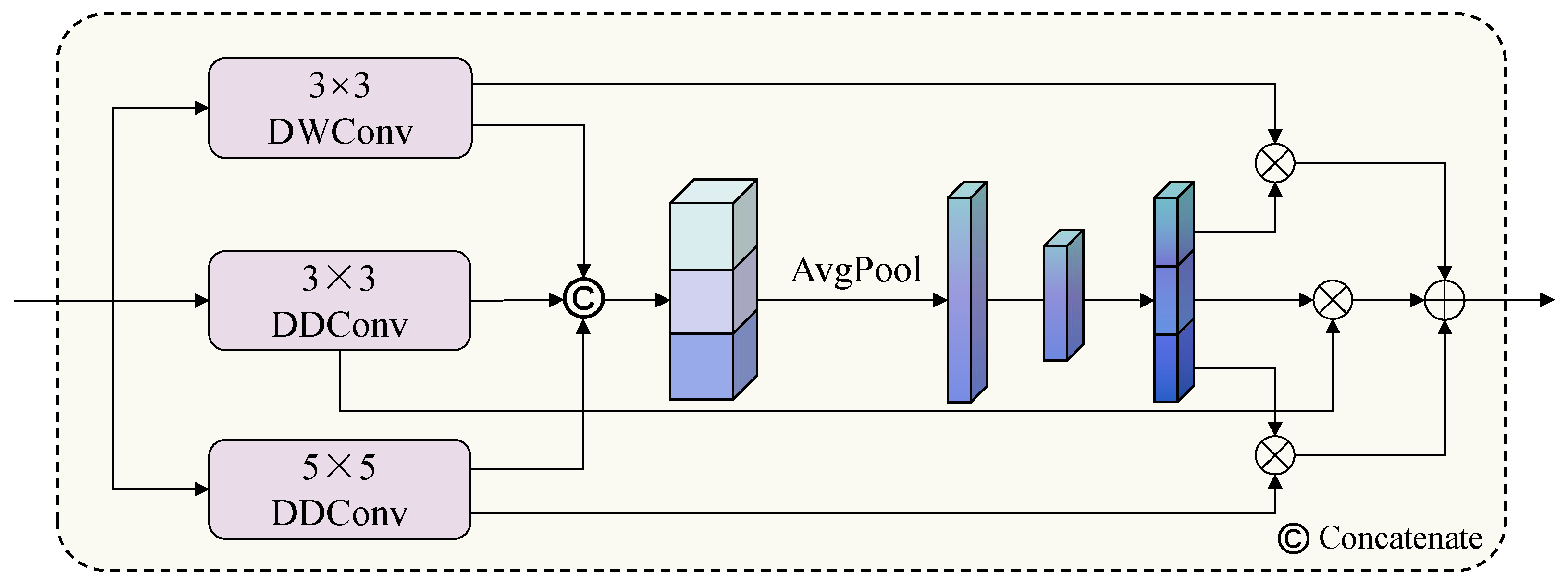
FusionSSM improves the SSM computation process by incorporating the innovative Multi-Scale Feature Fusion Module (MSFM) after the state transition equation, which facilitates the flow of spatial context information and alleviates the limitations imposed by causal relationships.

3.

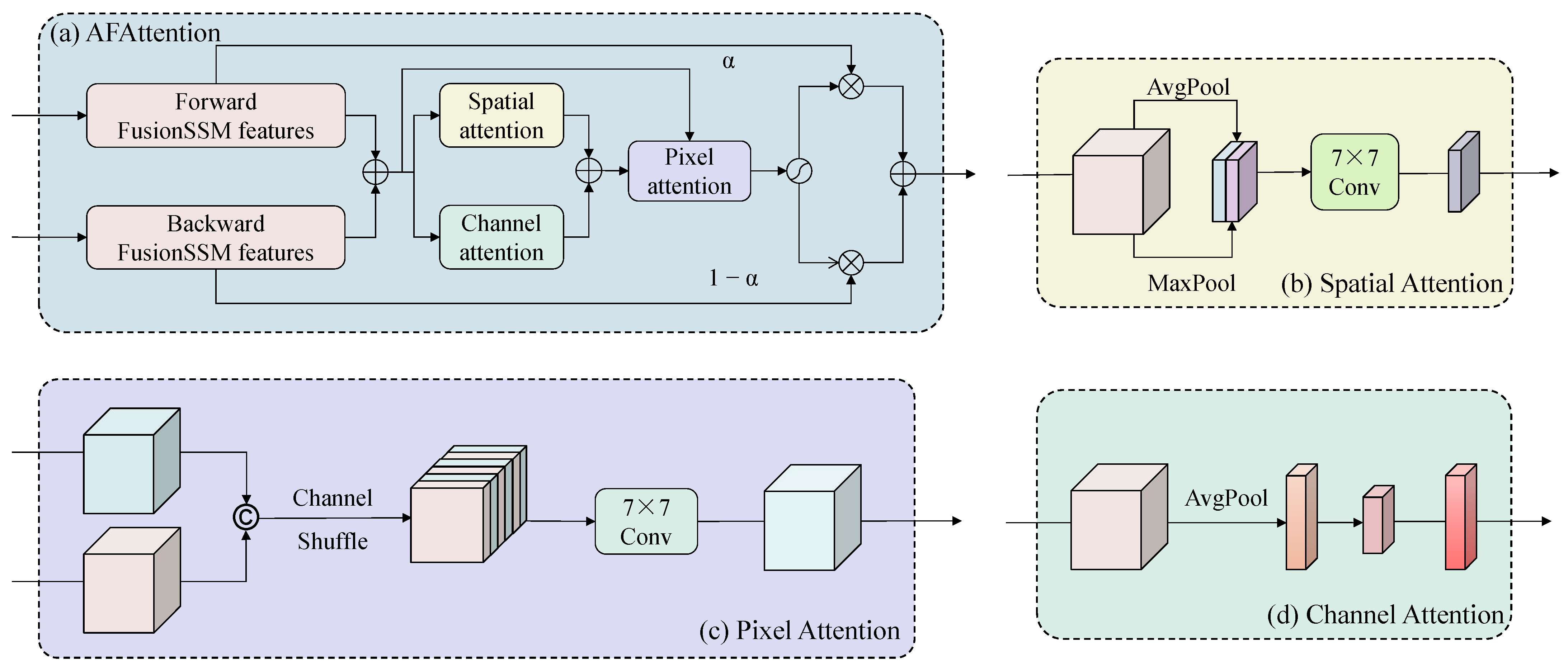
The Adaptive Fusion Attention Module (AFAttention) is proposed to interact and fuse multi-source spatial–spectral features, allowing the model to autonomously focus on key feature regions.

2. Methods

2.1. Overview

In order to achieve collaborative deep mining of spectral features in HSI, this study develops the end-to-end framework HyperSMamba, as illustrated in Figure 1.

We first apply principal component analysis (PCA) [40] to obtain a reduced representation $I\in {\mathbb{R}}^{H\times W\times C}$, where H, W, and C represent the height, width, and the number of retained principal components. Then, we adopt the Follow Patch method proposed by Yang et al. [41] to divide the reduced HSI into localized 3D patches $X\in {\mathbb{R}}^{P\times P\times C}$, where P denotes the patch size. Unlike traditional padding-based or Vision Transformer (ViT)-style patches, this approach ensures that the target pixel is positioned as close to the center of the patch as possible, thus retaining more effective neighborhood information. To further exploit neighborhood dependencies, we apply horizontal forward and backward scanning to each patch, generating two directional sequences $x\left(t\right)\in {\mathbb{R}}^{P^2\times C}$.These sequences are then independently fed into the Multi-Scale Spatial Mamba (MS-Mamba) module for bidirectional spatial feature extraction. In MS-Mamba, the state variables computed from the state transition equations of the original SSM are reshaped into a visual format. The MSFM module is then employed to autonomously select meaningful neighboring state information to update each state variable, thereby enhancing spatial interaction. To further enhance feature fusion capability, we propose the AFAttention module, which integrates features extracted from forward and backward sequences. This module consists of spatial attention, channel attention, and pixel-wise attention mechanisms. We assign a unique importance weight to each pixel to refine forward and backward features, effectively reducing redundant information while preserving critical features unchanged. Finally, the improved features are supplied to the fully connected layer after being residually merged with the original and linearly modified features.

2.2. State-Space Models

The structured State-Space Sequence Model originates from the Kalman filter framework and excels at catching long-range relationships while demonstrating efficient parallel processing capabilities [42]. Through a learnable hidden state $h\left(t\right)\in {\mathbb{R}}^N$, the model converts a 1D input sequence $x\left(t\right)$ into an output sequence $y\left(t\right)\in {\mathbb{R}}^L$, where t indicates the time step, N and L denote the dimensions of the latent space and the sequence.

$$\tilde{h}\left(t\right)=Ah\left(t\right)+Bx\left(t\right),$$

(1)

$$y\left(t\right)=C\tilde{h}\left(t\right)+Dx\left(t\right).$$

(2)

The state transition equation describes the temporal dynamics of the hidden state, governed by its current value and the external input. Specifically, $A\in {\mathbb{R}}^{N\times N}$ is the state transition matrix, representing the transition relationship from the current state to the next state. $B\in {\mathbb{R}}^{N\times L}$ denotes the input projection matrix, capturing the influence of external inputs on the hidden state. $\tilde{h}\left(t\right)={\displaystyle \frac{dh\left(t\right)}{dt}}$ represents the time derivative of $h\left(t\right)$. The output equation generates $y\left(t\right)$ by projecting the updated hidden state into the output space via the observation matrix $C\in {\mathbb{R}}^{L\times N}$, while D acts as a residual connection, often omitted in practical implementations.

To adapt this continuous system for discrete sequence data, the Zero-Order Hold (ZOH) rule is applied to discretize the continuous parameters. The ZOH rule approximates inputs as constant within each sampling interval, ensuring consistency between the continuous model and its discrete-time implementation.

$$\overline{A}=exp(\Delta A),$$

(3)

$$\overline{B}={(\Delta A)}^{-1}\left(exp(\Delta A)-I\right)·\Delta B.$$

(4)

Specifically, a time scaling parameter $\Delta \in {\mathbb{R}}^L$ is introduced. Here, $exp(·)$ denotes the matrix exponential function, which propagates the system dynamics over a time interval $\Delta$, and I represents the identity matrix. The matrices $\overline{A}\in {\mathbb{R}}^{N\times N}$ and $\overline{B}\in {\mathbb{R}}^{N\times L}$ are the discretized forms of A and B. After discretization, the state-space model equations are shown below:

$$h\left(t\right)=\overline{A}h(t-1)+\overline{B}x\left(t\right),$$

(5)

$$y\left(t\right)=Ch\left(t\right)+Dx\left(t\right).$$

(6)

However, Gu et al. [43] pointed out that the matrices A, B, and C in traditional state-space models typically remain fixed throughout the entire sequence, thereby exhibiting Linear Time Invariance (LTI). This property limits the model’s expressiveness when dealing with complex, dynamically changing sequence patterns. To overcome this limitation, Mamba introduces a selective scanning mechanism, allowing parameters to change with input, improving the model’s capacity in dynamic contexts. Additionally, Mamba adopts a hardware-efficient parallel implementation to resolve the inference latency bottlenecks observed in S4, marking a notable advancement in the evolution of state-space models.

2.3. Multi-Scale Spatial Mamba

Since the state transition equation of Mamba is influenced solely by the past and current input states within the sequence, the model is unable to leverage information from unscanned data. This limitation restricts its receptive field and impairs its ability to capture global contextual information, potentially leading to incomplete or biased feature representations.

To establish spatial dependencies with unscanned adjacent features, we introduce Multi-Scale Spatial Mamba (MS-Mamba). In this module, FusionSSM incorporates the Multi-Scale State Fusion Module (MSFM) into the original Mamba structure. It performs self-learning weighting of adjacent state variables to aggregate information from neighboring states, thereby enhancing the representation of spatial relational features.

As depicted in Figure 1, each sequence is processed through a 1D convolutional (1D-CNN) layer and SiLU activation function. Subsequently, the FusionSSM module captures long-range dependencies while simultaneously incorporating latent local spatial information. The overall process of FusionSSM can be described by three equations: the state transition equation, the MSFM, and the observation equation.

$$h\left(t\right)=\overline{A}h(t-1)+\overline{B}x\left(t\right),$$

(7)

$$h^{\prime }\left(t\right)=MSFM\left(h\left(t\right)\right),$$

(8)

$$y\left(t\right)=C{h}^{\prime }\left(t\right)+Dx\left(t\right).$$

(9)

Specifically, the current state $h\left(t\right)$ is first computed using the state transition equation of the original SSM and then reshaped into a visualizable format. To enable each state to perceive its neighboring states, we employ the MSFM module to perform Multi-Scale State Fusion on the processed state variables. This procedure integrates local dependency information into the new state $h^{\prime }\left(t\right)$, resulting in a more contextually informed representation. Then, the new state variables $h^{\prime }\left(t\right)$ are reverted to the original format and fed to the observation equation to compute the final result. Finally, the resulting output from the observation equation is multiplied by a Gaussian decay mask to optimize the feature distribution, yielding the forward features $X_{\mathrm{for}}\in {\mathbb{R}}^{P\times P\times C}$ and backward features $X_{\mathrm{back}}\in {\mathbb{R}}^{P\times P\times C}$.

2.4. Multi-Scale State Fusion Module

Hyperspectral images present local spatial heterogeneity, meaning that the same land cover class may exhibit different spectral responses at different spatial locations. Traditional CNNs, owing to the restricted local receptive field, often struggle to fully extract effective features [44]. Moreover, convolutional features extracted at different scales possess varying degrees of importance, and simple fusion strategies fail to fully exploit their complementary characteristics. Therefore, it is essential to design a model that can effectively extract spatial features at multiple scales and adaptively fuse them based on their contextual relevance.

We introduce the Multi-Scale State Fusion Module (MSFM), designed to dynamically select spatial features at various scales through multi-scale convolutions, as shown in Figure 2.

The MSFM module adopts a parallel three-branch convolution architecture. For input $X_{in}$, the first branch uses standard depthwise convolution (DWConv) to capture fine-grained local features. The second and third branches utilize depthwise dilated convolutions (DDConv) with different kernel sizes to approximate the receptive field of large kernel convolutions, identifying regions with similar local features but more distant distributions. Then, a richer feature representation $X_{\mathrm{concat}}$ is created by concatenating the outputs of three branches along the channel dimension.

$$X_{\mathrm{concat}}=Concat({DWConv}_{3\times 3}\left(X_{\mathrm{in}}\right),{DDConv}_{5\times 5}\left(X_{\mathrm{in}}\right),{DDConv}_{7\times 7}\left(X_{\mathrm{in}}\right)).$$

(10)

Here, ${DDConv}_{k\times k}(·)$ and ${DWConv}_{k\times k}(·)$ denote dilated depthwise convolution and standard depthwise convolution using a $k\times k$ convolutional kernel. The operator $Concat(·)$ performs channel-wise concatenation.

Next, we use the average pooling layer and two convolutional layers to calculate the attention weights of the feature map, guiding the model to learn the interactions between channels at different scales during the fusion process. Finally, these attention weights are applied to the convolutional inputs of the corresponding scales to achieve weighting of the important channels and help the model automatically focus on more representative features.

$$[W_1;W_2;W_3]={Conv}_{1\times 1}\left({Conv}_{1\times 1}\left(AvgPool\left(X_{\mathrm{concat}}\right)\right)\right),$$

(11)

$$h^{\prime }\left(t\right)=W_1·{DWConv}_{3\times 3}\left(X_{\mathrm{in}}\right)+W_2·{DDConv}_{3\times 3}\left(X_{\mathrm{in}}\right)+W_3·{DDConv}_{5\times 5}\left(X_{\mathrm{in}}\right).$$

(12)

Here, $AvgPool(·)$ represents the average pooling, ${Conv}_{1\times 1}(·)$ is a point-wise convolutional layer used for channel compression and attention extraction. $[W_1;W_2;W_3]$ represents the learned attention weights corresponding to three convolutional branches. The final output $h^{\prime }\left(t\right)$ is the weighted sum of the three convolutional paths.

2.5. Adaptive Fusion Attention Module

To more effectively integrate key information from the forward and backward features while suppressing redundant and noisy components, we designed the Adaptive Fusion Attention Module (AFAttention), as illustrated in Figure 3. The module dynamically evaluates the relative importance of forward and backward features, achieving intelligent control of the bidirectional feature flow. AFAttention is composed of spatial attention, channel attention, and pixel attention.

We perform element-wise addition of the forward features $X_{\mathrm{for}}\in {\mathbb{R}}^{P\times P\times C}$ and backward features $X_{\mathrm{back}}\in {\mathbb{R}}^{P\times P\times C}$ to obtain $X_{\mathrm{sum}}\in {\mathbb{R}}^{P\times P\times C}$. Subsequently, $X_{\mathrm{sum}}$ is fed into the spatial attention and channel attention, which generate spatial attention weights $W_{\mathrm{s}}\in {\mathbb{R}}^{P\times P\times 1}$ and channel attention weights $W_{\mathrm{c}}\in {\mathbb{R}}^{1\times 1\times C}$, respectively.

The spatial attention (Figure 3b) applies max pooling and average pooling along the channel dimension. These pooled features are concatenated and processed by a $7\times 7$ convolutional layer, capturing important features from local regions and enhancing the model’s spatial discriminative ability.

The channel attention (Figure 3d) compresses spatial dimensions using global average pooling and generates channel weights through a series of nonlinear transformations. This mechanism helps enhance the critical spectral band information in hyperspectral data while suppressing redundant channels. Subsequently, $W_{\mathrm{s}}$ and $W_{\mathrm{c}}$ are fused together through simple addition to generate the spatial–spectral importance matrix $W_{\mathrm{sc}}\in {\mathbb{R}}^{P\times P\times C}$.

$$W_s={Conv}_{7\times 7}\left(\left[AvgPool\left(X_{\mathrm{sum}}\right);MaxPool\left(X_{\mathrm{sum}}\right)\right]\right),$$

(13)

$$W_c=W_1\left(W_0(AvgPool\left(X_{\mathrm{sum}}\right))\right),$$

(14)

$$W_{sc}=W_s+W_c.$$

(15)

Here, ${Conv}_{7\times 7}$ represents a convolution operation with a $7\times 7$ kernel, and MaxPool refers to channel-wise max pooling. $W_0\in {\mathbb{R}}^{C\times C/r}$, $W_1\in {\mathbb{R}}^{C/r\times C}$ are nonlinear transformation coefficients.

Finally, we use pixel attention (Figure 3c) to obtain the final pixel attention matrix W and apply $X_{\mathrm{s}\mathrm{u}\mathrm{m}}$ as guidance to adaptively adjust each channel of $W_{\mathrm{s}\mathrm{c}}$. Specifically, each channel of $W_{\mathrm{s}\mathrm{c}}$ and $X_{\mathrm{s}\mathrm{u}\mathrm{m}}$ is rearranged in an alternating manner through Channel Shuffle [45] and fused using a $7\times 7$ group convolution that allows for full interaction of information from different sources. Then, the attention weights are normalized using the sigmoid activation to obtain the final weights W.

$$W=\sigma \left({GConv}_{7\times 7}(CS\left([X_{\mathrm{sum}},W_{\mathrm{sc}}]\right))\right).$$

(16)

where ${GConv}_{7\times 7}(·)$ denotes a grouped convolution operation with a $7\times 7$ kernel. $CS(·)$ is a channel rearrangement operation. $\sigma (·)$ represents the sigmoid activation function.

Due to the different importance of forward and backward features, they are separately element-wise multiplied with the pixel attention matrix W and then combined using the weighted average method with the self-learned parameter $\alpha$.

$$y_{\mathrm{output}}=\alpha ·(X_{\mathrm{for}}\odot W)+(1-\alpha )·(X_{\mathrm{back}}\odot W)$$

(17)

where ⊙ denotes element-wise dot multiplication, $y_{\mathrm{output}}$ is the final result of the model.

3. Results

3.1. Datasets Description

To systematically evaluate the model, we conduct comprehensive evaluations on three commonly used HSI datasets. The sample distribution is detailed in

Table 1. Description of land cover types and number of train–test samples in the Indian Pines dataset.

Class ID	Category	Training	Testing	Total
1	Alfalfa	15	31	46
2	Corn-notill	40	1388	1428
3	Corn-mintill	40	790	830
4	Corn	40	197	237
5	Grass-pasture	40	443	483
6	Grass-trees	40	690	730
7	Grass-pasture-mowed	15	13	28
8	Hay-windrowed	40	438	478
9	Oats	15	5	20
10	Soybeans-notill	40	932	972
11	Soybean-mintill	40	2415	2455
12	Soybean-clean	40	553	593
13	Wheat	40	165	205
14	Woods	40	1225	1265
15	Build-grass-trees-drivers	40	346	386
16	Stones-steel-towers	40	53	93
	Total	565	9684	10,249

,

Table 2. Description of land cover types and number of train–test samples in the Pavia University dataset.

Class ID	Category	Training	Testing	Total
1	Asphalt	30	6601	6631
2	Meadows	30	18,619	18,649
3	Gravel	30	2069	2099
4	Trees	30	3034	3064
5	Metal Sheets	30	1315	1345
6	Bare-soil	30	4999	5029
7	Bitumen	30	1300	1300
8	Bricks	30	3652	3682
9	Shadows	30	917	947
	Total	270	42,506	42,776

and

Table 3. Description of land cover types and number of train–test samples in the Salinas dataset.

Class ID	Category	Training	Testing	Total
1	Brocoli_green_weeds_1	30	1979	2009
2	Brocoli_green_weeds_2	30	3696	3726
3	Fallow	30	1946	1976
4	Fallow_rough_plow	30	1364	1394
5	Fallow_smooth	30	2648	2678
6	Stubble	30	3929	3959
7	Celery	30	3549	3579
8	Grapes_untrained	30	11,241	11,271
9	Soil_vinyard_develop	30	6173	6203
10	SCorn_senesced_green_weeds	30	3248	3278
11	Lettuce_romaine_4wk	30	1038	1068
12	Lettuce_romaine_5wk	30	1897	1927
13	Lettuce_romaine_6wk	30	886	916
14	Lettuce_romaine_7wk	30	1040	1070
15	Vinyard_untrained	30	7238	7268
16	Vinyard_vertical_trellis	30	1777	1807
	Total	480	53,649	54,129

.

1.

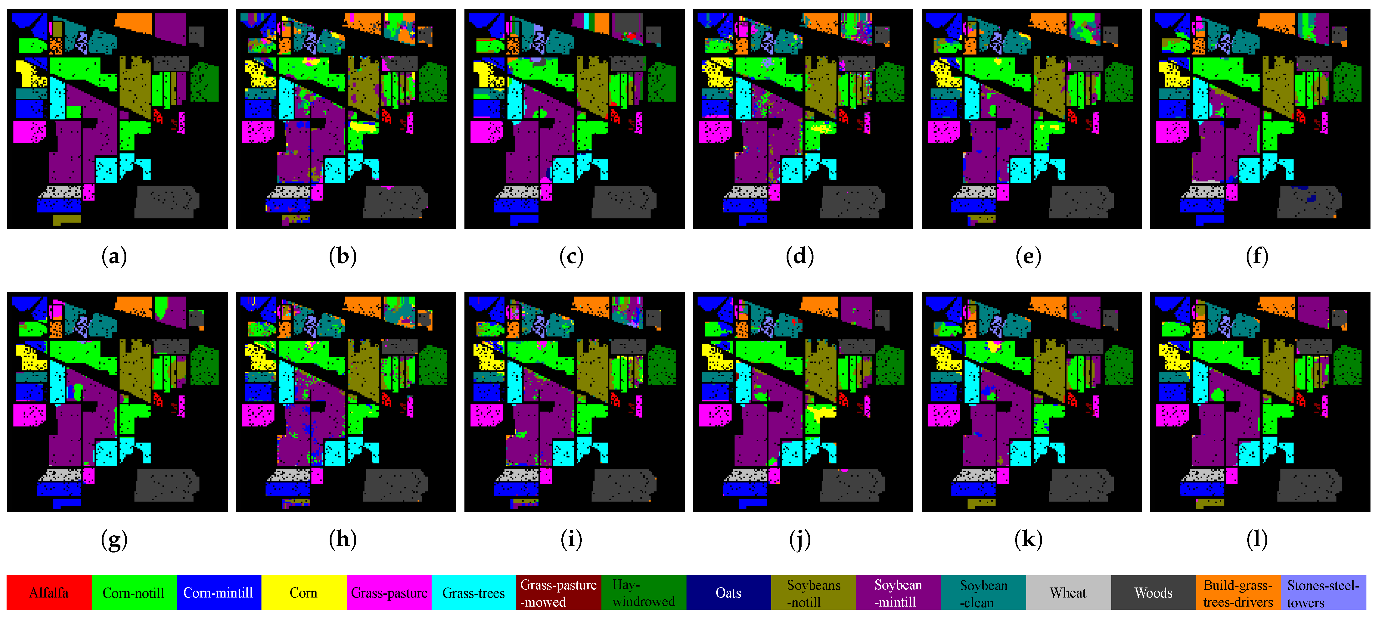
Indian Pines (IP): The IP dataset was collected from the agricultural region of Indiana, USA, and contains $145\times 145$ pixels. 200 valid bands were retained, covering wavelengths from 400 nm to 2500 nm. The dataset covers 16 different land cover types.

2.

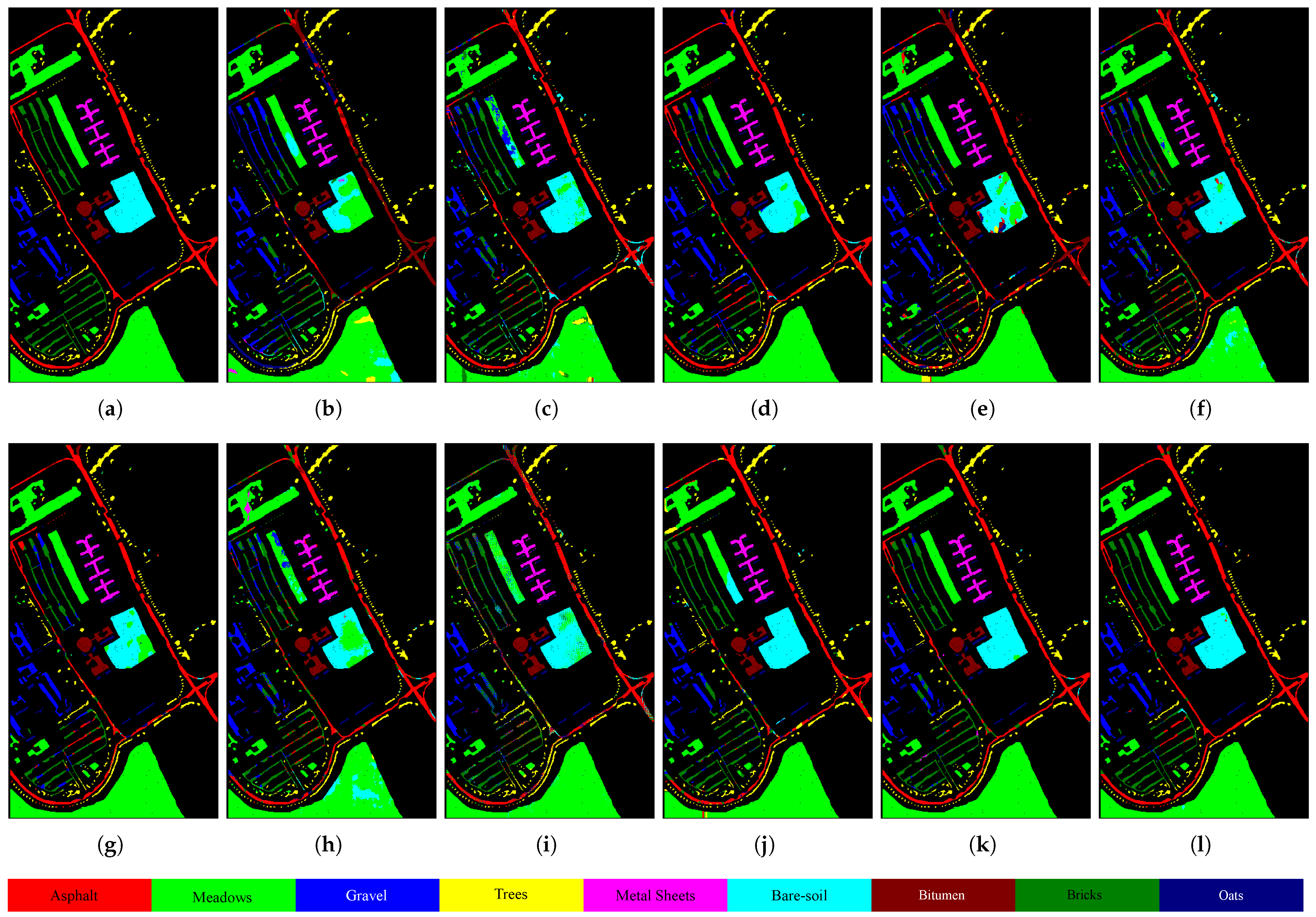
Pavia University (UP): The UP dataset was collected from the University of Pavia, Italy. It consists of $610\times 340$ pixels and a total of 103 spectral bands. The dataset covers nine different land cover types.

3.

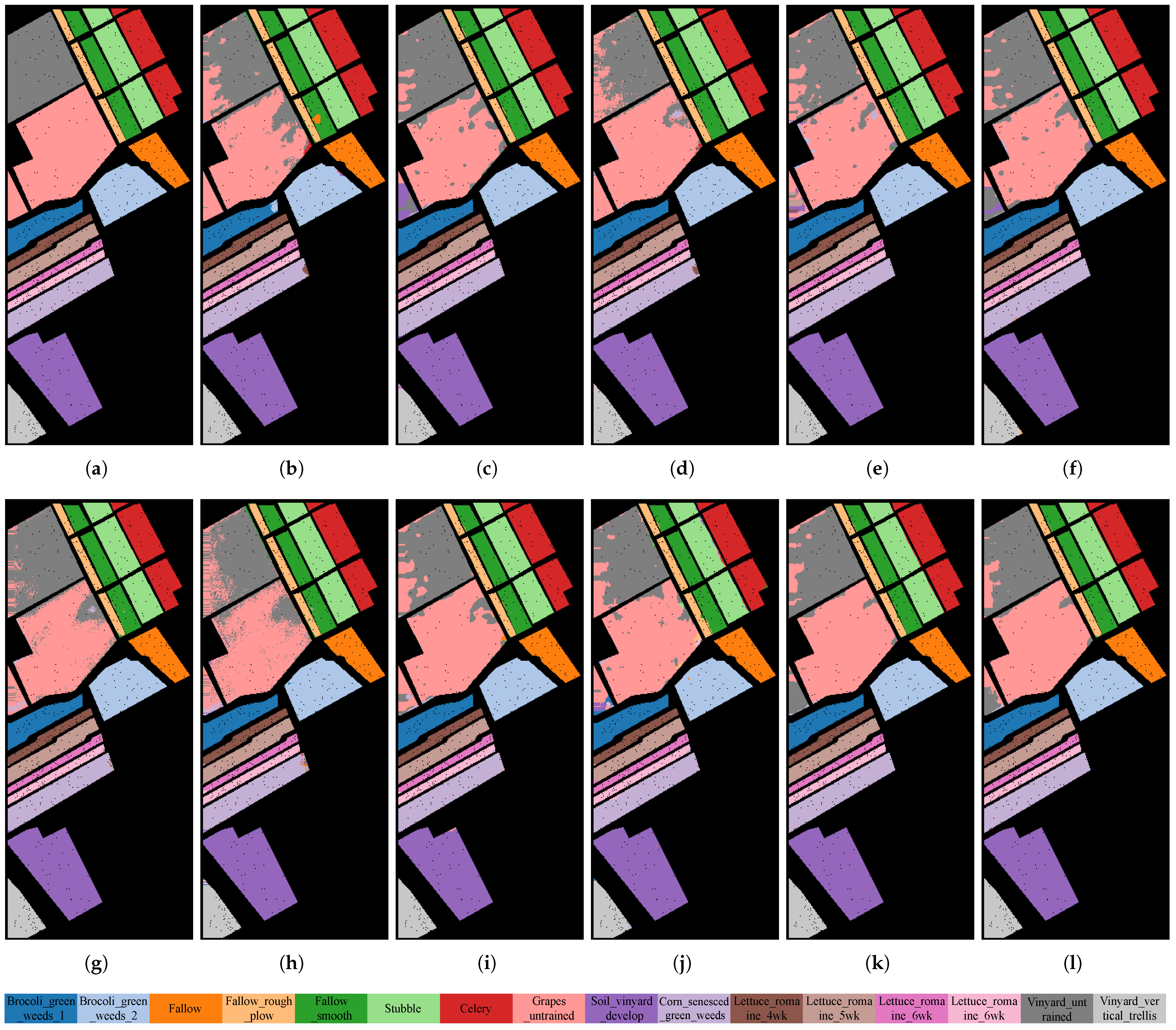
Salinas (SA): This dataset was collected from the Salinas region of California, USA. The HSI size is $512\times 217$ pixels, covering 16 land cover types. After preprocessing, 204 valid bands were retained.

3.2. Experimental Setup

1.

Implementation Details: All models are implemented using PyTorch 2.5 and trained on an NVIDIA Tesla T4 GPU (16 GB VRAM). The batch size for all models is set to 128, and the number of epochs is set to 400. We use the cross-entropy loss function to update parameters. The AdamW optimizer is used with an initial learning rate of $5\times {10}^{-4}$. In the proposed HyperSMamba model, all feature dimensions are normalized to 50. The initial patch sizes are set to $9\times 9$ for the Indian Pines (IP) dataset and $11\times 11$ for both the Pavia University (UP) and Salinas (SA) datasets. To ensure reproducibility of the results, the random seed was fixed, and each experiment was repeated 10 times.

2.

Evaluation Metrics: We adopt three standard evaluation metrics, including average accuracy (AA), overall accuracy (OA), and Kappa coefficient $\left(\kappa \right)$.

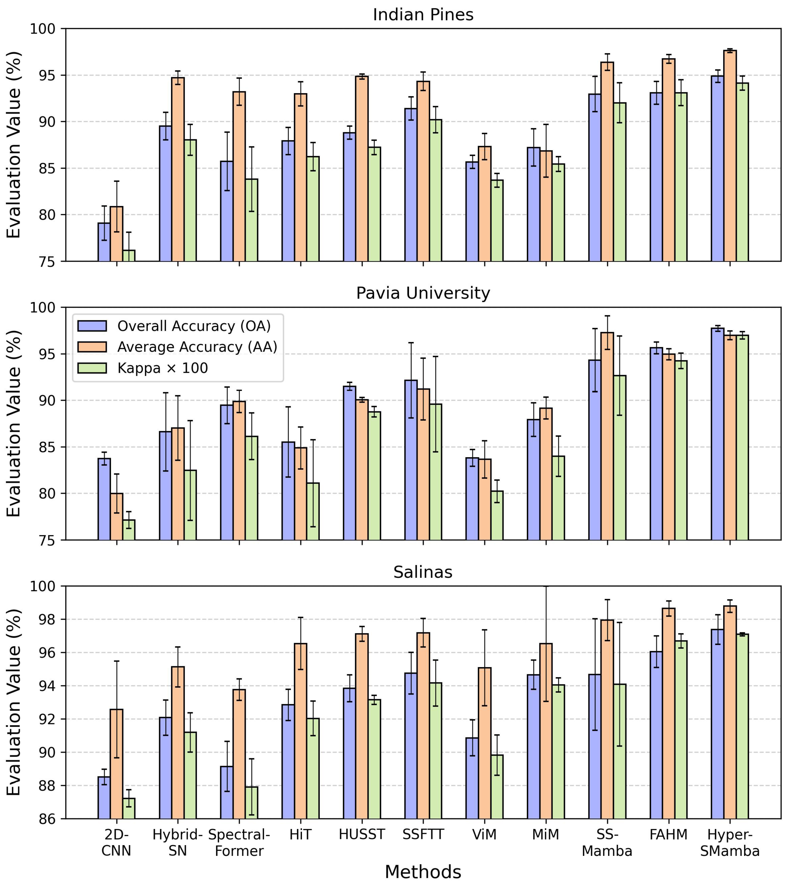
3.3. Comparative Experimentation

3.3.1. Contrast Experiment Results

In order to evaluate the effectiveness of the proposed method, we conducted a comparative analysis against a series of baselines. These models include 2D-CNN [46], HybridSN [17], SpectralFormer [19], HiT [24], HUSST [25], SSFTT [23], and SSM-based ViM [28], MiM [36], SSMamba [37], and FAHM [35]. All models were tested under the optimal experimental conditions. Details can be found in the original paper.

Table 4. Quantitative performance of different classification methods in terms of OA (%), AA (%), scaled $\kappa$ ($\times 100$), and per-class accuracy (%) on the Indian Pines dataset. The best results are highlighted in bold.

Class No.	2D CNN	Hybrid SN	Spectral Former	HiT	HUSST	SSFTT	ViM	MiM	SS- Mamba	FAHM	Hyper- SMamba
1	86.21 ± 3.34	92.83 ± 6.30	97.29 ± 3.27	85.05 ± 2.35	80.88 ± 1.87	89.13 ± 9.82	89.79 ± 5.05	95.65 ± 7.49	99.38 ± 1.88	95.90 ± 4.08	99.10 ± 1.24
2	71.86 ± 2.13	86.76 ± 1.88	79.15 ± 2.74	81.89 ± 1.42	82.16 ± 0.94	88.94 ± 2.17	77.44 ± 1.30	83.40 ± 8.83	83.65 ± 5.73	88.78 ± 2.00	89.99 ± 2.04
3	69.52 ± 2.53	90.27 ± 2.93	85.73 ± 4.01	85.59 ± 0.92	87.55 ± 1.65	88.36 ± 2.92	82.19 ± 2.49	78.80 ± 6.94	92.10 ± 3.60	95.49 ± 1.22	92.88 ± 1.31
4	64.92 ± 6.21	88.17 ± 5.16	80.41 ± 4.94	86.42 ± 1.73	92.52 ± 0.92	92.72 ± 5.44	84.04 ± 2.99	77.64 ± 10.26	99.23 ± 2.16	93.10 ± 4.16	94.54 ± 2.29
5	80.43 ± 3.75	91.10 ± 2.52	93.02 ± 3.38	89.74 ± 1.12	95.37 ± 0.97	92.28 ± 1.93	88.53 ± 3.62	86.13 ± 3.26	94.06 ± 1.91	97.00 ± 1.89	97.81 ± 1.12
6	93.23 ± 0.98	95.20 ± 3.67	98.63 ± 0.62	95.02 ± 0.73	97.75 ± 0.36	95.30 ± 3.03	95.54 ± 1.05	96.30 ± 0.78	98.89 ± 0.49	98.88 ± 0.71	99.42 ± 0.26
7	81.67 ± 5.77	90.80 ± 9.63	88.22 ± 9.25	89.12 ± 5.10	95.44 ± 4.27	75.86 ± 2.64	93.43 ± 4.63	82.14 ± 7.14	100.00 ± 0.00	91.48 ± 8.36	95.32 ± 2.68
8	95.63 ± 0.38	99.24 ± 0.86	99.31 ± 0.77	96.87 ± 0.49	99.39 ± 0.59	98.45 ± 1.14	96.59 ± 0.61	98.95 ± 0.63	100.00 ± 0.00	99.75 ± 0.34	100.00 ± 0.00
9	70.18 ± 12.24	72.90 ± 19.62	73.92 ± 14.07	60.29 ± 9.04	77.14 ± 8.11	51.29 ± 32.91	74.60 ± 14.11	70.00 ± 0.15	100.00 ± 0.00	93.22 ± 1.99	94.87 ± 4.74
10	66.41 ± 3.17	80.88 ± 4.28	78.85 ± 6.70	78.00 ± 1.01	79.93 ± 1.37	83.51 ± 1.40	74.11 ± 2.07	82.10 ± 5.25	91.15 ± 4.76	94.03 ± 3.08	90.58 ± 0.78
11	76.38 ± 2.08	86.49 ± 2.44	80.25 ± 5.62	88.99 ± 1.21	84.74 ± 1.35	91.68 ± 1.76	86.07 ± 1.06	84.93 ± 5.37	89.81 ± 5.09	91.33 ± 2.45	91.72 ± 2.83
12	68.28 ± 5.07	87.42 ± 3.37	72.95 ± 4.46	79.06 ± 2.24	83.53 ± 2.34	91.24 ± 4.21	79.84 ± 1.96	84.49 ± 4.89	94.07 ± 4.20	93.92 ± 4.26	94.34 ± 0.99
13	95.03 ± 1.95	97.08 ± 2.35	98.40 ± 2.23	96.70 ± 0.80	98.80 ± 0.58	96.40 ± 2.58	94.81 ± 1.30	95.61 ± 3.16	100.00 ± 0.00	99.64 ± 0.55	97.71 ± 1.58
14	96.14 ± 1.05	97.37 ± 1.03	97.81 ± 0.64	97.22 ± 0.35	98.82 ± 0.28	97.30 ± 0.94	96.40 ± 0.54	96.60 ± 1.42	98.86 ± 0.64	98.74 ± 0.97	99.35 ± 0.35
15	85.14 ± 7.14	89.30 ± 2.70	88.70 ± 4.10	90.77 ± 1.77	95.60 ± 1.19	92.26 ± 4.80	86.84 ± 3.17	91.71 ± 2.60	97.33 ± 2.46	98.13 ± 1.45	97.82 ± 1.57
16	80.49 ± 3.13	88.42 ± 10.33	86.80 ± 8.83	63.85 ± 2.60	89.34 ± 2.11	81.54 ± 4.58	70.19 ± 5.66	84.95 ± 7.98	99.05 ± 1.05	90.92 ± 2.36	95.75 ± 3.68
OA (%)	79.06 ± 1.84	89.50 ± 1.48	85.69 ± 3.14	87.89 ± 1.47	88.79 ± 0.69	91.38 ± 1.25	85.64 ± 0.71	87.20 ± 1.99	92.94 ± 1.91	93.06 ± 1.23	94.86 ± 0.67
AA (%)	80.84 ± 2.73	94.70 ± 0.72	93.18 ± 1.46	92.96 ± 1.30	94.83 ± 0.27	94.31 ± 1.00	87.30 ± 1.41	86.83 ± 2.84	96.37 ± 0.88	96.71 ± 0.46	97.60 ± 0.20
$\kappa \times 100$	76.13 ± 1.96	88.02 ± 1.67	83.79 ± 3.45	86.21 ± 1.52	87.21 ± 0.77	90.17 ± 1.41	83.67 ± 0.74	85.41 ± 0.79	92.00 ± 2.16	93.07 ± 1.39	94.13 ± 0.76

,

Table 5. Quantitative performance of different classification methods in terms of OA (%), AA (%), scaled $\kappa$ ($\times 100$), and per-class accuracy (%) on the Pavia University dataset. The best results are highlighted in bold.

Class No.	2D CNN	Hybrid SN	Spectral Former	HiT	HUSST	SSFTT	ViM	MiM	SS- Mamba	FAHM	Hyper- SMamba
1	77.86 ± 1.48	75.40 ± 6.38	88.55 ± 2.57	78.53 ± 5.71	84.75 ± 1.51	89.42 ± 7.15	75.39 ± 2.31	85.99 ± 2.04	94.14 ± 3.47	95.64 ± 1.36	96.77 ± 0.58
2	88.67 ± 0.89	94.62 ± 3.70	94.80 ± 1.55	94.07 ± 2.78	97.64 ± 0.36	96.95 ± 2.16	94.78 ± 0.64	87.17 ± 1.59	90.31 ± 7.34	98.95 ± 0.39	99.66 ± 0.10
3	80.59 ± 6.18	76.78 ± 6.06	72.20 ± 4.50	75.63 ± 7.43	87.60 ± 1.12	85.69 ± 6.35	73.61 ± 2.73	83.46 ± 7.35	93.67 ± 11.98	95.44 ± 2.01	93.09 ± 1.67
4	79.70 ± 1.33	83.52 ± 4.80	93.69 ± 1.80	78.94 ± 5.04	77.36 ± 0.69	89.45 ± 2.11	81.08 ± 1.32	85.67 ± 5.55	99.09 ± 0.38	95.19 ± 1.08	95.15 ± 0.67
5	88.97 ± 1.89	99.33 ± 0.68	99.85 ± 0.06	97.88 ± 0.45	96.12 ± 0.32	98.59 ± 1.34	98.57 ± 0.22	99.33 ± 0.64	100.00 ± 0.00	98.16 ± 1.05	99.34 ± 0.10
6	85.29 ± 1.57	91.26 ± 5.46	84.87 ± 4.46	84.28 ± 5.93	95.28 ± 1.17	90.60 ± 6.17	84.87 ± 1.71	93.96 ± 4.37	99.43 ± 0.23	98.28 ± 1.32	99.58 ± 0.16
7	83.54 ± 1.82	87.51 ± 9.62	89.94 ± 2.71	93.23 ± 3.91	98.35 ± 0.46	94.84 ± 3.61	90.32 ± 3.51	95.64 ± 3.44	99.96 ± 0.12	98.40 ± 0.82	99.02 ± 0.78
8	61.33 ± 4.12	68.54 ± 7.09	73.30 ± 3.84	86.90 ± 4.35	79.49 ± 1.04	79.40 ± 7.27	66.93 ± 2.51	84.68 ± 2.47	98.15 ± 3.09	95.64 ± 2.24	92.23 ± 1.42
9	73.72 ± 1.90	68.72 ± 12.10	93.76 ± 2.93	65.30 ± 12.55	80.47 ± 1.81	85.17 ± 9.71	70.72 ± 3.79	86.38 ± 9.76	99.99 ± 0.03	94.24 ± 1.78	96.20 ± 1.06
OA (%)	83.72 ± 0.69	86.59 ± 4.20	89.45 ± 1.96	85.50 ± 3.77	91.49 ± 0.43	92.12 ± 4.04	83.80 ± 0.91	87.91 ± 1.81	94.30 ± 3.39	95.63 ± 0.63	97.72 ± 0.31
AA (%)	79.96 ± 2.09	87.01 ± 3.47	89.87 ± 1.19	84.86 ± 2.27	90.04 ± 0.26	91.18 ± 3.32	83.63 ± 2.01	89.15 ± 1.16	97.25 ± 1.80	94.94 ± 0.59	96.98 ± 0.47
$\kappa \times 100$	77.11 ± 0.91	82.44 ± 5.37	86.11 ± 2.51	81.07 ± 4.67	88.75 ± 0.55	89.56 ± 5.13	80.20 ± 1.20	83.98 ± 2.16	92.62 ± 4.26	94.21 ± 0.83	96.97 ± 0.41

and

Table 6. Quantitative performance of different classification methods in terms of OA (%), AA (%), scaled $\kappa$ ($\times 100$), and per-class accuracy (%) on the Salinas dataset. The best results are highlighted in bold.

Class No.	2D CNN	Hybrid SN	Spectral Former	HiT	HUSST	SSFTT	ViM	MiM	SS- Mamba	FAHM	Hyper- SMamba
1	99.51 ± 0.87	99.98 ± 0.02	94.19 ± 1.78	100.00 ± 0.00	100.00 ± 0.00	99.68 ± 0.56	96.84 ± 1.19	95.81 ± 0.12	100.00 ± 0.00	100.00 ± 0.00	99.99 ± 0.01
2	99.60 ± 0.53	99.93 ± 0.06	98.91 ± 0.08	99.34 ± 0.49	99.56 ± 0.26	99.65 ± 0.34	98.12 ± 1.01	99.95 ± 0.05	100.00 ± 0.00	99.97 ± 0.04	99.99 ± 0.01
3	98.59 ± 0.96	99.75 ± 0.24	92.02 ± 0.74	99.82 ± 0.16	99.99 ± 0.01	99.29 ± 1.17	99.22 ± 0.01	99.85 ± 0.02	99.86 ± 0.40	100.00 ± 0.00	100.00 ± 0.00
4	98.67 ± 0.33	98.61 ± 1.31	97.16 ± 1.25	97.49 ± 0.14	98.12 ± 0.42	95.79 ± 0.95	97.46 ± 0.65	96.48 ± 1.69	99.73 ± 0.31	98.92 ± 1.01	98.19 ± 0.89
5	97.37 ± 0.82	98.78 ± 0.81	89.23 ± 1.25	98.62 ± 0.22	98.48 ± 0.26	97.06 ± 2.16	97.97 ± 0.57	98.24 ± 1.01	97.87 ± 2.01	99.23 ± 0.33	99.42 ± 0.26
6	99.95 ± 0.05	99.68 ± 0.24	99.67 ± 0.55	99.43 ± 0.21	99.72 ± 0.13	98.13 ± 1.01	99.05 ± 0.30	98.38 ± 0.09	99.97 ± 0.03	99.52 ± 0.48	99.92 ± 0.06
7	99.59 ± 0.32	98.74 ± 0.71	97.80 ± 0.20	99.41 ± 0.23	99.47 ± 0.14	98.37 ± 1.04	98.98 ± 0.33	98.66 ± 0.07	99.83 ± 0.11	99.44 ± 0.52	99.93 ± 0.07
8	86.41 ± 1.54	90.29 ± 4.55	73.06 ± 2.47	83.58 ± 3.61	86.43 ± 1.50	89.16 ± 2.83	80.38 ± 4.70	88.66 ± 1.27	82.19 ± 17.65	93.37 ± 4.91	94.42 ± 2.14
9	99.84 ± 0.17	99.15 ± 0.60	98.76 ± 0.12	99.96 ± 0.02	99.97 ± 0.02	98.99 ± 1.11	97.96 ± 1.04	99.58 ± 0.06	99.99 ± 0.01	100.00 ± 0.00	99.83 ± 0.07
10	97.63 ± 1.06	96.27 ± 1.79	94.40 ± 1.65	99.49 ± 0.12	98.53 ± 0.64	96.44 ± 1.60	96.85 ± 1.44	97.53 ± 0.99	99.32 ± 0.64	99.73 ± 0.19	98.20 ± 1.09
11	98.65 ± 0.76	96.36 ± 1.51	98.73 ± 0.50	98.87 ± 0.02	98.72 ± 0.45	98.49 ± 1.76	98.70 ± 0.15	97.00 ± 1.71	99.74 ± 0.21	99.95 ± 0.05	98.60 ± 1.64
12	99.44 ± 0.50	98.67 ± 1.38	98.86 ± 0.48	98.46 ± 0.17	98.90 ± 0.35	97.37 ± 2.58	97.45 ± 0.25	97.09 ± 0.53	99.89 ± 0.33	99.94 ± 0.03	99.83 ± 0.15
13	98.81 ± 0.59	85.54 ± 5.56	97.86 ± 0.63	97.13 ± 0.54	98.39 ± 0.57	94.84 ± 3.31	96.10 ± 0.68	96.94 ± 1.02	99.86 ± 0.18	99.81 ± 0.13	99.47 ± 0.42
14	98.43 ± 0.56	97.40 ± 4.04	98.57 ± 0.87	97.76 ± 0.47	99.14 ± 0.16	93.05 ± 5.43	96.35 ± 0.62	96.54 ± 1.58	99.26 ± 0.95	99.31 ± 0.32	97.78 ± 1.74
15	79.16 ± 2.38	63.28 ± 3.25	78.46 ± 4.80	75.76 ± 4.13	78.58 ± 4.91	84.85 ± 2.48	72.26 ± 3.17	86.03 ± 1.93	89.56 ± 18.58	90.08 ± 5.41	91.49 ± 3.31
16	99.43 ± 0.15	99.49 ± 0.35	96.48 ± 0.34	99.11 ± 0.76	99.26 ± 0.34	98.82 ± 1.22	97.19 ± 1.01	97.34 ± 0.06	99.80 ± 0.28	99.87 ± 0.19	99.91 ± 0.16
OA (%)	88.50 ± 0.46	92.07 ± 1.06	89.13 ± 1.51	92.84 ± 0.94	93.84 ± 0.94	94.74 ± 1.25	90.85 ± 1.08	94.65 ± 0.88	94.66 ± 3.36	96.03 ± 0.95	97.38 ± 0.89
AA (%)	92.57 ± 2.91	95.12 ± 1.21	93.76 ± 0.65	96.53 ± 1.57	97.11 ± 0.45	97.18 ± 0.85	95.07 ± 2.29	96.52 ± 3.69	97.94 ± 1.24	98.64 ± 0.45	98.78 ± 0.37
$\kappa \times 100$	87.21 ± 0.52	91.18 ± 1.18	87.90 ± 1.69	92.02 ± 1.04	93.14 ± 0.27	94.15 ± 1.38	89.81 ± 1.21	94.04 ± 0.43	94.07 ± 3.72	96.69 ± 0.42	97.08 ± 0.10

show the average classification metrics and standard deviations of all comparison models after 10 experiments on three datasets. To further illustrate the comparative performance and stability of the proposed method, we include a detailed bar chart with error bars in Appendix A, Figure A1.

As a hybrid 2D–3D convolution-based method, HybridSN extracts joint local spectral–spatial features, thus outperforming certain Transformer-based methods. For example, on the IP and SA datasets, the classification accuracy of HybridSN is higher than SpectralFormer, which uses a Transformer only in the spectral dimension. SSFTT also utilizes 3D and 2D convolutions to extract information before the Transformer establishes long-range dependencies. This integrated spatial–spectral feature ensures that the Transformer receives inputs enriched with sufficient local semantic information. SSFTT achieves better performance than HiT, which embeds convolutions within the Transformer. The results illustrate that capturing local spatial features before establishing long-distance dependencies improves classification accuracy.

From the results, ViM does not perform well in hyperspectral image classification tasks. In contrast, MiM leverages the cross-sequence scanning mechanism to capture spatial information from four directions, leading to more focused and discriminative feature representations. Thus, MiM outperforms ViM in classification accuracy. SSMamba further extends the receptive field of spatial Mamba to large-scale $27\times 27$ token groups, while cross-band feature calibration is achieved through spectral Mamba, resulting in superior classification performance compared with MiM. In comparison, FAHM extracts both high-frequency and low-frequency features and improves the model’s capacity to capture contextual dependencies across spectral bands via bidirectional spectral analysis.

The proposed HyperSMamba model, built on ViM, does not enhance the ability to capture spatial neighborhood information by introducing cross-scanning sequences from additional directions. However, it still achieves excellent performance across all three datasets. Notably, on UP and SA datasets, the OA improves by 3.42% and 2.72%, compared with SSMamba, which confirms the proposed model’s superiority in HSIC tasks. Further analysis of the classification accuracy for each category reveals that HyperSMamba performs well on dominant categories and edge pixels. Although the classification accuracy for partly minor categories is sub-optimal, it remains stable and does not lead to serious misclassification due to data imbalance, and the overall performance is balanced. Additionally, as shown in Appendix A, Figure A1, the standard deviation of HyperSMamba’s classification metrics on all datasets is very small, which indicates that the algorithm’s classification performance is more balanced on all datasets, and it is able to maintain high robustness under different data distributions.

3.3.2. Visual Analysis of Classification Results

To facilitate an intuitive comparison of the performance across various classification methods, this study visualizes and analyzes the classification results. Figure 4, Figure 5 and Figure 6 show the classification visualization maps for the IP, UP, and SA datasets.

From the classification maps, it is evident that convolution-based models are significantly limited by local receptive fields, which hinders their ability to capture global spatial context. This limitation results in reduced classification accuracy at category boundaries and disrupts spatial consistency. The Transformer-based models possess global modeling capabilities, which make the category edge transition smoother and provide a clearer distinction between flat land cover areas and boundaries. However, the under-utilization of spatial information in small-scale areas leads to misclassification of fine-grained categories and loss of texture information, which affects overall classification performance.

Compared with other methods, HyperSMamba effectively extracts both local and global spatial features. Across multiple datasets, it demonstrates superior texture discrimination and boundary recognition ability. The classification maps produced by HyperSMamba exhibit smoother visual transitions, sharper inter-class boundaries, and significantly reduced misclassification errors.

3.4. Ablation Study

3.4.1. Ablation for the HyperSMamba Architecture

To assess the contribution of the MSFM and AFAttention modules to the performance of the proposed HyperSMamba model, we conducted ablation experiments. The results are summarized in

Table 7. Ablation study on the impact of different modules in HyperSMamba on OA (%), AA (%), and scaled $\kappa$ ($\times 100$) across three datasets. The best results are highlighted in bold.

MSFM	AFAttention	Indian Pines			Pavia University			Salinas
		OA (%)	AA (%)	$\mathit{\kappa }\times \mathbf{100}$	OA (%)	AA (%)	$\mathit{\kappa }\times \mathbf{100}$	OA (%)	AA (%)	$\mathit{\kappa }\times \mathbf{100}$
×	×	86.49	88.49	85.21	85.97	86.13	82.68	94.02	97.40	94.08
×	✔	90.64	94.23	89.58	93.92	92.94	92.91	96.44	98.54	96.04
✔	×	92.86	96.61	91.62	96.67	95.67	95.59	96.82	98.68	96.46
✔	✔	94.86	97.60	94.13	97.72	96.98	96.97	97.38	98.78	97.08

.

The inclusion of MSFM significantly improves the evaluation metrics across all three datasets. This finding indicates that this component can partially compensate for the loss of spatial structural information caused by flattening the input into 1D sequences. By integrating local spatial context into the latent state representation, MSFM improves spatial feature representation.

The AFAttention module adaptively adjusts the importance of spatial and channel features, optimizing the complementary relationship between bidirectional states and enhancing both feature fusion quality and classification accuracy. The accuracy of all datasets improved after adding the attention fusion module, further confirming the effectiveness of the AFAttention module.

When both MSFM and AFAttention are incorporated, the model benefits from enhanced global context modeling, as well as multi-scale spatial feature extraction. The ablation results clearly demonstrate that the full model significantly outperforms its counterparts without either component, confirming the synergistic effect of the two modules on classification performance.

3.4.2. Ablation for Multi-Scale State Fusion Module Design

To further analyze the effectiveness of each branch in the proposed Multi-Scale State Fusion Module (MSFM) module, we conduct an ablation study by evaluating different combinations of three convolutional operations: 3 × 3 depthwise convolution (DWConv), 3 × 3 dilated depthwise convolution (DDConv), and 5 × 5 DDConv. The experimental results on the Indian Pines (IP), Pavia University (UP), and Salinas (SA) datasets are summarized in

Table 8. Ablation study of convolutional components in Multi-Scale State Fusion Module (MSFM) on OA (%) across three datasets. The best results are highlighted in bold.

3 × 3 DWConv	3 × 3 DDConv	5 × 5 DDConv	Indian Pines	Pavia University	Salinas
×	×	×	90.64	93.92	96.44
×	✔	✔	92.21	96.10	96.77
✔	×	✔	94.01	96.27	96.71
✔	✔	×	92.85	96.73	97.09
✔	✔	✔	94.86	97.72	97.38

.

Across all three datasets, combining any two branches results in noticeable performance improvements. On the IP dataset, the combination of 3 × 3 DWConv and 5 × 5 DDConv achieves the most substantial improvement among the two-branch configurations, with an overall accuracy (OA) of 94.01%. This enhancement can be attributed to the presence of heterogeneous and fine-scale objects in the IP scene. Specifically, the large receptive field introduced by the 5 × 5 DDConv effectively captures broad spatial context, while the 3 × 3 DWConv preserves detailed edge and boundary information. On the UP and SA datasets, the combination of 3 × 3 DWConv and 3 × 3 DDConv produces the most significant performance improvements among two-branch combinations. This improvement is mainly attributed to the fact that both datasets exhibit prominent textures and structured spatial patterns.

Moreover, activating all three branches simultaneously consistently produces the best classification performance across all datasets. This indicates that the complementary nature of multi-scale convolutions effectively facilitates the extraction of both fine-grained local features and broader contextual information.

4. Discussion

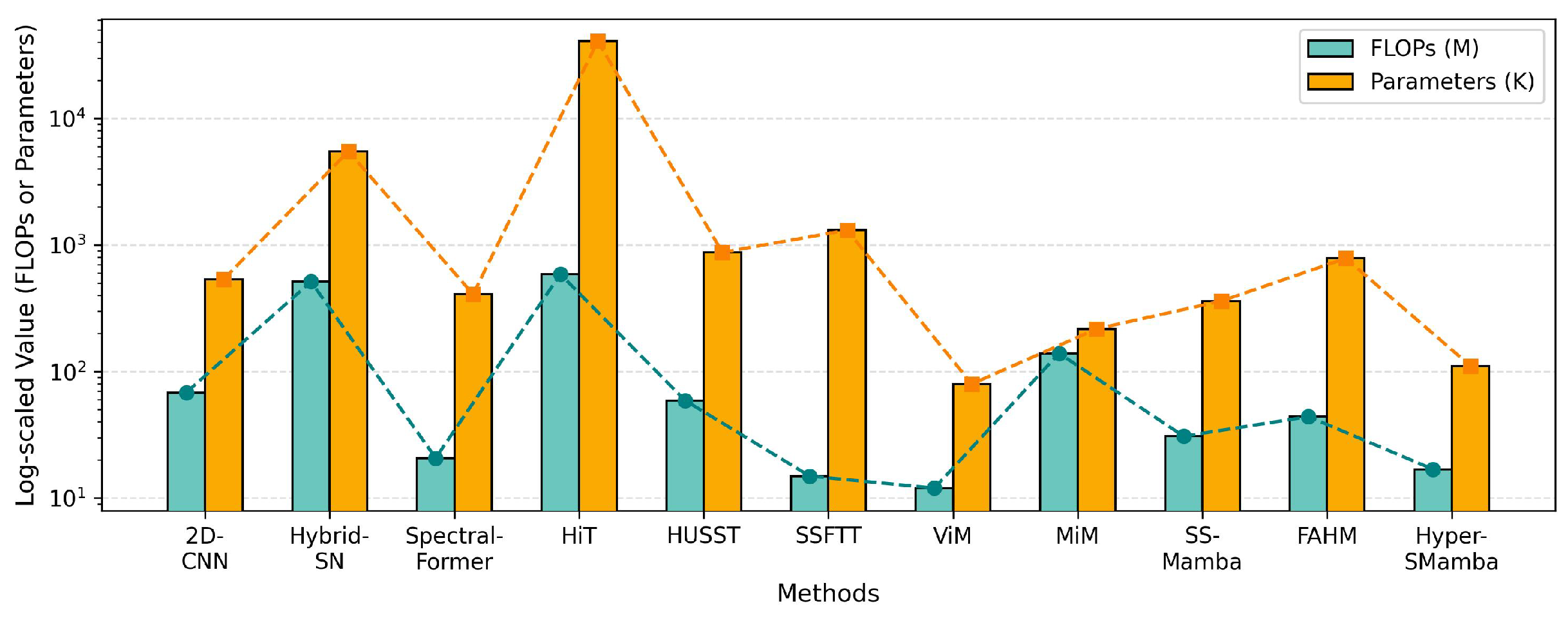
4.1. Discussion of the Computational Costs

To assess the computational efficiency of different methods, we calculated the number of parameters and Floating Point Operations (FLOPs) for each model on the IP dataset, and summarized the results in

Table 9. The number of parameters (K) and computational complexity (MFLOPs) of different comparison experiments on the IP dataset.

Methods	2D CNN	Hybrid-SN	Spectral-Former	HiT	SSFTT	HUSST	ViM	MiM	SS-Mamba	FAHM	Hyper-Mamba
FLOPs (M)	68.53	512.94	20.77	587.92	59.25	14.96	12.02	139.4	30.89	44.12	16.93
Parameters (K)	537.87	5490.43	407.96	40,670.19	875.22	1310.71	79.87	217.36	360.62	784.74	110.88

. In order to further visualize the differences in resource consumption, a combined bar and line chart is provided in Appendix A Figure A2. Tables and charts indicate significant differences across methods in terms of computational efficiency and parameter scale.

HybridSN employs local convolution computations, but its computational complexity and parameter count increase rapidly with larger patch sizes, limiting its applicability in high-resolution scenarios. While both Transformer-based and Mamba-based models can establish long-range dependencies, they exhibit notable differences in computational complexity and parameter scale. The Mamba-based model has superior computing efficiency. For instance, ViM achieves the lowest number of parameters and computational complexity, requiring only 79.87k parameters and 12.02M FLOPs. Similarly, the proposed HyperSMamba maintains strong classification performance with only 16.93M FLOPs, which is more than 90% lower than the computational costs of HiT and HybridSN.

Focusing on Mamba-based architectures, the proposed HyperSMamba model achieves the highest classification accuracy among its peers. It is noteworthy that HyperSMamba exhibits a substantial reduction in both computational complexity and parameter count compared with SS-Mamba, MiM, and FAHM. On the Indian Pines dataset, although it introduces a slight increase in computational cost and parameter usage relative to ViM, it achieves a 9.22% improvement in overall accuracy (OA), demonstrating an excellent trade-off between efficiency and classification performance. This favorable balance highlights HyperSMamba’s strong potential for practical and industrial deployment.

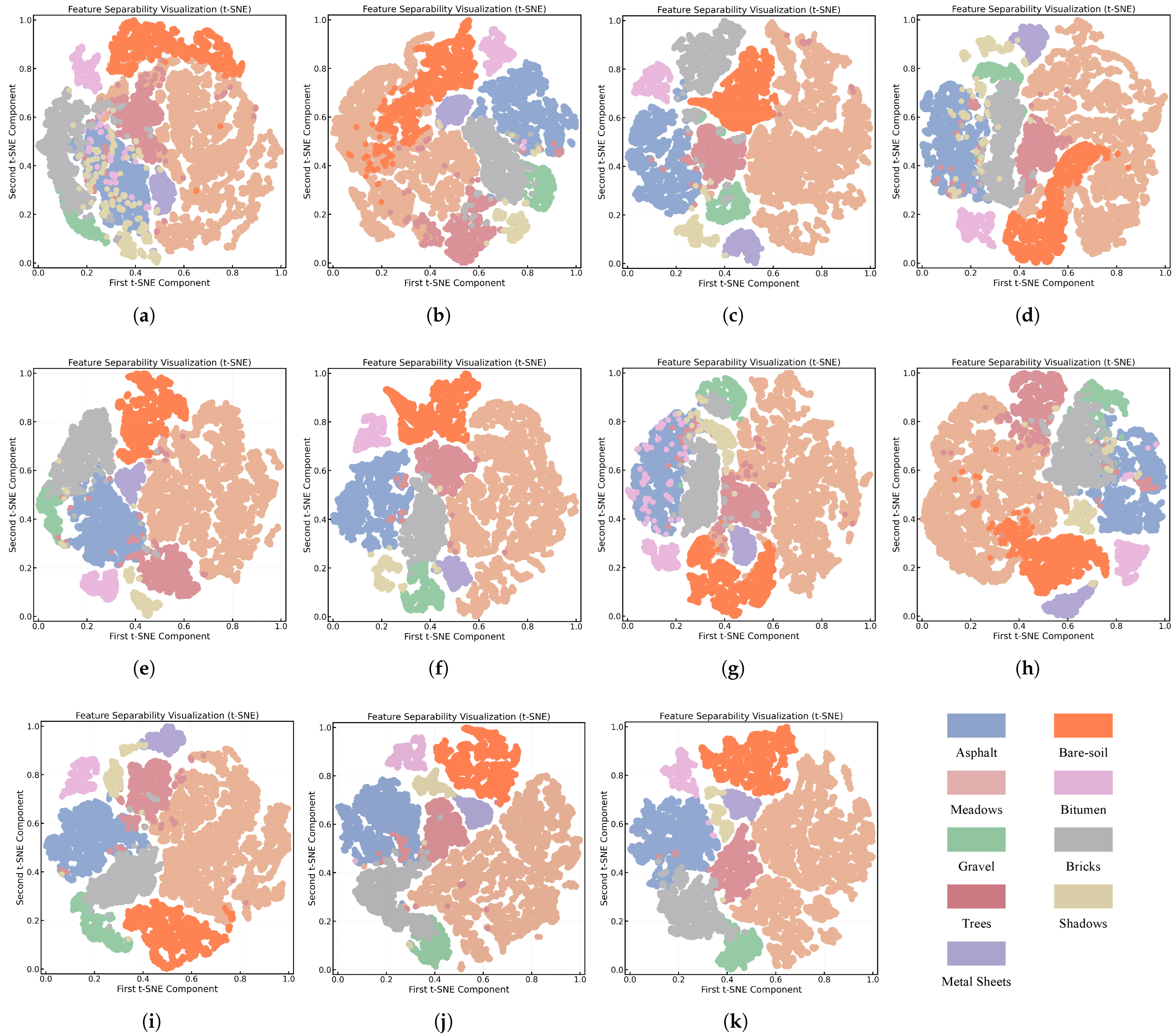
4.2. Learned Feature Visualizations by T-SNE

The high-dimensional features extracted by the model are mapped into a 2D space using t-Distributed Stochastic Neighbor Embedding (T-SNE) to intuitively assess the model’s feature extraction capability. The visualization outcomes of each comparative experiment on the UP dataset are shown in Figure 7. In the T-SNE plots, each point represents a pixel from the Pavia University test set, colored by its ground-truth class. The horizontal and vertical axes denote the first and second components of the t-SNE embedding, both normalized to the range $[0,1]$. Although these axes have no physical units, they reflect the relative positioning of feature representations in the projected space.

Specifically, the features of 2D-CNN and ViM are relatively scattered, and the class boundaries are unclear, reflecting the insufficient feature extraction capability of these models, which fail to adequately distinguish the feature representations of different classes in the high-dimensional feature space. Our method produces more compact and well-separated clusters, with clearer boundaries between categories after dimensionality reduction, indicating that the model has learned more discriminative features in the high-dimensional space. Furthermore, the proposed model exhibits smoother transitions between similar categories, reducing inter-class overlap by capturing subtle feature differences more precisely.

4.3. Parameters Analyzed

We explore the impact of two key hyperparameters, patch size and the number of bands after PCA processing, on the classification accuracy of HSI.

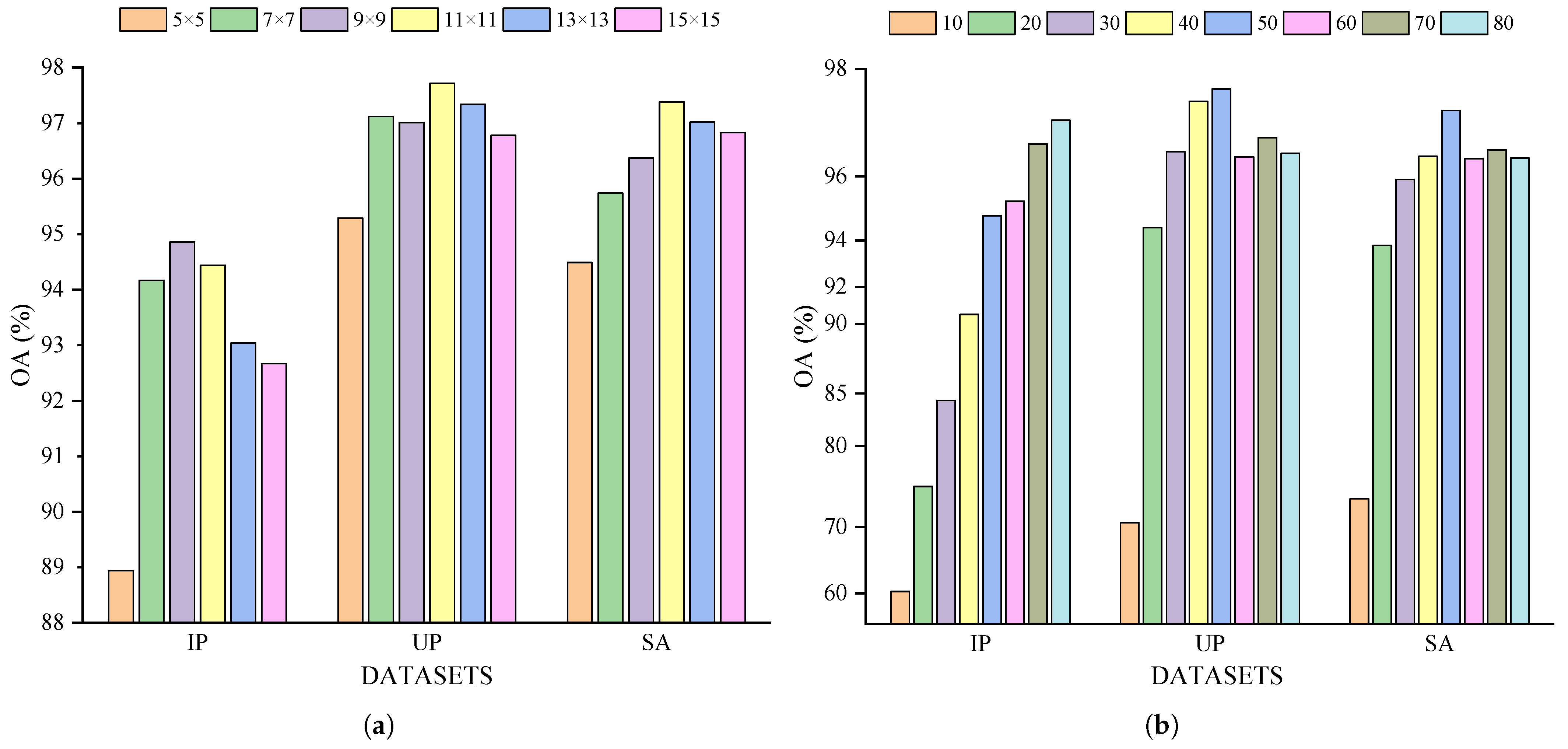
4.3.1. Impact of the Patch Size

In HSIC tasks, patch size directly influences the ability to extract spatial information. We calculated the classification accuracy for each dataset under different follow-up patch sizes.

As illustrated in Figure 8a, appropriately increasing patch size allows for the capture of more spatial contextual information while retaining local details. However, when the patch size becomes too large, the model may incorporate excessive background information, leading to information overlap between classes and consequently reducing classification accuracy, while significantly increasing computational cost. The IP dataset attained the maximum classification accuracy with a patch size of $9\times 9$, while the SA and UP datasets reached optimal performance with a patch size of $11\times 11$.

4.3.2. Impact of the Number of Bands After PCA

Principal component analysis (PCA) is used to retain key information while decreasing computational complexity. We tested the effect of different dimensions after PCA on classification performance, as shown in Figure 8b.

In the IP dataset, spectral differences between classes are subtle. Lower PCA dimensions result in significant information loss, making it difficult to effectively distinguish fine-grained classes and leading to significantly lower classification accuracy. As the number of retained components increases to 50, the OA rises sharply, primarily due to the enhanced discriminative capability resulting from the preservation of more critical spectral features. With further increases in dimensionality, the OA exhibits a further upward trend, indicating that high-dimensional representations are more beneficial for classifying the IP dataset. However, this also leads to a significant increase in model parameters, thereby introducing additional computational overhead. In contrast, the UP and SA datasets have higher spatial resolution and fewer spectral channels. When the PCA dimension is set to 10, there is considerable information loss, resulting in lower classification accuracy. However, OA reaches the maximum value when the PCA dimension is increased to 50. When the PCA dimension exceeds 50, excessive noise and redundant features are retained, which reduces classification accuracy and increases computational complexity.

4.4. Discussion of the Strengths and Limitations

The key to HSIC lies in the effective utilization of spectral and spatial features. Insufficient spatial information may lead to misclassification of land cover types that share similar spectral characteristics but differ in spatial distribution. Conversely, excessive spatial information without adequately leveraging spectral data may cause the model to overfit to local spatial patterns while neglecting the discriminative potential of spectral signatures. To improve the model’s capacity for establishing long-range dependencies in spectral and spatial dimensions while decreasing the number of parameters and computational expenses, we employed ViM as the base architecture. However, as shown in the comparative experiments in Table 4, Table 5 and Table 6, the inherent causal properties of SSM limit its ability to extract spatial features. Therefore, we designed a lightweight MSFM to extract features at multiple scales and used this module to integrate spatial state information, thereby enhancing the representation of local spatial features. The comparative results and classification maps clearly illustrate the benefits of HyperSMamba. In contrast to CNN-based models, HyperSMamba establishes long-range dependencies and improves the recognition accuracy of boundary pixels between classes. Although Transformer-based models (such as SpectralFormer and HiT) possess global modeling capabilities, their computational complexity is high, and they underutilize spatial information in small-scale regions, leading to misclassification of fine-grained categories. In contrast, HyperSMamba achieves higher classification accuracy while reducing computational overhead, particularly in areas where class boundaries are unclear and spectral similarity is high, exhibiting greater classification stability.

Despite the excellent performance of HyperSMamba in hyperspectral image classification tasks, the method still exhibits several potential limitations that warrant further investigation and improvement. One major issue is the class imbalance commonly observed in hyperspectral datasets, where certain classes contain relatively few and sparsely distributed samples. This often leads the model to focus on optimizing the classification accuracy for dominant classes, while overlooking underrepresented ones. Another limitation lies in the conversion of 2D spatial images into sequential inputs for the state-space mechanism (SSM). The current implementation employs simple horizontal or vertical scanning strategies, which may fail to capture more complex and semantically meaningful spatial dependencies.

To address these limitations, future work will focus on improving spectral feature extraction mechanisms, enabling the model to adaptively emphasize challenging categories during training. We also performed preliminary experiments to model spectral sequences directly using SSM, but the results were not promising. This finding suggests that introducing an effective feature extraction module before the SSM for refining and condensing spectral features could significantly enhance the model’s performance. Regarding spatial sequence construction, we plan to explore more expressive strategies, such as graph-based or tree-based transformations, to better preserve spatial structure and improve the representational capacity of the SSM module.

5. Conclusions

To further explore the application of Vision Mamba in hyperspectral imaging, we propose a hyperspectral classification framework, HyperSMamba. The model introduces a Multi-Scale State Fusion Module (MSFM) to enhance the recognition capability of features across multiple scales and integrate the spatial relationships of the state matrix in FusionSSM. Furthermore, the AFAttention module is employed to enhance and fuse spectral–spatial features, enabling the extraction of more discriminative information. Ablation studies demonstrate that the proposed MSFM and AFAttention are effective. The model achieves overall accuracies of 94.86%, 97.72%, and 97.38% on the IP, UP, and SA datasets, respectively. Both visual and quantitative analyses indicate that the model exhibits strong robustness and effectiveness in hyperspectral image classification tasks, fully leveraging features to improve classification accuracy. Although the model achieves excellent performance, it still faces several challenges, such as overcoming the limitations of causal properties of the state-space model, and further optimizing the feature representation capability of the Mamba architecture while maintaining high computational efficiency. These are key directions for our future research.

References

1. Li, D.; Wu, J.; Zhao, J.; Xu, H.; Bian, L. SpectraTrack: Megapixel, Hundred-fps, and Thousand-channel Hyperspectral Imaging. Nat. Commun. 2024, 15, 9459. [Google Scholar] [CrossRef] [PubMed]
2. Jia, J.W.; Wang, Y.H.; Chen, J.Y.; Guo, R.L.; Shu, R.M.; Wang, J.Q. Status and Application of Advanced Airborne Hyperspectral Imaging Technology: A Review. Infrared Phys. Technol. 2020, 104, 103115. [Google Scholar] [CrossRef]
3. Bhargava, A.; Sachdeva, A.; Sharma, K.; Alsharif, M.H.; Uthansakul, P.; Uthansakul, M. Hyperspectral imaging and its applications: A review. Heliyon 2024, 10, 33208. [Google Scholar] [CrossRef]
4. Ahmad, M.; Shabbir, S.; Roy, S.K.; Hong, D.; Wu, X.; Yao, J. Hyperspectral Image Classification—Traditional to Deep Models: A Survey for Future Prospects. IEEE J. Sel. Top. Appl. Earth Obs. Remote Sens. 2022, 15, 968–999. [Google Scholar] [CrossRef]
5. Zhang, W.; Zhao, L. The Track, Hotspot and Frontier of International Hyperspectral Remote Sensing Research 2009–2019—A Bibliometric Analysis Based on SCI Database. Measurement 2022, 187, 110229. [Google Scholar] [CrossRef]
6. Ma, X.; Wang, H.; Geng, J. Spectral–spatial Classification of Hyperspectral Image Based on Deep Auto-encoder. IEEE J. Sel. Top. Appl. Earth Obs. Remote Sens. 2016, 9, 4073–4085. [Google Scholar] [CrossRef]
7. Hu, W.; Huang, Y.; Wei, L.; Zhang, F.; Li, H. Deep Convolutional Neural Networks for Hyperspectral Image Classification. J. Sens. 2015, 2015, 258619. [Google Scholar] [CrossRef]
8. Ding, Y.; Zhang, Z.; Zhao, X.; Hong, D.; Cai, W.; Yu, C.; Yang, N.; Cai, W. Multi-feature Fusion: Graph Neural Network and CNN Combining for Hyperspectral Image Classification. Neurocomputing 2022, 501, 246–257. [Google Scholar] [CrossRef]
9. Song, T.; Wang, Y.; Gao, C.; Chen, H.; Li, J. MSLAN: A Two-branch Multi-directional Spectral–Spatial LSTM Attention Network for Hyperspectral Image Classification. IEEE Trans. Geosci. Remote Sens. 2022, 60, 5528814. [Google Scholar] [CrossRef]
10. Mou, L.; Ghamisi, P.; Zhu, X.X. Deep Recurrent Neural Networks for Hyperspectral Image Classification. IEEE Trans. Geosci. Remote Sens. 2017, 55, 3639–3655. [Google Scholar] [CrossRef]
11. Mei, S.; Song, C.; Ma, M.; Xu, F. Hyperspectral Image Classification Using Group-Aware Hierarchical Transformer. IEEE Trans. Geosci. Remote Sens. 2022, 60, 1–14. [Google Scholar] [CrossRef]
12. Krizhevsky, A.; Sutskever, I.; Hinton, G.E. ImageNet Classification with Deep Convolutional Neural Networks. Commun. ACM 2017, 60, 84–90. [Google Scholar] [CrossRef]
13. Chollet, F. Xception: Deep Learning with Depthwise Separable Convolutions. In Proceedings of the 2017 IEEE Conference on Computer Vision and Pattern Recognition, Honolulu, HI, USA, 21–26 July 2017. [Google Scholar] [CrossRef]
14. Li, Y.; Zhang, H.; Shen, Q. Spectral–Spatial Classification of Hyperspectral Imagery with 3D Convolutional Neural Network. Remote Sens. 2017, 9, 67. [Google Scholar] [CrossRef]
15. Zhou, J.; Zeng, S.; Xiao, Z.; Zhou, J.; Li, H.; Kang, Z. An Enhanced Spectral Fusion 3D CNN Model for Hyperspectral Image Classification. Remote Sens. 2022, 14, 5334. [Google Scholar] [CrossRef]
16. Xu, Z.; Su, C.; Wang, S.; Zhang, X. Local and Global Spectral Features for Hyperspectral Image Classification. Remote Sens. 2023, 15, 1803. [Google Scholar] [CrossRef]
17. Roy, S.K.; Krishna, G.; Dubey, S.R.; Chaudhuri, B.B. HybridSN: Exploring 3D-2D CNN Feature Hierarchy for Hyperspectral Image Classification. IEEE Geosci. Remote Sens. Lett. 2020, 17, 277–281. [Google Scholar] [CrossRef]
18. Chen, J.; Wang, X.J.; Guo, Z.C.; Zhang, X.Y.; Sun, J. Dynamic Region-aware Convolution. In Proceedings of the 2021 IEEE/CVF Conference on Computer Vision and Pattern Recognition, Nashville, TN, USA, 20–25 June 2021. [Google Scholar] [CrossRef]
19. Hong, D.; Han, Z.; Yao, J.; Gao, L.; Zhang, B.; Plaza, A.; Chanussot, J. SpectralFormer: Rethinking Hyperspectral Image Classification with Transformers. IEEE Trans. Geosci. Remote Sens. 2022, 60, 1–15. [Google Scholar] [CrossRef]
20. Zhao, Z.; Hu, D.; Wang, H.; Yu, X. Convolutional Transformer Network for Hyperspectral Image Classification. IEEE Geosci. Remote Sens. Lett. 2022, 19, 1–5. [Google Scholar] [CrossRef]
21. He, X.; Chen, Y.; Lin, Z. Spatial-spectral Transformer for Hyperspectral Image Classification. Remote Sens. 2021, 13, 498. [Google Scholar] [CrossRef]
22. Ma, C.; Jiang, J.; Li, H.; Mei, X.; Bai, C. Hyperspectral Image Classification Via Spectral Pooling and Hybrid Transformer. Remote Sens. 2022, 14, 4732. [Google Scholar] [CrossRef]
23. Sun, L.; Zhao, G.; Zheng, Y.; Wu, Z. Spectral–Spatial Feature Tokenization Transformer for Hyperspectral Image Classification. IEEE Trans. Geosci. Remote Sens. 2022, 60, 1–14. [Google Scholar] [CrossRef]
24. Yang, X.; Cao, W.; Lu, Y.; Zhou, Y. Hyperspectral Image Transformer Classification Networks. IEEE Trans. Geosci. Remote Sens. 2022, 60, 1–15. [Google Scholar] [CrossRef]
25. Zhou, W.; Kamata, S.I.; Luo, Z.; Chen, X. Hierarchical Unified Spectral-Spatial Aggregated Transformer for Hyperspectral Image Classification. In Proceedings of the 2022 26th International Conference on Pattern Recognition (ICPR), Montreal, QC, Canada, 21–25 August 2022. [Google Scholar] [CrossRef]
26. Gu, A.; Goel, K.; Ré, C. Efficiently Modeling Long Sequences with Structured State Spaces. arXiv 2021, arXiv:2111.00396. [Google Scholar] [CrossRef]
27. Gu, A.; Dao, T. Mamba: Linear-time Sequence Modeling with Selective State Spaces. arXiv 2023, arXiv:2312.00752. [Google Scholar] [CrossRef]
28. Zhu, L.; Liao, B.; Zhang, Q.; Wang, X.; Liu, W.; Wang, X. Vision Mamba: Efficient Visual Representation Learning with Bidirectional State Space Model. arXiv 2024, arXiv:2401.09417. [Google Scholar] [CrossRef]
29. Liu, Y.; Tian, Y.; Zhao, Y.; Yu, H.; Xie, L.; Wang, Y.; Ye, Q.; Jiao, J.; Liu, Y. Vmamba: Visual State Space Model. arXiv 2024, arXiv:2401.10166. [Google Scholar] [CrossRef]
30. Pei, X.; Huang, T.; Xu, C. Efficientvmamba: Atrous Selective Scan for Lightweight Visual Mamba. arXiv 2024, arXiv:2403.09977. [Google Scholar] [CrossRef]
31. Huang, T.; Pei, X.; You, S.; Wang, F.; Qian, C.; Xu, C. Localmamba: Visual State Space Model with Windowed Selective Scan. arXiv 2024, arXiv:2403.09338. [Google Scholar] [CrossRef]
32. Yao, J.; Hong, D.; Li, C.; Chanussot, J. Spectralmamba: Efficient Mamba for Hyperspectral Image Classification. arXiv 2024, arXiv:2404.08489. [Google Scholar] [CrossRef]
33. Yang, J.X.; Zhou, J.; Wang, J.; Tian, H.; Liew, A.W.C. Hsimamba: Hyperspectral Imaging Efficient Feature Learning with Bidirectional State Space for Classification. arXiv 2024, arXiv:2404.00272. [Google Scholar] [CrossRef]
34. Chen, K.; Chen, B.; Liu, C.; Li, W.; Zou, Z.; Shi, Z. Rsmamba: Remote Sensing Image Classification with State Space Model. arXiv 2024, arXiv:2403.19654. [Google Scholar] [CrossRef]
35. Zhuang, P.; Zhang, X.; Wang, H.; Zhang, T.; Liu, L.; Li, J. FAHM: Frequency-Aware Hierarchical Mamba for Hyperspectral Image Classification. IEEE J. Sel. Top. Appl. Earth Obs. Remote Sens. 2025, 18, 6299. [Google Scholar] [CrossRef]
36. Zhou, W.; Kamata, S.I.; Wang, H.; Wong, M.S.; Hou, H.C. Mamba-in-Mamba: Centralized Mamba-Cross-Scan in Tokenized Mamba Model for Hyperspectral Image Classification. Neurocomputing 2025, 613, 128751. [Google Scholar] [CrossRef]
37. Huang, L.; Chen, Y.; He, X. Spectral-Spatial Mamba for Hyperspectral Image Classification. Remote Sens. 2024, 16, 2449. [Google Scholar] [CrossRef]
38. Liu, X.; Zhang, C.; Zhang, L. Vision Mamba: A Comprehensive Survey and Taxonomy. arXiv 2024, arXiv:2405.04404. [Google Scholar] [CrossRef]
39. Xu, R.; Yang, S.; Wang, Y.; Cai, Y.; Du, B.; Chen, H. Visual Mamba: A Survey and New Outlooks. arXiv 2024, arXiv:2404.18861. [Google Scholar] [CrossRef]
40. Ma, P.; Ren, J.; Zhao, H.; Sun, G.; Murray, P.; Zheng, J. Multiscale 2-D Singular Spectrum Analysis and Principal Component Analysis for Spatial-Spectral Noise-robust Feature Extraction and Classification of Hyperspectral Images. IEEE J. Sel. Top. Appl. Earth Obs. Remote Sens. 2021, 14, 1233–1245. [Google Scholar] [CrossRef]
41. Yang, A.; Li, M.; Ding, Y.; Hong, D.; Lv, Y.; He, Y. GTFN: GCN and Transformer Fusion Network with Spatial-Spectral Features for Hyperspectral Image Classification. IEEE Trans. Geosci. Remote Sens. 2023, 61, 1–15. [Google Scholar] [CrossRef]
42. Dao, T.; Gu, A. Transformers Are SSMs: Generalized Models and Efficient Algorithms Through Structured State Space Duality. arXiv 2024, arXiv:2405.21060. [Google Scholar] [CrossRef]
43. Gu, A.; Johnson, I.; Goel, K.; Saab, K.; Dao, T.; Rudra, A. Combining Recurrent, Convolutional, and Continuous-Time Models with Linear State Space Layers. In Proceedings of the Advances in Neural Information Processing Systems (NeurIPS), San Diego, CA, USA, 6–14 December 2021. [Google Scholar]
44. Piqueras, S.; Burger, J.; Tauler, R.; de Juan, A. Relevant Aspects of Quantification and Sample Heterogeneity in Hyperspectral Image Resolution. Chemom. Intell. Lab. Syst. 2012, 117, 169–182. [Google Scholar] [CrossRef]
45. Zhang, X.; Zhou, X.; Lin, M.; Sun, J. Shufflenet: An Extremely Efficient Convolutional Neural Network for Mobile Devices. In Proceedings of the IEEE Conference on Computer Vision and Pattern Recognition, Salt Lake City, UT, USA, 18–23 June 2018. [Google Scholar] [CrossRef]
46. Zhu, X.; Cheng, D.; Zhang, Z.; Lin, S.; Dai, J. An Empirical Study of Spatial Attention Mechanisms in Deep Networks. In Proceedings of the 2019 IEEE/CVF International Conference on Computer Vision (ICCV), Seoul, Republic of Korea, 27 October–2 November 2019. [Google Scholar] [CrossRef]
Figure 1. The overall architecture of HyperSMamba.
Remotesensing 17 02008 g001
Figure 2. Illustration of the Multi-Scale State Fusion module.
Remotesensing 17 02008 g002
Figure 3. (a) The structure of the Adaptive Fusion Attention Module, which comprises the following three components: (b) spatial attention; (c) pixel attention; (d) channel attention.
Remotesensing 17 02008 g003
Figure 4. Land cover maps of all comparative experiments on the Indian Pines dataset: (a) ground truth, (b) 2D CNN, (c) HybridSN, (d) SpectralFormer, (e) HiT, (f) HUSST, (g) SSFTT, (h) ViM, (i) MiM, (j) SS-Mamba, (k) FAHM, (l) HyperSMamba.
Remotesensing 17 02008 g004
Figure 5. Land cover maps of all comparative experiments on the Pavia University dataset: (a) ground truth, (b) 2D CNN, (c) HybridSN, (d) SpectralFormer, (e) HiT, (f) HUSST, (g) SSFTT, (h) ViM, (i) MiM, (j) SS-Mamba, (k) FAHM, (l) HyperSMamba.
Remotesensing 17 02008 g005
Figure 6. Land cover maps of all comparative experiments on the Salinas dataset: (a) ground truth, (b) 2D CNN, (c) HybridSN, (d) SpectralFormer, (e) HiT, (f) HUSST, (g) SSFTT, (h) ViM, (i) MiM, (j) SS-Mamba, (k) FAHM, (l) HyperSMamba.
Remotesensing 17 02008 g006
Figure 7. Visualization of T-SNE results on the Pavia University dataset. (a) 2D CNN, (b) HybridSN, (c) SpectralFormer, (d) HiT, (e) HUSST, (f) SSFTT, (g) ViM, (h) MiM, (i) SS-Mamba, (j) FAHM, (k) HyperSMamba.
Remotesensing 17 02008 g007
Figure 8. Impacts of the different parameters on overall accuracy (OA) for three datasets: (a) Impact of the patch size. (b) Impact of the number of retained bands after PCA.
Remotesensing 17 02008 g008