A Lightweight Remote-Sensing Image-Change Detection Algorithm Based on Asymmetric Convolution and Attention Coupling

Abstract

Remote-sensing image-change detection is indispensable for land management, environmental monitoring and related applications. In recent years, breakthroughs in satellite sensor technology have generated vast volumes of data and complex scenes, presenting significant challenges for change-detection algorithms. Traditional methods rely on handcrafted features, which struggle to address the impacts of multi-source data heterogeneity and imaging condition differences. In this context, technology based on deep learning has made substantial breakthroughs in change-detection performance by automatically extracting high-level feature representations of the data. However, although the existing deep-learning models improve the detection accuracy through end-to-end learning, their high parameter count and computational inefficiency hinder suitability for real-time monitoring and edge device deployment. Therefore, to address the need for lightweight solutions in scenarios with limited computing resources, this paper proposes an attention-based lightweight remote sensing change detection network (ABLRCNet), which achieves a balance between computational efficiency and detection accuracy by using lightweight residual convolution blocks (LRCBs), multi-scale spatial-attention modules (MSAMs) and feature-difference enhancement modules (FDEMs). The experimental results demonstrate that the ABLRCNet achieves excellent performance on three datasets, significantly enhancing both the accuracy and robustness of change detection, while exhibiting efficient detection capabilities in resource-limited scenarios.

1. Introduction

Remote-sensing image-change detection is a core technology in the field of earth observation. It compares multi-temporal remote-sensing images of the same geographical area to perform pixel-level binary classification of time-series changes of land surface objects (0 indicates no change, 1 indicates change), aiming to identify land feature changes caused by urban expansion, deforestation and other activities, while suppressing background disturbances caused by seasonal fluctuations or atmospheric conditions. In recent years, the “three highs” of remote-sensing technology (high spatial resolution, high spectral resolution, and high temporal resolution) [1] have facilitated the acquisition of high-resolution images that not only expand the application scenarios of change detection (such as land management [2,3], urban planning [4,5], environmental monitoring [6,7,8] and disaster prediction [9]), but also imposes higher demands on the accuracy and efficiency of detection algorithms.

Traditional change detection methods are mainly divided into two types: pixel-level and object-level. Pixel-level methods (such as the difference method [10], the ratio method [11] and the spectral angle mapping method [12]) detect changes by calculating the spectral differences of multiple phases on a pixel-by-pixel basis and setting thresholds. In high-resolution scenarios, the spectral variation of similar ground objects can also lead to false detection and missed detection [13]. In order to overcome the above shortcomings, the object-level method divides the image into semantic homogeneity regions (i.e., “image objects”) through image segmentation and analyzes the changes based on the characteristics of the regions [14]. For example, the pixel–object–level fusion algorithm proposed by Su et al. [15] extracts the artificial feature-change region through sliding window segmentation and supervised classification, which effectively suppresses the salt-and-pepper noise, but the insufficient spatiotemporal consistency of the segmentation results may lead to detection errors. The conditional hybrid Markov model of Benedek et al. [16] improves the segmentation accuracy by fusing local correlation and global intensity features, but its performance remains constrained by the representational limitations of handcrafted features [17]. Although the object-level method improves the detection robustness through spatial information integration, the feature generalization ability and computational efficiency in complex scenes still need to be optimized [18].

Deep-learning technology overcomes the limitations of traditional methods through end-to-end feature learning. Early CNN models, such as the texture-aware network proposed by Ding et al. [19], have improved the accuracy of landslide detection by automatically extracting spectra–spatial features. Hou et al. [20], based on VGGNet’s hypercolumn feature-fusion method enhanced the ability to distinguish changes in complex backgrounds through multi-level semantic information extraction. In recent years, the research on deep learning in change detection has advanced significantly across several fronts:

(1)

The Siamese network and attention mechanism: The twin CNN of Zhan et al. [21] learned the similarities and differences between cells through weighted contrast loss and performed well in aerial image detection. The multi-path attention residual block proposed by Zhang et al. [22] realizes the differentiated processing of multi-scale features through the channel-attention mechanism, and effectively copes with the interference of light changes and vegetation seasons.

(2)

Multimodal and multi-scale fusion: Wang et al. [23] improved the registration accuracy of hyperspectral images by generating hybrid affine matrices. The spectral–spatial joint learning network of Zhang et al. [24] synchronously extracts multi-dimensional features through the twin structure, which significantly enhances the representation ability of change information.

(3)

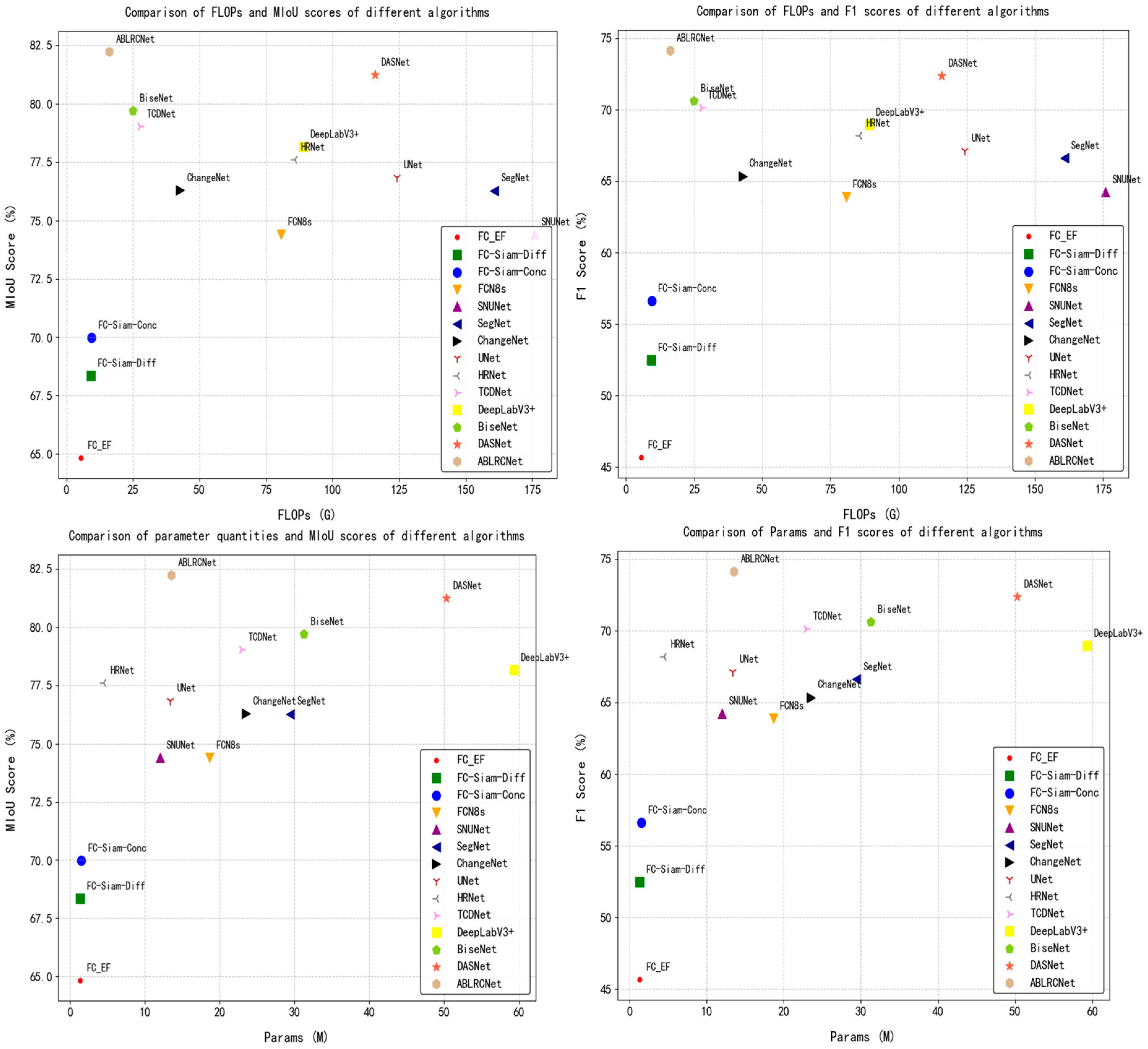
Lightweight and edge deployment: Although deep models significantly improve detection accuracy, the high computational complexity of mainstream methods (such as SNUNet, 175.76 G FLOPs) limits their application in resource-constrained scenarios such as drones and edge devices. Lightweight designs such as the MobileNet variant [25] reduce the amount of computation, but the accuracy of small target detection is reduced due to an insufficient receptive field [26].

The existing methods face a dual challenge in the “precision–efficiency” balance: traditional methods struggle with the complex features of high-resolution images, while deep-learning models generally suffer from the problems of parameter redundancy and high computational cost. To address this challenge, this paper proposes a lightweight network based on asymmetric convolution and attention coupling, ABLRCNet, and its core innovations include:

• The introduction of lightweight residual convolution blocks reduces parameter complexity and computational complexity, while ensuring the effective extraction and transfer of features, which significantly compresses the calculation cost of the model.
• The multi-scale spatial-attention module enables the network to pay attention to features of different scales, enhancing its ability to capture change information from objects of varying sizes in remote sensing imagery.
• The proposed feature difference enhancement module further highlights the features of the changed regions through the enhanced processing of feature differences of remote-sensing images at distinct phases, leading to more accurate localization and identification of the changed regions.
• Quantitative and qualitative experiments on three datasets demonstrate that our proposed ABLRCNet effectively balances computational resources and detection accuracy.

The remainder of the paper is divided into the following sections: Section 2 begins with a detailed description of the composition and selection advantages of each module of the network model, followed by the introduction and analysis of three experimental datasets, namely the BTCDD, LEVIR-CD and BCDD datasets. Section 3 first performed two ablation experiments on the BTCDD dataset, followed by experiments to demonstrate the performance of the model on three datasets. Section 4 discusses proposed modules and future prospects.

2. Methodology and Materials

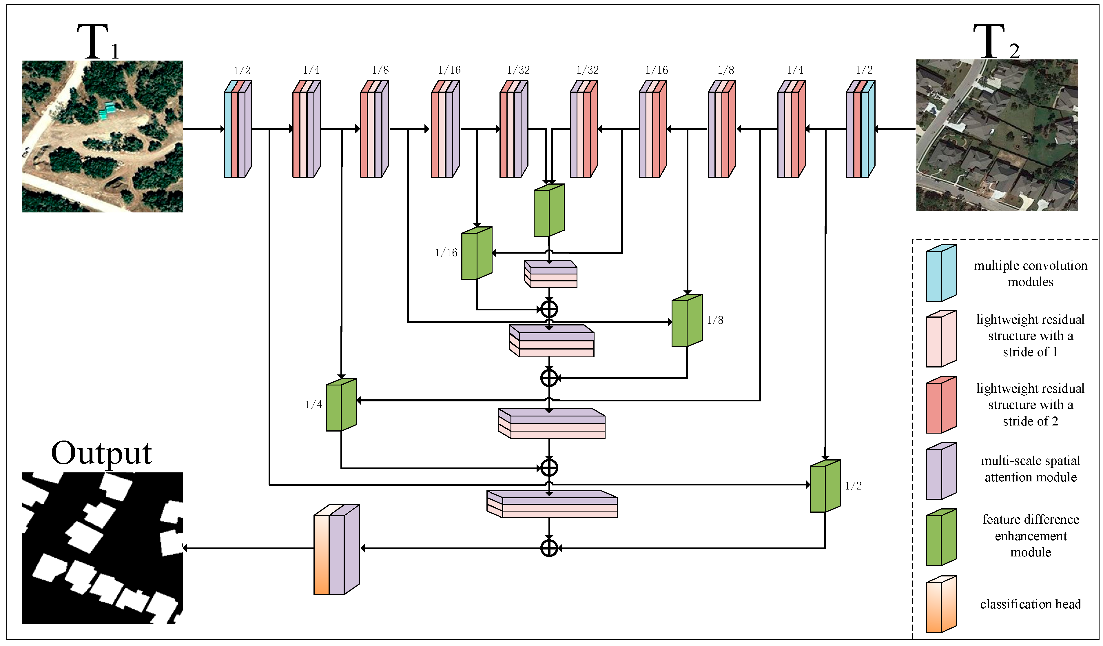
2.1. Network Architecture

In the field of remote-sensing image-change detection, lightweight and accurate methods have been central to research. The lightweight attention-based remote-sensing change-detection network (ABLRCNet) proposed here aims to solve problems that traditional methods struggle to balance between computational resources and detection accuracy.

The proposed network model is depicted in Figure 1. It adopts an encoder–decoder architecture, incorporating lightweight residual convolution blocks. This module can ensure effective feature extraction and transmission while reducing parameter complexity and computational complexity, thus significantly reducing the calculation cost of the model. The multi-scale spatial-attention module enables ABLRCNet to focus on different scale features, enhancing its ability to capture the change information of different size elements in remote-sensing images. The feature-difference enhancement module further amplifies features of the changed regions through the enhanced processing of feature differences between remote sensing images at multiple phases, facilitating more precise localization and identification of changing regions.

Table 1. Basic network structure parameters of ABLRCNet. Here, [3 × 3, 32] denotes a 3 × 3 convolution with 32 output channels, and [LRCB, 32, 2] represents a lightweight residual convolutional block with 32 output channels and a stride of 2.

—	Stage	Output Size	Network 1	Network 2	—	Stage	Output Size	—
Encoder	D1	1/2	[3 × 3, 32] × 3 [LRCB, 32, 2] [MSAM]	Weight Sharing	Decoder	U1	1/16	[MSAM] [LRCB, 256, 1] [LRCB, 256, 1]
	D2	1/4	[LRCB, 64, 2] [LRCB, 64, 1] [MSAM]			U2	1/8	[MSAM] [LRCB, 128, 1] [LRCB, 128, 1]
	D3	1/8	[LRCB, 128, 2] [LRCB, 128, 1] [MSAM]			U3	1/4	[MSAM] [LRCB, 64, 1] [LRCB, 64, 1]
	D4	1/16	[LRCB, 256, 2] [LRCB, 256, 1] [MSAM]			U4	1/2	[MSAM] [LRCB, 32, 1] [LRCB, 32, 1]
	D5	1/32	[LRCB, 512, 2] [LRCB, 512, 1] [MSAM]			Prediction	1	[MSAM] [1 × 1, 2] [Upsample]

describes the basic network structure parameters of ABLRCNet. The encoder stage of feature extraction is composed of multiple lightweight residual convolution blocks and multi-scale spatial-attention modules. The lightweight residual convolution blocks are responsible for extracting feature information of different scales, which provides the basis for subsequent processing. By integrating multi-scale spatial information, the multi-scale spatial-attention module enhances the spatial expression ability of features so that the network can focus more on the changed region. Each block is downsampled by D stages (D1, D2, D3, D4, D5) to reduce the image resolution. The resolution of each layer is 1/2, 1/4, 1/8, 1/16, and 1/32 of the original image size, respectively, and the number of input feature channels for each layer is 32, 64, 128, 256, and 512, respectively. Then, the feature-difference enhancement module further improves the expression ability of the features by capturing the differences and similarities between features, thereby improving the overall detection performance. The feature-fusion decoder of the model is also composed of multiple lightweight residual convolution blocks and multi-scale spatial-attention modules. The edge details of the feature map are gradually recovered by upsampling U stages (U1, U2, U3, U4) layer by layer, and subsequently the change feature map of the image is generated through using the classification head.

To address the computational efficiency and multi-scale feature-learning challenges, the proposed ABLRCNet adopts an encoder–decoder framework integrated with three key modules: lightweight residual convolution blocks (LRCBs), multi-scale spatial-attention modules (MSAMs), and feature-difference enhancement modules (FDEMs). The following subsections detail their designs and synergistic roles.

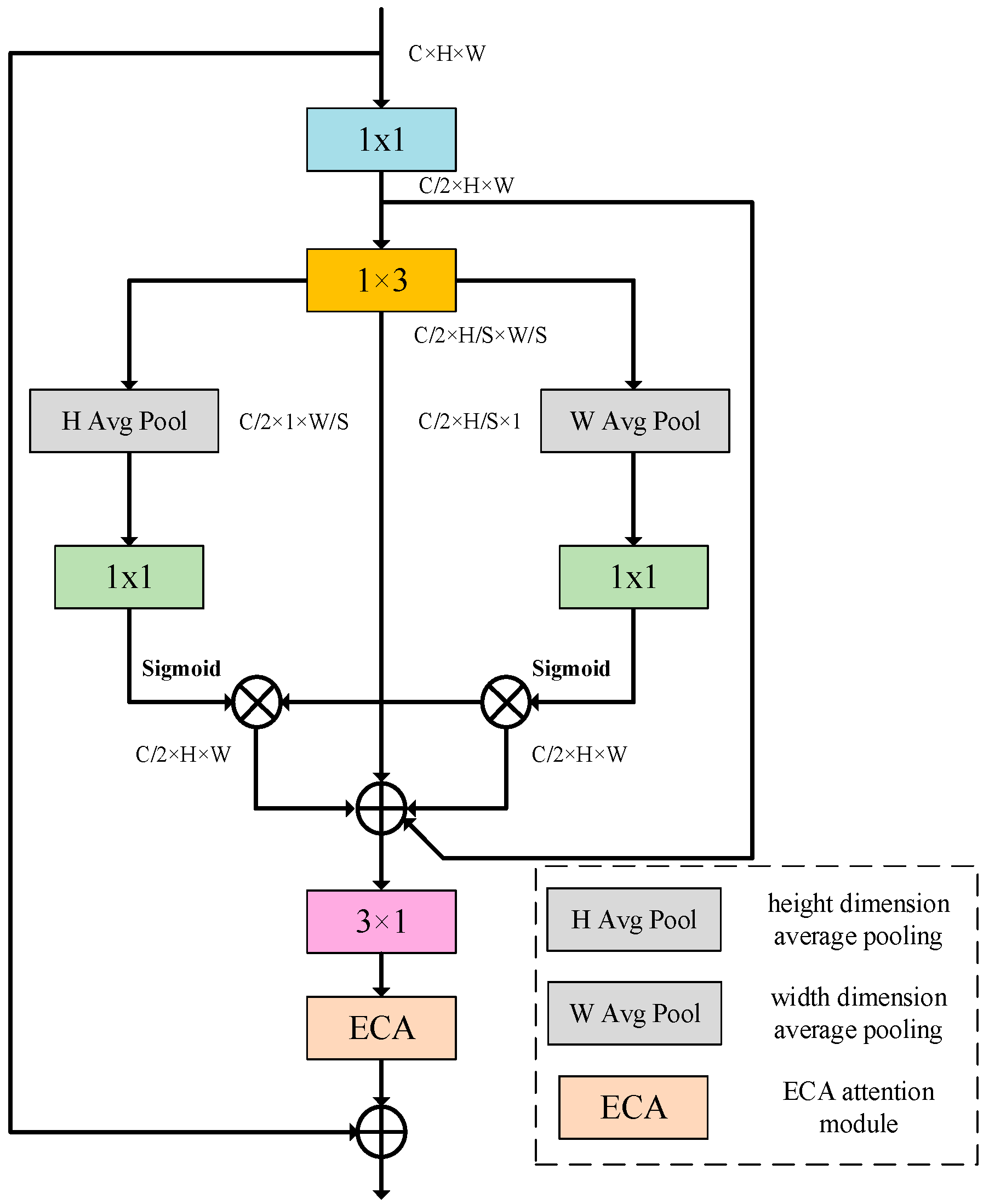
2.2. Lightweight Residual Convolution Blocks (LRCBs)

Lightweight residual convolutional blocks (LRCBs), as the core component of the backbone network, are inspired by the extreme pursuit of computational efficiency and feature extraction in deep learning. In practical application scenarios, especially when processing large-scale remote-sensing images, the traditional convolutional blocks expose many problems. Given the large amount of remote-sensing image data and high resolution, the large amount of computing resources required by traditional convolutional blocks become a bottleneck that hinders efficient processing, which not only consumes long time and hardware resources, but also leads to difficulty in deploying the model on resource-limited devices [27]. The LRCB constructed in this work not only reduces the computational cost, but also ensures the effectiveness of feature extraction, which provides a feasible scheme to solve the above problems.

The LRCB mainly comprises multiple convolution layers, a batch normalization (BN) layer, an activation function (ReLU), an adaptive average pooling layer, an ECA (efficient channel attention) module and a residual connection, as shown in Figure 2. First, $1\times 1$ convolution is applied to compress channel dimensionality in the input feature map by half. This dimensionality reduction significantly lowers the amount of computation for subsequent convolutional layers and also helps to remove redundant information in feature graphs and improve computational efficiency. Then, the spatial feature extraction is carried out by using $1\times 3$ and $3\times 1$ convolution kernels. This asymmetric convolution method can capture local feature information in different directions. In the horizontal direction, the $1\times 3$ convolution kernel extracts local feature information in the horizontal direction, such as horizontal edges and lines in the image. In the vertical direction, the $3\times 1$ convolution kernel focuses on extracting local features in the vertical direction, such as vertical edges, textures, etc. Through this approach, the local feature information can be captured in different directions, and the spatial local feature of the image can be modeled more comprehensively. Meanwhile, compared with $3\times 3$ traditional convolution, this separation convolution method significantly compresses the model’s parameter scale, the computational load and memory consumption [28]. In addition, horizontal-adaptive average pooling and vertical-adaptive average pooling are introduced to enhance the representation of the network. The horizontal-adaptive average pooling compresses the feature map to 1 in the height direction, while the width direction remains unchanged. In this way, it can aggregate information on the horizontal direction of the feature graph to obtain global statistics on the horizontal direction of each channel. The vertical-adaptive pooling compresses the feature map to 1 in the width direction, leaving the height direction unchanged. In this way, the vertical information of the feature map is aggregated and the global statistics of each channel in the vertical direction can be obtained. Then, the feature map after recovering the number of channels is further enhanced by an ECA module. The ECA module adaptively adjusts the weights between channels. It learns the importance weight of each channel through the local cross-channel interaction of the features in the channel dimension, and then reweights the features of different channels. Finally, the input feature map is added to the output feature map after a series of operations, which builds a direct connection path from the input to the output, that is, residual connection. The residual connection can effectively mitigate vanishing gradients problem with network deepening. Mathematical expressions of above processes are as follows:

$$f_{in}^{\prime }=f^{1\times 1}\left(f_{in}\right),$$

(1)

$$f_{in}^{″}=f^{1\times 3}\left(f_{in}^{\prime }\right),$$

(2)

$$f_H=f_{in}^{″}\otimes \sigma \left(f_{•}^{1\times 1}\left(GA{P}_H\left(f_{in}^{″}\right)\right)\right),$$

(3)

$$f_W=f_{in}^{″}\otimes \sigma \left(f_{•}^{1\times 1}\left(GA{P}_W\left(f_{in}^{″}\right)\right)\right),$$

(4)

$$f_{out}=f_{in}+ECA\left(f^{3\times 1}\left(f_{in}^{″}+f_H+f_W+f_{in}^{\prime }\right)\right),$$

(5)

where $f_{in}$ is the input feature map; $f_{in}^{,}$ is the output after 1 × 1 convolution for channel reduction (halving the channel dimension from C to C/2″); ${\mathrm{f}}^{1\times 1}\left(\cdot \right)$ denotes the two-dimensional 1 × 1 convolution; ${\mathrm{f}}^{1\times 3}\left(\cdot \right)$ denotes the two-dimensional 1 × 3 convolution; $\mathrm{G}\mathrm{A}{\mathrm{P}}_{\mathrm{H}}\left(\cdot \right)$ denotes the H-dimensional average pooling; $GA{P}_W\left(\cdot \right)$ denotes the W-dimensional average pooling; $f_{•}^{1\times 1}\left(\cdot \right)$ denotes the two-dimensional convolution with a convolution kernel of 1, with batch normalization; $\sigma \left(\cdot \right)$ represents a Sigmoid activation function; $\otimes$ denotes a matrix multiplication operation; $f^{3\times 1}\left(\cdot \right)$ denotes two-dimensional convolution with convolution kernel (3, 1), including batch normalization and an ReLU activation function and $ECA\left(\cdot \right)$ denotes the ECA channel attention operation.

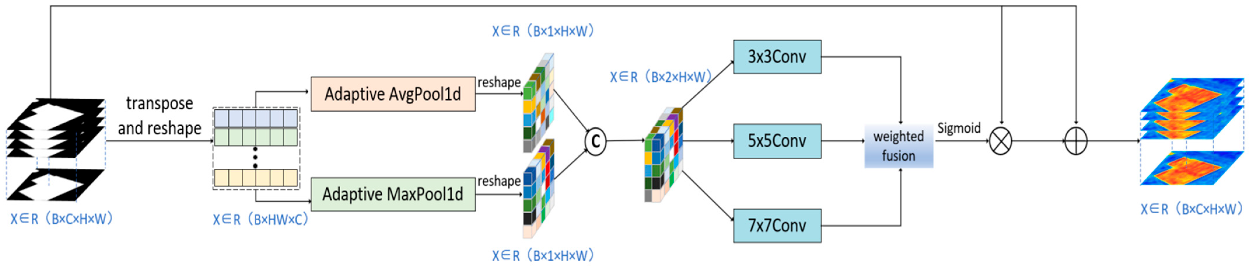
2.3. Multi-Scale Spatial-Attention Module (MSAM)

Multi-scale spatial information can provide a more comprehensive perspective for the model, small-scale information can help accurately locate subtle change details, and large-scale information can grasp the overall change trend. By fusing spatial information of different scales, the model can more accurately identify and distinguish the change regions of various sizes, which significantly improves the accuracy and reliability of change detection in remote-sensing images [29]. In this section, a multi-scale spatial-attention module (MSAM) is proposed, which is designed to enhance the model’s collaborative perception of local details and global semantics by fusing attention maps of different receptive fields with different convolutional kernel sizes k (=3, 5, 7), so as to enhance the model’s perception of objects and features of different sizes. The design of the multi-scale convolutional kernel is inspired by the idea of multi-resolution in time-frequency analysis, which is similar to wavelet analysis to decompose the time-frequency characteristics of a signal through filters of different scales. In deep learning, convolutional kernels of different sizes (e.g., 3 × 3, 5 × 5, 7 × 7) can be regarded as “bandpass filters” for the spatial frequency of images: small-size convolutional kernels capture high-frequency details (e.g., edges, textures) and large-size convolutional kernels extract low-frequency semantics (e.g., feature categories, structures). This kind of multi-scale feature decomposition has a similar theoretical core to the multi-resolution analysis (MRA) of wavelet transform, and both realize the hierarchical characterization of the input signal through the base functions of different scales.

The structure diagram of the MSAM is shown in Figure 3, which primarily comprises the following parts: channel aggregation, multi-scale convolution and weighted fusion. Suppose that the input feature map is $f_{in}\in R^{B\times C\times H\times W}$, where $B$ represents the batch, $C$ represents the channel dimension and $H$ and $W$ denote the height and width of the feature map, respectively. First, $f_{in}$ is reshaped into $f_{in}^{\prime }\in R^{B\times HW\times C}$ to reduce its computational cost by reducing the dimension of the feature graph. Then, one-dimensional global-average pooling and one-dimensional global-maximum pooling are adopted to fuse the whole spatial information and compress it into the channel dimension. Then, pooling results are concatenated along the channel dimension to extract the channel aggregation feature graph $f^{\prime }\in R^{B\times 2\times H\times W}$. The average pooling can capture the overall information of the feature map, and the maximum pooling can highlight the significant information in the feature map. By combining the two, the information on the feature map is obtained more comprehensively.

Then, convolutions with different-sized convolution kernels are performed on the channel-aggregated feature map to generate multi-scale attention maps. These kernels of varying sizes capture spatial information at different scales, enabling the network to adapt to changed regions of different sizes. Finally, the attention maps of different scales are weighted fused, multiplied and added with the initial inputs $f_{in}$, and the final spatial attention maps $f_{out}\in R^{B\times C\times H\times W}$ are obtained. The weighted fusion can be adjusted adaptively according to the importance of different scale attention graphs, so that the network focuses more on important scale information. Element multiplication can be applied to weigh the input feature map according to the spatial attention map, such that the features of important regions in the feature map are enhanced and the features of unimportant regions are suppressed. The mathematical calculation formulas of the above processes are as follows:

$$f_{in}^{\prime }=\psi \left(T\left(f_{in}\right)\right),$$

(6)

$$f^{\prime }=[\psi \left(G_{avg1d}\left(f_{in}^{\prime }\right)\right),\psi \left(G_{max1d}\left(f_{in}^{\prime }\right)\right)],$$

(7)

$$f_{out}=f_{in}\otimes \sigma \left(F\left(f^{3\times 3}\left(f^{\prime }\right),f^{5\times 5}\left(f^{\prime }\right),f^{7\times 7}\left(f^{\prime }\right)\right)\right)+f_{in},$$

(8)

where $T\left(\cdot \right)$ represents a transpose operation, $\psi \left(\cdot \right)$ represents a reshaping operation, $G_{avg1d}\left(\cdot \right)$ represents one-dimensional global-average pooling, $G_{max1d}\left(\cdot \right)$ represents one-dimensional global-maximum pooling, $\left[\cdot \right]$ represents a concatenation operation, $f^{3\times 3}\left(\cdot \right)$ represents two-dimensional 3 × 3 convolution, $f^{5\times 5}\left(\cdot \right)$ represents two-dimensional 5 × 5 convolution, $f^{7\times 7}\left(\cdot \right)$ represents a two-dimensional 7 × 7 convolution and $F\left(\cdot \right)$ denotes a weighted fusion operation.

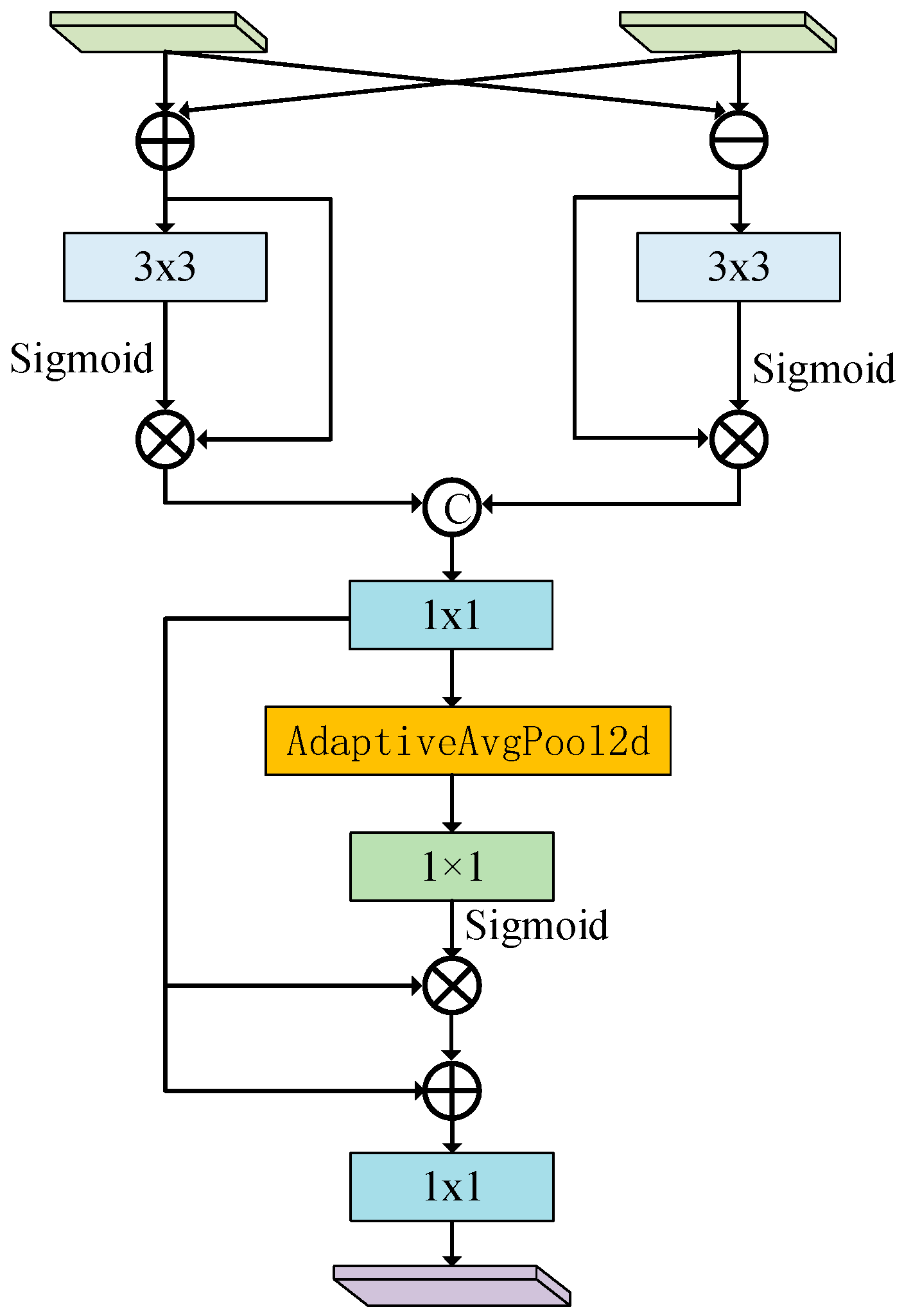
2.4. Feature-Difference Enhancement Module (FDEM)

In the field of remote-sensing image-change detection based on deep learning, selecting a suitable similarity measurement method plays a key role in extracting highly discriminative features from the network. Highly discriminative features can not only significantly improve the robustness of the model, so that it can still maintain stable performance under complex and changeable environments but can also effectively reduce the interference of pseudo-changes on detection results, thereby improving the accuracy and reliability of the detection. In a related study, Daudt et al. [30] proposed two methods for obtaining change information, namely, the difference method and the concatenation method, which operate based on the bi-temporal feature graph. By calculating the difference between the bi-temporal feature maps, the difference method can show the changed region more clearly, making the change information more prominent on the feature maps. However, this approach has certain limitations. When the bi-temporal image is faced with the problem of inconsistent imaging angles or large registration errors, the difference method may introduce more error information, resulting in the deviation of detection results. In contrast, the concatenation method fully retains the feature information of bi-temporal images by concatenating feature maps, thereby comprehensively covering various image details. However, it is less effective in explicitly identifying changed regions compared to the difference method, making the change information less conspicuous in the overall features.

To further amplify change-relevant features, the FDEM integrates both subtraction and concatenation operations to distinguish changed and unchanged regions. This design addresses the limitations of traditional similarity measures. As shown in Figure 4, the FDEM synergistically combines these two methods while avoiding their respective disadvantages. The module aims to organically integrate the difference method and the concatenation method, and through reasonable design and operation, the module can highlight the changed region more accurately on the basis of retaining the complete feature information and in order to strengthen the model’s ability to capture and process the change information and provide strong support for more accurate remote-sensing image-change detection.

In the process of difference feature extraction, the FDEM focuses on highlighting the difference information between the two input feature maps. Specifically, an element-by-element difference operation is performed on the two input feature graphs first. Assume that the input feature maps are $f_1$ and $f_2$, whose shapes are both $R^{B\times C\times H\times W}$, where $B$ represents the batch size, $C$ is the channel count and $H$ and $W$ are the height and width of the feature maps, respectively. The difference calculation result $f_D$, too, has the shape $R^{B\times C\times H\times W}$. Then, the difference feature map $f_D$ is sent into the processing flow composed of convolutional layer and Sigmoid function, and then the processed difference feature map is multiplied with the initial difference feature map element-by-element to achieve the weighted difference feature, enhancing the feature expression of the changed region and gaining the final difference feature map $f_D^{\prime }$. This map can clearly highlight the change between the two input feature maps and provide key clues for the subsequent accurate detection of the changed region. In contrast to difference feature extraction, similar feature extraction aims to capture the common information between two input feature maps. First, the two input feature graphs are summed element-by-element to obtain $f_S$, which is also $R^{B\times C\times H\times W}$ in shape. Then, similar to the difference feature extraction, convolution and Sigmoid transformation are performed on the summative feature maps $f_S$, and the same weighting operation is performed on the similar feature maps to obtain the similar feature maps $f_S^{\prime }$. Similar feature maps $f_S^{\prime }$ can effectively retain the feature information of relatively stable and unchanged regions in the two input feature maps. After the extraction of the difference feature map $f_D^{\prime }$ and the similar feature map $f_S^{\prime }$, the FDEM concatenates them along the channel dimension. Since they have the same spatial dimensions $H$ and $W$, the concatenation operation can be carried out smoothly, and the concatenated feature map $f_C$ can be obtained, at which time the number of channels becomes $2C$. Then, the convolution layer is adopted for further feature fusion of the concatenated feature map. This process can deeply integrate the difference information and similar information, so that the feature map not only contains the significant features of the changed region, but also retains the stable features of the unchanged region, thus significantly improving the expression ability of the features. To further optimize the quality of the fused feature maps, the global-average pooling operation is carried out on the fused feature maps. Global-averaging pooling averages the feature maps of each channel in spatial dimensions to obtain a vector of length $C$, which is used to compress spatial information into statistical information of the channel dimension, thus focusing on the importance differences between channels. Then, the attention map $f_C^{\prime }$ is obtained by convolution operation and Sigmoid function transformation on the pooled results. The shape of the attention map $f_C^{\prime }$ is consistent with the fused feature map in channel dimension, and its value represents the importance of each channel feature. Finally, the attention map $f_C^{\prime }$ and the fused feature map are weighted to get the final result map $f_{out}$. In this way, the network can focus more on the feature information that is important for change detection, and further enhance the feature expression ability. The above mathematical expression is as follows:

$$f_D=f_1-f_2,$$

(9)

$$f_D^{\prime }=f_D\otimes \sigma \left(f_{•}^{3\times 3}\left(f_D\right)\right),$$

(10)

$$f_S=f_1+f_2,$$

(11)

$$f_S^{\prime }=f_S\otimes \sigma \left(f_{•}^{3\times 3}\left(f_S\right)\right),$$

(12)

$$f_C=\left[f_D^{\prime },f_S^{\prime }\right],$$

(13)

$$f_C^{\prime }=GAP\left(f^{1\times 1}\left(f_C\right)\right),$$

(14)

$$f_{out}=f^{1\times 1}\left(f_C+f_C\otimes \sigma \left(f_{•}^{1\times 1}\left(f_C^{\prime }\right)\right)\right),$$

(15)

where $f_{•}^{3\times 3}\left(\cdot \right)$ denotes the two-dimensional 3 × 3 convolution, with batch normalization; $GAP\left(\cdot \right)$ represents the global-average pooling layer; $f_{•}^{1\times 1}\left(\cdot \right)$ denotes the two-dimensional 1 × 1 convolution, with batch normalization and $f^{1\times 1}\left(\cdot \right)$ denotes the two-dimensional 1 × 1 convolution, with an ReLU activation function.

2.5. Dataset Materials

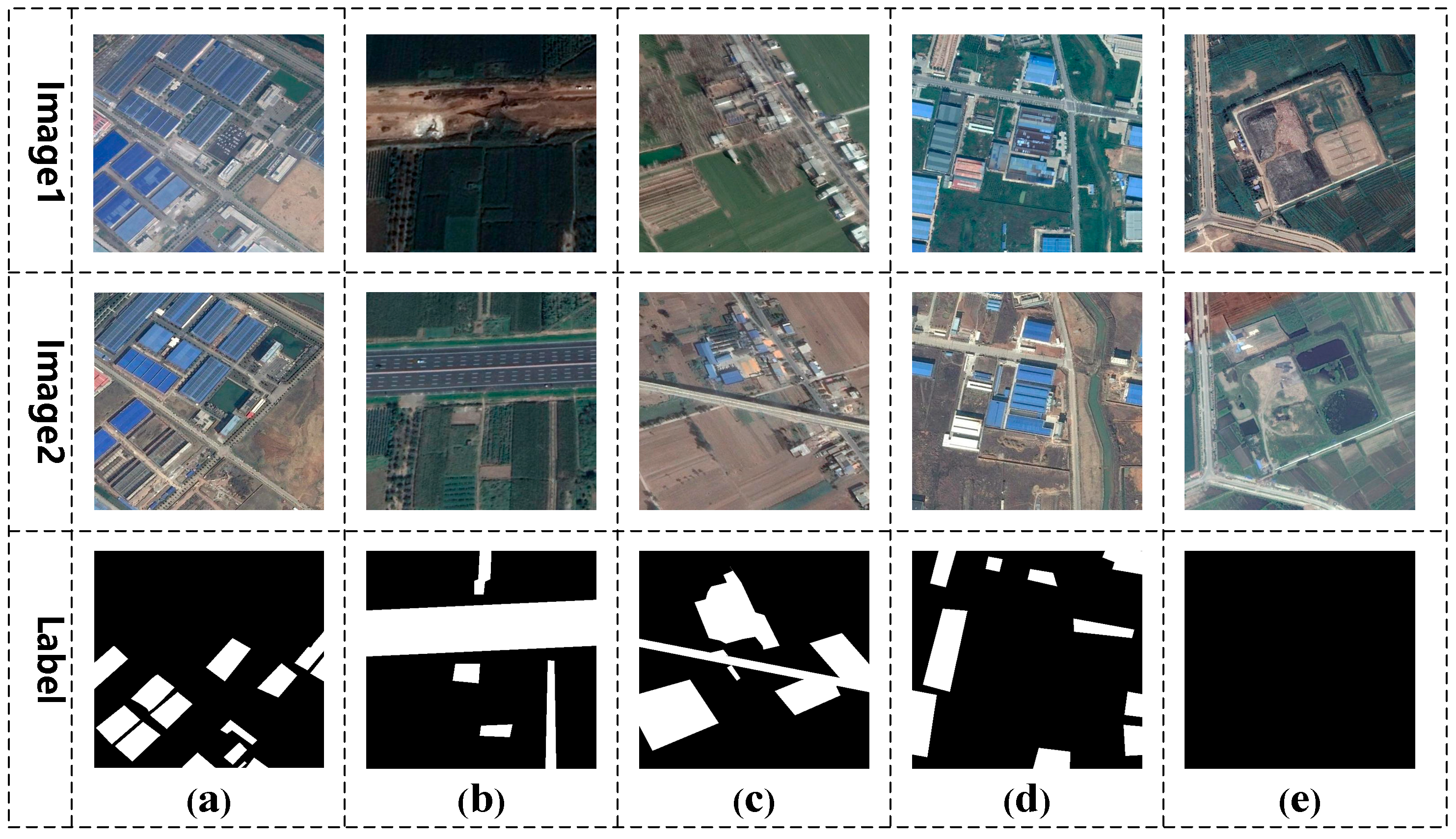
2.5.1. BTCDD Dataset

The BTCDD dataset, comprising 3420 pairs of bi-temporal remote-sensing images, was collected from Google Earth for model validation. These images capture diverse scenes in eastern China (2010–2019). The dataset was labeled, and uniform cropping was finished. Figure 5 shows representative samples with rich objects and change types. To mimic real-world scenarios, we included high-angle pairings, seasonal images and unchanged region pairs to better evaluate model performance.

To increase data sample diversity and quantity, data augmentation is needed for training image data expansion. Frequently employed methods include rotation, flipping, scaling, etc. They help deeply analyze image features, enhance the adaptability to different scenes and improve its generalization performance. When performing data augmentation, careful consideration of parameter configurations is critical for achieving optimal performance.

Table 2. Parameters for data augmentation.

Methods	Parameters
random rotation	−10 to 10°
translation	−20 to 20°
HSV saturation	−50 to 50%
random horizontal flip	50%
random vertical flip	50%

specifies stochastic geometric augmentation parameters: 50 percent probability for axial rotations (empirically constrained to ±10° to prevent excessive negative sample generation) and equivalent 50% saturation adjustment amplitude in HSV space. Spatial displacement operations were bounded at 20% of the image dimensions. Notably, these augmentation methods (expanding training samples to 13.68 k) were exclusively deployed during neural parameter optimization phases, while validation/testing phases strictly prohibited such transformations to maintain evaluation integrity.

Finally, these data augmentation methods obviously expand image samples in the training, as shown in Figure 6. This optimizes the generalization ability of the model, thus enhancing cross-scenario transferability under distribution shift conditions.

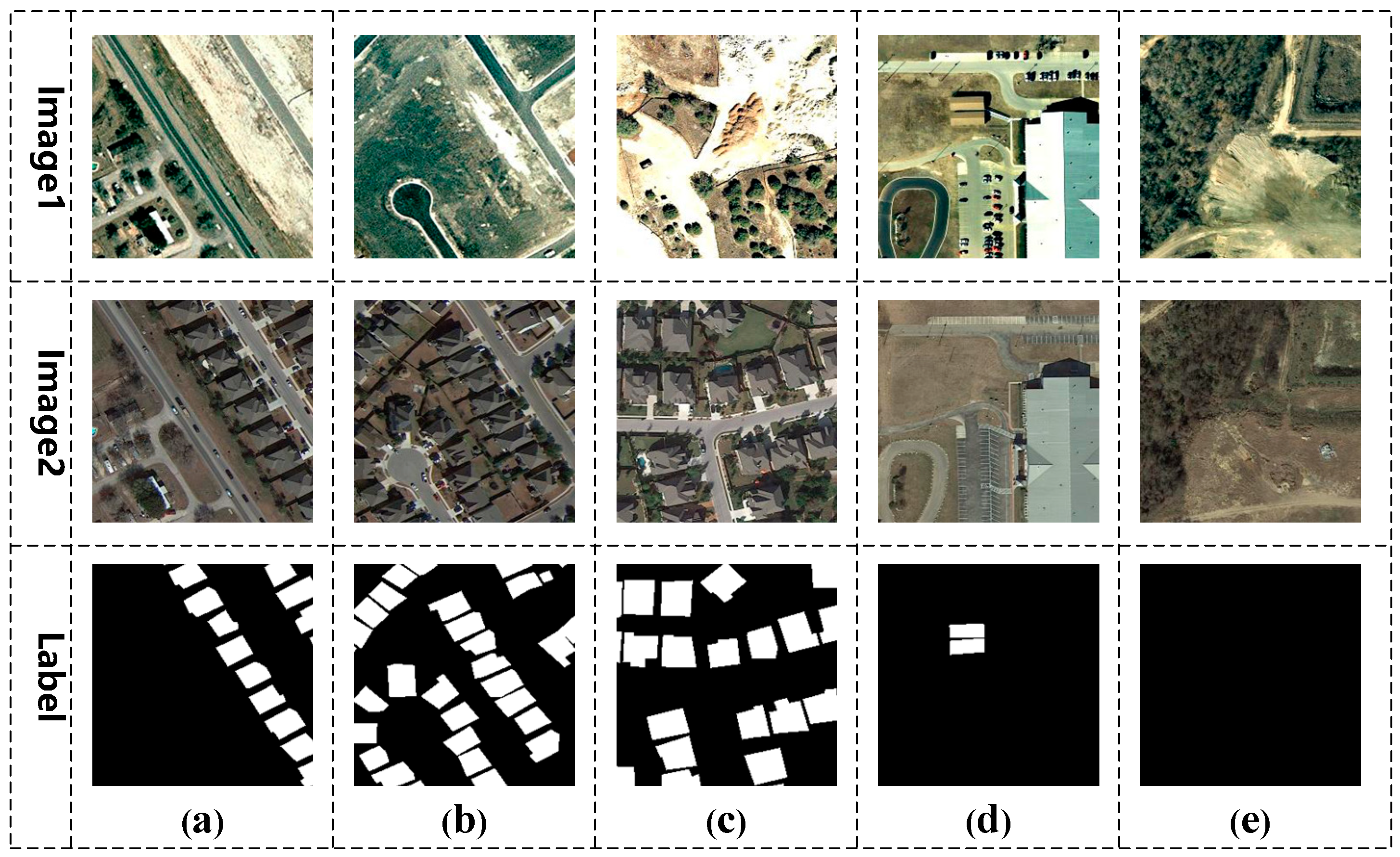
2.5.2. LEVIR-CD Dataset

LEVIR-CD is a large dataset used to detect changes in buildings [31], with high resolution (1024 × 1024 pixels) Google Earth images. It focuses on images with significant land use changes. As shown in Figure 7, we selected three types of building images: new buildings, disappearing buildings and unchanged buildings. Each sample was cropped into 16 256 × 256 small blocks, generating 7120 image block pairs for training, 1024 for validation and 2048 for testing.

2.5.3. BCDD Dataset

The BCDD dataset was published by Ji et al. [32], as shown in Figure 8. After splitting, a total of 1858 image pairs were cropped, and then, 1116 images were selected for data expansion. The operation was the same as that of the BTCDD dataset method, and 6696 image pairs were obtained as the training set, as shown in Figure 9. A total of 371 pairs were used as verification sets and 371 pairs as test sets.

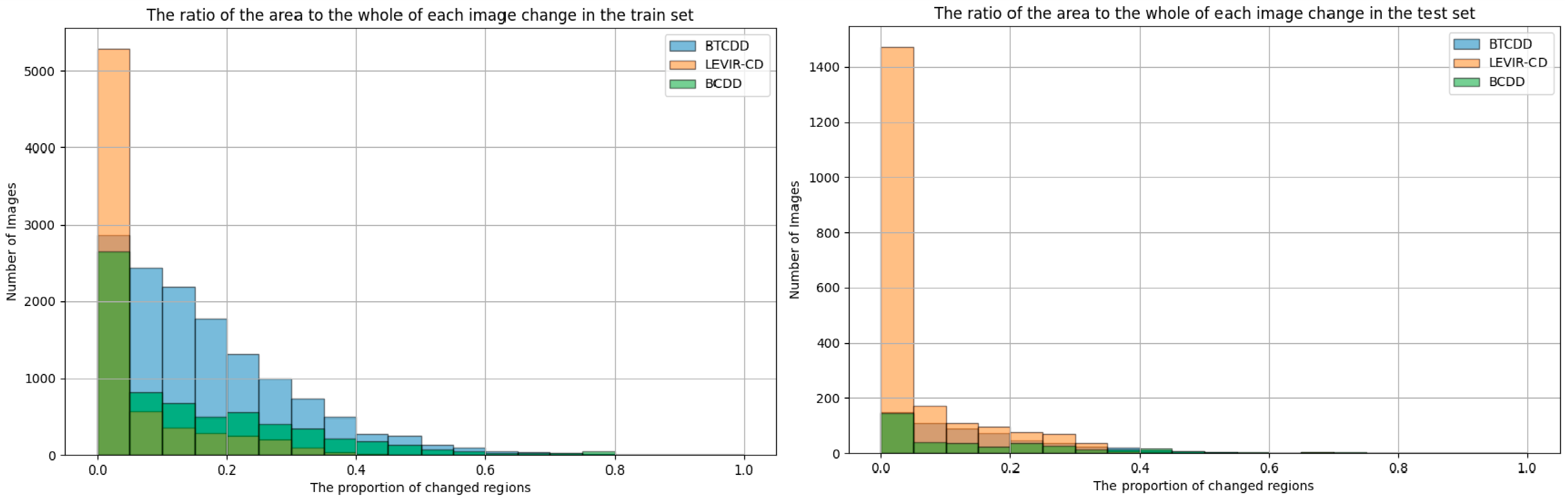
2.5.4. Data Analysis

To verify the validity, we tested on a laboratory’s own dataset and two open-access datasets. First, through analyzing changed parts of every image, we will acquire a more thorough comprehension of elements of the dataset.

Table 3. Statistics of changed and unchanged pixels in the BTCDD, LEVIR-CD and BCDD datasets.

Dataset		Changed Pixels	Unchanged Pixels	Proportion
BTCDD	train	589,780,588	2,996,349,332	0.196
	val	31,424,441	117,997,639	0.266
	test	21,277,278	128,144,802	0.166
	total	642,482,307	3,242,491,773	0.198
LEVIR-CD	train	21,412,971	445,203,349	0.048
	val	3,668,682	63,440,147	0.058
	test	6,837,404	127,380,324	0.054
	total	31,919,057	636,023,820	0.050
BCDD	train	65,215,450	373,613,606	0.174
	val	4,132,500	20,181,356	0.205
	test	3,751,149	20,562,707	0.182
	total	73,099,099	414,357,669	0.176

shows that three datasets contain a small proportion of changed regions compared with the unchanged regions.

For greater visual clarity, we count images with distinct proportion levels. As shown in Figure 10, the horizontal coordinate is the proportion of the changed regions in the whole, and the vertical coordinate is the number of images in this proportion. From the data analysis chart, the proportion of changed area in most of the data is less than 20%.

2.6. Performance Evaluation Metrics

To systematically assess the effectiveness of diverse change-detection algorithms comprehensively and impartially, a set of objective quantitative metrics system is introduced in this study. The specific approach is to carefully compare the prediction results of each algorithm with the real label graph, so as to achieve the accurate quantitative evaluation of the algorithm performance. Since the core task of change detection is classification, this experiment selects the key metrics in the field of classification to evaluate the effect of change detection. This includes overall accuracy (OA), recall rate (RC), precision (PR), F1 score and Mean Intersection over Union (Miou). OA represents the predicted correct proportion of all pixels, RC represents the proportion of the changes accurately identified by the algorithm in the real changes of the original image and PR measures the proportion of pixels correctly identified as changed regions in the forecast map in the total number of pixels in the real reference change area. The F1 score is adopted to assess the overall prediction outcome, and the higher the value, the better the prediction quality. By calculating the intersection and union ratio of two sets, the Miou clearly presents the changed and unchanged regions in the change-detection task. Through the comprehensive use of the above multiple-evaluation metrics, the model effectiveness can be assessed more comprehensively and thoroughly. The relevant formulas are as follows:

$$OA={\displaystyle \frac{TP+TN}{TP+TN+FP+FN}},$$

(16)

$$Recall={\displaystyle \frac{TP}{TP+FN}},$$

(17)

$$Precision={\displaystyle \frac{TP}{TP+FP}},$$

(18)

$$F1={\displaystyle \frac{2\times PR\times RC}{PR+RC}},$$

(19)

$$Miou={\displaystyle \frac{TP}{TP+FP+FN}},$$

(20)

In the formulas, $TP$ denotes true positive, the correctly identified changed region; $FP$ denotes false positive, in which unchanged regions are erroneously predicted as changed regions; $TN$ denotes true negative, the unchanged regions of correct prediction and $FN$ denotes false negative, signifying the incorrect prediction of a changed region as an unchanged region.

The above evaluation metrics are widely used in classification tasks. Based on these five-evaluation metrics, this paper carries out performance evaluation of the proposed change detection model to fully verify its advancement and effectiveness. In addition, to measure the efficiency of diverse change-detection networks, two metrics (parameters (Params) and floating-point operations (FLOPs)) are also introduced in this paper to comprehensively evaluate the change-detection algorithm in this paper.

3. Experimental

3.1. Experimental Environment

The experiments in this paper are based on pytorch and RTX3070Ti. We use Adam gradient descent as our network optimizer and BCEWithLogitsLoss as our network loss function. The selection of learning rate in deep-learning tasks is very important; if the learning rate is too high, the loss value will explode and the model will not converge, and if the learning rate is too low, the complexity of the fusion network will be greatly increased and the model will be difficult to converge. In this study, ABLRCNet, a lightweight model to be developed, was developed on three datasets: BTCDD, LEVIR-CD and BCDD, with seven different change detection models (FC_EF, FC-Siam-Diff, FC-Siam-Conc [30], SNUNet [33], ChangeNet [34], TCDNet [35], DASNet [36] and six common deep-learning models (FCN8s [37], SegNet [38], UNet [39], HRNet [40], DeepLabV3+ [41] and BiseNet [42]) were compared from multiple key dimensions, and all models used the same parameters on the dataset, with the initial learning rate set to 0.001, the decay index set to 0.9, the batch size set to eight and the maximum number of training iterations set to 200. We evaluate the performance of each model holistically and from multiple perspectives based on multiple dimensions such as model complexity (FLOPs), number of parameters (Params) and F1 and MIoU scores, which are critical for change-detection tasks.

3.2. Network Module Ablation Experiment

As deep understanding and verification of the developed modules will successfully improve accuracy of the model, we add and remove modules on the three datasets BTCDD, LEVIR-CD and BCDD.

Table 4. Ablation experiments of ABLRCNet. (bold numbers represent the optimal results).

	Method	LRCB	LRCB + SAM	LRCB + MSAM	LRCB + MSAM + FDEM
Dataset
BTCDD	OA (%)	94.84	94.87	95.1	95.55
	RC (%)	70.48	72.24	74.28	73.87
	PR (%)	77.15	75.25	76.36	77.79
	F1 (%)	71.76	72.3	73.66	74.14
	MIoU (%)	80.21	80.94	81.52	82.24
LEVIR-CD	OA (%)	97.69	97.98	98.08	98.19
	RC (%)	77.32	78.17	78.21	78.46
	PR (%)	79.56	81.74	82.18	83.25
	F1 (%)	77.64	79.32	79.87	80.19
	MIoU (%)	82.96	84.24	84.85	85.41
BCDD	OA (%)	96.57	96.73	96.98	97.12
	RC (%)	75.28	75.62	75.97	76.68
	PR (%)	74.24	74.68	75.12	75.3
	F1 (%)	72.83	73.21	73.52	74.01
	MIoU (%)	80.14	81.2	81.32	82.74

displays the results of the ablation experiment. As a basic model, the LRCB obtains a series of basic performance data on the BTCDD, LEVIR-CD and BCDD datasets. In the BTCDD dataset, OA was 94.84%, RC was 70.48%, PR was 77.15%, F1 was 71.76% and the MIoU was 80.21%. In the LEVIR-CD dataset, OA was 97.69%, RC was 77.32%, PR was 79.56%, F1 was 77.64% and the MIoU was 82.96%. In the BCDD dataset, OA was 96.57%, RC was 75.28%, PR was 74.24%, F1 was 72.83% and the MIoU was 80.14%. Subsequently, different auxiliary modules were added on the basis of the LRCB for the experiments. After the addition of a SAM, a number of metrics on each dataset were improved, such as in the BTCDD dataset, the F1 score was increased from 71.76% to 72.30% and the MIoU was increased from 80.21% to 80.94%, indicating that the module can optimize the model performance. Compared with the LRCB + SAM combination, the addition of an MSAM has a more significant performance improvement. On the BTCDD dataset, the F1 score was significantly increased to 73.66%, and the MIoU was increased to 81.52%, indicating its stronger ability to process multi-scale feature information. The addition of the FDEM also further optimizes performance, with the MIoU increasing to 82.24% on the BTCDD dataset.

Through the analysis of the ablation experiment results of each dataset, it can be seen that compared with the SAM, the LRCB adding the MSAM can obtain better performance improvement, which proves the high efficiency of the MSAM. At the same time, the FDEM and other auxiliary modules have significantly improved and optimized the overall network performance. When multiple modules work collaboratively on the backbone network, all metrics on the three datasets show a positive improvement trend, reducing prediction errors and omissions, accurately detecting the change region and providing a strong basis and direction for the optimization of remote-sensing image-change detection models.

As shown in

Table 5. Comparison of ablation experimental processing time (on the BTCDD dataset).

Method	Processing Time (ms/Image)	Parameters (M)	FLOPs (G)
LRCB	0.041	7.12	9.88
LRCB + SAM	0.042	7.13	9.91
LRCB + MSAM	0.048	9.04	12.91
LRCB + MSAM + FDEM	0.051	13.57	16.13

, the processing time increases progressively with the addition of the attention and enhancement modules. LRCB + MSAM + FDEM introduces a 24.4% increase in inference time compared to the baseline LRCB (51 ms vs. 41 ms) due to the computational overhead of the multi-scale convolutions in the MSAM and feature fusion in the FDEM. However, this trade-off yields significant accuracy improvements: the MIoU increases by 2.03% on BTCDD, 2.45% on LEVIR-CD and 2.6% on BCDD dataset, demonstrating that the modules effectively balance efficiency and performance for real-time applications with moderate computational budgets.

Figure 11 shows the comparison of the SAM and MSAM heat maps on the BTCDD, LEVIR-CD and BCDD datasets, where (a) and (b) are the original image; (c) is the label; (d) is the heat map of the network without adding the attention module; (e) is the heat map with the SAM added and (f) is heat maps with the MSAM added. For regions with insufficient initial attention or area focusing errors, the feature map uses the red to represent the regions with high attention and uses the blue and green to represent the regions with low weight. Subsequent to the adoption of the MSAM, feature maps evidently show improved efficiency and accuracy in focusing on these areas.

3.3. Ablation Experiment of the Feature-Difference Enhancement Module

In this section, we make different arrangements and combinations of the difference method, concatenation method and connection method in the feature difference enhancement module on the three datasets of BTCDD, LEVIR-CD and BCDD.

The + represents the addition of feature maps, the − represents the subtraction of feature maps, and c represents the concatenation of feature maps. (+−, c) means that the two input feature maps are added and subtracted by parallel double branches first, and then concatenated; (+c, −) indicates that the two input feature maps are added and concatenated in parallel, and then subtracted; (−c, +) indicates that the two input feature maps are subtracted and concatenated in parallel, and then added.

Table 6. Ablation experiments of the feature-difference enhancement module (bold numbers represent the optimal results).

	Method	ABLRCNet (+−, c)	ABLRCNet (+c, −)	ABLRCNet (−c, +)
Dataset
BTCDD	OA(%)	95.55	95.21	94.82
	RC(%)	73.87	74.27	73.64
	PR(%)	77.79	77.56	76.91
	F1(%)	74.14	73.82	73.65
	MIoU(%)	82.24	82.02	81.91
LEVIR-CD	OA(%)	98.19	98.08	98.02
	RC(%)	78.46	78.84	78.36
	PR(%)	83.25	82.94	82.87
	F1(%)	80.19	80.06	79.97
	MIoU(%)	85.41	85.29	84.96
BCDD	OA(%)	97.12	96.94	96.53
	RC(%)	76.68	76.53	76.31
	PR(%)	75.3	74.84	74.62
	F1(%)	74.01	73.71	73.62
	MIoU(%)	82.74	82.42	82.13

displays the experimental results of the different combinations.

As can be seen from Table 6, F1 and the MIoU of ABLRCNet (+−, c) in the BTCDD dataset are 74.14% and 82.24%, and F1 and the MIoU of the LEVIR-CD dataset are 80.19% and 85.41%, respectively. In BCDD dataset, F1 was 74.01 % and the MIoU was 82.74%. The combination first performs the addition and subtraction operations of the feature graphs in parallel, so that the similarity and difference information between feature graphs can be mined simultaneously. It is then concatenated to fuse different types of information together. In subsequent operations, such as adaptive average pooling, the rich and diverse feature information offers a broader basis for model learning, so that the model can better extract and use these features. ABLRCNet (+c, −) had 73.82% F1 and 82.02% MIoU in the BTCDD dataset, 80.06% F1 and 85.29% MIoU in the LEVIR-CD dataset and 73.71% F1 and 82.42% MIoU in the BCDD dataset. The combination firstly adds and concatenates the feature maps in parallel, which strengthens the similarity of the feature maps and realizes the information fusion initially. However, the subsequent subtraction operation may mistakenly delete some beneficial differential features of the model in the process of removing part of the information, resulting in damage to the integrity of the features and further affecting the performance of the model, so it is slightly lower than the combination of ABLRCNet (+−, c) in some metrics of the three datasets. ABLRCNet (−c, +) had 73.65% F1 and 82.02% MIoU in the BTCDD dataset, 79.97% F1 and 84.96% MIoU in the LEVIR-CD dataset and 73.62% F1 and 82.13% MIoU in the BCDD dataset. The combination first subtracts and concatenates, then overfocuses on differences between the feature maps, resulting in the loss of some similarity information. However, in the subsequent addition operation, due to the incomplete feature information in the early stage, the feature complementarity is insufficient, and it is difficult for the model to obtain enough key information in the learning process, which ultimately makes the metrics of the combination on the three datasets relatively lower.

3.4. Comparative Experiments on BTCDD Dataset

In order to avoid duplication, we only analyzed the parameter quantities (Params), complexity (FLOPs) and the MIoU and F1 scores of the models on the BTCDD dataset to evaluate the performance of each model in a comprehensive and multi-angle manner, and in order to present these complex comparative data in a more intuitive and clear way, we drew a scatter plot (as shown in Figure 12).

It can be clearly observed from the figure that ABLRCNet achieves significant reduction in the two key metrics of model complexity and parameter counts compared with other comparison models. This achievement not only reflects the excellent advantages of ABLRCNet in model weight, but also means that it is expected to complete efficient change-detection tasks with lower computing resource consumption and storage requirements in practical applications. It is particularly worth mentioning that in F1 score and MIoU value, two core metrics to measure the accuracy and performance of model detection, ABLRCNet has made significant improvements compared with traditional change-detection models and common deep-learning models.

Table 7. Comparison of quantitative results of different algorithms on the BTCDD dataset (bold numbers represent the optimal results).

Method	OA (%)	RC (%)	PR (%)	F1 (%)	MioU (%)	FLOPs (G)	Params (M)	Time (ms)
FC_EF	90.32	40.4	69.3	45.67	64.83	5.52	1.35	14.372
FC-Siam-Diff	91.55	46.56	73.30	52.46	68.36	9.29	1.35	16.258
FC-Siam-Conc	91.51	53.79	69.21	56.62	69.97	9.34	1.55	12.994
FCN8s	92.93	64.44	67.41	63.91	74.41	80.68	18.65	9.09
SNUNet	92.98	64.02	69.24	64.22	74.41	175.76	12.03	0.017
SegNet	93.75	64.38	72.75	66.62	76.28	160.72	29.45	10.526
ChangeNet	94.02	61.08	75.24	65.35	76.29	42.73	23.52	28.897
UNet	93.89	65.11	73.53	67.15	76.86	124.21	13.4	9.893
HRNet	94.10	66.80	74.21	68.18	77.61	85.62	4.49	33.243
TCDNet	94.38	68.24	77.22	70.11	79.03	27.56	22.91	20.005
DeepLabV3+	94.39	67.63	74.62	68.92	78.17	89.15	59.35	32.932
BiseNet	94.81	67.86	77.6	70.59	79.71	24.87	31.26	14.696
DASNet	95.08	69.12	79.42	72.35	81.23	115.79	50.27	23.142
ABLRCNet	95.55	73.87	77.79	74.14	82.24	16.13	13.57	0.051

shows the results of various evaluation metrics of different algorithms on the BTCDD dataset. All deep-learning models use uniform training parameters to ensure fairness. The FC_EF model shows the weakest performance, with an F1 score of only 45.67% and a MIoU score of 64.83%. The lightweight ABLRCNet network proposed in this paper has achieved significant breakthroughs through architecture innovation, showing multiple advantages in core metrics. In terms of performance, the OA of ABLRCNet is 95.55%, far exceeding that of FC_EF (90.32%). Compared to some models that perform better in the field of segmentation, such as SegNet, UNet and DASNet, ABLRCNet still shows a good effect. In terms of RC and PR metrics, ABLRCNet is significantly better than FC_EF (40.4% and 69.3%) by 73.87% and 77.79%, respectively, and the key metric, F1 score, increases to 74.14%, an increase of more than 60% compared with FC_EF. The F1 score of FC-Siam-Diff is 52.46%, and the F1 score of FC-Siam-Conc is 56.62%, which are much lower than ABLRCNet. The MloU metric reaches 82.24%, which is 17.41% higher than that of FC_EF. More notably, the FLOPs metric is only 16.13 G and Params is 13.57 M, which is significantly lower than FCN8s (80.68 G/18.65 M) and SNUNet (175.76 G/12.03 M). Compared with FC_EF (5.52 G/1.35 M), although the number of parameters increases slightly, the overall performance achieves a qualitative leap. The results show that ABLRCNet can effectively solve the pain points of a deep-learning model with large number of parameters and high computing cost and provide a better solution for real-time image processing tasks while maintaining the performance of mainstream models.

Figure 13 presents prediction results of different models on the bi-temporal image, visually showing the performance of different algorithms in the change-detection task. Through careful comparison of visualization results, it can be seen that although the remaining 13 deep-learning and change-detection algorithms can roughly determine the changed region, they all have the problem of false detection or missing detection to varying degrees. For example, in some images, some algorithms mistakenly mark the unchanged region as the changed region, resulting in false detection. In other cases, the subtle changes that actually exist are not accurately identified, and the phenomenon of missing detection occurs. Among them, FC_EF, FC-Siam-Diff, FC-Siam-Conc and other algorithms only adopt simple feature extraction in the coding stage and rely on upsampling fusion in the decoding stage, which makes it difficult to accurately capture complex changes in images. These algorithms are prone to bias when dealing with regions with fine structure or small changes and cannot fully and accurately reflect the real changes. In contrast, our proposed Siamese ABLRCNet significantly improves the accuracy and precision of change detection through the innovative addition of the MSAM and FDEM to the LRCB, especially the full use of the MSAM at the encoder and decoder stages. The MSAM can focus on the changed region and the unchanged region, and through in-depth analysis and differentiation of the features of the different regions, the model can effectively enhance the understanding of complex scenes. This allows ABLRCNet to not only identify regions of change more accurately, but also to perform well in the optimization of edge details, with predictions that closely resemble real labels.

3.5. Generalization Experiments on the LEVIR-CD and BCDD Datasets

In order to verify the adaptability of ABLRCNet on the datasets, we performed a generalization experiment, selected the public LEVIR-CD and BCDD datasets, and discussed the model complexity, parameter counts, F1 score and MIoU value with other change-detection algorithms in recent years.

Table 8. Experiments with different algorithms on the LEVIR-CD and BCDD datasets. (Numbers in bold indicate the results of our model).

	Dataset	LEVIR-CD (%)					BCDD (%)					Performance Evaluation
Method		OA	RC	PR	F1	MIoU	OA	RC	PR	F1	MIoU	FLOPs (G)	Params (M)
FC_EF		97.73	77.08	77.43	75.75	82.54	95.77	65.83	70.04	65.13	77.14	1.19	1.35
FC-Siam-Diff		97.99	78.15	80.74	78.60	84.24	94.06	71.99	63.97	64.61	75.41	2.32	1.35
FC-Siam-Conc		97.96	81.09	80.73	79.59	84.56	91.93	76.55	58.06	62.05	72.31	2.33	1.55
FCN8s		98.11	79.29	82.18	79.71	84.96	96.89	74.22	66.74	65.78	77.82	20.17	18.65
SNUNet		98.16	82.44	82.21	81.13	85.58	96.01	77.38	69.86	70.45	79.47	43.94	12.03
SegNet		97.91	78.18	79.93	77.52	83.53	96.58	76.42	77.83	74.45	81.63	40.18	29.45
ChangeNet		97.59	79.57	76.30	76.51	82.47	95.39	73.52	66.77	67.02	77.56	10.68	23.52
UNet		98.31	80.27	83.20	80.53	85.84	96.43	71.43	73.67	74.56	82.42	31.05	13.4
HRNet		98.13	78.37	82.17	79.14	84.78	96.62	73.34	75.45	71.53	81.32	21.4	4.49
TCDNet		97.66	77.24	79.36	77.26	82.93	96.97	74.83	75.47	73.12	81.79	6.89	22.91
BiseNet		97.75	77.75	79.97	77.91	83.38	97.26	75.14	74.61	73.17	82.11	6.22	31.26
DeepLabV3+		98.07	80.08	82.13	80.12	85.06	97.31	74.41	75.68	73.31	82.16	22.29	59.35
DASNet		97.88	80.24	80.85	78.56	84.72	96.15	72.23	74.36	71.24	80.72	28.95	50.27
ABLRCNet		98.19	78.46	83.25	80.19	85.41	97.12	76.68	75.3	74.01	82.74	4.03	13.57

presents the results of various evaluation metrics of diverse algorithms on the LEVIR-CD and BCDD datasets. First, let’s look at the situation of the LEVIR-CD dataset. F1 score is one key metric to evaluate the capability of the model, considering the accuracy and recall rate of the model. SNUNet achieved the highest F1 score of 81.13% among all comparison models, indicating a good balance between accuracy and completeness of the detection results. UNett followed with 80.53%, also performing very well. ABLRCNet’s F1 score of 80.19% is also at a high level, ranking high among many models. From the perspective of overall data distribution, F1 scores of most of the tested models are concentrated between 75% and 80%, and ABLRCNet can achieve a high score than this interval, which proves its effectiveness in change-detection tasks. The MIoU reflects the degree of overlap between the model prediction results and the real label, and the higher the value, the higher the prediction accuracy of the model. UNet achieved 85.84% on the MIoU metric showing a high alignment between its forecast results and the real situation. SNUNet ranked second with 85.58%, also showing excellent detection accuracy. The MIoU of ABLRCNet is 85.41%, which is very small gap with the top two, indicating its excellent performance in detection accuracy. In general, there are certain differences among models in the MIoU metric, and the outstanding performance of ABLRCNet in this key performance metric further verifies its high-precision advantage in change-detection tasks.

Then, let’s look at the situation on the BCDD dataset. The ABLRCNet model exhibits specific performance characteristics. OA is 97.12%, which is in the second tier of comparison algorithms, slightly lower than DeepLabV3+’s 97.31%, but higher than SNUNet (96.01%) and UNet (96.43%). F1 scored 74.01%, slightly lower than UNet’s 74.56%, but better than ChangeNet (67.02%) and FC-EF (65.13%), suggesting that there is still potential for enhancement in the balance of accuracy (75.30%) and recall (76.68%). The MIoU is 82.74%; it is the highest among all algorithms, indicating that its segmentation accuracy for the change region is at the cutting-edge level.

The metric FLOPs is adopted to evaluate the computational complexity of the model. The lower FLOPs metric, the lower the computational cost of the model. Among the comparison models, FC_EF has the lowest FLOPs score at 1.19 G, giving it a significant advantage in terms of computing resource requirements. The FLOPs score of ABLRCNet is 4.03 G, which is also at a low level, far lower than UNet’s (31.05 G), SegNet’s (40.18 G) and SNUNet’s (43.94 G). A low FLOPs score means that ABLRCNet can complete change-detection tasks with less computing resource consumption in practical applications, especially in scenarios with limited computing resources. The number of parameters is another important measure of the model’s complexity, and a smaller parameter number generally means that the model has lower storage requirements and may also reduce the risk of overfitting. The parameter number of ABLRCNet is 13.57 M, which is lower than that of many models, such as BiseNet (31.26 M), DeepLabV3+ (59.35 M) and DASNet (50.27 M). This shows that ABLRCNet can effectively control the number of parameters, reduce the storage cost and training difficulty of the model and make it more advantageous in actual deployment through reasonable architecture design, ensuring the model’s capacity.

Figure 14 shows the prediction results of various models on the LEVIR-CD image, which intuitively shows the capacity of different algorithms in the change-detection task. Through careful comparison of the visualization results, it can be seen that although the remaining 13 deep-learning and change-detection algorithms can roughly determine the change region, they all have the issue of false detection or missing detection to varying degrees (red indicates missing detection, blue indicates false detection). For example, FC_EF is not capable of handling small area changes or complex changes, and TCDNet is not fine enough to handle the edges of changes. In change detection, contextual information is very important to accurately determine the changed region. These models do not make full use of the contextual information of the image, resulting in an inaccurate definition of the boundary of the changing region. FC-Siam-Diff, FC-Siam-Conc and other algorithms detect the changed region to a certain extent, but they are not sufficient to extract some complex or subtle features. For example, FC-Siam-Diff missed more targets with small changes, indicating that its feature extraction module could not effectively identify the features of these small targets. In the actual remote-sensing image, there are various interference factors, such as noise, different lighting conditions and so on. These models may be weak in anti-interference, resulting in the accuracy and stability of detection results. SNUNet models adopt an effective feature fusion strategy, which can integrate features of different levels and types, so as to identify the changed region more accurately. However, they still have the problem of missing detection when dealing with small objects. These algorithms are prone to bias when dealing with regions with fine structure or small changes and cannot fully and accurately reflect the real changes. In contrast, our proposed lightweight network ABLRCNet, with Siamese architecture, significantly improves the accuracy and precision of change detection by adding the MSAM and FDEM to the LRCB, especially in the full use of the MSAM at the encoder and decoder stages. The MSAM can focus on changed regions and unchanged regions, and through in-depth analysis and differentiation of features of different regions, the model can effectively enhance the understanding of complex scenes. This allows ABLRCNet to not only identify changed regions more accurately, but also to perform well in the optimization of edge details, with predictions that closely resemble real labels.

Figure 15 displays prediction results of diverse models on the BCDD graphs, and clearly shows the performance of the different algorithms in change-detection tasks. Through careful comparison of the visualization results, it can be seen that most algorithms have the following common problems: (1) rough edge segmentation, such as FC-Siam-Conc, FC-Siam-Diff and other algorithms. In groups (I) and (II) images, the edge of the changed region of the prediction graph is significantly offset from the label. It reflects that the ability to extract and integrate spatial features is insufficient, and the changing boundary cannot be accurately described. (2) Insufficient processing of large-area changes: in the large-area change scenario of group (III), although some algorithms can detect the main changed area, they have the problem of rough edges or incomplete internal filling, and the integration ability of global features of large-area scenes is insufficient, resulting in deviations between the detection results and the real labels. (3) Poor adaptability to complex scenes: In group (II), affected by the complexity of ground objects, the false detection area in the prediction map exceeds the range of the real labels, indicating that the suppression ability of background interference is insufficient. In group (I) of TCDNet, the edge segmentation of the changed region is fuzzy, and the precision is insufficient. ABLRCNet’s prediction maps show a significantly high degree of alignment with the labels: Enhanced feature analysis through modules such as the MSAM can accurately focus on the real changed region. For example, in group (III) change detection, the changed region can be completely marked, and the edge details are fine. In groups (I) and (II), the phenomena of false detection and missing detection are significantly less than that of other algorithms, reflecting its innovative advantages in feature fusion and context understanding and effectively improving the accuracy and precision in complex scenes.

4. Discussion

This paper focuses on the attention-based lightweight remote-sensing change-detection network (ABLRCNet) to carry out in-depth research and discussion. In the context of the swift advancement of remote-sensing technology, the conventional detection methods face many difficulties; ABLRCNet aims to address the challenge of balancing computational efficiency and detection accuracy. In terms of network design, ABLRCNet innovatively incorporates lightweight residual convolutional blocks (LRCBs), multi-scale spatial-attention modules (MSAMs) and feature-difference enhancement modules (FDEMs). LRCBs can extract features effectively while reducing calculation cost through ingenious structure design. Inspired by the spatial-attention mechanism, the MSAM integrates spatial information of diverse scales to enhance the model’s capacity to perceive local details and global semantics. The FDEM’s flexibly combines the difference method and concatenation method, which significantly improves the ability to capture and process change information. The experiment is comprehensive and in-depth, covering a variety of experiment types. In the visualization of the attention heat map, the advantages of the MSAM in focusing key areas are intuitively demonstrated. Ablation experiments show that the MSAM, FDEM and other auxiliary modules significantly strengthen the capacity of the model, and the effect is better when multiple modules cooperate. The selection experiment of the feature-difference enhancement module confirms the influence of different arrangement and combination methods on the model performance and provides a basis for module optimization. In comparison and generalization experiments on the BTCDD, LEVIR-CD and BCDD datasets, ABLRCNet achieved significant improvement in detection accuracy while ensuring lightweightedness, showing strong competitiveness compared with a variety of traditional and deep-learning models. Although ABLRCNet is slightly inferior to some individual models in some metrics, it has remarkable results in the optimization of model complexity and parameter counts, especially for scenarios with limited computing resources. The follow-up research can further explore the optimization direction to strengthen the capacity of the model in complex scenarios, promote the remote-sensing change-detection technology to a new height and provide more efficient and accurate technical support for many fields, such as urban expansion monitoring and ecological environment assessment.

References

1. Liu, Y.; Wu, L.Z. Geological Disaster Recognition on Optical Remote Sensing Images Using Deep Learning. Procedia Comput. Sci. 2016, 91, 566–575. [Google Scholar] [CrossRef]
2. Chughtai, A.H.; Abbasi, H.; Karas, I.R. A review on change detection method and accuracy assessment for land use land cover. Remote Sens. Appl. Soc. Environ. 2021, 22, 100482. [Google Scholar] [CrossRef]
3. Cheng, P.; Xia, M.; Wang, D.; Lin, H.; Zhao, Z. Transformer Self-Attention Change Detection Network with Frozen Parameters. Appl. Sci. 2025, 15, 3349. [Google Scholar] [CrossRef]
4. Tison, C.; Nicolas, J.-M.; Tupin, F.; Maitre, H. A new statistical model for Markovian classification of urban areas in high-resolution SAR images. IEEE Trans. Geosci. Remote. Sens. 2004, 42, 2046–2057. [Google Scholar] [CrossRef]
5. Papadomanolaki, M.; Vakalopoulou, M.; Karantzalos, K. A deep multitask learning framework coupling semantic segmentation and fully convolutional LSTM networks for urban change detection. IEEE Trans. Geosci. Remote. Sens. 2021, 59, 7651–7668. [Google Scholar] [CrossRef]
6. Zhu, T.; Zhao, Z.; Xia, M.; Huang, J.; Weng, L.; Hu, K.; Lin, H.; Zhao, W. FTA-Net: Frequency-Temporal-Aware Network for Remote Sensing Change Detection. IEEE J. Sel. Top. Appl. Earth Obs. Remote. Sens. 2025, 18, 3448–3460. [Google Scholar] [CrossRef]
7. Isaienkov, K.; Yushchuk, M.; Khramtsov, V.; Seliverstov, O. Deep learning for regular change detection in Ukrainian forest ecosystem with sentinel-2. IEEE J. Sel. Top. Appl. Earth Obs. Remote Sens. 2020, 14, 364–376. [Google Scholar] [CrossRef]
8. Zhan, Z.; Ren, H.; Xia, M.; Lin, H.; Wang, X.; Li, X. AMFNet: Attention-guided multi-scale fusion network for bi-temporal change detection in remote sensing images. Remote. Sens. 2024, 16, 1765. [Google Scholar] [CrossRef]
9. Sublime, J.; Kalinicheva, E. Automatic post-disaster damage mapping using deep-learning techniques for change detection: Case study of the Tohoku tsunami. Remote. Sens. 2019, 11, 1123. [Google Scholar] [CrossRef]
10. Ke, L.; Lin, Y.; Zeng, Z.; Zhang, L.; Meng, L. Adaptive Change Detection With Significance Test. IEEE Access 2018, 6, 27442–27450. [Google Scholar] [CrossRef]
11. Rignot, E.J.M.; Van Zyl, J.J. Change detection techniques for ERS-1 SAR data. IEEE Trans. Geosci. Remote Sens. 1993, 31, 896–906. [Google Scholar] [CrossRef]
12. Zhuang, H.; Deng, K.; Fan, H.; Yu, M. Strategies Combining Spectral Angle Mapper and Change Vector Analysis to Unsupervised Change Detection in Multispectral Images. IEEE Geosci. Remote Sens. Lett. 2016, 13, 681–685. [Google Scholar] [CrossRef]
13. Li, Y.; Weng, L.; Xia, M.; Hu, K.; Lin, H. Multi-scale fusion siamese network based on three-branch attention mechanism for high-resolution remote sensing image change detection. Remote Sens. 2024, 16, 1665. [Google Scholar] [CrossRef]
14. Lefebvre, A.; Corpetti, T.; Hubertmoy, L. Object-Oriented Approach and Texture Analysis for Change Detection in Very High Resolution Images. In Proceedings of the IEEE International Geoscience & Remote Sensing Symposium, Boston, MA, USA, 7–11 July 2008; pp. 1005–1013. [Google Scholar]
15. Juan, S.U. A Change Detection Algorithm for Man-made Objects Based on Multi-temporal Remote Sensing Images. Acta Autom. Sin. 2008, 34, 13–19. [Google Scholar]
16. Benedek, C.; Sziranyi, T. Change Detection in Optical Aerial Images by a Multilayer Conditional Mixed Markov Model. IEEE Trans. Geosci. Remote Sens. 2009, 47, 3416–3430. [Google Scholar] [CrossRef]
17. Wang, W.; Liu, C.; Liu, G.; Wang, X. CF-GCN: Graph convolutional network for change detection in remote sensing images. IEEE Trans. Geosci. Remote Sens. 2024, 62, 5607013. [Google Scholar] [CrossRef]
18. Chen, J.; Yuan, Z.; Peng, J.; Chen, L.; Huang, H.; Zhu, J.; Liu, Y.; Li, H. DASNet: Dual attentive fully convolutional Siamese networks for change detection in high-resolution satellite images. IEEE J. Sel. Top. Appl. Earth Obs. Remote Sens. 2020, 14, 1194–1206. [Google Scholar] [CrossRef]
19. Ding, A.; Zhang, Q.; Zhou, X.; Dai, B. Automatic recognition of landslide based on CNN and texture change detection. In Proceedings of the 2016 31st Youth Academic Annual Conference of Chinese Association of Automation (YAC), Wuhan, China, 11–13 November 2016; IEEE: Piscataway, NJ, USA, 2016; pp. 444–448. [Google Scholar]
20. Hou, B.; Wang, Y.; Liu, Q. Change detection based on deep features and low rank. IEEE Geosci. Remote Sens. Lett. 2017, 14, 2418–2422. [Google Scholar] [CrossRef]
21. Zhan, Y.; Fu, K.; Yan, M.; Sun, X.; Wang, H.; Qiu, X. Change detection based on deep siamese convolutional network for optical aerial images. IEEE Geosci. Remote Sens. Lett. 2017, 14, 1845–1849. [Google Scholar] [CrossRef]
22. Zhang, X.; Li, W.; Gao, C.; Yang, Y.; Chang, K. Hyperspectral pathology image classification using dimension-driven multi-path attention residual network. Expert Syst. Appl. 2023, 230, 120615. [Google Scholar] [CrossRef]
23. Wang, F.; Wu, Y.; Zhang, Q.; Zhang, P.; Li, M.; Lu, Y. Unsupervised Change Detection on SAR Images Using Triplet Markov Field Model. IEEE Geosci. Remote Sens. Lett. 2013, 10, 697–701. [Google Scholar] [CrossRef]
24. Zhang, W.; Lu, X. The spectral-spatial joint learning for change detection in multispectral imagery. Remote Sens. 2019, 11, 240. [Google Scholar] [CrossRef]
25. Ye, X.; Zhang, W.; Li, Y.; Luo, W. Mobilenetv3-yolov4-sonar: Object detection model based on lightweight network for forward-looking sonar image. In Proceedings of the OCEANS 2021: San Diego–Porto, Virtual, 20–23 September 2021; IEEE: Piscataway, NJ, USA, 2021; pp. 1–6. [Google Scholar]
26. Chen, Z.; Ji, H.; Zhang, Y.; Liu, W.; Zhu, Z. Hybrid receptive field network for small object detection on drone view. Chin. J. Aeronaut. 2025, 38, 103127. [Google Scholar] [CrossRef]
27. Lei, T.; Wang, J.; Ning, H.; Wang, X.; Xue, D.; Wang, Q.; Nandi, A.K. Difference enhancement and spatial–spectral nonlocal network for change detection in VHR remote sensing images. IEEE Trans. Geosci. Remote Sens. 2021, 60, 4507013. [Google Scholar] [CrossRef]
28. Ding, X.; Guo, Y.; Ding, G.; Han, J. Acnet: Strengthening the kernel skeletons for powerful cnn via asymmetric convolution blocks. In Proceedings of the IEEE/CVF International Conference on Computer Vision, Seoul, Republic of Korea, 27 October–2 November 2019; pp. 1911–1920. [Google Scholar]
29. Jiang, S.; Lin, H.; Ren, H.; Hu, Z.; Weng, L.; Xia, M. Mdanet: A high-resolution city change detection network based on difference and attention mechanisms under multi-scale feature fusion. Remote Sens. 2024, 16, 1387. [Google Scholar] [CrossRef]
30. Daudt, R.C.; Le Saux, B.; Boulch, A. Fully convolutional siamese networks for change detection. In Proceedings of the 2018 25th IEEE International Conference on Image Processing (ICIP), Athens, Greece, 7–10 October 2018; IEEE: Piscataway, NJ, USA, 2018; pp. 4063–4067. [Google Scholar]
31. Chen, H.; Shi, Z. A spatial-temporal attention-based method and a new dataset for remote sensing image change detection. Remote Sens. 2020, 12, 1662. [Google Scholar] [CrossRef]
32. Ji, S.; Wei, S.; Lu, M. Fully convolutional networks for multisource building extraction from an open aerial and satellite imagery data set. IEEE Trans. Geosci. Remote Sens. 2018, 57, 574–586. [Google Scholar] [CrossRef]
33. Miao, L.; Li, X.; Zhou, X.; Yao, L.; Deng, Y.; Hang, T.; Zhou, Y.; Yang, H. SNUNet3+: A full-scale connected Siamese network and a dataset for cultivated land change detection in high-resolution remote-sensing images. IEEE Trans. Geosci. Remote Sens. 2023, 62, 4400818. [Google Scholar] [CrossRef]
34. Ji, D.; Gao, S.; Tao, M.; Lu, H.; Zhao, F. Changenet: Multi-temporal asymmetric change detection dataset. In Proceedings of the ICASSP 2024—2024 IEEE International Conference on Acoustics, Speech and Signal Processing (ICASSP), Seoul, Republic of Korea, 14–19 April 2024; IEEE: Piscataway, NJ, USA, 2024; pp. 2725–2729. [Google Scholar]
35. Qian, J.; Xia, M.; Zhang, Y.; Liu, J.; Xu, Y. Tcdnet: Trilateral change detection network for google earth image. Remote Sens. 2020, 12, 2669. [Google Scholar] [CrossRef]
36. Li, Z.; Tang, C.; Wang, L.; Zomaya, A.Y. Remote sensing change detection via temporal feature interaction and guided refinement. IEEE Trans. Geosci. Remote Sens. 2022, 60, 5628711. [Google Scholar] [CrossRef]
37. Wu, C.; Du, B.; Zhang, L. Fully convolutional change detection framework with generative adversarial network for unsupervised, weakly supervised and regional supervised change detection. IEEE Trans. Pattern Anal. Mach. Intell. 2023, 45, 9774–9788. [Google Scholar] [CrossRef] [PubMed]
38. Zhao, X.; Wu, Z.; Chen, Y.; Zhou, W.; Wei, M. Fine-Grained High-Resolution Remote Sensing Image Change Detection by SAM-UNet Change Detection Model. Remote Sens. 2024, 16, 3620. [Google Scholar] [CrossRef]
39. Medical Image Computing and Computer-Assisted Intervention–MICCAI 2015. In Proceedings of the 18th International Conference, Munich, Germany, 5–9 October 2015; Proceedings, Part III 18. Springer: Berlin/Heidelberg, Germany, 2015; pp. 234–241.
40. Jiang, H.; Peng, M.; Zhong, Y.; Xie, H.; Hao, Z.; Lin, J.; Ma, X.; Hu, X. A survey on deep learning-based change detection from high-resolution remote sensing images. Remote Sens. 2022, 14, 1552. [Google Scholar] [CrossRef]
41. Li, Y. The research on landslide detection in remote sensing images based on improved DeepLabv3+ method. Sci. Rep. 2025, 15, 7957. [Google Scholar] [CrossRef]
42. Wang, Z.; Gu, G.; Xia, M.; Weng, L.; Hu, K. Bitemporal attention sharing network for remote sensing image change detection. IEEE J. Sel. Top. Appl. Earth Obs. Remote Sens. 2024, 17, 10368–10379. [Google Scholar] [CrossRef]
Figure 1. Lightweight residual convolutional network (ABLRCNet) framework based on asymmetric convolution and attention coupling. It is mainly composed of an encoder–decoder and auxiliary modules, which are lightweight residual convolution blocks (LRCBs), multi-scale spatial-attention modules (MSAMs), and feature-difference enhancement module (FDEM).
Remotesensing 17 02226 g001
Figure 2. Lightweight residual convolution block (LRCB).
Remotesensing 17 02226 g002
Figure 3. Multi-scale spatial-attention module (MSAM).
Remotesensing 17 02226 g003
Figure 4. Feature-difference enhancement module (FDEM).
Remotesensing 17 02226 g004
Figure 5. The BTCDD dataset map shows the changing areas and invariant areas of factories, highways and farmland. (ae) Denote factory, farmland, a road, a building and an unchanged area, respectively.
Remotesensing 17 02226 g005
Figure 6. BTCDD diagram of different data augmentation methods. (a) Original image; (b) original image rotated by 10 degrees; (c) translated image; (d) image after HSV transformation; (e) horizontally flipped image and (f) vertically flipped image.
Remotesensing 17 02226 g006
Figure 7. LEVIR-CD dataset. (ac) shows the areas of added buildings, (d) shows the areas of removed buildings, and (e) shows the unchanged areas.
Remotesensing 17 02226 g007
Figure 8. BCDD dataset graph; the first line is the unchanged graph, the second line is the changed graph, and the third line is the labels. (ad) shows the changing areas, (e) shows the unchanged areas.
Remotesensing 17 02226 g008
Figure 9. Diverse data augmentation techniques on the BCDD dataset. (a) Initial image; (b) rotated 10°; (c) translated; (d) after HSV transformation; (e) horizontally flipped and (f) vertically flipped.
Remotesensing 17 02226 g009
Figure 10. The proportion of changed regions relative to the entire image in the dataset.
Remotesensing 17 02226 g010
Figure 11. Visualization of attention heat maps on the BTCDD, LEVIR-CD and BCDD datasets. (a,b) are the original images, (c) is labels, (d) is heatmaps of the network without the attention module added, (e) is the heatmaps of the SAM added and (f) is the heatmaps of the MSAM added.
Remotesensing 17 02226 g011
Figure 12. Performance comparison of different models on the BTCDD dataset.
Remotesensing 17 02226 g012
Figure 13. Comparison of prediction maps of several algorithms on the BTCDD dataset. (I), (II) and (III) indicate selected comparison images. Image1 and Image2 are bi-temporal remote-sensing images from different periods, and label is the set label. (an) indicate prediction maps of FC_EF, FC-Siam-Diff, FCN8s, FC-Siam-Conc, SNUNet, SegNet, ChangeNet, UNet, HRNet, DeepLabV3+, TCDNet, BiseNet, DASNet and ABLRCNet, respectively.
Remotesensing 17 02226 g013
Figure 14. Comparison of prediction maps of several algorithms on the LEVIR-CD dataset. (I), (II) and (III) indicate selected comparison images. Image1 and Image2 are bi-temporal remote sensing images from different periods, and label is the set label. (an) Indicate prediction maps of FC_EF, FC-Siam-Diff, FCN8s, FC-Siam-Conc, SNUNet, SegNet, ChangeNet, UNet, HRNet, DeepLabV3+, TCDNet, BiseNet, DASNet, and ABLRCNet, respectively.
Remotesensing 17 02226 g014
Figure 15. Comparison of prediction maps of several algorithms on the BCDD dataset. (I), (II) and (III) indicate selected comparison images. Image1 and Image2 are bi-temporal remote sensing images from different periods, and label represents the set label. (an) Indicate prediction maps of FC_EF, FC-Siam-Diff, FCN8s, FC-Siam-Conc, SNUNet, SegNet, ChangeNet, UNet, HRNet, DeepLabV3+, TCDNet, BiseNet, DASNet and ABLRCNet, respectively.
Remotesensing 17 02226 g015