

Multi-Scale Validation of Suspended Sediment Retrievals in Dynamic Estuaries: Integrating Geostationary and Low-Earth-Orbiting Optical Imagery for Hangzhou Bay
 ,
,
Abstract

1. Introduction
2. Materials and Methods
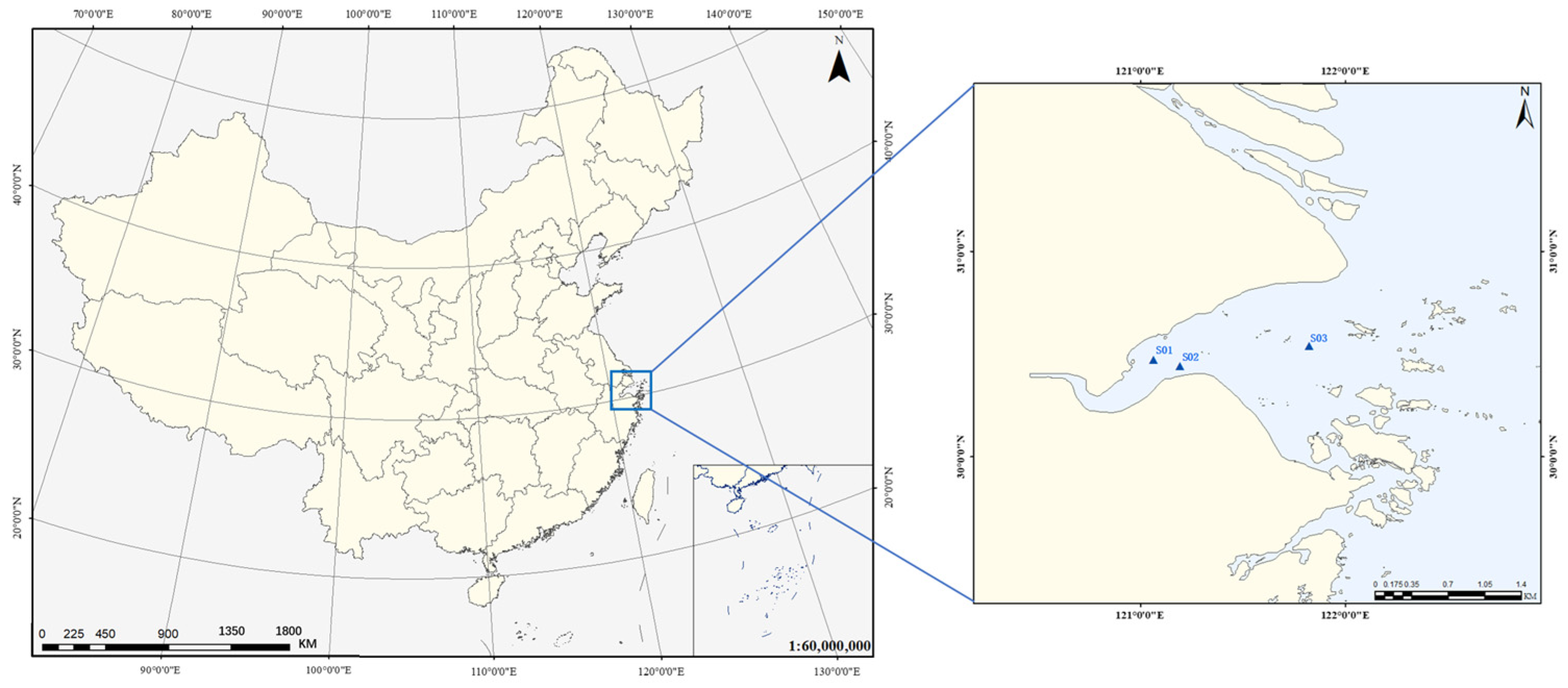
2.1. Study Area and In Situ Data
2.2. HJ-1A/B and GOCI Data
3. Comparative Retrieval of Suspended Sediment
3.1. Atmospheric Correction and Inversion Model Establishment
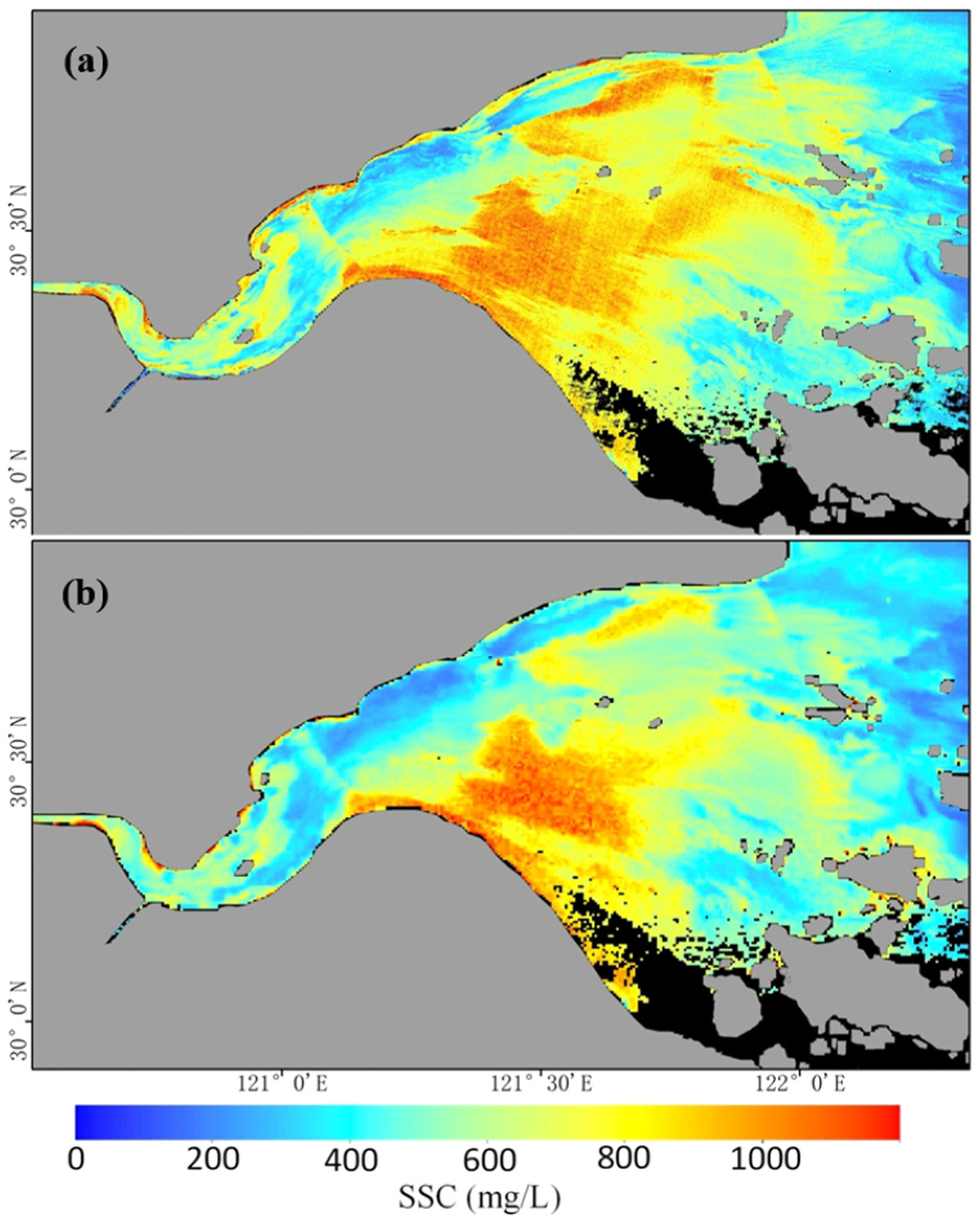
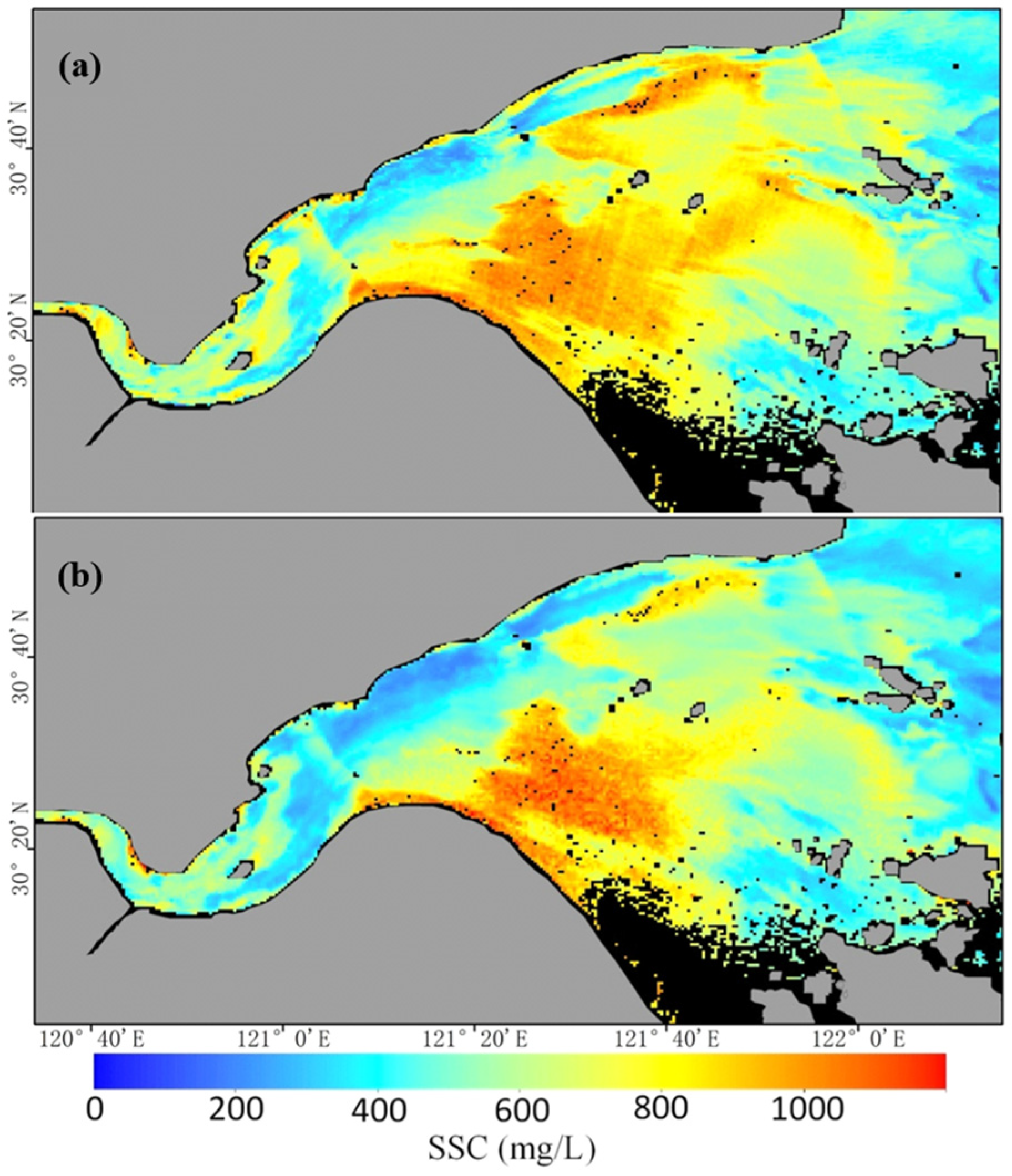
3.2. Comparative Sediment Retrieval Using Synchronous Imagery
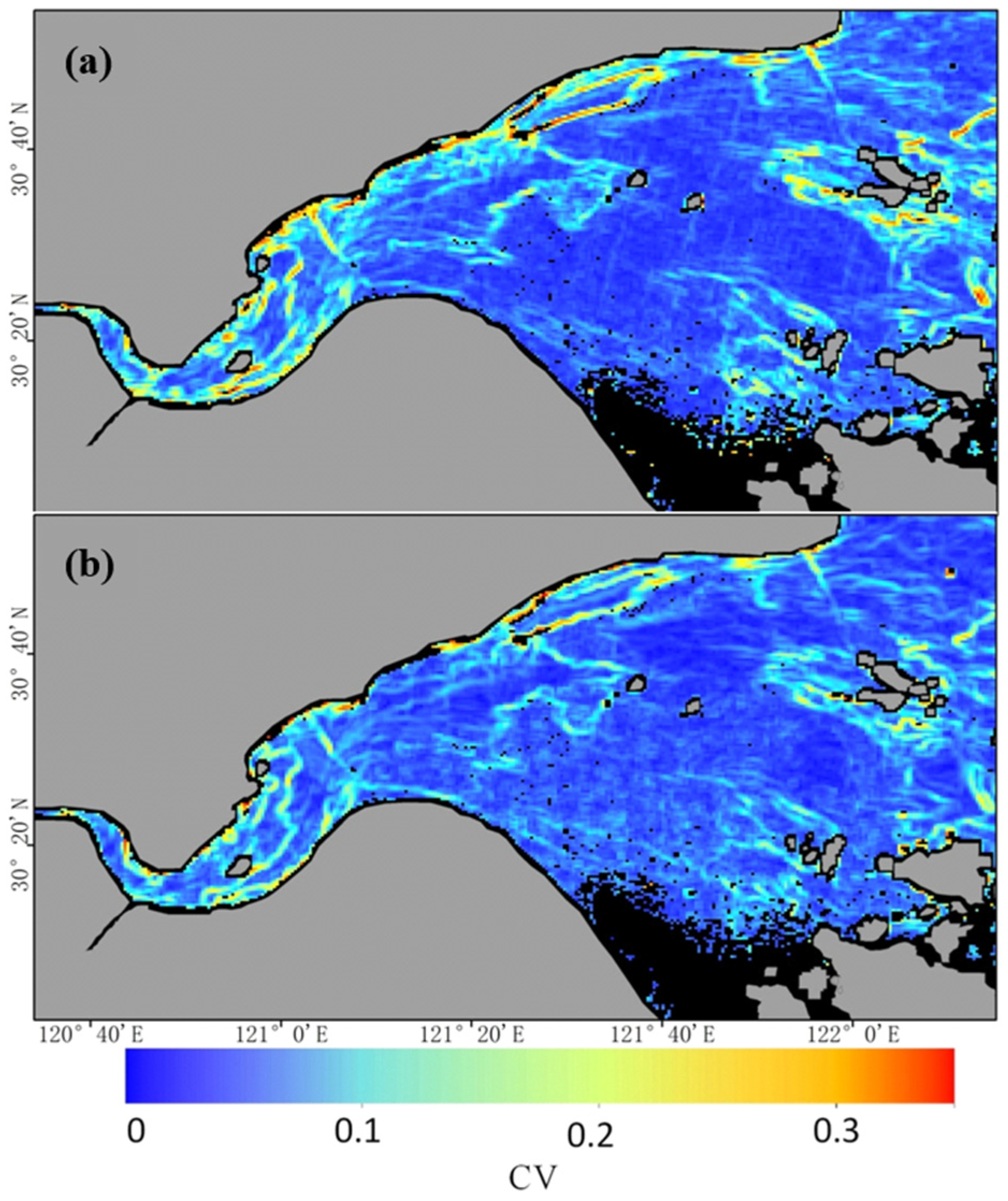
4. SSC Spatial Variability and CV Analysis
5. Evaluation of Scale Effects in the Validation of GOCI-Derived SSC
5.1. Limitations of Traditional Validation Methods
5.2. Proposed Method for Scale Effect Evaluation
- Apply appropriate atmospheric correction and SSC inversion models to retrieve the spatial distribution of SSC from both the GOCI image and the nearly simultaneous HJ CCD image and perform preliminary validation with a limited number of in situ data points.
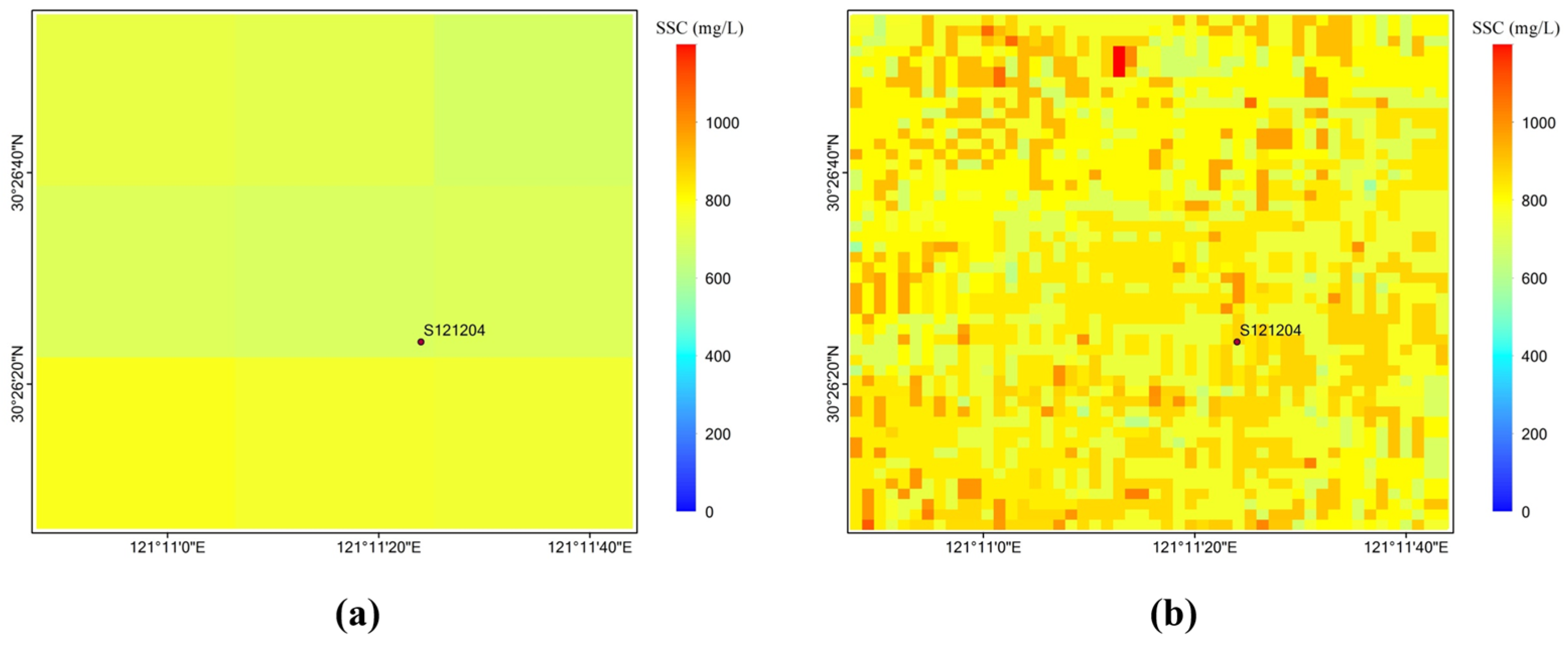
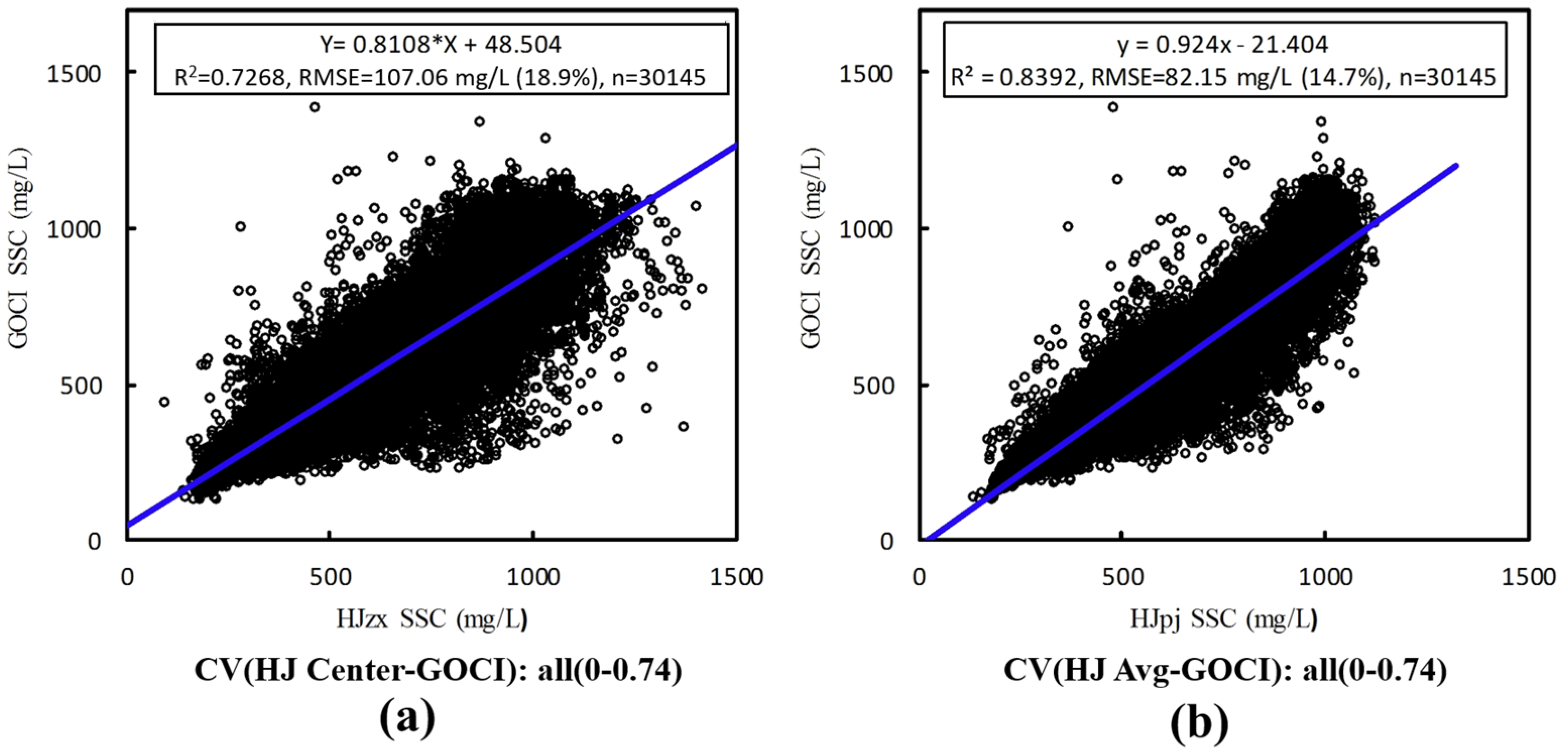
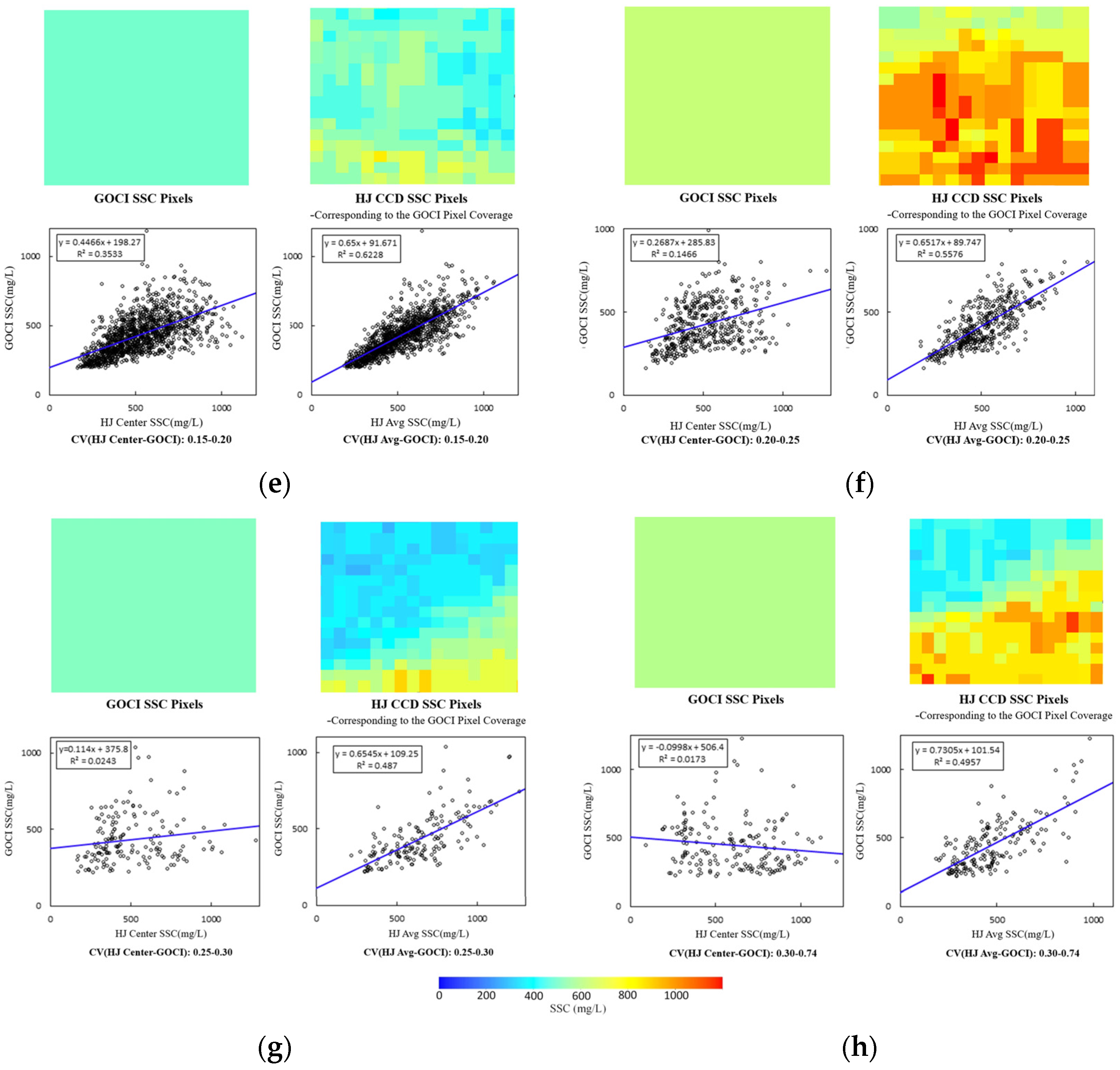
- Resample the 30 m HJ CCD SSC data to a 500 m resolution using two approaches: (a) compute the mean SSC over a 17 × 17 window corresponding to each 500 m GOCI pixel (denoted as HJ-Avg SSC); (b) use the central pixel’s SSC value from the corresponding 17 × 17 HJ CCD window (denoted as HJ-Center SSC).
- Calculate the CV of SSC for each 17 × 17 HJ CCD window corresponding to a GOCI pixel and stratify the CV values into different intervals.
- Within each CV interval, perform regression analyses between GOCI SSC and both HJ-Avg SSC and HJ-Center SSC, determining the RMSE, R2, and MRE for each relationship.
- Compare the regression results for the two resampling approaches to evaluate the influence of scale effects within different CV intervals.
6. Conclusions
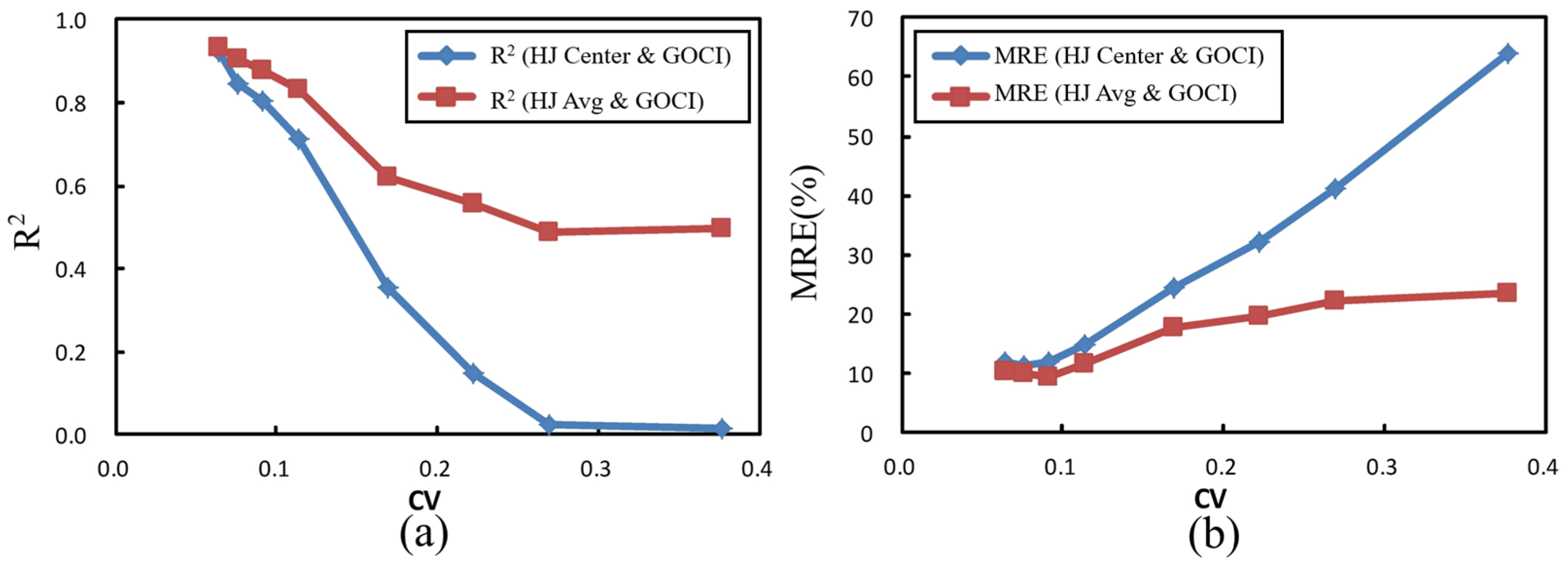
- Spatial averaging outperforms point-based validation: In regions with high spatial heterogeneity (CV > 0.10), the spatial averaging of HJ-CCD data (HJ-Avg) improved the correlation (R2) between HJ-CCD and GOCI retrievals by 17% and reduced the mean relative error (MRE) by 22% compared to central-pixel validation (HJ-Center). In zones where CV exceeds 0.15, HJ-Avg’s R2 decreases to approximately 0.80 and its MRE rises to around 13.5% (Table 6 and Figure 12). Nevertheless, this modest decline is much more gradual than the sharp degradation shown by HJ-Center, which falls to an R2 of 0.71 and an MRE of 14.89% under the same conditions. Such relative stability confirms the robustness of the spatial-averaging approach in highly dynamic areas.
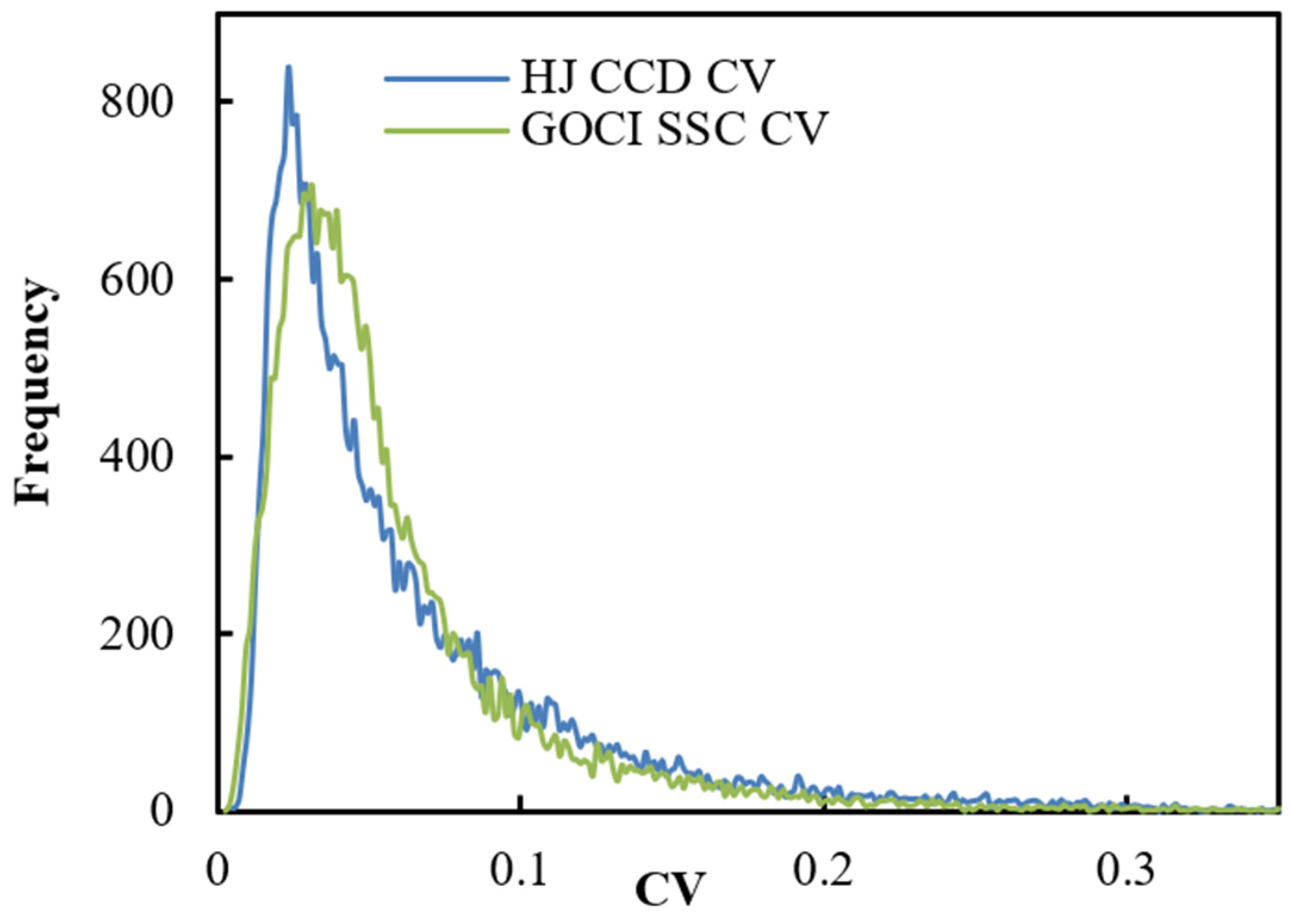
- The CV threshold defines scale effect dominance: A critical CV threshold of 0.10 was identified, beyond which scale effects dominate validation errors. This threshold aligns with Woodcock and Strahler’s scale theory [7], confirming that sensor resolution must match feature heterogeneity. Subpixel analysis revealed that HJ CCD resolved finer variability (CV up to 0.0944) compared to the GOCI (CV = 0.0528), directly addressing the first question posed in the Introduction on quantifying SSC spatial heterogeneity.
- Uncertainty reduction through multi-scale synergy: The framework reduced SSC validation uncertainty by 22%, lowering the RMSE from 107.06 mg/L (18.9% of the mean SSC) for traditional methods to 82.15 mg/L (14.7% of the mean) (Figure 10). This empirically answers the second question in the Introduction, demonstrating that spatial averaging—not single-point validation—is essential for mitigating scale effects in dynamic waters.
6.1. Innovation and Implications
- Operational standardization: The CV-based zoning framework provides the first quantitative criteria for scale-aware validation in coastal waters, adaptable to parameters like chlorophyll and CDOM.
- Methodological replicability: The workflow, leveraging nearly simultaneous data to isolate spatial scale effects, is transferable to other estuaries globally, such as the Mississippi Delta or Pearl River Estuary.
- Theoretical validation: The empirical confirmation of the 0.10 CV threshold reinforces the need for resolution–heterogeneity alignment in sensor design, echoing foundational remote sensing theories.
6.2. Limitations and Future Directions
Author Contributions
Funding
Data Availability Statement
Conflicts of Interest
References
- Hu, J.; Yu, Y.; Hu, W. Research on the technical framework for urban spatial database construction based on remote sensing imagery. Prog. Geogr. 2004, 23, 103–112. [Google Scholar]
- Tobler, W.R. A computer movie simulating urban growth in the Detroit region. Econ. Geogr. 1970, 46, 234–240. [Google Scholar] [CrossRef]
- Du, P.; Chen, Y.; Wang, X. Remote Sensing Science and Progress; China University of Mining and Technology Press: Xuzhou, China, 2007; pp. 154–196. [Google Scholar]
- Marceau, D.J.; Hay, G.J. Remote sensing contributions to the scale issue. Can. J. Remote Sens. 1999, 25, 357–366. [Google Scholar] [CrossRef]
- Li, J.; Tian, L.; Chen, X. Analysis of spatial scale error in quantitative remote sensing inversion of water environmental parameters. Acta Geodet. Cartogr. Sin. 2017, 46, 478–486. [Google Scholar]
- Hu, Y.; Yu, Z.; Zhou, B.; Li, Y.; Yin, S.; He, X.; Peng, X. Tidal-driven variation of suspended sediment in Hangzhou Bay based on GOCI data. Estuar. Coast. Shelf Sci. 2019, 217, 101920. [Google Scholar] [CrossRef]
- Woodcock, C.E.; Strahler, A.H. The factor of scale in remote sensing. Remote Sens. Environ. 1987, 21, 311–332. [Google Scholar] [CrossRef]
- Wu, H.; Li, Z.-L. Scale issues in remote sensing: A review on analysis, processing and modeling. Sensors 2009, 9, 1768–1793. [Google Scholar] [CrossRef]
- Bartkowiak, P.; Castelli, M.; Notarnicola, C. Downscaling land surface temperature from MODIS dataset with random forest approach over Alpine vegetated areas. Remote Sens. 2019, 11, 1319. [Google Scholar] [CrossRef]
- Kustas, W.P.; Norman, J.M.; Anderson, M.C.; French, A.N. Estimating subpixel surface temperatures and energy fluxes from the vegetation index-radiometric temperature relationship. Remote Sens. Environ. 2003, 85, 429–440. [Google Scholar] [CrossRef]
- Wang, Z.; Liu, C.; Huete, A. From AVHRR-NDVI to MODIS-EVI: Advances in vegetation index research. Acta Ecol. Sin. 2003, 23, 979–987. [Google Scholar]
- Guo, B.; Zhou, Y.; Wang, S.-X.; Tao, H.-P. The relationship between normalized difference vegetation index (NDVI) and climate factors in the semiarid region: A case study in Yalu Tsangpo River basin of Qinghai-Tibet Plateau. J. Mt. Sci. 2014, 11, 926–940. [Google Scholar] [CrossRef]
- Liu, L.; Cao, R.; Shen, M.; Chen, J.; Wang, J.; Zhang, X. How does scale effect influence spring vegetation phenology estimated from satellite-derived vegetation indexes? Remote Sens. 2019, 11, 2137. [Google Scholar] [CrossRef]
- Tayade, R.; Yoon, J.; Lay, L.; Khan, A.L.; Yoon, Y.; Kim, Y. Utilization of Spectral Indices for High-Throughput Phenotyping. Plants 2022, 11, 1712. [Google Scholar] [CrossRef] [PubMed]
- Peterson, K.T.; Martinez, M.J.; Gibson, C.J. Suspended sediment concentration estimation from Landsat imagery along the Lower Mississippi and Middle Mississippi Rivers using an extreme learning machine. Remote Sens. 2018, 10, 1503. [Google Scholar] [CrossRef]
- Pereira, F.J.S.; Costa, C.A.G.; Foerster, S.; Brosinsky, A.; de Araújo, J.C. Estimation of suspended sediment concentration in an intermittent river using multi-temporal high-resolution satellite imagery. Int. J. Appl. Earth Obs. Geoinf. 2019, 79, 153–161. [Google Scholar] [CrossRef]
- Kabir, S.M.I.; Ahmari, H. Evaluating the effect of sediment color on water radiance and suspended sediment concentration using digital imagery. J. Hydrol. 2020, 589, 125189. [Google Scholar] [CrossRef]
- Zhan, W.; Wu, J.; Wei, X.; Tang, S.; Zhan, H. Spatio-temporal variation of the suspended sediment concentration in the Pearl River Estuary observed by MODIS during 2003–2015. Cont. Shelf Res. 2019, 172, 22–33. [Google Scholar] [CrossRef]
- Pavelsky, T.M.; Smith, L.C. Remote sensing of suspended sediment concentration and hydrologic connectivity in a complex wetland environment. Remote Sens. Environ. 2013, 129, 197–209. [Google Scholar] [CrossRef]
- Liu, W.; Yu, Z.; Zhou, B.; Jiang, J.; Pan, Y.; Ling, Z. Assessment of suspended sediment concentration at Hangzhou Bay using HJ CCD imagery. J. Remote Sens. 2013, 17, 905–918. [Google Scholar] [CrossRef]
- Xu, Y.; Qin, B.; Zhu, G.; Zhang, Y.; Shi, K.; Li, Y.; Shi, Y.; Chen, L. High temporal resolution monitoring of suspended matter changes from GOCI measurements in Lake Taihu. Remote Sens. 2019, 11, 985. [Google Scholar] [CrossRef]
- Atkinson, P.M.; Tate, N.J. Spatial scale problems and geostatistical solutions: A review. Prof. Geogr. 2004, 52, 607–623. [Google Scholar] [CrossRef]
- Qiu, X.; Gao, H.; Wang, Y.; Zhang, W.; Shi, X.; Lv, F.; Yu, Y.; Luan, Z.; Wang, Q.; Zhao, X. A scale conversion model based on deep learning of UAV images. Remote Sens. 2023, 15, 2449. [Google Scholar] [CrossRef]
- Zhang, Y.; Sun, J.; Qiu, R.; Liu, H.; Zhang, X.; Xuan, J. Spatial scale effect of a typical polarized remote sensor on detecting ground objects. Sensors 2021, 21, 4418. [Google Scholar] [CrossRef]
- Gamon, J.A.; Wang, R.; Gholizadeh, H.; Ustin, S.L. Consideration of scale in remote sensing of biodiversity. In Remote Sensing of Plant Biodiversity; Springer International Publishing: Cham, Switzerland, 2020; pp. 425–447. [Google Scholar] [CrossRef]
- Froidefond, J.-M.; Gardel, L.; Guiral, D.; Parra, M.; Ternon, J.-F. Spectral remote sensing reflectances of coastal waters in French Guiana under the Amazon influence. Remote Sens. Environ. 2002, 80, 225–232. [Google Scholar] [CrossRef]
- Wu, H. Mechanism of suspended sediment transport and its response to tides in Hangzhou Bay. Acta Oceanol. Sin. 2006, 28, 1–10. [Google Scholar]
- Tang, J.W.; Tian, G.L.; Wang, X.Y.; Wang, X.M.; Song, Q.J. The Methods of Water Spectra Measurement and Analysis I: Above-Water Method. J. Remote Sens. 2004, 8, 37–44. [Google Scholar]
- Li, C.; Jia, Y.; Hu, J.; Li, Z. Analysis of the application prospects of HJ-1 optical satellite remote sensing. Remote Sens. Land. Resour. 2008, 3, 1–3. [Google Scholar]
- Cho, S.I.; Ahn, Y.H.; Ryu, J.H.; Kang, G.S.; Youn, H.S. Development of Geostationary Ocean Color Imager (GOCI). Korean J. Remote Sens. 2010, 26, 157–165. [Google Scholar]
- Yu, Z.; Chen, X.; Tian, L.; Zhou, W. Atmospheric Correction of HJ-1A/B CCD Imagery over Poyang Lake. Geomat. Inf. Sci. Wuhan Univ. 2012, 37, 1078–1082. [Google Scholar] [CrossRef]
- Tian, L.Q.; Lu, J.Z.; Chen, X.L.; Yu, Z.F.; Xiao, J.J.; Qiu, F.; Zhao, X. Atmospheric correction of HJ-1A/B CCD imageries over Chinese coastal waters using MODIS-Terra aerosol data. Sci. China Technol. Sci. 2010, 53, 191–195. [Google Scholar] [CrossRef]


| Imagery | Spatial Resolution (m) | Hangzhou Bay SSC (mg/L) | |||
|---|---|---|---|---|---|
| Minimum | Maximum | Mean | Standard Deviation | ||
| HJ CCD | 30 | 140.8 | 1533.4 | 627.0 | 215.3 |
| GOCI | 500 | 134.9 | 1512.9 | 566.4 | 206.7 |
| Sensor | Spatial Resolution (m) | CV | |||
|---|---|---|---|---|---|
| Minimum | Maximum | Mean | Standard Deviation | ||
| HJ CCD | 500 | 0.0043 | 0.3500 | 0.0638 | 0.0534 |
| GOCI | 500 | 0.0025 | 0.3499 | 0.0564 | 0.0441 |
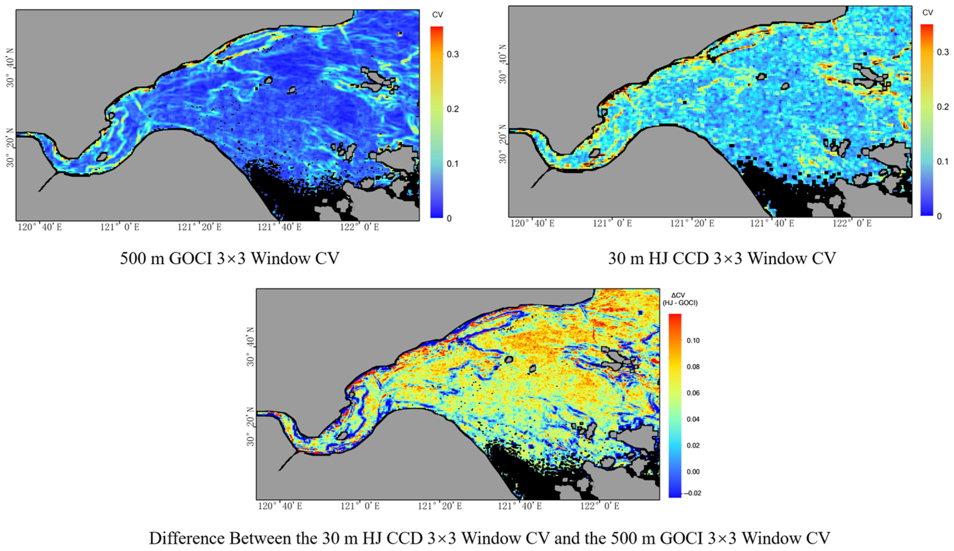
| CV | 3 3 Window Mean | Standard Deviation |
|---|---|---|
| 30 m HJ | 0.1078 | 0.0355 |
| 500 m GOCI | 0.0564 | 0.0441 |
| HJ-GOCI | 0.0514 | −0.0086 |
| Sensor | Spatial Resolution (m) | Imaging Time | SSC (mg/L) | ||
|---|---|---|---|---|---|
| Field Measurement | Image Inversion | R.E. (%) | |||
| HJ CCD | 30 | 10:39 | 993.20 | 827.9 | 16.65 |
| GOCI | 500 | 10:29 | 721.3 | 27.37 | |
| Sensor | Spatial Resolution (m) | Imaging Time | SSC (mg/L) | |||
|---|---|---|---|---|---|---|
| Field Measurement | Central Pixel | 3 3 Window | 17 17 Window | |||
| HJ CCD | 30 | 10:39 | 993.2 | 875.7 | 827.9 | 702.1 |
| CV Range | Mean CV | HJ Center | HJ Avg | ||||
|---|---|---|---|---|---|---|---|
| R2 | RMSE (mg/L) | MRE (%) | R2 | RMSE (mg/L) | MRE (%) | ||
| 0.00–0.07 | 0.064 | 0.924 | 67.924 | 12.03 | 0.933 | 63.585 | 10.27 |
| 0.07–0.08 | 0.076 | 0.848 | 85.320 | 11.41 | 0.903 | 68.153 | 10.21 |
| 0.08–0.10 | 0.091 | 0.806 | 95.559 | 11.84 | 0.879 | 75.629 | 9.49 |
| 0.10–0.15 | 0.114 | 0.711 | 98.200 | 14.89 | 0.830 | 75.368 | 11.63 |
| 0.15–0.20 | 0.169 | 0.353 | 112.589 | 24.63 | 0.623 | 85.980 | 17.61 |
| 0.20–0.25 | 0.222 | 0.147 | 122.628 | 32.14 | 0.558 | 88.293 | 19.60 |
| 0.25–0.30 | 0.270 | 0.024 | 156.261 | 41.26 | 0.487 | 113.309 | 22.37 |
| 0.30–0.74 | 0.377 | 0.017 | 179.461 | 64.10 | 0.496 | 128.564 | 23.62 |
Disclaimer/Publisher’s Note: The statements, opinions and data contained in all publications are solely those of the individual author(s) and contributor(s) and not of MDPI and/or the editor(s). MDPI and/or the editor(s) disclaim responsibility for any injury to people or property resulting from any ideas, methods, instructions or products referred to in the content. |
© 2025 by the authors. Licensee MDPI, Basel, Switzerland. This article is an open access article distributed under the terms and conditions of the Creative Commons Attribution (CC BY) license (https://creativecommons.org/licenses/by/4.0/).
Share and Cite
Dai, Y.; Wang, J.; Zhou, B.; Liu, W.; Wang, B.; Shum, C.K.; Yuan, X.; Yu, Z. Multi-Scale Validation of Suspended Sediment Retrievals in Dynamic Estuaries: Integrating Geostationary and Low-Earth-Orbiting Optical Imagery for Hangzhou Bay. Remote Sens. 2025, 17, 1975. https://doi.org/10.3390/rs17121975
Dai Y, Wang J, Zhou B, Liu W, Wang B, Shum CK, Yuan X, Yu Z. Multi-Scale Validation of Suspended Sediment Retrievals in Dynamic Estuaries: Integrating Geostationary and Low-Earth-Orbiting Optical Imagery for Hangzhou Bay. Remote Sensing. 2025; 17(12):1975. https://doi.org/10.3390/rs17121975
Chicago/Turabian StyleDai, Yi, Jiangfei Wang, Bin Zhou, Wangbing Liu, Ben Wang, C. K. Shum, Xiaohong Yuan, and Zhifeng Yu. 2025. "Multi-Scale Validation of Suspended Sediment Retrievals in Dynamic Estuaries: Integrating Geostationary and Low-Earth-Orbiting Optical Imagery for Hangzhou Bay" Remote Sensing 17, no. 12: 1975. https://doi.org/10.3390/rs17121975
APA StyleDai, Y., Wang, J., Zhou, B., Liu, W., Wang, B., Shum, C. K., Yuan, X., & Yu, Z. (2025). Multi-Scale Validation of Suspended Sediment Retrievals in Dynamic Estuaries: Integrating Geostationary and Low-Earth-Orbiting Optical Imagery for Hangzhou Bay. Remote Sensing, 17(12), 1975. https://doi.org/10.3390/rs17121975