Abstract
Radar echo extrapolation, a critical spatiotemporal sequence forecasting task, requires precise modeling of motion trajectories and intensity evolution from sequential radar reflectivity inputs. Contemporary deep learning implementations face two operational limitations: progressive attenuation of predicted echo intensities during autoregressive inference and spectral leakage-induced diffusion at high-intensity echo boundaries. This study presents RaDiT, a hybrid architecture combining differential transformer with adversarial training for radar echo extrapolation. The framework employs a U-Net backbone augmented with vision transformer blocks, utilizing differential attention mechanisms to govern spatiotemporal interactions. Our differential attention mechanism enhances noise suppression under high-threshold conditions, effectively minimizing spurious feature generation while improving metric reliability. A conditional GAN discriminator is integrated to maintain microphysical consistency in generated sequences, simultaneously addressing spectral blurring and intensity dissipation. Comprehensive evaluations demonstrate RaDiT’s superior performance in preserving spatiotemporal coherence and intensity across 0–90 min forecasting horizons. The proposed architecture achieves CSI improvements of 10.23% and 2.88% at 4 × 4 and 16 × 16 spatial pooling scales, respectively, for ≥30 dBZ thresholds on the CMARC dataset compared to PreDiff. To our knowledge, this represents the first successful implementation of differential transformers for radar echo extrapolation.
1. Introduction
Short-term radar echo extrapolation serves as a critical methodology for predicting the spatiotemporal evolution of meteorological phenomena such as precipitation systems and convective storms through sequential radar observations. This technology has become indispensable for modern nowcasting systems supporting aviation safety, disaster preparedness, and urban flood management. The advent of advanced computational resources and data-driven approaches has catalyzed a paradigm shift in meteorological prediction, with deep learning methodologies revolutionizing traditional forecasting frameworks. Conventional physics-based models, while theoretically grounded in atmospheric dynamics, face insurmountable barriers in operational settings due to some fundamental constraints [1,2], such as exponential computational cost escalation with increased spatial resolution, oversimplified parameterizations of microphysical processes, and inability to assimilate heterogeneous observational data streams. These limitations become acutely apparent in rapidly intensifying convective systems, where timely warnings require minute-scale updates unattainable with numerical weather prediction (NWP) frameworks.
Radar echo extrapolation was essential for storm monitoring and predicting storm development. Dixon and Wiener’s TITAN system [3] pioneered storm tracking using centroid algorithms and threshold-based cell identification, but it lacked a spatiotemporal forecasting model necessary for predicting rapid storm dynamics. Later advancements in optical flow methods enhanced the prediction of localized phenomena, such as torrential rainfall, through spatiotemporal pixel analysis [4,5]. Despite these improvements, radar echo extrapolation models still struggle with accurately forecasting storm evolution in real time, particularly under complex or rapidly changing conditions, highlighting the need for more robust and precise models.
The meteorological field has increasingly embraced data-driven approaches, with machine learning (ML) and deep learning (DL) methods demonstrating superior performance in modeling atmospheric processes. Early ML techniques, such as Support Vector Machines (SVMs) [6], Random Forests (RF) [7], and k-Nearest Neighbors (k-NN) [8], were applied to radar echo and precipitation prediction. SVMs, for example, achieved high spatiotemporal accuracy through optimized kernel selection [6], while RF integrated multi-source meteorological data for enhanced predictive capability under complex weather conditions [7]. However, these shallow models were limited by their inability to handle non-stationary weather patterns, capture hierarchical spatiotemporal features, and resolve sub-beam resolution details in radar volumetrics.
The advent of high-resolution radar datasets and advanced computational infrastructure led to the widespread adoption of deep learning architectures, which have shown exceptional promise in meteorological forecasting. Convolutional Neural Networks (CNNs) significantly advanced spatial feature extraction, improving spatiotemporal forecasting accuracy through hierarchical representation learning [9]. U-Net architectures further addressed data scarcity by enabling precise localization of meteorological features, even with limited training samples [10,11]. Variants such as 3D U-Net [12] further advanced volumetric data processing, enhancing precipitation forecasting through multidimensional echo pattern analysis [13,14]. In parallel, Recurrent Neural Networks (RNNs) [15], and their variants [16,17], including Long Short-Term Memory (LSTM) [18] and Gated Recurrent Units (GRUs) [19,20], excelled at capturing temporal dependencies in radar sequences, though traditional models struggled with gradient instability in long-term forecasting [16,17]. Hybrid models, like convolutional LSTM (ConvLSTM) [21], combined spatial and temporal processing, while more recent architectures like Predictive Recurrent Neural Networks (PredRNNs) [22,23] and spatiotemporal ConvLSTM (ST-ConvLSTM) [24] enhanced multiscale pattern recognition.
Despite these advances, several challenges persist in radar echo extrapolation systems. Current models still generate physically inconsistent predictions, often with blurred meteorological features due to insufficient multimodal distribution modeling [25]. The introduction of PreDiff, a two-stage latent diffusion model, partially addressed these issues through knowledge alignment for physical constraint enforcement [26], but its computational intensity and convergence limitations highlight ongoing optimization needs. Additionally, existing models remain sensitive to data artifacts and struggle with multiscale dependency capture, leading to poor interpretability [27].
The recent emergence of transformer-based architecture has provided new solutions to these challenges. Transformer model [28], particularly vision transformers (ViT) [29], use attention mechanism which relies on three components—query (Q), key (K), and value (V)—essential for capturing relationships between radar echoes. In radar extrapolation, the Q focuses on relevant information, the K identifies potential data to attend to, and the V contains the weighted output. These components are derived through linear projections, with attention based on query–key similarity. ViT adaptations have shown success in remote sensing [30], while specialized implementations like 3D Earth-Specific Transformers [31], cascaded U-Transformer systems [32] and GNN-transformer [33] have redefined medium-range forecasting capabilities. Furthermore, integrating U-Net efficiency with transformer global context modeling has yielded promising results, with innovations like 3D windowed transformers [34] and Temporal-Spatial Parallel Transformers (TempEE) [35] improving computational efficiency and mitigating error propagation. Recent integrations of U-Net and ViT architectures [36,37,38,39] have advanced spatiotemporal modeling. While these integrations have shown potential, challenges remain in long-context processing efficiency and robust information retrieval [40]. Recent developments in differential attention mechanisms [41,42] and hybrid Trans2Unet architectures [43] offer solutions for addressing these limitations in multimodal prediction tasks.
In conclusion, while significant strides have been made with deep learning methods in radar echo forecasting, critical limitations continue to hinder practical applications. This study introduces a dual-strategy approach to address two fundamental constraints in current radar extrapolation frameworks. First, to overcome the prevalent limitation of insufficient spatiotemporal interaction representation in rapidly evolving convective processes, we present RaDiT (radar echo extrapolation differential transformer), a hybrid encoder–decoder architecture designed for radar echo extrapolation. Second, to mitigate suboptimal feature utilization in extended radar echo sequences, the proposed framework incorporates a novel integration of differential transformer layers (DIFF transformer) with adversarial training and adaptive weighted loss constraints. This integration facilitates robust multiscale spatiotemporal feature extraction, significantly improving the accuracy of long-sequence radar echo extrapolation while ensuring precise localization and intensity estimation of high-intensity echo regions. Through comprehensive benchmarking against state-of-the-art methodologies, we demonstrate significant improvements in prediction sharpness, temporal coherence, and operational relevance for extreme weather events.
Our main contribution can be summarized as follows:
- RaDiT architecture: We propose a hybrid encoder–decoder architecture incorporating a DIFF-transformer-based encoding module. This design improves spatiotemporal interaction representation, addressing the challenge of insufficient representation in rapidly evolving convective processes, and enhances the signal-to-noise ratio for more accurate radar echo extrapolation.
- Generative adversarial training: We implement adversarial training to enhance the model’s ability to represent multi-scale spatiotemporal features, directly addressing the issue of suboptimal feature utilization in extended radar echo sequences. This improves extrapolation accuracy for long-sequence radar data.
- Multi-level loss function: A multi-level loss function with adaptive weighted components is developed to guide model training. It improves localization and intensity estimation of high-intensity echo regions, enabling better feature utilization across scales.
- Empirical validation: Our RaDiT framework outperforms state-of-the-art methods, demonstrating superior temporal-spatial consistency and intensity fidelity, which are critical for forecasting extreme weather events.
The structure of this paper is as follows:
Section 2 presents two distinct datasets utilized in the experiments, accompanied by a comprehensive description of preprocessing workflows and data augmentation strategies. Quantitative specifications, including partitioning ratios and sample sizes for training, validation, and testing subsets, are systematically tabulated to ensure reproducibility. Meanwhile, we provide a detailed description of the model architecture, with a focus on how DIFF transformer and U-Net are combined for radar echo extrapolation.
Section 3 and Section 4 systematically examine the experimental outcomes, with particular emphasis on evaluating the functional contributions of key components including the DIFF transformer architecture, adversarial learning framework (GAN), and adaptive weighted loss mechanism. The analysis quantitatively delineates how each module enhances feature representation and optimizes model convergence in radar echo extrapolation task. Finally, Section 5 summarizes the contributions of this research and discusses possible improvements and future research directions.
2. Materials and Methods
2.1. Dataset
To evaluate the performance of the proposed RaDiT model, we utilize radar reflectivity data from the China Meteorological Administration (CMA) and the Storm EVent Imagery (SEVIR) dataset [44]. The CMA radar reflectivity (CMARC) data, collected from the national radar composite network developed by the Atmospheric Detection Center of the China Meteorological Administration, spans from 1 August 2022 to 31 October 2024, with a temporal resolution of 6 min and a spatial resolution of 2 km after down-sampling. A sliding window approach is employed to select non-overlapping time windows, where each sample consists of 32 consecutive 6 min data points. The first 16 steps of each sample serve as the model input, while the last 16 steps are used as the output. The time windows between samples do not overlap.
To ensure data diversity and representativeness while considering computational capacity, topographic characteristics, lightning climatology [45], and the model’s robustness and generalizability, data extraction is conducted for three regions: Guizhou Province, the Pearl River Delta (PRD), and Jiangxi Province. In Guizhou Province, the radar network comprises C-band (wavelength 5 cm) and X-band (wavelength 3 cm) polarization radars, as well as a mixed network of dual-polarization radars. In Jiangxi, the network includes S-band (wavelength 10 cm) and X-band (wavelength 3 cm) polarization radars, along with a dual-polarization radar mixed network. The PRD region features a mixed network consisting of S-band (wavelength 10 cm) polarization radars, dual-polarization radars, and X-band (wavelength 3 cm) phased-array radars. The number of samples selected for each region is 3261, 3689, and 3190, respectively. Each region in the CMARC data covers an area of 320 × 320 grid points, with a grid spacing of 2 km. Following data extraction, the dataset undergoes cleaning and standardization processes.
The SEVIR dataset comprises 4 h sequences of 384 km × 384 km images for spatiotemporal Earth observation. In the SEVIR dataset, events were selected using one of two methods: random selection and storm event-based selection. For random event selection, a set of random times was uniformly chosen from the period 2017 to 2019. For each selected time, images of each type were retrieved if available. Event centers were randomly selected based on Vertically Integrated Liquid (VIL) data, which refers to the total amount of liquid water (such as rain or cloud droplets) within a vertical column of the atmosphere. A higher sampling probability was assigned to pixels with greater VIL intensity. This method ensured that the dataset did not overly represent “no precipitation” cases. The storm event-based selection method used the National Centers for Environmental Information (NCEI) Storm Events Database to focus on reported severe weather incidents. For SEVIR, entries from the Storm Events Database between 2017 and 2019 were selected, corresponding to categories such as Flood, Flash Flood, Hail, Heavy Rain, Lightning, Thunderstorm Wind, or Tornado [44].
Due to computational resource constraints, a down-sampled version of SEVIR is used to extract VIL mosaics. The task involves using 60 min of contextual VIL data (6 frames) to forecast future VIL up to 60 min (6 frames) at a spatial resolution of 128 × 128.
To enhance the dataset and improve model robustness, data augmentation techniques such as flipping and rotation are applied. This results in a total of 81,120 samples for the CMARC data and 309,568 samples for the SEVIR VIL dataset.
For model training and evaluation, K-fold cross-validation [46] was used to randomly split the dataset into training, validation, and testing sets, in a ratio of 7:2:1, respectively. This approach ensures that the model is trained on diverse data subsets and can be evaluated for generalization performance.
2.2. Method
2.2.1. Overall Structure of the RaDiT
Radar echo extrapolation addresses the task of predicting future radar echo sequences from historical observations , where T represents the begin time of the output sequence, and L represents the length of the predicted image sequence, which constitutes a spatiotemporal sequence forecasting problem analogous to video frame prediction. However, critical distinctions exist between these two domains. In video prediction, temporal continuity is preserved through high-frequency sampling (multiple frames per second), ensuring minimal variation between adjacent frames. In contrast, consecutive radar echo images are typically separated by intervals of several minutes. During intense convective weather events, this temporal sparsity amplifies spatial variability, leading to pronounced morphological differences between sequential radar observations.
Furthermore, radar echo extrapolation faces unique challenges. The non-rigid motion of weather systems necessitates modeling complex deformation patterns beyond simple translational movements. The algorithm must simultaneously learn the lifecycle dynamics of radar echoes, including generation, accumulation, and dissipation, to accurately predict reflectivity evolution. These factors collectively increase the difficulty of achieving reliable predictions compared to conventional video-based tasks.
To address the spatiotemporal prediction challenges in radar echo extrapolation tasks, we introduce an innovative adversarial learning architecture, RaDiT. The generator architecture employs a parallel dual-branch mechanism, enabling multiscale hierarchical feature fusion through coordinated encoding pathways. This design effectively preserves localized texture details in radar reflectivity fields while maintaining global contextual patterns of storm cell evolution, ultimately generating high-fidelity spatiotemporal predictions of echo motion dynamics. Generator branch A (Figure 1a) integrates a hybrid DIFF transformer U-Net architecture. It features a hierarchical encoder, initialized with three cascaded convolutional blocks that progressively down-sample radar reflectivity inputs, extracting multi-scale local patterns via stride-based feature abstraction. The pyramidal design preserves spatial granularity through skip connections linking same-resolution encoder–decoder layers, thus maintaining the integrity of storm cell boundaries across prediction horizons. A novel differential transformer [42] module serves as a latent bottleneck, incorporating a learnable differential attention mechanism that suppresses irrelevant noise. This mechanism allows the model to focus more on key information within long-range spatiotemporal dependencies, reducing attention to irrelevant features, thereby enhancing the model’s robustness and accuracy in handling long-range spatiotemporal relationships. The decoder gradually reconstructs high-precision radar echo forecast fields by up-sampling and fusing features from skip connections. Generator branch B (Figure 1b) adopts a parallel U-Net design, simultaneously extracting complementary features from multi-scale radar echo fields. This, in combination with the main branch (a), enhances feature diversity and improves the model’s ability to represent complex meteorological system evolution. The discriminator (Figure 1c) utilizes a conditional GAN architecture (Algorithm 1) [27], guiding the generator to produce results that align with realistic physical evolution patterns through adversarial training.
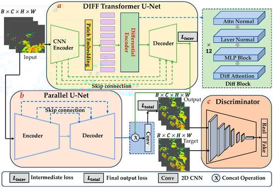
Figure 1.
The architecture of RaDiT module. (a) A hybrid DIFF transformer U-Net architecture where the encoder integrates three cascaded convolutional blocks and a differential transformer, and the decoder follows the up-sampling path of standard U-Net architecture. (b) A parallel U-Net generator that maintains symmetrical encoding–decoding operations throughout all spatial resolution stages. (c) A conditional GAN architecture discriminator that adversarially evaluates the authenticity of generated radar echo against targets.
| Algorithm 1 Discriminator Architecture |
| Require: Input tensor |
| Ensure: Validity probability |
| 1: Architecture Configuration: |
| 2: for do |
| 3: |
| 4: where |
| 5: end for |
| 6: Forward Process: |
| 7: forc cto 5 do |
| 8: |
| 9: end for |
| 10: |
| 11: |
| 12: return |
In summary, the key innovation of RaDiT is the first application of the DIFF transformer in radar echo prediction, which addresses the limitations of traditional Transformer architectures and significantly enhances performance in spatiotemporal forecasting tasks.
Additionally, a multi-level loss function is proposed, incorporating weighted loss components to guide model training in a hierarchical manner. This architecture combines intermediate supervision with terminal loss balancing, effectively enhancing the precise localization and intensity estimation of high-intensity echo regions.
2.2.2. Differential Attention of DIFF Transformer
Query, key, and value vectors are mapped to outputs using the differential attention [42] process. After computing attention scores using query and key vectors, we calculate a weighted sum of value vectors. Utilizing a pair of softmax functions to eliminate the noise in attention scores is a crucial design element. In particular, we first project them to query, key, and value , and given input . The outputs are then calculated using the differential attention operator employing
where are parameters, where represents the hidden dimension of the model, and is a learnable scalar. In order to synchronize the learning dynamics, we re-parameterize the scalar as
where is a constant used to initialize λ and are learnable vectors. Empirically, we discover that the configuration in Equation (4), in which stands for layer index, functions effectively in practice.
Analogous to differential amplifiers [47] proposed in electrical engineering, which use the difference between two signals as an output to null out the common-mode noise of the input. Subtracting the two softmax attention maps leverages differential weighting in attention mechanisms. The first map represents the general distribution of information, while the second one focuses on salient features, enhancing the signal. This subtraction highlights discrepancies between the maps, enabling the model to emphasize relevant parts of the input and suppress noise, typically characterized by inconsistencies or irrelevant information [41,42]. This method prioritizes meaningful patterns, reducing the influence of extraneous data that could hinder model performance.
The differential transformer also makes use of the multi-head mechanism [28]. Let h represent how many attention heads there are. For the heads, we employ various projection matrices . Within the same layer, heads share the scalar . Following normalization, the head outputs are projected to the end results as follows
where is a learnable projection matrix, employs RMSNorm [48] for every head, concatenates the heads together along the channel dimension, and is the constant scalar in Equation (3). To match the gradients with transformers, we utilize a fixed multiplier (1 − ) as the scale of . We determine the number of heads , where is transformer’s head dimension, to match the number of parameters and computational complexity.
The learnable scalar functions as a dynamic weighting factor, adjusting the relative importance of two attention maps. By learning the optimal value of , the model fine-tunes suppression and enhancement based on varying meteorological patterns. This adaptability allows the model to enhance relevant features in scenarios where specific atmospheric conditions, such as storms or cold fronts, dominate, improving performance in pattern recognition [36,42]. The matrix acts as a parameter that transforms the input space, enabling the attention mechanism to capture complex relationships between radar echoes more effectively [29,42].
The proposed architecture therefore implements a stack of L DIFF transformer layers (Figure 2), where each layer sequentially processes features through a multi-head differential attention mechanism followed by a feed-forward network module (Algorithm 2).
where is RMSNorm [48],
- ,
- are learnable matrices.
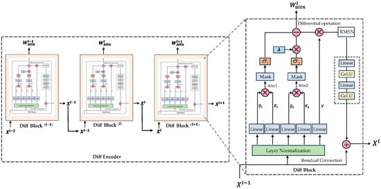
Figure 2.
Overall architecture of the differential encoder. The differential encoder comprises a total of layers. For an input X, the differential attention mechanism is iteratively computed times. Within each differential block, the operations attn1 and attn2 represent the first and second attention computations, respectively. Additionally, RMSN denotes RMSNorm.
| Algorithm 2 Differential Multi-Head Attention |
| Require: • Input tensor |
| • Weight matrices |
| • Output projection |
| • Balancing factor |
| • Number of heads |
| Ensure: Output tensor |
| 1: //——Single Head Differential Attention——DiffAttn |
| 2: Project inputs: |
| 3: Compute attention scores: |
| 4: return |
| 5: //——Multi-Head Composition—— |
| 6: Initialize output |
| 7: for head to do |
| 8: |
| 9: Apply normalization: |
| 10: Residual scaling: |
| 11: Collect heads: |
| 12: end for |
| 13: //——Final Projection—— |
| 14: Concatenate heads: |
| 15: Project output: |
2.3. Loss Function
2.3.1. Generator Loss Function
Two distinct loss functions are specifically designed for the generator of RaDiT to compute the intermediate loss of the model integrated with the DIFF transformer module and the final output loss . The intermediate loss function , which combines Structural Similarity Index Measure (SSIM) [49] and Mean Squared Error (MSE), is employed to calculate the frame-wise loss for the model incorporating the DIFF transformer module. The formulation of this loss function is defined as follows
where
- represents the predicted image, denotes the ground-truth image,
- is the total number of frames in the images.
and are introduced as learnable parameters to dynamically balance the contributions of the and terms within the hybrid loss function during model training.
- and are the mean intensities of and , respectively;
- and are variances of and , respectively;
- is covariance between and ;
- and are stabilization constants.
The final output loss integrates the Soft Dice Loss, Cross-Entropy Loss [50], and a Weighted Loss Function [51], which enhances the precision of radar echo reflectivity predictions by assigning higher weights to regions with intense echo signals. The formulation of the final output loss is defined as follows
where
- and are introduced as learnable parameters to dynamically balance the contributions of the and terms within the hybrid loss function during model training,
- is the continuous values of and , respectively;
- and denote the height and width of the radar echo images, respectively;
- and are the weight and the radar reflectivity at coordinate (, ), respectively.
This combined loss function ensures accurate prediction of radar echo reflectivity while emphasizing regions with higher echo intensity.
2.3.2. Discriminator Loss Function
The Binary Cross Entropy is adept as loss function of discriminator; the formulation of loss is defined as follows
where
- is predicted probability for the -th sample generated by the generator,
- is Ground truth label for the -th sample,
- is total number of samples in the dataset.
2.4. Evaluation Metrics
To comprehensively assess the performance of the RaDiT models, we adopt a multi-criteria evaluation strategy spanning predictive accuracy, spatiotemporal consistency, and probabilistic reliability, with additional metrics for event detection and bias analysis. Specifically, Fréchet Video Distance (FVD) [52,53] measures spatiotemporal consistency by comparing generated and real sequences; Continuous Ranked Probability Score (CRPS) [54] evaluates probabilistic reliability of forecasts; Critical Success Index (CSI), Probability of Detection (POD), and Equitable Threat Score (ETS) assess event detection capability for event detection. We also employ Peak Signal-to-Noise Ratio (PSNR) and Combined Reflectivity Absolute Error (CRAE) to evaluate the quality of the extrapolated echoes and assess the conservation of quality. Each metric evaluates distinct aspects of model performance, ensuring a robust multi-dimensional assessment. The mathematical formulations and interpretations are defined as follows:
- : Quantifies similarity between predicted and ground-truth radar echo sequences by comparing their feature distributions in a latent space, where and are mean feature vectors, and , are covariance matrices. This metric is particularly effective for evaluating temporal consistency.
- : Measures the accuracy of probabilistic forecasts by integrating the squared difference between predicted and observed cumulative distribution functions (CDFs), where is the predicted CDF, and is the ground-truth CDF.
- To the Classification Metrics , , , whereTrue Positives (): Correctly predicted events.False Positives (): Incorrectly predicted events (predicted but not observed).False Negatives (): Missed events (observed but not predicted).True Negatives (): Cases where the model correctly predicts the absence of an event when no event is observed.
- : Measures the quality of extrapolated echoes, where denotes the maximum possible pixel value of the image.
- : Assesses the conservation of quality by calculating the absolute error between the extrapolated radar echo results for each frame and the ground truth, based on the accumulated values within the threshold region. Here, is an indicator function, where if the condition is satisfied, and otherwise. is a threshold used to filter which echo values should be included in the calculation.
Following [26], we evaluate perceptual quality by computing , , and at 4 × 4 and 16 × 16 pooling scales. This multi-scale approach assesses the model’s ability to predict radar echo reflectivity across spatial aggregations, revealing performance variations at local (4 × 4) and regional (16 × 16) resolutions. Average pooling is applied to predicted and ground-truth maps before thresholding and metric calculation, ensuring robustness to spatial variability.
2.5. Implementation Details
The RaDiT framework is implemented in PyTorch v2.4, with distinct hardware configurations for different datasets. CMARC data processing employs dual NVIDIA A100 GPUs with a 32-sample batch size, while SEVIR dataset training utilizes a single NVIDIA RTX 4090 GPU maintaining the same batch size. The architecture processes temporal sequences of 16 consecutive frames (6 min temporal resolution) to predict 16 subsequent frames for the CMARC applications, and 6-frame inputs (10 min temporal resolution) to forecast 6 subsequent frames for SEVIR data. The detailed adversarial training procedure for the RaDiT model is presented in Algorithm 3.
| Algorithm 3 Adversarial Training Strategy |
| Require: • Generator , Discriminator |
| •Training dataset |
| •Loss functions: |
| •Hyperparameters: |
| Ensure: Optimized parameters: |
| 1: Initialize gradients: |
| 2: for epoch = 1 to do |
| 3: for batch do |
| 4: //--Generator Forward--// |
| 5: |
| 6: //--Discriminator Phase 1--// |
| 7: |
| 8: |
| 9: |
| 10: //--Generator Optimization--// |
| 11: |
| 12: |
| 13: |
| 14: //--Discriminator Phase 2--// |
| 15: |
| 16: |
| 17: |
| 18: if batch then |
| 19: |
| 20: {Reset accumulated gradients} |
| 21: end if |
| 22: end for |
| 23: end for |
Training employs the AdamW optimizer with an initial learning rate of 1 × 10⁻⁴, weight decay 1 × 10⁻³, continuing for up to 1000 epochs. Convergence optimization integrates early stopping with a 50-epoch patience period and cosine annealing learning rate scheduling with a 100-cycle period. The ViT component implements the ViT-B16 architecture [29], configured with 12 transformer layers and 768-dimensional embeddings (K = 768), processing input through 16 × 16 spatial patches. All models initialize without pre-trained weights to ensure baseline comparability.
For the CMARC benchmarks, identical training protocols (batch size = 32, AdamW optimizer, initial LR = 1 × 10⁻⁴, weight decay 1 × 10⁻³, 1000-epoch maximum, cosine annealing learning rate scheduling with a 100-cycle period) are applied to eight comparative models: ConvLSTM [21], PredRNN [22], U-Net [12], TAU [37], UNETR [50], UNETR++ [55], PhyDNet [56], and PreDiff [26]. This standardized evaluation protocol ensures equitable performance comparison across all architectures while maintaining dataset-specific computational resource allocations.
During testing, the trained model predicts future frames based on input temporal sequences. For CMARC, the model predicts 16 subsequent frames from a 16-frame input sequence (6 min temporal resolution). For SEVIR, the model forecasts 6 subsequent frames from 6-frame inputs (10 min temporal resolution). The output is then compared to the ground truth, and evaluation metrics are calculated. In addition to testing the RaDiT framework, we also evaluated the performance of eight baseline models using the same test set, evaluation metrics, and testing protocol. This ensures that all models are tested under identical conditions for a fair comparison.
3. Results
3.1. SEVIR VIL Extrapolation
In this section, we first conduct a quantitative evaluation of the RaDiT model using VIL data from the publicly available SEVIR dataset, accompanied by perceptual quality analysis. Subsequently, an ablation study is performed to systematically examine the impact of individual model components on the perceptual outcomes.
3.1.1. Comparison with the State of the Art
We conduct experiments using the VIL product from the SEVIR dataset, where both RaDiT and baseline models employ 6-frame inputs (10 min temporal resolution) to predict 6 subsequent frames. Additionally, we refine the Weighted Loss Function [51] to accommodate the stratified nature of the VIL data. The PreDiff model [26], along with comparative models including U-Net, ConvLSTM, PredRNN, PhyDNet, E3D-LSTM [57], Rainformer [58], Earthformer [59], VideoGPT [60], and LDM [61], are evaluated using results from their respective original publications.
As shown in Table 1, the DIFF-transformer-based model RaDiT demonstrates superior ability to capture spatiotemporal patterns and the true data distribution. It achieves significantly high FVD scores and notably improved CSI metrics at both 4 × 4 (CSI-pool4) and 16 × 16 (CSI-pool16) pooling resolutions, without a significant increase in the model’s parameters. For VIL values exceeding the thresholds [133, 160, 181, 219], the average CSI improvements are observed to be 16.67% and 6.52% compared to the state-of-the-art PreDiff at spatial pooling scales of 4 and 16, respectively.

Table 1.
The comparison of model parameters and performance comparison on the SEVIR dataset. The CSI is computed at multiple VIL intensity thresholds (denoted as CSI-thresh). CSI represents the average of CSI values at thresholds [16, 74, 133, 160, 181, 219] over extended lead times. CSI-pool metrics (s = 4 and s = 16) indicate spatial pooling scales of 4 × 4 and 16 × 16, respectively. Additionally, we evaluate probabilistic forecasting performance using the CRPS and quantify visual coherence through the FVD.
Although RaDiT exhibits less optimization for pixel-level metrics, it demonstrates enhanced capability in capturing localized data distributions, achieving higher CSI at 16 × 16 pooling (CSI-pool16), low CRPS, and preserving spatially coherent structures. Furthermore, Table 2 and Table 3 present that the integration of the Weighted Loss Function during training significantly improves model performance under elevated threshold conditions.
Table 2.
CSI-pool4 at thresholds [16, 74, 133, 160, 181, 219] on SEVIR.
Table 3.
CSI-pool16 at thresholds [16, 74, 133, 160, 181, 219] on SEVIR.
3.1.2. Ablation Study on SEVIR
To assess the individual contributions of the DIFF transformer and GAN modules, we perform ablation studies to examine their effects on model performance. Table 2 presents quantitative comparisons of four model variants: (1) RaDiT without GAN—where adversarial training is removed, and the generator directly produces the outputs; (2) RaDiT without GAN and DIFF—a simplified version that retains only the standard transformer module; (3) RaDiT without DIFF—a hybrid architecture combining conventional transformers with GAN-based adversarial training; and (4) the full RaDiT model. Notably, the role of Weighted Loss Function has been established in [51], and the same loss function is applied in all experiments, so we do not discuss it separately. Furthermore, we provide a comparative evaluation of VIL prediction performance at varying thresholds using metrics such as CSI, POD, and ETS, as shown in Figure 3.
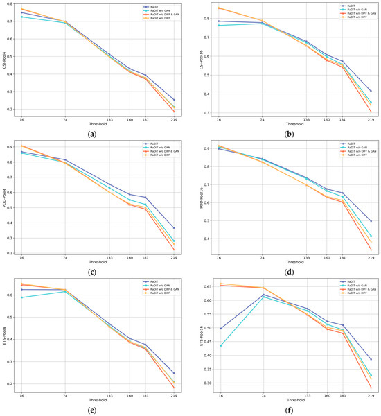
Figure 3.
Performance comparison of event detection metrics under varying thresholds for 4 × 4 and 16 × 16 pooling configurations in ablation studies: (a,b) CSI, (c,d) POD, (e,f) ETS.
This multi-threshold analysis enables systematic assessment of module contributions by examining prediction accuracy across distinct VIL intensity levels. For enhanced interpretability, Figure 4 provides visual comparisons of extrapolation results across these configurations.
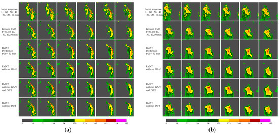
Figure 4.
Comparative visualization of ablation study results. Input sequences span −60~−10 min at 10 min temporal resolution, with the model predicting VIL spatiotemporal features for 0–50 min. (a) Performance evaluation of VIL predictions during a squall line event; (b) comparative analysis of VIL evolution dynamics under developmental conditions.
As can be seen from Table 4, models incorporating the DIFF transformer module consistently achieve higher threshold-average scores. Surprisingly, RaDiT, when enhanced with the DIFF transformer architecture, demonstrates statistically significant performance improvements through GAN integration. Further analysis revealed that models utilizing conventional transformer architectures experience a noticeable decline in evaluation scores, regardless of whether they are integrated with the GAN.
Table 4.
Ablation study results on SEVIR.
Meanwhile, as demonstrated in Figure 3, models integrating the DIFF transformer module achieve superior CSI, POD, and ETS across varying VIL thresholds for both 4 × 4 and 16 × 16 pooling configurations. Figure 4 further reveals that the DIFF transformer-enhanced model demonstrates enhanced spatiotemporal consistency in extrapolating VIL patterns, with its predictions progressively aligning closer to ground truth observations as the forecast horizon extends.
3.1.3. Ablation Study of on SEVIR
Due to the empirical nature of the scheme, we conducted sensitivity experiments to verify and identify the optimal lambda configuration. Table 5 presents six sets of ablation experiments related to : (1) _ ours—inherits the empirical design of the DIFF transformer; (2) _ constant--the scheme is constant; (3) _exponent—the scheme follows an exponential function; (4) _logarithm—the scheme follows a logarithmic function; (5) _ square root—the scheme follows a square root function; (6) _inverse proportionality—the scheme follows an inverse proportionality function. All scheme designs ensure that the values of lambda meet the requirements of the DIFF transformer module. The metrics used are consistent with the CSI outlined in Section 3.1.2.
Table 5.
Ablation study results of on SEVIR.
As shown in Table 5, the DIFF transformer module with _ ours consistently achieves higher threshold-average scores. The _ inverse proportionality scheme results in the lowest threshold-average scores, primarily because the inverse proportionality function decreases asymptotically towards zero as increases. Additionally, the constant scheme yields the second-lowest scores, indicating that using the same for different values of is disadvantageous, as it prevents the model from effectively adapting to these variations.
3.2. CMARC Echo Extrapolation
In this section, we present a quantitative assessment of the RaDiT model on the CMARC dataset, combined with a perceptual quality analysis to evaluate visual fidelity. Following this, we perform a comprehensive ablation study to rigorously investigate the influence of distinct architectural components on the perceptual performance.
3.2.1. Experimental Setup
In this study, experiments are performed using radar reflectivity products from the CMARC dataset. Both the RaDiT and comparative models utilize 16-frame input sequences (6 min temporal resolution) to predict 16 subsequent frames. Notably, the CMARC data undergoes only standard quality control and normalization procedures, without any clustering applied to discrete or low-magnitude echoes [21]. This approach helps maintain the inherent distribution characteristics of the dataset. Furthermore, the Weighted Loss Function (Equation (17)) [51] is implemented to address the stratified structure of the CMARC data. To ensure a fair performance comparison, comparative models including ConvLSTM, PredRNN, TAU, U-Net, UNETR, UNETR++, PhyDNet, and PreDiff are implemented using the open-source code specified in their original publications and trained with the identical strategy employed for RaDiT.
3.2.2. Experimental Results
We utilize the full test dataset of the CMARC benchmark to evaluate model performance and compute standard evaluation metrics. Table 6 presents the average metric values across intensity thresholds [15, 20, 25, 30, 35, 40, 45, 50, 60] for our proposed model, in comparison to the performance of other models. Figure 5 further illustrates comparative analyses of CSI, POD, and ETS metrics under 4 × 4 and 16 × 16 spatial pooling resolutions. Additionally, Figure 6, Figure 7, Figure 8 and Figure 9 demonstrate four representative cases of intense convective events, providing visual comparisons between our method and alternative approaches. The experimental findings reveal the following key observations:
Table 6.
The comparison of model parameters, iteration time, and performance on the CMARC dataset. The CSI is computed at multiple echo intensity thresholds (denoted as CSI-thresh). CSI represents the average of CSI values at thresholds [15, 20, 25, 30, 35, 40, 45, 50, 60]. CSI-pool metrics (s = 4 and s = 16) indicate spatial pooling scales of 4 × 4 and 16 × 16, respectively.
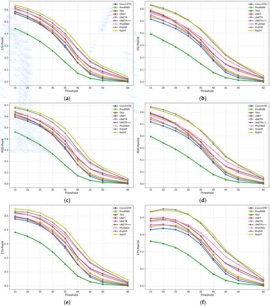
Figure 5.
Performance comparison of event detection metrics under varying thresholds [15, 20, 25, 30, 35, 40, 45, 50, 60] for 4 × 4 and 16 × 16 pooling configurations in comparative models: (a,b) CSI, (c,d) POD, (e,f) ETS.
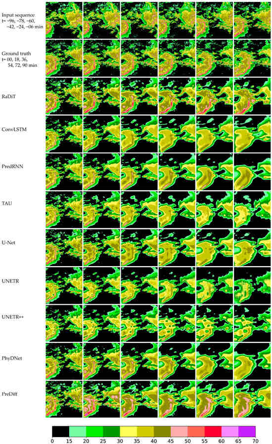
Figure 6.
Comparison of a squall line system associated with eastward-migrating Southwest China Vortex in Jiangxi Province (29 April 2024, 15:00–18:06 UTC). (Row 1) Radar reflectivity inputs at 15:00, 15:18, 15:36, 15:54, 16:12, and 16:30. (Row 2) Ground-truth observations at 16:36, 16:54, 17:12, 17:30, 17:48, and 18:06. (Subsequent rows) Prediction results from the proposed RaDiT model and ConvLSTM, PredRNN, TAU, U-Net, UNETR, UNETR++, PhyDNet, PreDiff, demonstrating spatiotemporal extrapolation performance under complex convective weather conditions.
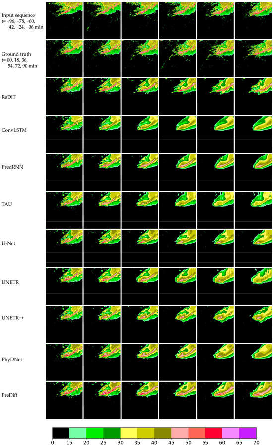
Figure 7.
Comparative experimental results of a cold air mass-triggered squall line system from 06:00 to 09:06 (UTC) on 4 April 2024, in the Pearl River Delta region. (Row 1) Radar reflectivity inputs at 06:00, 06:18, 06:36, 06:54, 07:12 and 07:30. (Row 2) Ground-truth observations at 07:36, 07:54, 08:12, 08:30, 08:48 and 09:06.
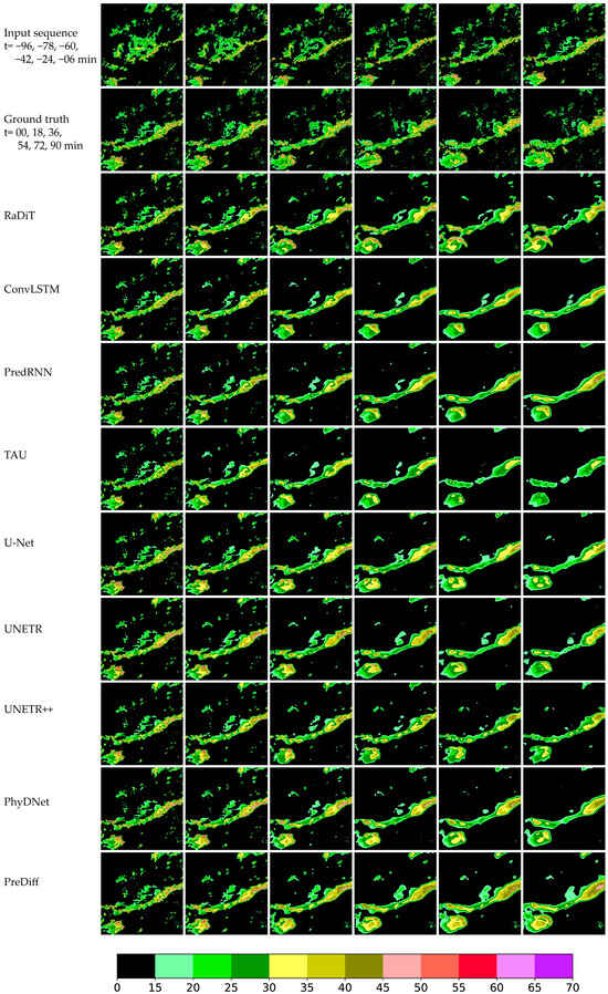
Figure 8.
Comparative experimental results of a cold front process from 06:00 to 09:06 (UTC) on 22 June 2024, in Guizhou Province. (Row 1) Radar reflectivity inputs at 06:00, 06:18, 06:36, 06:54, 07:12 and 07:30. (Row 2) Ground-truth observations at 07:36, 07:54, 08:12, 08:30, 08:48 and 09:06.
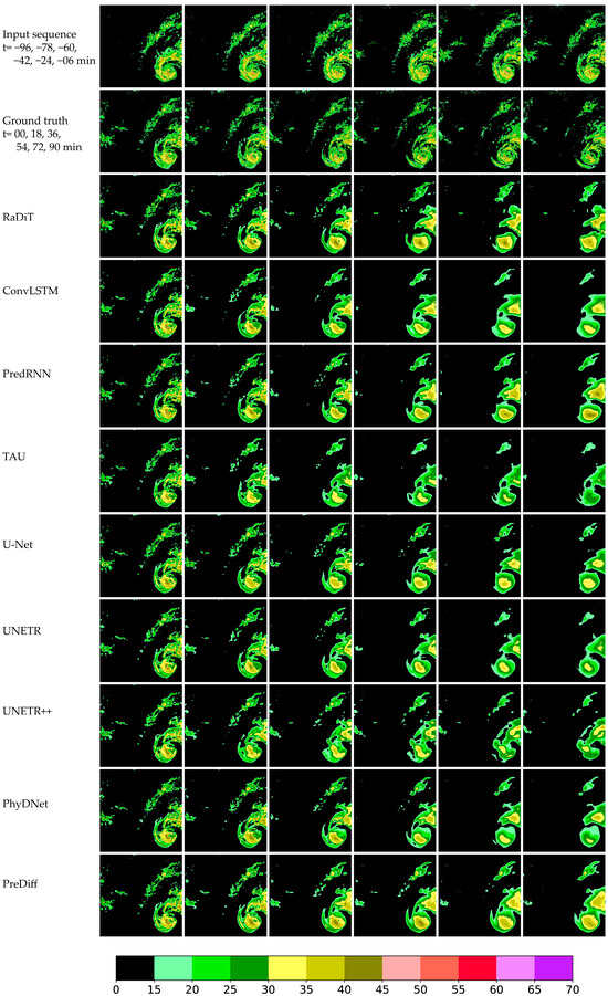
Figure 9.
Comparative experimental results of Super Typhoon Koinu (International ID: 2314) from 10:00 to 13:06 (UTC) on 7 October 2023, in the Pearl River Delta Region. (Row 1) Radar reflectivity inputs at 10:00, 10:18, 10:36, 10:54, 11:12 and 11:30. (Row 2) Ground-truth observations at 11:36, 11:54, 11:12, 11:30, 11:48 and 11:06.
The proposed model demonstrates superior performance in extrapolating strong radar echoes compared to existing methods. Quantitative analysis reveals that RaDiT achieves the highest average CSI and POD scores across thresholds [15, 20, 25, 30, 35, 40, 45, 50, 60]. As shown in Figure 5, RaDiT also attains peak scores for CSI, POD, and ETS metrics under both 4 × 4 and 16 × 16 spatial pooling scales, particularly at thresholds exceeding 30 dBZ, without a significant increase in model parameters and iteration time (Table 6). Further analysis of Experimental results reveals that when composite radar reflectivity exceeds critical thresholds [30, 35, 40, 45, 50, 60], RaDiT achieves average CSI improvements of 10.23% and 2.88% compared to the state-of-the-art PreDiff at spatial pooling scales of 4 × 4 and 16 × 16, respectively.
Furthermore, Figure 6, Figure 7, Figure 8 and Figure 9 demonstrate that the RaDiT model exhibits superior spatial morphology preservation in extrapolating intense convective echoes, particularly for reflectivity values exceeding 50 dBZ. Comparative analysis reveals that all benchmark models except PreDiff systematically underestimate echo intensity, with this underestimation becoming pronounced beyond the 54 min forecast lead time. Notably, competing models fail to extrapolate echoes above 50 dBZ at the 90 min prediction horizon. The most striking result from the data is that, while PreDiff demonstrates competitive performance, RaDiT exhibits a closer alignment with ground truth observations in three key aspects—echo intensity maintenance, morphological consistency, and spatial positioning accuracy—across all forecast lead times.
In conclusion, the proposed RaDiT model demonstrates superior performance in forecasting both spatial positioning details and high-reflectivity regions over extended lead times compared to benchmark methods. This capability highlights its effectiveness in maintaining spatiotemporal consistency and prediction accuracy for critical meteorological phenomena.
3.2.3. Ablation Study on CMARC
Ablation studies are conducted to evaluate the individual contributions of key components to model performance on the CMARC datasets. As summarized in Table 7, four model variants are quantitatively compared: (1) RaDiT w/o GAN, a configuration eliminating adversarial training and generating outputs directly from the generator; (2) RaDiT w/o GAN and DIFF, a streamlined variant preserving only the standard transformer module; (3) RaDiT w/o DIFF, a hybrid framework integrating conventional transformers with GAN-based adversarial training; and (4) the complete RaDiT architecture incorporating all proposed components. This systematic evaluation isolates the performance impacts of adversarial learning mechanisms and the DIFF transformer module while maintaining consistency in experimental conditions. Notably, the role of Weighted Loss Function has been established in [51], and the same loss function is applied in all experiments, so we do not discuss it separately.
Table 7.
Ablation study results on the CMARC dataset.
As quantified in Table 6, models integrating the DIFF transformer module demonstrate consistent superiority in threshold-averaged evaluation metrics. Specifically, the GAN-enhanced RaDiT variant equipped with the DIFF transformer architecture exhibits statistically significant enhancements in predictive accuracy, highlighting the complementary relationship between adversarial training and the spatiotemporal feature extraction capabilities of the DIFF transformer module. In contrast, implementations utilizing traditional transformer designs experience measurable performance degradation when combined with GAN.
In summary, these results are consistent with observations from the SEVIR dataset, validating the DIFF transformer’s ability to generalize and efficiently extract relevant information from long-range spatiotemporal dependencies for radar extrapolation tasks.
4. Discussion
For radar extrapolation tasks derived from complex spatiotemporal Earth observation systems, traditional methods often face significant challenges. These include the inability to adequately represent spatiotemporal interactions in rapidly evolving convective processes and the suboptimal utilization of features in extended radar echo sequences. As a result, these methods tend to produce overly smooth predictions, compensating for deficiencies in quantitative performance metrics. Specifically, they exhibit systematic biases in both the estimation of intensity and the spatial localization of strong echo signatures.
To overcome these challenges, the RaDiT framework introduces advanced architecture featuring a DIFF transformer variant, which exhibits enhanced predictive performance in radar extrapolation tasks, as detailed in Section 3. While the self-attention mechanism [36,37,38] is effective in capturing correlations within input data, it can also introduce irrelevant noise, particularly in long temporal sequences. In radar echo extrapolation tasks, echo evolution typically involves strong spatiotemporal dependencies. However, certain time points may introduce background noise that is unrelated to the target echo. The DIFF transformer addresses this by filtering out such irrelevant information and focusing on key temporal patterns, thereby improving the signal-to-noise ratio (Figure 10a). This approach strengthens the model’s ability to focus on relevant features, facilitating the capture of radar echo evolution patterns. As shown in Section 3, extensive experiments highlight the effectiveness of the differential attention mechanism in minimizing unrelated attention, enabling the model to better identify core patterns within weather systems. In particular, during the spatiotemporal evolution process, this mechanism excels at identifying critical weather changes [62], while also adhering to the physical constraint of mass conservation (Figure 10b). Overall, the system leverages differential attention mechanisms to achieve three key improvements: the suppression of attention noise artifacts in spatiotemporal predictions, robust modeling of long-range dependencies, and a substantial reduction in the generation of extraneous features.
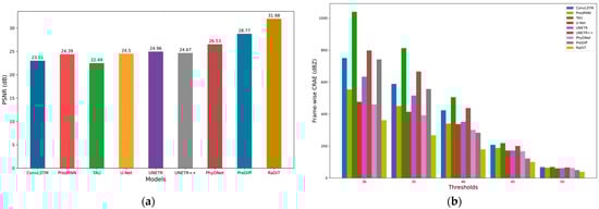
Figure 10.
Comparative experimental results of PSNR (a) and frame-wise CRAE between the threshold-based combined reflectance extrapolation results and ground truth (b) from the proposed RaDiT model, along with ConvLSTM, PredRNN, TAU, U-Net, UNETR, UNETR++, PhyDNet, and PreDiff, are presented on the entire CMARC test set.
Furthermore, the framework integrates Weighted Loss Functions [51] to prioritize strong echo patterns during model training, combined with adversarial training via the GAN module to enhance the spatial fidelity of the predictions. This dual-strategy approach not only improves the accuracy of feature representation but also preserves critical spatial details that are often lost due to excessive smoothing in models such as ConvLSTM, PredRNN and U-Net. Notably, this architectural design specifically addresses spatial displacement errors in high-intensity regions, achieving average ≥30dBZ CSI improvements of 10.23% and 2.88% on CMARC dataset compared to the state-of-the-art PreDiff at spatial pooling scales of 4 × 4 and 16 × 16, respectively.
Experimental validation on benchmark datasets (SEVIR and CMARC) demonstrates that, while RaDiT shows slightly lower optimization for conventional pixel-level metrics, it excels in capturing localized data distributions, achieving improved perceptual scores, and maintaining spatially coherent structural patterns across different climatic regions and weather systems (Figure 6, Figure 7, Figure 8 and Figure 9). RaDiT also demonstrates strong performance in radar echo extrapolation across various radar models, polarization types, and weather systems, indicating that the model exhibits excellent robustness and generalization capabilities. These capabilities are particularly critical for the precise identification of meteorological events, especially in operational applications that require high-accuracy spatial localization of atmospheric processes [63]. This includes, but is not limited to, extreme weather monitoring, convective system tracking, and mesoscale climate dynamics analysis.
Further analysis, including systematic ablation studies, confirms the functional contributions of the DIFF transformer and GAN modules, leading to three key findings:
- Enhanced Pattern Capture and Noise Suppression with Attention Mechanisms
Models incorporating the DIFF transformer module exhibit superior performance in capturing radar echo evolution patterns, with notable improvements in event detection metrics, including CSI-Pool4 and CSI-Pool6 scores (Table 2, Table 3 and Table 5). When trained with weighted loss strategies, these models exhibit enhanced noise suppression under high-threshold conditions. For VIL values exceeding thresholds of [133, 160, 181, 219], average CSI improvements of 16.67% and 6.52% are observed on the SEVIR dataset compared to the state-of-the-art PreDiff at spatial pooling scales of 4 and 16, respectively. This effectively minimizes the generation of spurious features and enhances the reliability of the metrics.
- Precision in Critical Feature Localization
DIFF-transformer-enhanced variants consistently achieve POD and ETS values (Figure 3 and Figure 5) approaching the optimal threshold across both SEVIR and CMARC datasets. This indicates their improved capability to accurately localize high-intensity meteorological features and maintain spatial precision in complex spatiotemporal prediction tasks.
- Perceptual Quality and Structural Fidelity
The integration of DIFF transformer significantly improves perceptual scores and structural coherence in the predictions. While the module itself enhances atmospheric field representation, the addition of GAN further refines fine-scale details, resulting in better alignment with ground-truth observations in both spatial patterns and intensity distributions (Figure 10). Notably, only models with the DIFF transformer accurately capture the spatial positioning and developmental trajectories of high-intensity echoes, a critical capability for applications requiring precise tracking of rapidly evolving weather systems.
In summary, the combined architecture effectively addresses the ongoing challenge of inadequately representing spatiotemporal interactions in rapidly evolving convective processes, as well as the suboptimal utilization of features in extended radar echo sequences. The DIFF transformer enables scale-aware feature representation, while the GAN module enhances fine details through a synergistic interaction, ultimately improving the operational utility of radar echo extrapolation frameworks.
5. Conclusions
This paper introduces the differential transformer, a novel architecture that enhances the ability to amplify contextually relevant patterns while effectively suppressing noise interference in large language models. We employ this mechanism as the core encoder to develop RaDiT, an efficient spatiotemporal prediction framework specifically optimized for radar echo extrapolation tasks. Extensive experimental evaluations demonstrate that RaDiT achieves unparalleled performance in radar echo extrapolation, outperforming existing models across multiple evaluation metrics, while also demonstrating strong robustness and generalization capabilities. The framework exhibits superior effectiveness and accuracy in processing high-intensity echo regions compared to other models. This study represents the first implementation of DIFF transformer architectures for radar echo extrapolation in meteorological applications. While demonstrating superior performance on benchmark radar datasets, this study has not yet validated the framework’s generalizability across multi-sensor Earth observation scenarios, particularly those involving dual-polarization radar configurations or synergistic satellite–radar data fusion. Future work will explore new research directions for integrating differential mechanisms with attention-based architectures, especially for processing high-dimensional and multi-sensor Earth observation data, where simultaneous noise suppression and detail preservation are critical.
Author Contributions
Conceptualization, W.Z.; methodology, W.Z.; software, W.Z.; validation, W.Z. and Z.Z.; formal analysis, W.Z.; investigation, W.Z. and Y.Z.; resources, Z.L.; data curation, W.Z. and R.L.; writing—original draft preparation, W.Z.; writing—review and editing, B.L.; visualization, W.Z. and Y.Z.; supervision, Z.L.; project administration, Z.L.; funding acquisition, Z.L. All authors have read and agreed to the published version of the manuscript.
Funding
This research was funded by the Joint Fund of Zhejiang Provincial Natural Science Foundation of China, grant number LZJMD25D050002.
Data Availability Statement
The Storm Event Imagery (SEVIR) dataset can be downloaded from this address: https://registry.opendata.aws/sevir/, accessed on 20 September 2024. The CMA radar reflectivity (CMARC) data, collected from the national radar composite network developed by the Atmospheric Detection Center of the China Meteorological Administration is unavailable due to privacy.
Conflicts of Interest
The authors declare no conflicts of interest.
References
- Weisman, M.L.; Klemp, J.B. The dependence of numerically simulated convective storms on vertical wind shear and buoyancy. Mon. Weather Rev. 1982, 110, 504–520. [Google Scholar] [CrossRef]
- Imhoff, R.O.; Brauer, C.C.; Overeem, A.; Weerts, A.H.; Uijlenhoet, R. Spatial and temporal evaluation of radar rainfall nowcasting techniques on 1533 events. Water Resour. Res. 2020, 56, e2019WR026723. [Google Scholar] [CrossRef]
- Dixon, M.; Wiener, G. TITAN: Thunderstorm Identification, Tracking, Analysis, and Nowcasting—A Radar-Based Methodology. J. Atmos. Ocean. Technol. 1993, 10, 785–797. [Google Scholar] [CrossRef]
- Zhang, C.; Zhou, X.; Zhuge, X.; Xu, M. Learnable Optical Flow Network for Radar Echo Extrapolation. IEEE J. Sel. Top. Appl. Earth Obs. Remote Sens. 2021, 14, 1260–1266. [Google Scholar] [CrossRef]
- Ayzel, G.; Heistermann, M.; Winterrath, T. Optical Flow Models as an Open Benchmark for Radar-Based Precipitation Nowcasting (Rainymotion v0.1). Geosci. Model Dev. 2019, 12, 1387–1402. [Google Scholar] [CrossRef]
- Mai, X.; Zhong, H.; Li, L. Using SVM to Provide Precipitation Nowcasting Based on Radar Data. In Advances in Natural Computation, Fuzzy Systems and Knowledge Discovery. ICNC-FSKD 2019; Liu, Y., Wang, L., Zhao, L., Yu, Z., Eds.; Advances in Intelligent Systems and Computing; Springer: Cham, Switzerland, 2020; Volume 1075. [Google Scholar] [CrossRef]
- Yu, P.; Yang, T.; Chen, S.; Kuo, C.; Tseng, H. Comparison of Random Forests and Support Vector Machine for Real-Time Radar-Derived Rainfall Forecasting. J. Hydrol. 2017, 552, 92–104. [Google Scholar] [CrossRef]
- Yang, Z.; Liu, P.; Yang, Y. Convective/Stratiform Precipitation Classification Using Ground-Based Doppler Radar Data Based on the K-Nearest Neighbor Algorithm. Remote Sens. 2019, 11, 2277. [Google Scholar] [CrossRef]
- Aderyani, F.R.; Mousavi, S.J.; Jafari, F. Short-Term Rainfall Forecasting Using Machine Learning-Based Approaches of PSO-SVR, LSTM, and CNN. J. Hydrol. 2022, 614, 128463. [Google Scholar] [CrossRef]
- Ronneberger, O.; Fischer, P.; Brox, T. U-Net: Convolutional Networks for Biomedical Image Segmentation. In Medical Image Computing and Computer-Assisted Intervention—MICCAI 2015; Navab, N., Hornegger, J., Wells, W., Frangi, A., Eds.; MICCAI 2015, Lecture Notes in Computer Science; Springer: Cham, Switzerland, 2015; Volume 9351, pp. 234–241. [Google Scholar] [CrossRef]
- Chen, J.; Lu, Y.; Yu, Q.; Luo, X.; Adeli, E.; Wang, Y.; Lu, L.; Yuille, A.L.; Zhou, Y. TransUNet: Transformers Make Strong Encoders for Medical Image Segmentation. arXiv 2021, arXiv:2102.04306. [Google Scholar] [CrossRef]
- Çiçek, Ö.; Abdulkadir, A.; Lienkamp, S.S.; Brox, T.; Ronneberger, O. 3D U-Net: Learning Dense Volumetric Segmentation from Sparse Annotation. In Medical Image Computing and Computer-Assisted Intervention—MICCAI 2016; Ourselin, S., Joskowicz, L., Sabuncu, M., Unal, G., Wells, W., Eds.; MICCAI 2016, Lecture Notes in Computer Science; Springer: Cham, Switzerland, 2016; Volume 9901, pp. 424–432. [Google Scholar] [CrossRef]
- Han, L.; Liang, H.; Chen, H.; Zhang, W.; Ge, Y. Convective Precipitation Nowcasting Using U-Net Model. IEEE Trans. Geosci. Remote Sens. 2022, 60, 4103508. [Google Scholar] [CrossRef]
- Zhou, K.; Zheng, Y.; Dong, W.; Wang, T. A Deep Learning Network for Cloud-to-Ground Lightning Nowcasting with Multisource Data. J. Atmos. Ocean. Technol. 2020, 37, 927–942. [Google Scholar] [CrossRef]
- Leinonen, J.; Hamann, U.; Germann, U. Seamless Lightning Nowcasting with Recurrent-Convolutional Deep Learning. Artif. Intell. Earth Syst. 2022, 1, 1–46. [Google Scholar] [CrossRef]
- Bengio, Y.; Simard, P.; Frasconi, P. Learning Long-Term Dependencies with Gradient Descent Is Difficult. IEEE Trans. Neural Netw. 1994, 5, 157–166. [Google Scholar] [CrossRef] [PubMed]
- Pascanu, R.; Mikolov, T.; Bengio, Y. On the Difficulty of Training Recurrent Neural Networks. In Proceedings of the 30th International Conference on Machine Learning, PMLR, Atlanta, GA, USA, 16–21 June 2013; Available online: https://proceedings.mlr.press/v28/pascanu13.html (accessed on 24 October 2024).
- Hochreiter, S.; Schmidhuber, J. Long Short-Term Memory. Neural Comput. 1997, 9, 1735–1780. [Google Scholar] [CrossRef] [PubMed]
- Salem, F. Gated RNN: The Gated Recurrent Unit (GRU) RNN. In Recurrent Neural Networks; Springer: Cham, Switzerland, 2022. [Google Scholar] [CrossRef]
- Liu, H.; Liu, C.; Wang, J.T.L.; Wang, H. Predicting Solar Flares Using a Long Short-Term Memory Network. Astrophys. J. 2019, 877, 121. [Google Scholar] [CrossRef]
- Shi, X.; Chen, Z.; Wang, H.; Yeung, D.-Y.; Wong, W.-k.; Woo, W.-c. Convolutional LSTM Network: A Machine Learning Approach for Precipitation Nowcasting. In Proceedings of the 29th International Conference on Neural Information Processing Systems—Volume 1, Montreal, QC, Canada, 7–12 December 2015; MIT Press: Cambridge, MA, USA, 2015; pp. 802–810. [Google Scholar]
- Wang, Y.; Long, M.; Wang, J.; Gao, Z.; Yu, P.S. PredRNN: Recurrent Neural Networks for Predictive Learning Using Spatiotemporal LSTMs. In Proceedings of the 31st International Conference on Neural Information Processing Systems, Long Beach, CA, USA, 4–9 December 2017; Curran Associates Inc.: Red Hook, NY, USA, 2017; pp. 879–888. [Google Scholar]
- Wang, Y.; Wu, H.; Zhang, J.; Gao, Z.; Wang, J.; Yu, P.S.; Long, M. PredRNN: A Recurrent Neural Network for Spatiotemporal Predictive Learning. IEEE Trans. Pattern Anal. Mach. Intell. 2023, 45, 2208–2225. [Google Scholar] [CrossRef]
- Zhong, S.; Zeng, X.; Ling, Q.; Wen, Q.; Meng, W.; Feng, Y. Spatiotemporal Convolutional LSTM for Radar Echo Extrapolation. In Proceedings of the 2020 54th Asilomar Conference on Signals, Systems, and Computers, Pacific Grove, CA, USA, 1–5 November 2020; IEEE: Piscataway, NJ, USA, 2020; pp. 58–62. [Google Scholar] [CrossRef]
- Zheng, K.; Liu, Y.; Zhang, J.; Luo, C.; Tang, S.; Ruan, H.; Tan, Q.; Yi, Y.; Ran, X. GAN-argcPredNet v1.0: A Generative Adversarial Model for Radar Echo Extrapolation Based on Convolutional Recurrent Units. Geosci. Model Dev. 2022, 15, 1467–1475. [Google Scholar] [CrossRef]
- Gao, Z.; Shi, X.; Han, B.; Wang, H.; Jin, X.; Maddix, D.; Zhu, Y.; Li, M.; Wang, Y. PreDiff: Precipitation Nowcasting with Latent Diffusion Models. In Proceedings of the 37th International Conference on Neural Information Processing Systems, Orleans, LA, USA, 10–16 December 2023; Curran Associates Inc.: Red Hook, NY, USA, 2023; pp. 1–36. [Google Scholar]
- Liu, Q.; Yang, Z.; Ji, R.; Zhang, Y.; Bilal, M.; Liu, X.; Vimal, S.; Xu, X. Deep Vision in Analysis and Recognition of Radar Data: Achievements, Advancements, and Challenges. IEEE Syst. Man Cybern. Mag. 2023, 9, 4–12. [Google Scholar] [CrossRef]
- Vaswani, A.; Shazeer, N.; Parmar, N.; Uszkoreit, J.; Jones, L.; Gomez, A.N.; Kaiser, L.; Polosukhin, I. Attention Is All You Need. arXiv 2017, arXiv:1706.03762. [Google Scholar] [CrossRef]
- Dosovitskiy, A.; Beyer, L.; Kolesnikov, A.; Weissenborn, D.; Zhai, X.; Unterthiner, T.; Dehghani, M.; Minderer, M.; Heigold, G.; Gelly, S.; et al. An Image is Worth 16 × 16 Words: Transformers for Image Recognition at Scale. arXiv 2020, arXiv:2010.11929. [Google Scholar] [CrossRef]
- Aleissaee, A.A.; Kumar, A.; Anwer, R.M.; Khan, S.; Cholakkal, H.; Xia, G.-S.; Khan, F.S. Transformers in Remote Sensing: A Survey. Remote Sens. 2023, 15, 1860. [Google Scholar] [CrossRef]
- Bi, K.; Xie, L.; Zhang, H.; Chen, X.; Gu, X.; Tian, Q. Accurate medium-range global weather forecasting with 3D neural networks. Nature 2023, 619, 533–538. [Google Scholar] [CrossRef] [PubMed]
- Chen, L.; Zhong, X.; Zhang, F.; Cheng, Y.; Xu, Y.; Qi, Y.; Li, H. FuXi: A Cascade Machine Learning Forecasting System for 15-Day Global Weather Forecast. npj Clim. Atmos. Sci. 2023, 6, 190. [Google Scholar] [CrossRef]
- Lang, S.; Alexe, M.; Chantry, M.; Dramsch, J.; Pinault, F.; Raoult, B.; Clare, M.; Lessig, C.; Maier-Gerber, M.; Magnusson, L.; et al. AIFS—ECMWF’s Data-Driven Forecasting System. arXiv 2024, arXiv:2406.01465. [Google Scholar] [CrossRef]
- Bojesomo, A.; Al-Marzouqi, H.; Liatsis, P. Spatiotemporal Vision Transformer for Short Time Weather Forecasting. In Proceedings of the 2021 IEEE International Conference on Big Data (Big Data), Orlando, FL, USA, 15–18 December 2021; pp. 5741–5746. [Google Scholar] [CrossRef]
- Chen, S.; Shu, T.; Zhao, H.; Zhong, G.; Chen, X. TempEE: Temporal–Spatial Parallel Transformer for Radar Echo Extrapolation Beyond Autoregression. IEEE Trans. Geosci. Remote Sens. 2023, 61, 5108914. [Google Scholar] [CrossRef]
- Liu, Y.; Yang, L.; Chen, M.; Song, L.; Han, L.; Xu, J. A Deep Learning Approach for Forecasting Thunderstorm Gusts in the Beijing-Tianjin-Hebei Region. Adv. Atmos. Sci. 2024, 41, 1342–1363. [Google Scholar] [CrossRef]
- Tan, C.; Gao, Z.; Li, S.; Xu, Y.; Li, S.Z. Temporal Attention Unit: Towards Efficient Spatiotemporal Predictive Learning. In Proceedings of the 2023 IEEE/CVF Conference on Computer Vision and Pattern Recognition (CVPR), Vancouver, BC, Canada, 17–24 June 2023; pp. 18770–18782. Available online: https://api.semanticscholar.org/CorpusID:250048557 (accessed on 14 October 2024).
- Geng, H.; Zhao, H.; Shi, Z.; Wu, F.; Geng, L.; Ma, K. MBFE-UNet: A Multi-Branch Feature Extraction UNet with Temporal Cross Attention for Radar Echo Extrapolation. Remote Sens. 2024, 16, 3956. [Google Scholar] [CrossRef]
- Zhang, Z.; Song, Q.; Duan, M.; Liu, H.; Huo, J.; Han, C. Deep Learning Model for Precipitation Nowcasting Based on Residual and Attention Mechanisms. Remote Sens. 2025, 17, 1123. [Google Scholar] [CrossRef]
- Kamradt, G. Needle in a Haystack—Pressure Testing LLMs. Available online: https://github.com/gkamradt/LLMTest_NeedleInAHaystack/tree/main (accessed on 5 June 2023).
- Liu, N.F.; Lin, K.; Hewitt, J.; Paranjape, A.; Bevilacqua, M.; Petroni, F.; Liang, P. Lost in the Middle: How Language Models Use Long Contexts. Trans. Assoc. Comput. Linguist. 2024, 12, 157–173. [Google Scholar] [CrossRef]
- Ye, T.; Dong, L.; Xia, Y.; Sun, Y.; Zhu, Y.; Huang, G.; Wei, F. Differential Transformer. In Proceedings of the Thirteenth International Conference on Learning Representations, Singapore, 24–28 April 2025; Available online: https://openreview.net/forum?id=OvoCm1gGhN (accessed on 26 January 2025).
- Tran, D.-P.; Nguyen, Q.-A.; Pham, V.-T.; Tran, T.-T. Trans2Unet: Neural Fusion for Nuclei Semantic Segmentation. In Proceedings of the 2022 11th International Conference on Control, Automation and Information Sciences (ICCAIS), Hanoi, Vietnam, 21–24 November 2022; pp. 583–588. [Google Scholar] [CrossRef]
- Veillette, M.S.; Samsi, S.; Mattioli, C.J. SEVIR: A Storm Event Imagery Dataset for Deep Learning Applications in Radar and Satellite Meteorology. In Proceedings of the 34th International Conference on Neural Information Processing Systems (NeurIPS ‘20), Online, 6–12 December 2020; Curran Associates Inc.: Red Hook, NY, USA, 2020; Volume 1846, pp. 1–11. ISBN 9781713829546. [Google Scholar]
- Xia, R.; Zhang, D.-L.; Wang, B. A 6-Year Cloud-to-Ground Lightning Climatology and Its Relationship to Rainfall over Central and Eastern China. J. Appl. Meteorol. Climatol. 2015, 54, 150901110117000. [Google Scholar] [CrossRef]
- Yadav, S.; Shukla, S. Analysis of k-Fold Cross-Validation over Hold-Out Validation on Colossal Datasets for Quality Classification. In Proceedings of the 2016 IEEE 6th International Conference on Advanced Computing (IACC), Bhimavaram, India, 27–28 February 2016; IEEE: Piscataway, NJ, USA, 2016; pp. 78–83. [Google Scholar] [CrossRef]
- Laplante, P.A. Comprehensive Dictionary of Electrical Engineering. 2005. Available online: https://api.semanticscholar.org/CorpusID:60992230 (accessed on 12 October 2024).
- Zhang, B.; Sennrich, R. Root Mean Square Layer Normalization. In Proceedings of the 33rd International Conference on Neural Information Processing Systems, Vancouver, BC, Canada, 8–14 December 2019; Curran Associates Inc.: Red Hook, NY, USA, 2019; Volume 1110, pp. 12381–12392. [Google Scholar]
- Wang, Z.; Bovik, A.C.; Sheikh, H.R.; Simoncelli, E.P. Image Quality Assessment: From Error Visibility to Structural Similarity. IEEE Trans. Image Process. 2004, 13, 600–612. [Google Scholar] [CrossRef] [PubMed]
- Hatamizadeh, A.; Tang, Y.; Nath, V.; Yang, D.; Myronenko, A.; Landman, B.; Roth, H.R.; Xu, D. UNETR: Transformers for 3D Medical Image Segmentation. In Proceedings of the 2022 IEEE/CVF Winter Conference on Applications of Computer Vision (WACV), Waikoloa, HI, USA, 3–8 January 2022; IEEE: Piscataway, NJ, USA, 2022; pp. 1748–1758. [Google Scholar] [CrossRef]
- Yao, J.; Xu, F.; Qian, Z.; Cai, Z. A Forecast-Refinement Neural Network Based on DyConvGRU and U-Net for Radar Echo Extrapolation. IEEE Access 2023, 11, 53249–53261. [Google Scholar] [CrossRef]
- Horé, A.; Ziou, D. Image Quality Metrics: PSNR vs. SSIM. In Proceedings of the 2010 20th International Conference on Pattern Recognition, Istanbul, Turkey, 23–26 August 2010; IEEE: Piscataway, NJ, USA, 2010; pp. 2366–2369. [Google Scholar] [CrossRef]
- Unterthiner, T.; van Steenkiste, S.; Kurach, K.; Marinier, R.; Michalski, M.; Gelly, S. Towards Accurate Generative Models of Video: A New Metric & Challenges. arXiv 2018, arXiv:1812.01717. Available online: https://arxiv.org/abs/1812.01717 (accessed on 22 October 2024).
- Zamo, M.; Naveau, P. Estimation of the Continuous Ranked Probability Score with Limited Information and Applications to Ensemble Weather Forecasts. Math. Geosci. 2018, 50, 209–234. [Google Scholar] [CrossRef]
- Shaker, A.M.; Maaz, M.; Rasheed, H.; Khan, S.; Yang, M.-H.; Khan, F.S. UNETR++: Delving into Efficient and Accurate 3D Medical Image Segmentation. IEEE Trans. Med. Imaging 2024, 43, 3377–3390. [Google Scholar] [CrossRef]
- Le Guen, V.; Thome, N. Disentangling Physical Dynamics From Unknown Factors for Unsupervised Video Prediction. In Proceedings of the 2020 IEEE/CVF Conference on Computer Vision and Pattern Recognition (CVPR), Seattle, WA, USA, 13–19 June 2020; IEEE: Piscataway, NJ, USA, 2020; pp. 11471–11481. [Google Scholar] [CrossRef]
- Wang, Y.; Jiang, L.; Yang, M.-H.; Li, L.-J.; Long, M.; Fei-Fei, L. Eidetic 3D LSTM: A Model for Video Prediction and Beyond. In Proceedings of the 7th International Conference on Learning Representations (ICLR), OpenReview.net: 2019, New Orleans, LA, USA, 6–9 May 2019; Available online: https://openreview.net/forum?id=B1lKS2AqtX (accessed on 25 November 2024).
- Bai, C.; Sun, F.; Zhang, J.; Song, Y.; Chen, S. Rainformer: Features Extraction Balanced Network for Radar-Based Precipitation Nowcasting. IEEE Geosci. Remote Sens. Lett. 2022, 19, 1–5. [Google Scholar] [CrossRef]
- Gao, Z.; Shi, X.; Wang, H.; Zhu, Y.; Wang, Y.B.; Li, M.; Yeung, D.-Y. Earthformer: Exploring Space-Time Transformers for Earth System Forecasting. In Advances in Neural Information Processing Systems; Koyejo, S., Mohamed, S., Agarwal, A., Belgrave, D., Cho, K., Oh, A., Eds.; Curran Associates, Inc.: Red Hook, NY, USA, 2022; Volume 35, pp. 25390–25403. Available online: https://proceedings.neurips.cc/paper_files/paper/2022/file/a2affd71d15e8fedffe18d0219f4837a-Paper-Conference.pdf (accessed on 12 November 2024).
- Yan, W.; Zhang, Y.; Abbeel, P.; Srinivas, A. VideoGPT: Video Generation Using VQ-VAE and Transformers. arXiv 2021, arXiv:2104.10157. [Google Scholar] [CrossRef]
- Rombach, R.; Blattmann, A.; Lorenz, D.; Esser, P.; Ommer, B. High-Resolution Image Synthesis with Latent Diffusion Models. In Proceedings of the 2022 IEEE/CVF Conference on Computer Vision and Pattern Recognition (CVPR), New Orleans, LA, USA, 18–24 June 2022; pp. 10674–10685. [Google Scholar] [CrossRef]
- Ren, X.; Li, X.; Ren, K.; Song, J.; Xu, Z.; Deng, K.; Wang, X. Deep Learning-Based Weather Prediction: A Survey. Big Data Res. 2021, 23, 100178. [Google Scholar] [CrossRef]
- Gavahi, K.; Foroumandi, E.; Moradkhani, H. A Deep Learning-Based Framework for Multi-Source Precipitation Fusion. Remote Sens. Environ. 2023, 295, 113723. [Google Scholar] [CrossRef]
Disclaimer/Publisher’s Note: The statements, opinions and data contained in all publications are solely those of the individual author(s) and contributor(s) and not of MDPI and/or the editor(s). MDPI and/or the editor(s) disclaim responsibility for any injury to people or property resulting from any ideas, methods, instructions or products referred to in the content. |
© 2025 by the authors. Licensee MDPI, Basel, Switzerland. This article is an open access article distributed under the terms and conditions of the Creative Commons Attribution (CC BY) license (https://creativecommons.org/licenses/by/4.0/).