Abstract
Vegetation is a critical factor influencing the identification of rock outcrops using hyperspectral remote sensing data. When mixed pixels containing both vegetation and rock are formed, the spectral signatures of vegetation can partially or fully obscure the diagnostic absorption features of rocks. Based on GaoFen-5 (GF-5) Advanced Hyperspectral Imager (AHSI) data, this study employs a linear spectral mixture model to simulate sparse vegetation–rock mixed pixels. The potential of high-frequency components derived from discrete wavelet transform (DWT) to enhance lithological discrimination within sparse vegetation–rock mixed spectra was analyzed, and the findings were validated using image spectra. The results show that andesite spectra are the most susceptible to vegetation interference. Absorption features in the 2.0–2.4 μm wavelength range were identified as critical indicators for distinguishing lithologies from mixed spectra. High-frequency components extracted through the DWT of the simulated mixed spectra using the Daubechies 8 wavelet function were found to significantly improve classification performance. As vegetation content (including green grass, golden grass, bushes, and lichens) increased from 5% to 60%, the average overall accuracy improved by 15% (from 0.51 to 0.66) after using high-frequency features. The average F1-scores for granite and sandstone increased by 0.12 (from 0.68 to 0.80) and 0.20 (from 0.48 to 0.68), respectively. For AHSI image spectra, the use of high-frequency features resulted in F1-score improvements of 0.48, 0.11, and 0.09 for tuff, granite, and limestone, respectively. Although the identification of andesite remains challenging, this study provides a promising approach for improving lithological mapping accuracy using GF-5 hyperspectral data, particularly in humid and semi-humid regions.
1. Introduction
Optical remote sensing technologies enable the accurate and efficient acquisition of surface reflectance information and have become one of the key approaches for regional lithological discrimination [1]. The spectral characteristics within the 0.4–1.3 μm range are primarily governed by the electronic transitions of transition metal elements, such as Fe, Cu, Ni, and Mn, present in the mineral lattice structure. In contrast, spectral features in the 1.3–2.5 μm range are influenced by , OH−, and molecular water (H2O) within the mineral composition [2]. In arid and semi-arid areas, lithological classification is typically achieved by analyzing the reflectance and absorption features captured by remote sensors.
Hyperspectral sensors provide detailed surface reflectance of rocks and minerals in arid regions, providing data support for mineral identification and lithological classification. Spaceborne hyperspectral sensors, such as Hyperion [3], Prototype Research Instruments and Space Mission Technology Advancement (PRISMA) [4], EnMAP [5], and the Advanced Hyperspectral Imager (AHSI) [6], as well as airborne sensors, including HyMap [7] and the Airborne Visible Infrared Imaging Spectrometer (AVIRIS) [8], have been widely applied in rock-type discrimination across exposed lithological zones. The spectral features in the visible to near-infrared (VNIR) bands are indicative of ferrous (Fe2+) and ferric (Fe3+) iron, while absorption characteristics in the shortwave infrared (SWIR) bands are primarily attributed to Al–OH, Fe–OH, and Mg–OH bonds [9]. Spectral matching algorithms identify lithologies by quantifying the similarity between the image spectra and reference spectra of known samples [10]. For instance, Zhang et al. [11] enhanced lithological mapping accuracy by integrating reflectance and first-derivative spectra using an improved spectral angle mapper (SAM). Machine learning algorithms, such as Random Forest (RF) [12], Support Vector Machines (SVMs) [13], XGBoost [14], and Convolutional Neural Networks (CNNs) [15], have demonstrated high accuracy in hyperspectral geological mapping by analyzing input spectral features. Given the high dimensionality of hyperspectral data, appropriate spectral dimensionality reduction and enhancement techniques are essential to highlight the diagnostic features of specific surface rocks and minerals [16]. Although hyperspectral data acquisition is typically more costly than multispectral imaging due to its lower temporal resolution, geological features are considered relatively stable over short periods. The demand for frequent data revisit is less critical in geological remote sensing, and mining more effective information in limited observations is an advantage of hyperspectral data. The AHSI onboard the Gaofen-5 (GF-5) satellite acquires 330 spectral bands across the 0.4–2.5 μm range. The spatial resolution of AHSI data is moderately high among spaceborne hyperspectral data. Meanwhile, the high spectral resolution and large width have made it widely used in geological mapping in the past decade. Cai et al. [6] compared Principal Component Analysis (PCA) and Minimum Noise Fraction (MNF) transformation methods for the dimensionality reduction in AHSI data, facilitating lithological classification along railway corridors. Ye et al. [15] evaluated multiple machine learning algorithms and demonstrated that even using only the SWIR bands from the AHSI yields impressive classification results.
In contrast to arid regions, various land areas may contain humus, water, and trace elements in rock fissures, which are essential for vegetation growth. Even minimal vegetation growth may form a mixed spectrum with rocks, resulting in significant intra-class variability in image spectra [17]. Although vegetation content may be low, its strong reflective characteristics in the VNIR spectrum, such as the “red-edge” effect, can obscure the diagnostic absorption features of rocks. Van der Werff et al. [18] indicate that even small amounts of vegetation can obscure surface rock information, and the threshold for using the Normalized Difference Vegetation Index (NDVI) as a vegetation mask should not exceed 0.1. Influenced by cellulose and lignin, non-green vegetation such as golden grass exhibits multiple absorption features in the SWIR bands [19]. Lichens, which are often attached to rock surfaces, also cause characteristic absorption in the SWIR bands due to the presence of phenolic compounds [20]. Reducing the vegetation mask threshold means that more pixels will be excluded from lithological classification, while increasing the threshold could diminish the separability between rock types. Preserving the maximum number of pixels while maintaining classification accuracy is essential. The challenge of how to highlight rock information within vegetation–rock mixed spectra is crucial for improving lithological classification accuracy.
Currently, methods for remote sensing-based lithological classification in areas affected by vegetation focus on the following: (a) the use of invariant techniques to suppress vegetation spectra [21,22]; (b) the incorporation of auxiliary data, such as the Digital Elevation Model (DEM), Light Detection and Ranging (LiDAR), and geochemical data, combined with spectral reflectance [23,24,25]; (c) spectral mixing analysis to separate vegetation and rock spectral information [26]; and (d) indirect classification using a classifier trained on image spectra (vegetation–rock mixed spectra) based on geobotany [24]. Grebby et al. [17] used an Airborne Thematic Mapper (ATM) multispectral sensor to simulate the mixed spectra of rock units and vegetation, confirming that there is a significant difference in the Soil-Adjusted Vegetation Index (SAVI) between correctly classified and misclassified pixels.
Hyperspectral data not only enable effective lithological discrimination through reflectance but also provide critical diagnostic information through the morphology and variation trends of spectral curves [27]. As a widely used time–frequency analysis tool in signal processing, Discrete Wavelet Transform (DWT) facilitates the decomposition of spectral signals into high-frequency detail components and low-frequency approximation components via a multiscale framework [28]. In the context of remote sensing image processing, low-frequency components are commonly employed for spectral denoising and image smoothing due to their ability to represent baseline spectral trends, while high-frequency components are often treated as noise and suppressed through thresholding [29]. Notably, after the discrete wavelet decomposition of the spectral curve of each rock pixel, its high-frequency coefficients at specific scales can effectively characterize the local gradient changes in the spectral shape. Guo et al. [30] confirmed that the DWT-derived high-frequency features of AHSI data enhance lithological classification accuracy in arid regions with abundant rock outcrops and minimal vegetation interference. The high-frequency features reconstructed from Daubechies wavelet decomposition highlight rock spectral characteristics, reduce intra-class separability, and improve classification accuracy. This study considers the integration of DWT-derived high-frequency components into the classification of vegetation–rock mixed spectra. Enhancing rock information in the mixed spectra is essential for accurate lithological identification. By capturing subtle changes in the spectral curve, high-frequency components help reduce vegetation interference and facilitate the extraction of spectral features associated with rocks.
This study aims to evaluate the effectiveness of high-frequency features derived from DWT in improving the identification of rock outcrops under vegetation interference. The specific contents include the following: (1) simulating vegetation–rock mixed spectra and analyzing the sensitivity of different lithologies to varying vegetation cover levels; (2) performing multi-level DWT on the simulated mixed spectra and reconstructing high-frequency coefficients; (3) identifying the optimal mother wavelet function, decomposition level, and training sample composition; and (4) validating the contribution of high-frequency features to enhancing lithological classification accuracy using GF-5 AHSI image spectra.
2. Study Area and Data
2.1. Study Area
The study area is located in Huludao City, Liaoning Province, China, at the intersection of the eastern extension of the Yanshan Orogenic Belt and the Mesozoic volcanic-sedimentary basin of western Liaoning. This region is of great significance for understanding the tectonic framework and formation mechanisms of the eastern North China Craton [31]. This area has a rich variety of rock outcrops, making it highly suitable for lithological mapping using remote sensing techniques, but the outcrops are often partially covered by surrounding vegetation. During field surveys conducted in 2013, 2015, and 2019, a total of 434 rock samples were collected, including 44 andesite samples, 38 dolomite samples, 97 granite samples, 99 limestone samples, 79 tuff samples, and 77 sandstone samples (Figure 1). The age of the granites in the study area is mostly Jurassic. The ages of the dolomite samples, limestone samples, and sandstone samples include Aurignacian, Cambrian, and Ordovician. Most of the andesite and tuff samples are of Cretaceous age. The location of the samples, AHSI image, topographic features, vegetation types, 2019 precipitation, field photographs, and the geological map are shown in Figure 1.

Figure 1.
Location of the study area. (a) Remote sensing image: false-color composite image acquired by the GF-5 AHSI on 23 June 2019 (R: band 67, G: band 38, B: band 28); (b) elevation map: the DEM is the 30 m resolution Advanced Spaceborne Thermal Emission and Reflection Radiometer Global Digital Elevation Model (ASTER GDEM); (c) 1:1 million vegetation type map [32]; (d) precipitation in the study area in 2019 [33]; (e) photographs of the 2019 field survey; (f) geological map of the study area (modified from reference [34], and the description of the geologic code is shown in Table A1 in Appendix A).
From the vegetation type map, it is clear that the study area contains scrubs, meadows, grasslands, broadleaf forests, needleleaf forests, and cultivated vegetation. The vegetation types discovered during the field survey are shown in Table 1.

Table 1.
Vegetation species discovered during field surveys.
2.2. Vegetation Spectral Curves
Vegetation and rock spectra were combined to simulate vegetation–rock mixed spectra. To evaluate the impact of vegetation on lithological classification using hyperspectral data, vegetation types were chosen as green grass, golden grass, bushes, and lichens, which are widely found in the study area. Vegetation spectra were obtained from the United States Geological Survey (USGS) spectral library version 7 [35] (Table 2). All spectra were measured using the Analytical Spectral Device (ASD) Full Range standard resolution spectrometer or convolved to ASD Full Range standard resolution. The green grass is probably Kentucky bluegrass, picked from the lawn. The golden grass is described as a dry, non-photosynthetic grass that is golden yellow in color. Lichens were measured on the surfaces of weathered iron-bearing rocks with small, tightly packed yellow-green thalli. Bush measurements were taken vertically with the field of view area consisting of 40% green leaves, 10% red leaves, 20% dark red stems, and 30% litter below the shrub.
Table 2.
Vegetation spectra used in this study and their sources.
2.3. GF-5 AHSI Data
The GF-5 series satellites are a key component of China’s High-Resolution Earth Observation System, focusing on environmental and resource monitoring. The GF-5 series of satellites consists of multiple AHSI sensors. These hyperspectral sensors provide available data at different time intervals. The GF5 AHSI provides data from May 2018 to April 2020. The GF5B AHSI provides data from September 2021 to present and the GF5A AHSI provides data from December 2022 to present. This study utilizes two scenes of GF-5 AHSI imagery acquired on 23 June 2019, with the specific parameters detailed in Table 3 [38]. The signal-to-noise ratio (SNR) indicates the ratio of useful signal to noise received by the sensor and is related to the quality of the electronic system design and weather conditions [39]. SNR is calculated using the following equation:
where denotes the mean value of the ith band and denotes the standard deviation of the ith band. The SNRs of two AHSI images are shown in Figure 2.
Table 3.
Parameters of GF-5 AHSI data applied in this study.
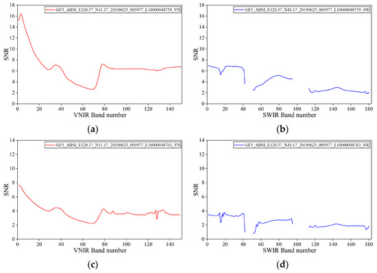
Figure 2.
SNRs of two AHSI data images. (a) SNR for GF5_AHSI_E120.37_N41.17_20190623_005977_L10000048759 at VNIR; (b) SNR for GF5_AHSI_E120.37_N41.17_20190623_005977_L10000048759 at SWIR; (c) SNR for GF5_AHSI_E120.53_N40.68_20190623_005977_L10000048763 at VNIR; (d) SNR for GF5_AHSI_E120.53_N40.68_20190623_005977_L10000048763 at SWIR.
3. Methods
Figure 3 shows the workflow of this study. This paper investigates the potential of high-frequency features (after DWT) in enhancing lithological classification accuracy in areas with vegetation cover. The method consists of five main components: (1) the pre-processing of rock spectra, vegetation spectra, and GF-5 AHSI data; (2) an analysis of the impact of vegetation on different rock spectra; (3) the one-dimensional DWT of simulated spectra and high-frequency feature extraction; (4) the selection of training sample types, optimal mother wavelet function, and decomposition level; and (5) the classification and accuracy assessment of AHSI image spectra.

Figure 3.
The method flowchart of this study.
3.1. Pre-Processing of Laboratory Spectra and GF-5 AHSI Data
3.1.1. Rock Reflectance Spectrum Measurement
Rock samples collected in the study area need to be measured for reflectance spectra and visually assigned names in the laboratory. The rock spectra were measured in the laboratory using an ASD FieldSpec 3 spectrometer (Malvern Panalytical Ltd., Boulder, CO, USA), covering the reflectance spectrum in the wavelength range of 350–2500 nm [40]. The sampling intervals were 1.4 nm for the 350–1000 nm range and 2 nm for the 1000–2500 nm range, with data output at a 1 nm interval across the entire wavelength range. During the measurement process, ten measurements were taken at different positions on the same rock sample, and the average value was used. To minimize measurement errors, the spectrometer was calibrated using a white reference board after each rock sample measurement.
3.1.2. Pre-Processing of GF-5 AHSI Data
The quality of the pre-processing of the AHSI data is a prerequisite for obtaining accurate image spectra. The pre-processing was carried out using the Pixel Information Expert-Hyp (PIE-Hyp) of PIESAT Information Technology Co., Ltd., Beijing, China [41].
After reading the raw data, the VNIR and SWIR data were combined. Due to wavelength overlap, the first four bands (wavelengths 1004.77–1030.05 nm) from the SWIR data were discarded. Bands in the range of 390.32–403.16 nm and 2471.11–2513.25 nm were removed due to too much striping and limited data readability. Two intervals in the SWIR bands (1350.58–1426.61 nm and 1797.02–1948.57 nm) were removed due to the effects of atmospheric water absorption. For the remaining bands, a global striping removal method was applied to eliminate vertical stripes in the image. Striping noise was removed column by column by first computing the ratio of global to local statistics along columns, then generating gain and bias, and finally applying a linear transformation to each pixel. Figure 4 shows a detailed view of the study area before and after striping removal. After applying the global striping removal method, the striping noise, smile effect, and bad lines in the image were improved. The next steps include radiometric calibration and atmospheric correction. Radiometric calibration converts the Digital Number (DN) values to apparent atmospheric reflectance, which is then converted to surface reflectance products after atmospheric correction. Atmospheric correction was performed using the 6S radiative transfer model. Finally, orthorectification was applied to correct spatial and geometric distortions, producing a multi-center projection orthophoto.
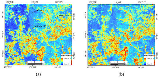
Figure 4.
Detailed view of GF-5 AHSI data (a) before pre-processing and (b) after pre-processing.
3.1.3. Pre-Processing of Reflectance Spectra
To investigate the lithological classification ability of the GF-5 AHSI data in vegetation–rock mixed areas, vegetation and rock spectra in the simulated data need to be consistent with the pre-processed AHSI data. The spectra of vegetation and rocks were convolved to match the spectral range of the pre-processed GF-5 AHSI data. The spectral range was from 407.44 nm to 2462.69 nm, with bands in the wavelength range of 1350.58–1426.61 nm and 1797.02–1948.57 nm removed. The process of convolving the spectra from the ASD to the AHSI data involves band removal and the spectral resampling of the remaining bands.
3.2. Mixed Simulation of Vegetation Spectra and Rock Spectra
For AHSI data in the study area, there is a mixture of rocks and vegetation in almost every pixel with a spatial resolution of 30 m. To study the influence of vegetation spectra on rock spectra and to verify whether the proposed method works under the condition of vegetation–rock mixing, mixed spectra need to be generated to simulate the mixing of different types of vegetation, varying vegetation abundances, and different types of rocks. In an ideal situation, the distribution of rock and vegetation within a mixed pixel is relatively independent, and the spectral reflectance energy is primarily added linearly [17]. A Linear Mixing Model (LMM) is used to simulate the mixed state of vegetation and rock spectra. The LMM is an effective modeling method when the mixing components are relatively independent in spatial distribution and the multiple scattering effect is ignored. This method has been widely used in areas where rocks and vegetation coexist and has good applicability in rocky desertification degree extraction and mountainous land cover mapping [42,43]. The rock endmembers are derived from resampled measured spectra, while the vegetation endmembers are sourced from the resampled USGS spectral library. It is assumed that the pixel reflectance is a linear combination of the rock and vegetation spectra, and the expression can be written as
where denotes the reflectance of a pixel, and and are the relative proportions of rock and vegetation within the pixel, respectively. and are the resampled rock and vegetation spectra, respectively.
In this study, linear spectral mixing models with vegetation fractions ranging from 0% to 60% (in 5% increments) were constructed to simulate the AHSI pixel spectra by combining vegetation and rock spectra.
3.3. DWT and High-Frequency Feature Extraction
How to effectively enhance the key information of rocks in the vegetation–rock mixing spectrum is crucial to improving the accuracy of rock classification. The high-frequency components of a spectrum reflect the rapid changes in reflectance with wavelength. High-frequency features at different decomposition levels can capture the changes in different scales in the spectral curve [44].
One-dimensional (1D) DWT decomposes the spectral curve into sub-signals across different frequency bands. Using scaling functions and wavelet functions, DWT extracts the low-frequency (approximation) and high-frequency (detail) components of the signal, respectively [45]. The further decomposition of the approximation coefficients from the first level yields coarser approximation coefficients (e.g., A2) and corresponding detail coefficients (e.g., D2).
In this study, six Daubechies (db) wavelet functions—Haar (db1), db2, db4, db6, db8, and db10—were used to perform one-, two-, and three-level DWT on the mixed spectral signals. The number following ‘db’ represents the number of vanishing moments (N); a higher N enables the better preservation of high-frequency sharp changes but also increases computational complexity. At each decomposition level i (i = 1, 2, 3), the spectral signal is processed using orthogonal filter banks through convolution and downsampling to obtain the low-frequency (approximation) coefficients Ai and the high-frequency (detail) coefficients Di (Figure 5). The scaling and wavelet functions of the mother wavelet used in this study are shown in Figure 6.
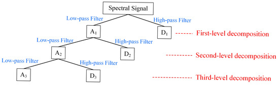
Figure 5.
One-dimensional discrete wavelet decomposition process of spectral signals.
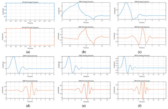
Figure 6.
Scaling functions and wavelet functions of (a) Haar, (b) db2, (c) db4, (d) db6, (e) db8, and (f) db10.
In the wavelength domain, the sampling frequency is analogous to the spatial frequency and can be expressed as follows:
Using the GF-5 AHSI data as an example, the sampling interval () of the VNIR band is 5 nm. According to the Nyquist–Shannon sampling theorem, the maximum resolvable frequency is [46]. The frequency range of the first-level high-frequency coefficients (D1) is , the second-level (D2) corresponds to , and the third-level (D3) corresponds to . Given that the product of wavelength and frequency is constant, higher-level decompositions capture larger-scale spectral variations, while lower-level high-frequency coefficients reflect finer-scale differences.
To extract multiscale high-frequency coefficients, the low-frequency approximation coefficients (Ai) were discarded, and all high-frequency detail coefficients (Di) were used to reconstruct the signal via Inverse Discrete Wavelet Transform (IDWT). The reconstructed signals replaced the original mixed spectral reflectance and were input into the classifier. By reconstructing all high-frequency components, subtle differences between mixed spectra were significantly enhanced, facilitating the subsequent discrimination of rock types. In this study, the format ‘mother wavelet_decomposition level’ was used to denote different sets of reconstructed high-frequency features. For example, the high-frequency features reconstructed from a level 2 decomposition using the db2 wavelet are denoted as db2_2. The extraction of high-frequency features was performed using the Wavelet Toolbox in MATLAB R2023a [47,48].
The SAM was used to evaluate the similarity between the simulated mixed pixel spectra and the original rock spectra (or high-frequency features of rocks). In the field of remote sensing land-use classification, a SAM of 0.1 is commonly used as a threshold [49]. When the SAM exceeds 0.1, the two spectral signatures may be considered to belong to different classes. The expression for the SAM is given by the following equation:
When DWT is not applied, x1 and x2 represent the vegetation–rock mixed spectrum and the rock spectrum of the same rock sample, respectively. When classification is performed using high-frequency features, x1 represents the high-frequency components (after normalization) of the mixed spectra, and x2 represents the rock spectrum.
The high-frequency features need to be normalized before calculating the SAM using the following equation:
where d denotes the high-frequency feature curve, and dmin and dmax represent the minimum and maximum values of the high-frequency features, respectively.
3.4. Classification of Simulated Mixed Spectra
3.4.1. Types of Training Samples
In geological surveys, latitude and longitude, rock type, and field or laboratory spectra are usually obtained for sample points. In previous studies on lithological classification using hyperspectral data, both image spectra and laboratory-measured rock spectra were used as training samples for classification. In areas with well-exposed rocks, good classification results were achieved using the image spectra of rock units as training samples [11,50]. However, in areas covered by vegetation, it is challenging to obtain pure rock spectra from image pixels. One approach is to use the laboratory spectra as training samples, and the other is to use the image spectra of the examined image pixels as training samples. In this study, simulated vegetation–rock mixed spectra are employed to evaluate the classification performance of these two training sample selection strategies and to assess the impact of high-frequency features on classification accuracy.
3.4.2. Bayesian-Optimized Random Forest Classifier
To investigate the effectiveness of high-frequency spectral components in enhancing lithological discrimination, a stable and efficient classifier is essential to ensure the reliability of comparative experiments. The RF classifier has been widely used in lithological mapping based on remote sensing data and has an advantage when dealing with high-dimensional data [51]. RF builds an ensemble of decision trees and aggregates their predictions via a majority voting mechanism to achieve high classification accuracy. At each node split in a decision tree, only some features (rather than all of them) are randomly selected as candidate splitting variables, which effectively mitigates the risk of overfitting when dealing with high-dimensional data.
The RF classifier involves two key parameters: the number of features selected at each node split (mtry) and the total number of decision trees (ntree). Increasing the ntree generally improves the stability of predictions but at the cost of a higher computational time. In this study, the ntree was set to 1000, which is a commonly used and empirically stable value that maintains acceptable computational efficiency [52]. A large mtry value may lead to a higher correlation between trees and potential overfitting, while a small mtry value may weaken the learning capacity of individual trees, resulting in underfitting.
For high-dimensional data such as spectral data, Bayesian optimization is particularly suitable for dynamically tuning discrete hyperparameters such as mtry during the model training process. The Bayesian-optimized RF classification process and accuracy assessment were implemented using the randomForest [53], rBayesianOptimization [54], and caret packages [55] in R version 4.2.3.
The Bayesian optimization process for selecting the optimal mtry value included the following steps:
- Data Partitioning: The dataset was split into 70% training and 30% testing subsets while maintaining a balanced class distribution.
- Hyperparameter Optimization: The search space for mtry was defined as integers from 1 to 30, with ntree fixed at 1000. Five-fold cross-validation on the training set was used to evaluate model performance, and the average overall accuracy was set as the optimization objective. After 10 random initializations, 20 iterations of Bayesian optimization were performed using the Expected Improvement (EI) acquisition function.
- Model Training: The optimal mtry value determined by the Bayesian optimization was used to train the final RF model on the entire training set.
- Accuracy Assessment: The model was evaluated on the test set using the overall accuracy (OA), Kappa coefficient (KAPPA), Precision, Recall, and F1-score. These indicators are calculated using the following equation:
3.5. Classification of Image Spectra
3.5.1. Estimation of Fractional Vegetation Cover
The effectiveness of high-frequency components in extracting subtle lithological information is influenced by the level of vegetation coverage. Following the analysis of simulated data, representative pixels in the study area were selected for validation.
A pixel binary model was employed to estimate the Fractional Vegetation Cover (FVC) across the study area. This model assumes that each pixel is composed of a vegetated and a non-vegetated portion [56,57]. The FVC is calculated using the following expression [58]:
where NDVI is the Normalized Difference Vegetation Index of the target pixel. NIR is the reflectance derived from the pixel value at 860 nm, and R is obtained from the pixel value at 651 nm in the GF-5 AHSI data. NDVImin corresponds to the NDVI of pure non-vegetation (rock) pixels, while NDVImax represents the NDVI of pure vegetation pixels. Under ideal conditions, NDVImin approaches zero, and NDVImax approaches one. To mitigate the influence of outliers, water bodies were masked before NDVI extraction. In this study, NDVImin was defined as the 0.5th percentile, and NDVImax as the 99.5th percentile of the NDVI cumulative distribution within the study area.
3.5.2. Lithological Classification Based on Image Spectra
Sample image pixels with FVC values of less than 0.6 were retained. The image spectra of filtered samples were extracted and used for lithological classification based on their high-frequency features derived from DWT. The mother wavelet function, decomposition level, and type of training samples used for DWT were selected based on the optimal parameters identified in the spectral mixing simulations. A Bayesian-optimized Random Forest classifier was also employed for classification. To ensure robust and stable classification performance, five-fold cross-validation was conducted after determining the optimal mtry value. Classification accuracy was evaluated using the OA, KAPPA, Recall, Precision, and F1-score. For each rock class, the available samples were randomly divided into five folds, with four folds used for training and the remaining one for testing in each iteration. The final performance metrics were reported as the average results across the five-fold cross-validation [59].
4. Results
4.1. Rock Spectra, Vegetation Spectra, and Simulated Mixed Spectra
4.1.1. Rock Spectral Features
Based on the wavelength range of the preprocessed AHSI data, the averaged rock reflectance spectra measured by the ASD spectrometer and their convolved counterparts are shown in Figure 7. Due to the vibrational absorption of water molecules, the rock spectra form absorption features near 1.40 μm and 1.90 μm. These absorption features are key indicators for distinguishing rock types in measured spectra. However, due to atmospheric water vapor absorption, such features are not retrievable in GF-5 AHSI data.
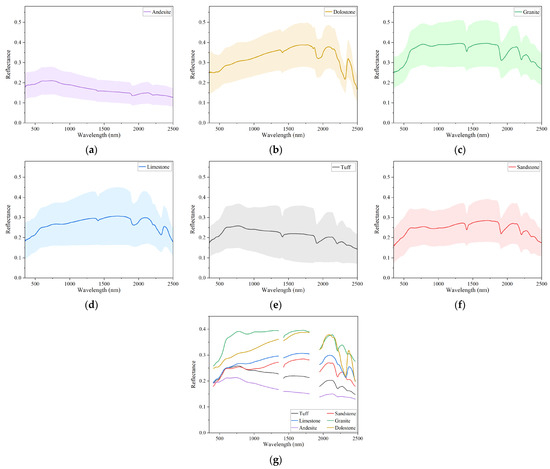
Figure 7.
(a–f) Average rock spectra measured using the ASD spectrometer (shaded regions around the curves represent the standard deviation across samples); (g) spectral curves of rocks convolved to the GF-5 AHSI sensor.
Within the spectral range of 0.41–1.80 μm, granite, dolomite, and limestone exhibit increasing reflectance, while andesite and tuff display decreasing reflectance. Granite and sandstone both show iron-related absorption features near 0.90 μm. An absorption peak at 2.20 μm in granite spectra may be attributed to clay alteration. Dolomite presents an absorption feature at 2.31 μm, resulting from carbonate vibrations. Limestone exhibits an absorption feature at 2.32 μm and a weaker feature at 2.21 μm. Sandstone, andesite, and tuff have absorption features near 2.21 μm. Overall, granite and dolomite display higher reflectance values, whereas andesite and tuff show relatively lower reflectance.
4.1.2. Vegetation Spectral Features
Green vegetation contains pigments, such as chlorophyll, lutein, and anthocyanins, as well as biochemical components like carbon and nitrogen, which produce absorption features at different wavelengths in the reflectance spectrum. The spectrum of green grass exhibits a gradual increase in reflectance between 0.41 and 0.55 μm, with a reflectance peak at 0.55 μm. A rapid increase occurs between 0.68 and 0.85 μm, culminating in a reflectance maximum near 0.85 μm. Distinct absorption features are observed around 0.68 μm, 0.98 μm, 1.20 μm, and 1.45 μm. The increase in the proportion of the cellulose and lignin content of golden grass changed the scattering characteristics of the tissue, and there were significant absorption valleys in the SWIR band. Golden grass shows a gradual reflectance increase from 0.41 to 1.32 μm, with absorption features near 1.45 μm, 1.72 μm, and 2.10 μm and reflectance peaks at 1.65 μm, 2.00 μm, and 2.22 μm. Bush exhibits a similar spectral trend to green grass but generally shows lower reflectance. The bush spectrum has absorption features at 0.67 μm, 0.98 μm, and 1.20 μm, along with reflectance peaks at 0.92 μm, 1.10 μm, 1.28 μm, and 1.63 μm. Influenced by compounds such as lichen acids, polysaccharides, and phenols, lichens exhibit multiple absorption features in the SWIR band. Lichen shows a rapid increase in reflectance between 0.41 and 0.57 μm, followed by a decrease from 0.57 to 0.68 μm, and then a gradual increase from 0.68 to 1.35 μm (with a steeper slope from 0.68 to 0.74 μm and a gentler slope from 0.74 to 1.35 μm). The lichen spectrum presents absorption features around 0.68 μm, 1.46 μm, and 2.09 μm, with reflectance peaks near 0.57 μm, 1.65 μm, 2.01 μm, and 2.22 μm (Figure 8).
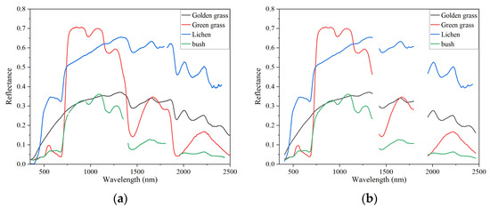
Figure 8.
(a) Vegetation spectra collected from USGS spectral library version 7; (b) spectral curves of vegetation convolved to the GF-5 AHSI sensor.
4.1.3. Simulated Mixed Spectral Features
The vegetation impact on the rock spectra depends on the reflectance intensity and absorption depth. Figure 9 shows the linear mixing results between different vegetation types and rock spectra.
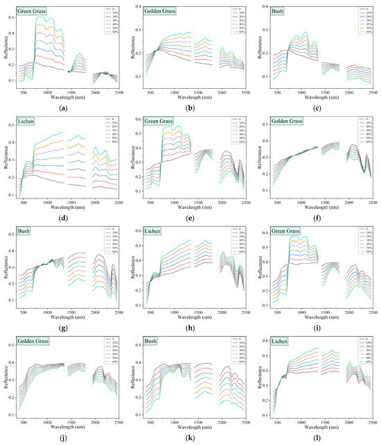
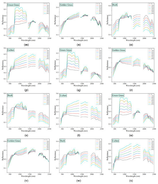
Figure 9.
Simulated mixed spectra of different rocks with varying vegetation contents: (a–d) andesite, (e–h) dolomite, (i–l) granite, (m–p) limestone, (q–t) tuff, and (u–x) sandstone.
Andesite exhibits a relatively flat reflectance curve without distinctive absorption or reflection peaks, and even a 10% vegetation fraction can cause the mixed spectrum to show similar features to the vegetation spectrum. The 2.31 μm absorption feature of dolomite is less affected by vegetation, while its relatively smooth spectral curve between 0.50 and 1.8 μm begins to show multiple reflection peaks under the influence of green grass and bushes. The granite spectrum is most affected by lichen; when the lichen coverage exceeds 30%, the reflection peak at 2.13 μm disappears, which consequently weakens the absorption feature at 2.20 μm. The 2.32 μm absorption feature of limestone is stable under vegetation influence. In the 0.41–1.8 μm range, limestone reflectance is sensitive to green grass, and between 0.76 and 1.35 μm, it is sensitive to bushes. The reflection peak at 2.10 μm for limestone disappears when golden grass coverage exceeds 20%. The absorption depth at 2.21 μm for tuff gradually decreases as the vegetation content increases and disappears when lichen coverage exceeds 40%. In the 0.41–1.35 μm range, the slope of the sandstone spectrum is significantly influenced by green grass and bushes. The depth of the absorption feature near 2.21 μm also decreases with increasing vegetation and disappears when lichen exceeds 50%.
Figure 10 shows the SAM between the mixed spectra containing different contents of vegetation and the vegetation spectra. In general, the SAM decreases as the vegetation content increases. When the green grass content was above or close to 60%, the value of the SAM was lower than 0.2. The smaller SAM between the mixed spectrum containing golden grass and lichen and the vegetation spectrum indicates that the similarity between the mixed spectrum and the vegetation spectrum is high.
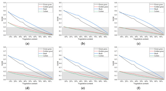
Figure 10.
SAM between the mixed spectra containing different contents of vegetation and the vegetation spectra. The rock types in the mixed spectrum are (a) andesite, (b) dolostone, (c) granite, (d) limestone, (e) tuff, and (f) sandstone.
Figure 11 illustrates the impact of different vegetation cover levels on the reflectance ratio of rocks. The reflectance ratio directly reflects the presence of spectral absorption features or reflectance peaks. When the ratio approaches 1, it indicates that the corresponding absorption or reflection feature is nearly eliminated. When the ratio crosses 1, it suggests that the original spectral feature of the rock has disappeared, reducing the distinctiveness of the rock type. Taking dolomite as an example, the B2083nm/B2032nm reflectance ratio decreases with the increasing coverage of lichen, golden grass, and bushes but increases with increasing green grass coverage. As part of the reflectance peak near 2.09 μm, the B2083nm/B2032nm ratio is greater than 1; however, when the coverage of golden grass or lichen exceeds 20%, the ratio drops below 1. This change indicates that the corresponding spectral feature is masked, thereby weakening the recognizable features of the rock.
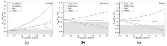
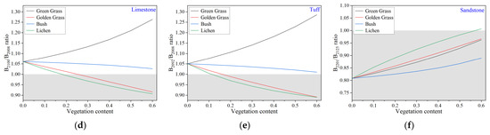
Figure 11.
Specific band ratios in different vegetation–rock mixed spectra. The rock types in the mixed spectrum are (a) andesite, (b) dolostone, (c) granite, (d) limestone, (e) tuff, and (f) sandstone.
4.2. High-Frequency Feature Extraction Using DWT
4.2.1. High-Frequency Wavelet Features of Rocks
After applying DWT to the reflectance spectra, the high-frequency (detail) features correspond to regions with rapid spectral variations. These high-frequency components capture the local details of the spectral curves, such as rapid changes in absorption troughs. In relatively flat regions of the spectra, the absolute values of the high-frequency coefficients tend to be small. Rocks have distinct absorption features within the 1.95–2.46 μm range, and the regions of higher energy in the high-frequency domain typically correspond to prominent absorption features in the spectra. Figure 12 presents a comparison between the average rock spectra and their high-frequency components (after db8_2). The steep edges and rapid variations around the absorption troughs in the dolomite spectrum are reflected as large high-frequency coefficients in the discrete wavelet decomposition.
Figure 12.
Convolved rock spectra and corresponding high-frequency features extracted by DWT (after db8_2): (a) andesite, (b) dolomite, (c) granite, (d) limestone, (e) tuff, and (f) sandstone.
4.2.2. High-Frequency Wavelet Features of Simulated Mixed Spectra
Figure 13 shows the mixed spectra and corresponding high-frequency coefficients (db8_2) at 20% green grass content. Under the influence of the green grass spectrum, the simulated mixed spectra and their high-frequency features of various rocks exhibit strong similarity in the 0.41–1.35 μm range. In the 1.95–2.46 μm range, the high-frequency coefficients of dolomite have the highest amplitude, and those of andesite have the smallest amplitude. These high-frequency features remain effective in enhancing the spectral differences among rocks even with a small amount of green grass.
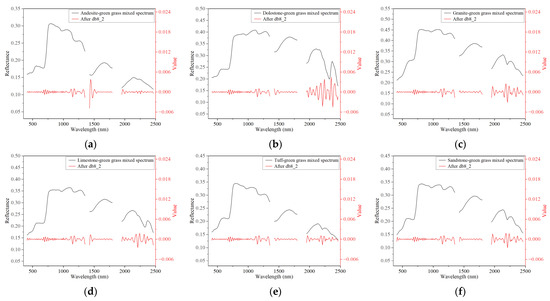
Figure 13.
Simulated vegetation–rock mixed spectra and corresponding high-frequency features (after db8_2) at 20% green grass coverage: (a) andesite, (b) dolomite, (c) granite, (d) limestone, (e) tuff, and (f) sandstone.
Figure 14 presents the mixed spectra and corresponding high-frequency coefficients (db8_2) under 40% bush coverage. Similarly to the case with green grass, the simulated mixed spectra and high-frequency features are highly consistent across different rock types in the 0.41–1.35 μm range. However, compared to the green grass spectrum, the bush spectrum is relatively flatter in the 1.95–2.46 μm range. Except for andesite, the other rock spectra partially retain their absorption features in the 1.95–2.46 μm range.
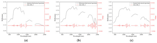
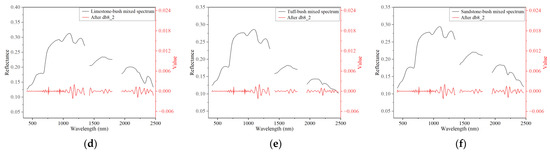
Figure 14.
Simulated vegetation–rock mixed spectra and corresponding high-frequency features (after db8_2) at 20% bush coverage: (a) andesite, (b) dolomite, (c) granite, (d) limestone, (e) tuff, and (f) sandstone.
4.3. Impact of Vegetation on Rock Classification
The SAM between the simulated mixed spectra and the original rock spectra reflects the influence of vegetation on rock spectral features. For rock spectra, when green grass coverage exceeds 10%, bush or lichen coverage exceeds 15%, or golden grass coverage exceeds 25%, the SAM between the mixed and rock spectra exceeds 0.1. When the differences between the mixed spectra and the original rock spectra are pronounced, differentiating between rock types becomes challenging. Figure 15a shows the SAM between the simulated mixed spectra and the rock spectra, while Figure 15b–d display the SAM between the high-frequency features extracted from the simulated mixed spectra and those from the rock spectra. When green grass, golden grass, and bush coverage are below 60% and lichen coverage is below 40%, the SAM between the high-frequency features remains below 0.1. This indicates that the high-frequency coefficients after DWT are less susceptible to vegetation interference than the original reflectance, potentially providing an advantage in distinguishing rock types.
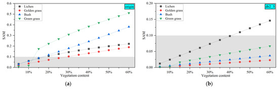
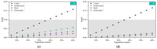
Figure 15.
SAM between the mixed spectra and the original rock reflectance (or rock high-frequency features) under various vegetation cover levels, derived from the following: (a) mixed spectral reflectance; (b) high-frequency features (db2_3); (c) high-frequency features (db6_3); and (d) high-frequency features (db8_2).
4.4. Classification Accuracy Assessment of Simulated Mixed Spectra
The spectra involved in the classification are the result of mixing the reflectance spectra of the rocks in the study area with the reflectance spectra of the vegetation in the USGS spectral library. All rock spectra formed with vegetation of a certain weight are considered as one dataset. The properties of each mixed spectral curve are consistent with the properties of the rocks involved in spectral mixing. Each dataset has the same number of spectral curves, and the accuracy assessment is performed independently in each dataset.
4.4.1. Using Simulated Mixed Spectra as Training Samples
The purpose of using simulated mixed spectra as training samples is to emulate the classification performance achieved when using image spectra as training data. Without DWT, the OAs of db8_1, db8_2, and db8_3 are shown in Figure 16, while classification results using other mother wavelet functions and decomposition levels are presented in Table A2, Table A3, Table A4 and Table A5 in Appendix A. Table A6 shows the Bayesian optimization process based on db8_2 features at 20% vegetation content (using simulated mixed spectra as training samples).
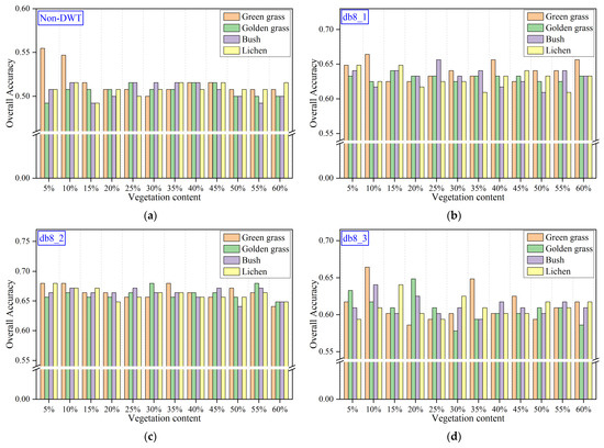
Figure 16.
OA for simulated vegetation–rock mixed spectra (with simulated mixed spectra as training samples): (a) non-DWT; (b) db8_1; (c) db8_2; (d) db8_3.
Without DWT, the OA of the simulated mixed spectra ranges between 0.49 and 0.55. The overall accuracy of green grass–rock mixed spectra is markedly reduced when vegetation content exceeds 10%. This may be attributed to green grass coverage exceeding 10%, which obscures the characteristic bands of the rock. Classification accuracy declines when the inter-class separability among training samples decreases. The OA for db8_1 is between 0.61 and 0.66, for db8_2, it is between 0.64 and 0.68, and for db8_3, it is between 0.58 and 0.66. Regardless of the mother wavelet function and the number of decomposition levels used in the DWT, the OA increased by more than 10% after classification using the high-frequency component. Compared to other types of high-frequency features, the high-frequency components extracted using the db8 wavelet yield higher overall classification accuracy. As illustrated by the bar charts, the OA of db8_2 exhibits minimal fluctuation with increasing vegetation cover, maintaining high values.
The F1-score provides insights into the changes in OA. Figure 17 shows the F1-scores obtained when classifying based on the reflectance of simulated mixed spectra. Granite has the highest F1-score (around 0.70), followed by limestone (around 0.55), while andesite shows the lowest F1-score (around 0.30). F1-scores for dolomite, sandstone, and tuff fluctuate around 0.45. In classifications using simulated mixed spectra as training samples, F1-scores generally remain stable regardless of the proportions of golden grass, bush, or lichen. For grass–rock mixed spectra, in the 5–15% green grass content range, the F1-score of sandstone decreases from 0.57 to 0.45, while the F1-scores of limestone and andesite first increase and then decrease. When the green grass content exceeds 15%, the F1-scores stabilize.
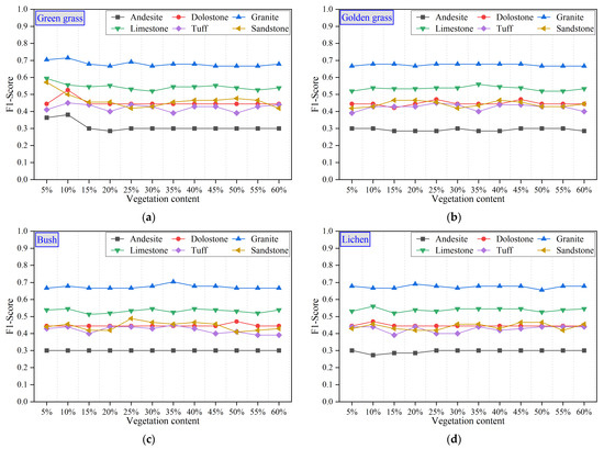
Figure 17.
F1-scores based on the classification of simulated mixed spectral reflectance (using simulated mixed spectra as training samples). The vegetation types in the mixed spectrum are (a) green grass, (b) golden grass, (c) bush and (d) lichen.
Considering both the F1-score and OA, the high-frequency components extracted using db8_2 yielded the best classification performance. Figure 18 illustrates the F1-scores obtained from classification based on the high-frequency features (db8_2) of simulated mixed spectra (with simulated mixed spectra used as training samples). Across all four types of mixed spectra, andesite showed the lowest F1-score (approximately 0.3), while granite and limestone exhibited the highest F1-scores (approximately 0.7 and 0.55, respectively). After applying high-frequency components, the F1-score of granite increased from 0.70 to 0.80, and that of limestone from 0.55 to around 0.75. The F1-scores of dolomite, sandstone, and tuff also improved from approximately 0.45 to about 0.60, 0.68, and 0.55, respectively. Only the classification performance of andesite declined after using high-frequency components. In Figure 18c, the classification accuracy of all rocks decreases when the bush content increases from 45% to 50%. However, for the remaining vegetation content, the F1-scores fluctuated with increasing vegetation content but did not exhibit a clear increasing or decreasing trend.
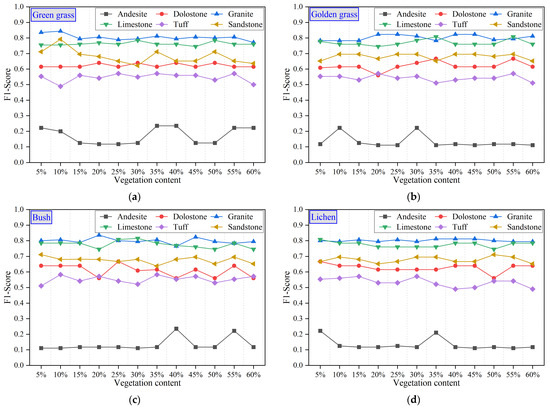
Figure 18.
F1-scores from classification using the high-frequency features (db8_2) of simulated mixed spectra (using simulated mixed spectra as training samples). The vegetation types in the mixed spectrum are (a) green grass, (b) golden grass, (c) bush and (d) lichen.
4.4.2. Using Original Rock Spectra as Training Samples
The purpose of using original rock spectra as training samples is to simulate classification performance based on laboratory spectra. When classifying with original reflectance, the OA ranges from 0.20 to 0.53. The OA decreased with increasing green grass, golden grass, and bush content. For lichen, the OA decreases with increasing coverage when the lichen content is below 50% but increases from 0.27 to 0.34 when the lichen coverage exceeds 50%.
The high-frequency features extracted by db8_2 yield the best classification performance. The OA generally decreases with increasing golden grass, bush, and lichen content. When the green grass content is below 30%, the OA also decreases; however, when it exceeds 30%, the OA begins to increase with higher green grass coverage. When vegetation coverage exceeds 40%, rock classification accuracy is significantly affected. In both bush–rock and lichen–rock mixtures, the OA drops below 0.5, indicating increased difficulty in classification (Figure 19).
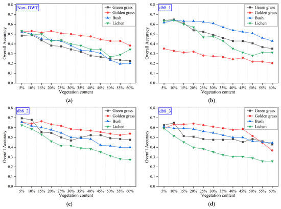
Figure 19.
OA for simulated vegetation–rock mixed spectra (with original rock spectra as training samples): (a) non-DWT, (b) db8_1, (c) db8_2, and (d) db8_3.
Figure 20 illustrates the F1-scores of different rock types after classification using mixed spectral reflectance and reveals the reason for the decrease in the F1-scores with increasing vegetation content. For green grass–rock mixtures, the F1-score of granite decreases with increasing green grass content (from 0.68 to 0.33). The F1-score of tuff fluctuates around 0.3. The F1-scores for andesite, dolomite, limestone, and sandstone drop to zero when the green grass proportion reaches 20%, 40%, 30%, and 35%, respectively. In contrast, golden grass has a lesser impact on classification performance. For golden grass–rock mixtures, the F1-scores of granite, sandstone, and limestone fluctuate around 0.7, 0.45, and 0.45, respectively. The F1-score of dolomite increases from 0.44 to 0.74 before decreasing to 0.32, and andesite drops to zero when the golden grass content exceeds 45%. For bush–rock mixtures, the F1-score of tuff fluctuates around 0.35, while the scores of other rock types decrease with increasing bush content. For the classification results of lichen–rock mixing spectra, the F1-scores of granite and andesite decrease as lichen coverage increases, and the F1-scores of tuff, limestone, dolomite, and sandstone fluctuate greatly with the change in lichen content.
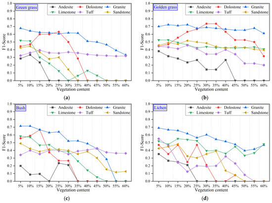
Figure 20.
F1-scores based on the classification of simulated mixed spectral reflectance (using original rock spectra as training samples). The vegetation types in the mixed spectrum are (a) green grass, (b) golden grass, (c) bush and (d) lichen.
Figure 21 presents the F1-scores derived from classifications based on the high-frequency components (db8_2) of the mixed spectra, using original rock spectra as training samples. For grass–rock mixtures, the F1-scores of limestone and granite decreased from 0.82 and 0.83 to 0.66 and 0.63, respectively, with increasing grass coverage. The F1-scores of dolomite and sandstone dropped to zero at 35% grass content, while the F1-score of andesite increased when grass coverage exceeded 30%. For golden grass–rock mixtures, andesite showed the lowest F1-score (~0.1), and both dolomite and sandstone exhibited significant drops in F1-scores when the golden grass coverage exceeded 15%. In bush–rock mixtures, andesite samples were not correctly classified, and the F1-scores of dolomite and sandstone sharply declined beyond 15% bush content. For lichen–rock mixtures, the F1-scores of all rock types decreased when the lichen coverage exceeded 15%; andesite, tuff, and limestone were not correctly classified.
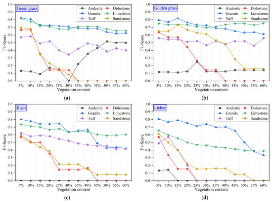
Figure 21.
F1-scores based on classification using the high-frequency features (db8_2) of simulated mixed spectra (using original rock spectra as training samples). The vegetation types in the mixed spectrum are (a) green grass, (b) golden grass, (c) bush and (d) lichen.
4.5. Evaluation of Classification Accuracy Using AHSI Image Spectra
4.5.1. Selection of Rock Samples
Based on the results from the simulated mixed spectra, and considering the OA, F1-score, and SAM, the high-frequency feature (db8_2) has excellent performance in the identification of dolomite, granite, limestone, sandstone, and tuff within vegetation–rock mixed areas where the FVC is below 60%. To further evaluate the effectiveness of high-frequency features in such mixed conditions, rock classification was conducted using hyperspectral imagery from GF-5 AHSI data.
Rock samples were selected based on FVC values, retaining only those with an FVC < 0.6. A total of 226 sample points met this criterion, including 46 tuff, 44 sandstone, 44 limestone, 68 granite, and 24 dolomite samples. Figure 22a shows the frequency distribution of these samples, with most FVC values falling within the 0.2–0.4 and 0.5–0.6 intervals. Figure 22b illustrates the image spectra of granite samples with FVC values of 0.51 and 0.08. As the FVC increases, the absorption depth at 0.67 μm, 1.48 μm, and 2.04 μm becomes more pronounced.
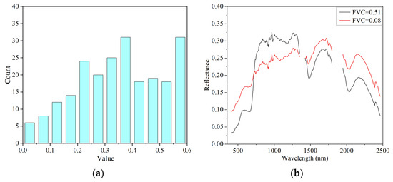
Figure 22.
(a) Frequency of samples with FVC < 0.6; (b) image spectra of granite samples with FVC values of 0.51 and 0.08.
4.5.2. Classification Accuracy Assessment Using Image Spectra
Image spectra have been shown in simulation experiments to be potentially more suitable for rock classification in vegetation-influenced areas. Table 4 and Table 5 present the average Precision, Recall, F1-score, OA, and KAPPA of five rock types under five-fold cross-validation, comparing results with and without the use of DWT. After applying high-frequency components (db8_2), the OA increased from 0.37 to 0.53, and the KAPPA improved from 0.18 to 0.38. The F1-score of tuff increased by 0.48, granite by 0.11, and sandstone by 0.13. The classifier showed high precision in predicting tuff, with 91% of samples labeled as tuff being correct; however, due to a high miss-detection rate, its F1-score was 0.71. Dolomite was the only rock type for which the accuracy decreased after applying high-frequency features, possibly due to the limited number of samples.
Table 4.
Classification accuracy using image spectral reflectance.
Table 5.
Classification accuracy using high-frequency features (db8_2) of image spectra.
5. Discussion
As is well known, vegetation cover in humid and semi-humid regions presents significant challenges for lithological mapping and geological surveys using remote sensing. Except where vegetation entirely obscures rocks, this study focuses on mixed pixels in rock outcrop areas with vegetation interference and proposes the use of high-frequency features derived from DWT to improve lithological classification accuracy.
In the 0.41–1.80 μm wavelength range, rock spectra are significantly affected by green vegetation. When the vegetation cover exceeds 20%, the spectral curves show a trend of similarity with the green vegetation spectra, and the rock features are masked. The simulated spectrum of andesite shows no distinct absorption features from 1.95 μm to 2.46 μm. Guo et al. [30] noted that rock spectra may have large intra-class variability, increasing the likelihood of spectral confusion among rock types. The absorption features near 2.3 μm in dolomite and limestone are less affected by golden grass. Other rock spectra are more affected by golden grass due to their shallow absorption features between 2.1 and 2.3 μm. In vegetated areas, analyzing the seasonal variation of overlying vegetation can improve the identification of underlying rocks. Linear spectral mixing models with varying vegetation cover reveal not only the progressive masking of rock spectra but also the spectral sensitivity of different rocks to vegetation. For a given rock type, classification accuracy generally decreases with increasing vegetation cover, though the trend is not strictly linear. At similar vegetation levels, differences in rock spectral sensitivity to vegetation may aid in distinguishing rock types.
Multiscale features derived from wavelet decomposition are commonly used for surface parameter retrieval, such as elemental inversion [60]. However, high-frequency features are rarely employed independently for feature enhancement. Due to significant intra-class variability, rock spectra often have similar trends but differ in intensity. This may explain why using only high-frequency features can still improve classification accuracy.
Reconstruction using only first-level high-frequency coefficients captures the highest frequency details in the spectrum. Second-level coefficients represent lower frequencies than the first level but remain higher than the corresponding low-frequency part. When combining high-frequency coefficients from the first two (or three) levels, the reconstructed signal includes multiscale frequency details, covering both fine and moderate spectral variations. Figure 23 shows the sandstone reflectance and corresponding multiscale high-frequency features in the 1.95–2.46 μm range. As more high-frequency levels are included, the reconstructed values increase. The reconstruction from first-level coefficients alone fluctuates around zero with the smallest magnitude. Although first-level high-frequency components are often treated as noise, Guo et al. [30] confirmed their relevance in rock classification, and thus, we retained them. A higher number of vanishing moments leads to smoother reconstructed features, which benefits the extraction of slowly varying spectral details. In contrast, small vanishing moments are effective in capturing short, high-frequency features and may produce jagged fluctuations in regions with abrupt spectral changes.
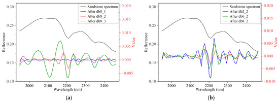
Figure 23.
(a) Sandstone reflectance and high-frequency features reconstructed at different scales; (b) sandstone reflectance and high-frequency features reconstructed using different mother wavelets. Reflectance is plotted on the left y-axis, and high-frequency features are plotted on the right y-axis.
Ahmad et al. [61] explored the capability of AVIRIS and ASTER data in extracting anorthosite and metagabbro in areas with vegetation cover using the LMM and Hapke model. The LMM and Hapke model have their own strengths in rock abundance extraction but hyperspectral imagery performs better in rock abundance mapping. Their study provides a good method for extracting a single type of rock or a few types of rocks in vegetated areas. Our study attempted to distinguish a number of rock types in areas with moderate or low vegetation cover, and the accuracy of lithology identification needs to be further improved, limited by the fact that some of the rock spectra have low reflectance and lack absorption features. Using vegetation spectra from the USGS spectral library to participate in the simulation allowed us to highlight the absorption characteristics of typical vegetation spectra, but in future work, we are considering collecting vegetation spectra during field surveys to reduce the difference between simulated and real classifications. At a higher vegetation cover, multiple scattering from vegetation may cause nonlinear spectral responses and mask rock absorption features. For these purposes, nonlinear mixture models such as the Hapke model are also necessary to be included in future simulations.
In classifications using only high-frequency components, the shape of the spectral curve is emphasized, while absolute reflectance values are ignored. To maintain a stable number of features and avoid errors from varying feature selection methods, original reflectance and low-frequency DWT components were not included. If more features are included, dimensionality reduction and feature selection become necessary steps. In vegetation–rock mixed areas, classification using only high-frequency components outperforms reflectance-based results, suggesting that spectral trends and shapes are more important. This study focused on mixed pixels with a vegetation cover below 60%. The main reason for this is that widely distributed green vegetation dominates the mixed spectrum by the vegetation spectrum at levels above 60%. In densely vegetated areas, hyperspectral geological mapping relies on plant–soil relationships. Rock types can be identified and classified by analyzing subtle differences in the spectra of vegetation growing around the rock. Identifying vegetation band wavelengths that reflect underlying rock properties could further enhance the role of hyperspectral data in lithological mapping.
6. Conclusions
The aim of this study is to enhance rock spectral features in sparse vegetation–rock mixed spectra, thereby improving rock classification accuracy using GF-5 hyperspectral data. The results show that, regardless of vegetation type (green grass, golden grass, bushes, or lichens), high-frequency features derived from DWT effectively exclude vegetation interference and highlight rock characteristics. By simulating mixed spectra with varying vegetation and rock proportions, the influence of different vegetation spectra on rock signatures was analyzed. Optimal parameters—mother wavelet db8 and decomposition level 2—were selected based on their classification performance across simulated spectra. When using rock reflectance or rock high-frequency features as training data, high-frequency features improved the average OA by 0.12 (from 0.39 to 0.51). Using simulated mixed spectra as training data, the OA increased by 0.15 (from 0.51 to 0.66). In validation with AHSI image spectra, the classification accuracy of granite, limestone, and tuff improved with high-frequency features. More vegetation information, such as the height and cover of vegetation at each sample point, will need to be recorded during future field surveys. For areas with higher vegetation cover, further improvements may rely on identifying relationships between the vegetation and underlying rocks or incorporating auxiliary data such as the DEM to support lithological mapping in humid and semi-humid regions.
Author Contributions
Conceptualization, S.G. and Q.J.; methodology, S.G.; software, S.G.; validation, S.G. and Q.J.; formal analysis, S.G.; investigation, S.G.; resources, Q.J.; data curation, S.G.; writing—original draft preparation, S.G.; writing—review and editing, S.G.; visualization, S.G.; supervision, Q.J.; project administration, Q.J.; funding acquisition, Q.J. All authors have read and agreed to the published version of the manuscript.
Funding
This research was funded by the China Geological Survey Project, grant number DD20191011.
Data Availability Statement
The field survey data presented in this article are not readily available because the data are part of an ongoing study. GF-5 AHSI data can be accessed through the website: https://data.cresda.cn/#/2dMap (accessed on 15 December 2024) and the copyright owner of the data is China Centre for Resources Satellite Data and Application. The precipitation dataset is provided by National Tibetan Plateau/Third Pole Environment Data Center (http://data.tpdc.ac.cn (accessed on 5 December 2024)). The vegetation dataset is provided by National Cryosphere Desert Data Center. (http://www.ncdc.ac.cn (accessed on 1 December 2024)).
Acknowledgments
The authors would like to thank the students and teachers of Jilin University who provided assistance during the field work.
Conflicts of Interest
The authors declare no conflicts of interest.
Abbreviations
The following abbreviations are used in this manuscript:
| PRISMA | Prototype Research Instruments and Space Mission Technology Advancement |
| AHSI | Advanced Hyperspectral Imager |
| AVIRIS | Airborne Visible Infrared Imaging Spectrometer |
| VNIR | visible to near-infrared |
| SWIR | shortwave infrared |
| SAM | spectral angle mapper |
| RF | Random Forest |
| SVMs | Support Vector Machines |
| CNNs | Convolutional Neural Networks |
| GF-5 | Gaofen-5 |
| PCA | Principal Component Analysis |
| MNF | Minimum Noise Fraction |
| NDVI | Normalized Difference Vegetation Index |
| DEM | Digital Elevation Model |
| LiDAR | Light Detection and Ranging |
| ATM | Airborne Thematic Mapper |
| SAVI | Soil-Adjusted Vegetation Index |
| DWT | Discrete Wavelet Transform |
| ASTER | Advanced Spaceborne Thermal Emission and Reflection Radiometer |
| GDEM | Global Digital Elevation Model |
| ASD | Analytical Spectral Devices |
| LMM | Linear Mixing Model |
| DN | Digital Number |
| db | Daubechies |
| IDWT | Inverse Discrete Wavelet Transform |
| EI | Expected Improvement |
| KAPPA | Kappa coefficient |
| OA | overall accuracy |
| FVC | Fractional Vegetation Cover |
| SNR | signal-to-noise ratio |
Appendix A
Table A1.
Geological units and codes in the study area.
Table A1.
Geological units and codes in the study area.
| Stratigraphic Age | Code | Geological Unit | Code | Geological Unit |
|---|---|---|---|---|
| Quaternary | Q | Sandy–silty clay and gravel layer | ||
| Cretaceous | k1y | Yixian formation: andesite, conglomerate, and tuff | ||
| Jurassic | J2tc | Tuchengzi formation: andesitic sandstone and tuffaceous sandstone | J2t | Tiaojishan formation: basalt, andesite, and tuffaceous sandstone |
| J1y | Yangcaogou formation: conglomerate and feldspathic sandstone | J1b | Beipiao formation: tuffaceous shale interbedded with coal seams | |
| J1x | Xinglonggou formation: basalt and andesite interbedded with volcanic breccia. | |||
| Triassic | T1h | Hongli formation: purple medium-coarse sandstone and tuffaceous sandstone | ||
| Permian | P1–2s | Shanxi formation: feldspathic sandstone interbedded with bauxitic shale | ||
| Carboniferous | C2-P1t | Taiyuan formation: coarse-grained feldspathic sandstone and bauxitic shale | ||
| Ordovician | O2m | Majiagou formation: limestone and dolomitic limestone | O1γ | Yeli formation: dolomitic limestone and bamboo leaf-shaped limestone |
| Cambrian | Ꞓ3c | Chaomidian formation: oolitic limestone interbedded with bamboo leaf-shaped limestone | Ꞓ2z | Zhangxia formation: oolitic crystalline limestone interbedded with calcareous siltstone |
| Ꞓ1c | Changping formation: dolomitic limestone and brecciated limestone | |||
| Sinian | Qnj | Jingeryu formation: purple thin-bedded tabular limestone | Jxw | Wumishan formation: chert-banded dolomite |
| chd | Dahongyu formation: quartz sandstone and feldspathic quartz sandstone | chg | Gaoyuzhuang formation: chert-banded dolomite and fine sandstone | |
| Jurassic (intrusive rock) | Granodiorite | Black mica granite | ||
| Red granite | Fine-grained granite | |||
| Amphibolite | Granite porphyry | |||
| Diorite–porphyrite | ||||
| Archaean | ArSγ | Gneissic granite | ||
| Jurassic (subvolcanic rock) | Andesite | Andesite vein | ||
| Dacite | Rhyolite porphyry |
Table A2.
Classification accuracy statistics of lichen–rock mixed spectra.
Table A2.
Classification accuracy statistics of lichen–rock mixed spectra.
| Feature | Metrics | Lichen | |||||||||||
|---|---|---|---|---|---|---|---|---|---|---|---|---|---|
| 5% | 10% | 15% | 20% | 25% | 30% | 35% | 40% | 45% | 50% | 55% | 60% | ||
| Non_ DWT | OA | 0.508 | 0.516 | 0.492 | 0.508 | 0.500 | 0.508 | 0.516 | 0.508 | 0.516 | 0.508 | 0.508 | 0.516 |
| KAPPA | 0.386 | 0.397 | 0.367 | 0.387 | 0.376 | 0.386 | 0.396 | 0.386 | 0.396 | 0.386 | 0.386 | 0.396 | |
| haar_1 | OA | 0.648 | 0.625 | 0.648 | 0.648 | 0.617 | 0.609 | 0.641 | 0.648 | 0.617 | 0.625 | 0.633 | 0.641 |
| KAPPA | 0.566 | 0.536 | 0.566 | 0.565 | 0.526 | 0.517 | 0.554 | 0.565 | 0.526 | 0.535 | 0.545 | 0.556 | |
| haar_2 | OA | 0.648 | 0.625 | 0.656 | 0.648 | 0.625 | 0.633 | 0.641 | 0.633 | 0.641 | 0.617 | 0.617 | 0.617 |
| KAPPA | 0.563 | 0.535 | 0.572 | 0.563 | 0.536 | 0.545 | 0.554 | 0.544 | 0.553 | 0.526 | 0.526 | 0.525 | |
| haar_3 | OA | 0.656 | 0.633 | 0.641 | 0.641 | 0.633 | 0.641 | 0.641 | 0.641 | 0.641 | 0.656 | 0.648 | 0.625 |
| KAPPA | 0.573 | 0.545 | 0.555 | 0.555 | 0.545 | 0.554 | 0.555 | 0.554 | 0.553 | 0.573 | 0.564 | 0.536 | |
| db2_1 | OA | 0.641 | 0.625 | 0.633 | 0.641 | 0.633 | 0.633 | 0.656 | 0.633 | 0.617 | 0.633 | 0.641 | 0.641 |
| KAPPA | 0.555 | 0.535 | 0.545 | 0.555 | 0.545 | 0.545 | 0.572 | 0.545 | 0.526 | 0.545 | 0.554 | 0.555 | |
| db2_2 | OA | 0.641 | 0.633 | 0.633 | 0.641 | 0.625 | 0.633 | 0.617 | 0.641 | 0.633 | 0.625 | 0.633 | 0.625 |
| KAPPA | 0.556 | 0.544 | 0.545 | 0.555 | 0.536 | 0.545 | 0.525 | 0.555 | 0.545 | 0.535 | 0.545 | 0.535 | |
| db2_3 | OA | 0.641 | 0.648 | 0.648 | 0.656 | 0.656 | 0.633 | 0.641 | 0.641 | 0.656 | 0.648 | 0.656 | 0.656 |
| KAPPA | 0.554 | 0.564 | 0.564 | 0.572 | 0.573 | 0.544 | 0.553 | 0.554 | 0.573 | 0.563 | 0.572 | 0.574 | |
| db4_1 | OA | 0.625 | 0.609 | 0.594 | 0.602 | 0.602 | 0.602 | 0.609 | 0.602 | 0.625 | 0.617 | 0.602 | 0.625 |
| KAPPA | 0.531 | 0.512 | 0.494 | 0.503 | 0.504 | 0.504 | 0.514 | 0.503 | 0.534 | 0.523 | 0.504 | 0.533 | |
| db4_2 | OA | 0.633 | 0.633 | 0.664 | 0.625 | 0.633 | 0.633 | 0.617 | 0.625 | 0.641 | 0.656 | 0.648 | 0.633 |
| KAPPA | 0.545 | 0.544 | 0.585 | 0.535 | 0.544 | 0.546 | 0.525 | 0.536 | 0.555 | 0.574 | 0.566 | 0.545 | |
| db4_3 | OA | 0.617 | 0.641 | 0.664 | 0.641 | 0.625 | 0.641 | 0.633 | 0.648 | 0.641 | 0.625 | 0.617 | 0.641 |
| KAPPA | 0.528 | 0.556 | 0.583 | 0.555 | 0.536 | 0.556 | 0.546 | 0.564 | 0.556 | 0.536 | 0.527 | 0.556 | |
| db6_1 | OA | 0.648 | 0.648 | 0.648 | 0.641 | 0.633 | 0.648 | 0.633 | 0.648 | 0.656 | 0.633 | 0.648 | 0.641 |
| KAPPA | 0.562 | 0.561 | 0.563 | 0.553 | 0.543 | 0.563 | 0.543 | 0.563 | 0.572 | 0.543 | 0.562 | 0.552 | |
| db6_2 | OA | 0.641 | 0.641 | 0.617 | 0.641 | 0.641 | 0.641 | 0.633 | 0.633 | 0.672 | 0.609 | 0.664 | 0.648 |
| KAPPA | 0.555 | 0.555 | 0.525 | 0.555 | 0.555 | 0.554 | 0.545 | 0.545 | 0.593 | 0.516 | 0.584 | 0.564 | |
| db6_3 | OA | 0.609 | 0.617 | 0.609 | 0.625 | 0.617 | 0.617 | 0.656 | 0.617 | 0.648 | 0.609 | 0.633 | 0.617 |
| KAPPA | 0.518 | 0.528 | 0.519 | 0.537 | 0.529 | 0.528 | 0.574 | 0.529 | 0.565 | 0.519 | 0.547 | 0.529 | |
| db8_1 | OA | 0.648 | 0.625 | 0.648 | 0.617 | 0.625 | 0.625 | 0.609 | 0.633 | 0.641 | 0.633 | 0.609 | 0.633 |
| KAPPA | 0.563 | 0.535 | 0.563 | 0.523 | 0.535 | 0.534 | 0.514 | 0.545 | 0.554 | 0.544 | 0.515 | 0.544 | |
| db8_2 | OA | 0.680 | 0.672 | 0.672 | 0.648 | 0.656 | 0.664 | 0.664 | 0.656 | 0.656 | 0.656 | 0.664 | 0.648 |
| KAPPA | 0.604 | 0.595 | 0.595 | 0.567 | 0.576 | 0.586 | 0.587 | 0.576 | 0.576 | 0.576 | 0.586 | 0.566 | |
| db8_3 | OA | 0.594 | 0.609 | 0.641 | 0.602 | 0.594 | 0.625 | 0.609 | 0.602 | 0.602 | 0.617 | 0.609 | 0.617 |
| KAPPA | 0.501 | 0.520 | 0.556 | 0.510 | 0.500 | 0.539 | 0.519 | 0.509 | 0.511 | 0.528 | 0.519 | 0.528 | |
| db10_1 | OA | 0.578 | 0.578 | 0.570 | 0.563 | 0.570 | 0.570 | 0.555 | 0.555 | 0.563 | 0.563 | 0.555 | 0.578 |
| KAPPA | 0.474 | 0.474 | 0.464 | 0.455 | 0.464 | 0.463 | 0.446 | 0.445 | 0.454 | 0.453 | 0.447 | 0.474 | |
| db10_2 | OA | 0.672 | 0.656 | 0.664 | 0.664 | 0.664 | 0.672 | 0.664 | 0.664 | 0.664 | 0.656 | 0.664 | 0.664 |
| KAPPA | 0.593 | 0.573 | 0.584 | 0.584 | 0.584 | 0.593 | 0.583 | 0.584 | 0.584 | 0.574 | 0.584 | 0.584 | |
| db10_3 | OA | 0.641 | 0.656 | 0.641 | 0.648 | 0.648 | 0.648 | 0.641 | 0.648 | 0.656 | 0.664 | 0.672 | 0.641 |
| KAPPA | 0.557 | 0.575 | 0.556 | 0.567 | 0.566 | 0.567 | 0.557 | 0.567 | 0.577 | 0.586 | 0.596 | 0.557 | |
Table A3.
Classification accuracy statistics of golden grass–rock mixed spectra.
Table A3.
Classification accuracy statistics of golden grass–rock mixed spectra.
| Feature | Metrics | Golden Grass | |||||||||||
|---|---|---|---|---|---|---|---|---|---|---|---|---|---|
| 5% | 10% | 15% | 20% | 25% | 30% | 35% | 40% | 45% | 50% | 55% | 60% | ||
| Non_ DWT | OA | 0.492 | 0.508 | 0.508 | 0.508 | 0.516 | 0.508 | 0.508 | 0.516 | 0.516 | 0.500 | 0.500 | 0.500 |
| KAPPA | 0.367 | 0.386 | 0.388 | 0.387 | 0.396 | 0.386 | 0.388 | 0.397 | 0.395 | 0.376 | 0.376 | 0.378 | |
| haar_1 | OA | 0.672 | 0.664 | 0.625 | 0.641 | 0.625 | 0.625 | 0.641 | 0.641 | 0.625 | 0.641 | 0.617 | 0.656 |
| KAPPA | 0.594 | 0.584 | 0.535 | 0.556 | 0.535 | 0.536 | 0.554 | 0.556 | 0.536 | 0.555 | 0.526 | 0.574 | |
| haar_2 | OA | 0.641 | 0.633 | 0.625 | 0.648 | 0.633 | 0.633 | 0.633 | 0.625 | 0.625 | 0.625 | 0.648 | 0.625 |
| KAPPA | 0.553 | 0.545 | 0.535 | 0.563 | 0.544 | 0.543 | 0.545 | 0.535 | 0.535 | 0.535 | 0.563 | 0.534 | |
| haar_3 | OA | 0.633 | 0.617 | 0.656 | 0.625 | 0.633 | 0.633 | 0.641 | 0.641 | 0.633 | 0.633 | 0.609 | 0.633 |
| KAPPA | 0.545 | 0.526 | 0.572 | 0.535 | 0.546 | 0.545 | 0.554 | 0.556 | 0.545 | 0.545 | 0.516 | 0.545 | |
| db2_1 | OA | 0.617 | 0.625 | 0.641 | 0.633 | 0.641 | 0.625 | 0.625 | 0.641 | 0.648 | 0.617 | 0.641 | 0.625 |
| KAPPA | 0.526 | 0.536 | 0.555 | 0.545 | 0.555 | 0.535 | 0.536 | 0.555 | 0.564 | 0.526 | 0.555 | 0.535 | |
| db2_2 | OA | 0.617 | 0.641 | 0.633 | 0.617 | 0.625 | 0.625 | 0.633 | 0.641 | 0.625 | 0.641 | 0.633 | 0.633 |
| KAPPA | 0.527 | 0.555 | 0.545 | 0.527 | 0.536 | 0.536 | 0.546 | 0.554 | 0.536 | 0.553 | 0.546 | 0.546 | |
| db2_3 | OA | 0.641 | 0.664 | 0.656 | 0.664 | 0.656 | 0.672 | 0.664 | 0.648 | 0.656 | 0.648 | 0.656 | 0.656 |
| KAPPA | 0.554 | 0.581 | 0.573 | 0.583 | 0.573 | 0.592 | 0.583 | 0.563 | 0.574 | 0.564 | 0.573 | 0.573 | |
| db4_1 | OA | 0.602 | 0.633 | 0.609 | 0.594 | 0.609 | 0.602 | 0.609 | 0.633 | 0.625 | 0.625 | 0.617 | 0.578 |
| KAPPA | 0.504 | 0.542 | 0.514 | 0.493 | 0.515 | 0.502 | 0.514 | 0.543 | 0.534 | 0.532 | 0.524 | 0.474 | |
| db4_2 | OA | 0.633 | 0.641 | 0.641 | 0.633 | 0.641 | 0.617 | 0.617 | 0.633 | 0.609 | 0.648 | 0.656 | 0.625 |
| KAPPA | 0.545 | 0.555 | 0.556 | 0.545 | 0.555 | 0.526 | 0.526 | 0.545 | 0.516 | 0.564 | 0.573 | 0.535 | |
| db4_3 | OA | 0.633 | 0.633 | 0.656 | 0.641 | 0.641 | 0.617 | 0.648 | 0.625 | 0.656 | 0.633 | 0.633 | 0.641 |
| KAPPA | 0.547 | 0.543 | 0.575 | 0.556 | 0.557 | 0.527 | 0.566 | 0.536 | 0.574 | 0.546 | 0.546 | 0.556 | |
| db6_1 | OA | 0.648 | 0.648 | 0.641 | 0.641 | 0.656 | 0.633 | 0.625 | 0.656 | 0.656 | 0.641 | 0.633 | 0.648 |
| KAPPA | 0.562 | 0.561 | 0.553 | 0.553 | 0.571 | 0.545 | 0.532 | 0.572 | 0.572 | 0.552 | 0.542 | 0.563 | |
| db6_2 | OA | 0.664 | 0.617 | 0.625 | 0.641 | 0.648 | 0.641 | 0.641 | 0.625 | 0.656 | 0.633 | 0.625 | 0.641 |
| KAPPA | 0.583 | 0.523 | 0.535 | 0.555 | 0.564 | 0.555 | 0.554 | 0.535 | 0.574 | 0.544 | 0.535 | 0.556 | |
| db6_3 | OA | 0.617 | 0.617 | 0.625 | 0.609 | 0.617 | 0.625 | 0.609 | 0.617 | 0.633 | 0.625 | 0.633 | 0.609 |
| KAPPA | 0.529 | 0.528 | 0.538 | 0.519 | 0.528 | 0.538 | 0.519 | 0.528 | 0.547 | 0.538 | 0.547 | 0.519 | |
| db8_1 | OA | 0.633 | 0.625 | 0.641 | 0.633 | 0.633 | 0.625 | 0.633 | 0.633 | 0.633 | 0.625 | 0.625 | 0.633 |
| KAPPA | 0.543 | 0.533 | 0.554 | 0.545 | 0.544 | 0.533 | 0.543 | 0.544 | 0.546 | 0.533 | 0.533 | 0.543 | |
| db8_2 | OA | 0.656 | 0.664 | 0.656 | 0.656 | 0.664 | 0.680 | 0.656 | 0.664 | 0.664 | 0.656 | 0.680 | 0.648 |
| KAPPA | 0.574 | 0.586 | 0.576 | 0.576 | 0.586 | 0.605 | 0.576 | 0.586 | 0.586 | 0.576 | 0.604 | 0.567 | |
| db8_3 | OA | 0.633 | 0.617 | 0.609 | 0.648 | 0.609 | 0.578 | 0.594 | 0.602 | 0.602 | 0.609 | 0.609 | 0.586 |
| KAPPA | 0.546 | 0.528 | 0.520 | 0.565 | 0.519 | 0.480 | 0.500 | 0.508 | 0.509 | 0.518 | 0.519 | 0.491 | |
| db10_1 | OA | 0.570 | 0.563 | 0.563 | 0.578 | 0.578 | 0.586 | 0.594 | 0.555 | 0.570 | 0.555 | 0.578 | 0.563 |
| KAPPA | 0.465 | 0.455 | 0.455 | 0.474 | 0.473 | 0.483 | 0.495 | 0.446 | 0.466 | 0.445 | 0.475 | 0.453 | |
| db10_2 | OA | 0.648 | 0.664 | 0.664 | 0.672 | 0.664 | 0.664 | 0.664 | 0.648 | 0.664 | 0.672 | 0.672 | 0.672 |
| KAPPA | 0.565 | 0.584 | 0.584 | 0.594 | 0.583 | 0.583 | 0.584 | 0.564 | 0.584 | 0.593 | 0.593 | 0.593 | |
| db10_3 | OA | 0.648 | 0.633 | 0.633 | 0.664 | 0.625 | 0.664 | 0.633 | 0.656 | 0.648 | 0.656 | 0.656 | 0.648 |
| KAPPA | 0.567 | 0.545 | 0.547 | 0.586 | 0.537 | 0.587 | 0.546 | 0.576 | 0.567 | 0.574 | 0.577 | 0.567 | |
Table A4.
Classification accuracy statistics of green grass–rock mixed spectra.
Table A4.
Classification accuracy statistics of green grass–rock mixed spectra.
| Feature | Metrics | Green Grass | |||||||||||
|---|---|---|---|---|---|---|---|---|---|---|---|---|---|
| 5% | 10% | 15% | 20% | 25% | 30% | 35% | 40% | 45% | 50% | 55% | 60% | ||
| Non_ DWT | OA | 0.555 | 0.547 | 0.516 | 0.508 | 0.508 | 0.500 | 0.508 | 0.516 | 0.516 | 0.508 | 0.508 | 0.508 |
| KAPPA | 0.447 | 0.437 | 0.396 | 0.387 | 0.386 | 0.376 | 0.386 | 0.396 | 0.396 | 0.386 | 0.386 | 0.386 | |
| haar_1 | OA | 0.648 | 0.680 | 0.625 | 0.625 | 0.633 | 0.641 | 0.641 | 0.641 | 0.633 | 0.617 | 0.641 | 0.656 |
| KAPPA | 0.565 | 0.604 | 0.535 | 0.535 | 0.545 | 0.556 | 0.556 | 0.554 | 0.546 | 0.526 | 0.554 | 0.575 | |
| haar_2 | OA | 0.680 | 0.688 | 0.648 | 0.625 | 0.641 | 0.633 | 0.641 | 0.641 | 0.641 | 0.648 | 0.648 | 0.633 |
| KAPPA | 0.604 | 0.614 | 0.563 | 0.535 | 0.554 | 0.544 | 0.554 | 0.554 | 0.554 | 0.563 | 0.563 | 0.545 | |
| haar_3 | OA | 0.680 | 0.688 | 0.625 | 0.625 | 0.656 | 0.656 | 0.648 | 0.633 | 0.641 | 0.633 | 0.641 | 0.641 |
| KAPPA | 0.603 | 0.614 | 0.535 | 0.536 | 0.572 | 0.574 | 0.564 | 0.546 | 0.553 | 0.545 | 0.553 | 0.554 | |
| db2_1 | OA | 0.633 | 0.680 | 0.633 | 0.617 | 0.641 | 0.633 | 0.633 | 0.625 | 0.625 | 0.641 | 0.633 | 0.641 |
| KAPPA | 0.545 | 0.605 | 0.545 | 0.526 | 0.555 | 0.545 | 0.545 | 0.535 | 0.536 | 0.555 | 0.545 | 0.555 | |
| db2_2 | OA | 0.648 | 0.695 | 0.633 | 0.633 | 0.609 | 0.641 | 0.641 | 0.617 | 0.633 | 0.641 | 0.648 | 0.641 |
| KAPPA | 0.566 | 0.625 | 0.546 | 0.545 | 0.517 | 0.555 | 0.554 | 0.526 | 0.545 | 0.555 | 0.565 | 0.555 | |
| db2_3 | OA | 0.664 | 0.672 | 0.680 | 0.633 | 0.648 | 0.641 | 0.641 | 0.656 | 0.648 | 0.656 | 0.648 | 0.648 |
| KAPPA | 0.585 | 0.594 | 0.601 | 0.545 | 0.563 | 0.553 | 0.555 | 0.573 | 0.563 | 0.573 | 0.564 | 0.563 | |
| db4_1 | OA | 0.625 | 0.656 | 0.602 | 0.625 | 0.586 | 0.625 | 0.617 | 0.617 | 0.617 | 0.617 | 0.602 | 0.594 |
| KAPPA | 0.534 | 0.573 | 0.504 | 0.533 | 0.482 | 0.533 | 0.522 | 0.522 | 0.522 | 0.524 | 0.505 | 0.492 | |
| db4_2 | OA | 0.672 | 0.688 | 0.648 | 0.625 | 0.648 | 0.664 | 0.633 | 0.617 | 0.648 | 0.609 | 0.633 | 0.641 |
| KAPPA | 0.595 | 0.613 | 0.565 | 0.535 | 0.566 | 0.584 | 0.545 | 0.525 | 0.565 | 0.516 | 0.546 | 0.556 | |
| db4_3 | OA | 0.656 | 0.664 | 0.641 | 0.641 | 0.617 | 0.648 | 0.633 | 0.633 | 0.633 | 0.641 | 0.641 | 0.633 |
| KAPPA | 0.572 | 0.586 | 0.556 | 0.555 | 0.527 | 0.566 | 0.547 | 0.546 | 0.546 | 0.555 | 0.556 | 0.545 | |
| db6_1 | OA | 0.641 | 0.672 | 0.656 | 0.641 | 0.648 | 0.625 | 0.641 | 0.641 | 0.641 | 0.656 | 0.656 | 0.641 |
| KAPPA | 0.554 | 0.593 | 0.572 | 0.552 | 0.562 | 0.533 | 0.553 | 0.552 | 0.552 | 0.571 | 0.572 | 0.552 | |
| db6_2 | OA | 0.672 | 0.688 | 0.664 | 0.648 | 0.648 | 0.633 | 0.617 | 0.664 | 0.633 | 0.641 | 0.648 | 0.625 |
| KAPPA | 0.593 | 0.614 | 0.584 | 0.565 | 0.564 | 0.545 | 0.525 | 0.584 | 0.544 | 0.554 | 0.565 | 0.534 | |
| db6_3 | OA | 0.641 | 0.688 | 0.609 | 0.617 | 0.617 | 0.625 | 0.641 | 0.625 | 0.617 | 0.602 | 0.617 | 0.633 |
| KAPPA | 0.558 | 0.616 | 0.519 | 0.529 | 0.528 | 0.538 | 0.556 | 0.538 | 0.528 | 0.509 | 0.529 | 0.547 | |
| db8_1 | OA | 0.648 | 0.664 | 0.625 | 0.625 | 0.633 | 0.641 | 0.633 | 0.656 | 0.625 | 0.641 | 0.641 | 0.656 |
| KAPPA | 0.564 | 0.583 | 0.533 | 0.535 | 0.544 | 0.553 | 0.544 | 0.572 | 0.533 | 0.553 | 0.553 | 0.573 | |
| db8_2 | OA | 0.680 | 0.680 | 0.664 | 0.664 | 0.656 | 0.656 | 0.680 | 0.664 | 0.656 | 0.672 | 0.664 | 0.641 |
| KAPPA | 0.605 | 0.606 | 0.586 | 0.586 | 0.576 | 0.576 | 0.605 | 0.586 | 0.576 | 0.595 | 0.587 | 0.557 | |
| db8_3 | OA | 0.617 | 0.664 | 0.602 | 0.586 | 0.594 | 0.602 | 0.648 | 0.602 | 0.625 | 0.594 | 0.609 | 0.617 |
| KAPPA | 0.529 | 0.587 | 0.508 | 0.491 | 0.500 | 0.508 | 0.566 | 0.509 | 0.538 | 0.500 | 0.519 | 0.525 | |
| db10_1 | OA | 0.594 | 0.586 | 0.563 | 0.555 | 0.555 | 0.570 | 0.570 | 0.555 | 0.578 | 0.563 | 0.570 | 0.539 |
| KAPPA | 0.494 | 0.483 | 0.453 | 0.446 | 0.445 | 0.465 | 0.465 | 0.447 | 0.474 | 0.456 | 0.465 | 0.426 | |
| db10_2 | OA | 0.672 | 0.688 | 0.656 | 0.656 | 0.672 | 0.664 | 0.680 | 0.672 | 0.648 | 0.664 | 0.641 | 0.648 |
| KAPPA | 0.593 | 0.613 | 0.573 | 0.574 | 0.593 | 0.584 | 0.603 | 0.593 | 0.565 | 0.584 | 0.553 | 0.565 | |
| db10_3 | OA | 0.680 | 0.680 | 0.656 | 0.648 | 0.648 | 0.664 | 0.672 | 0.656 | 0.648 | 0.656 | 0.656 | 0.633 |
| KAPPA | 0.604 | 0.607 | 0.574 | 0.566 | 0.566 | 0.586 | 0.595 | 0.576 | 0.567 | 0.575 | 0.576 | 0.547 | |
Table A5.
Classification accuracy statistics of bush–rock mixed spectra.
Table A5.
Classification accuracy statistics of bush–rock mixed spectra.
| Feature | Metrics | Bush | |||||||||||
|---|---|---|---|---|---|---|---|---|---|---|---|---|---|
| 5% | 10% | 15% | 20% | 25% | 30% | 35% | 40% | 45% | 50% | 55% | 60% | ||
| Non_ DWT | OA | 0.508 | 0.516 | 0.492 | 0.500 | 0.516 | 0.516 | 0.516 | 0.516 | 0.508 | 0.500 | 0.492 | 0.500 |
| KAPPA | 0.386 | 0.396 | 0.366 | 0.376 | 0.397 | 0.396 | 0.396 | 0.396 | 0.386 | 0.375 | 0.367 | 0.376 | |
| haar_1 | OA | 0.633 | 0.625 | 0.625 | 0.672 | 0.625 | 0.617 | 0.641 | 0.633 | 0.625 | 0.633 | 0.633 | 0.656 |
| KAPPA | 0.547 | 0.535 | 0.535 | 0.594 | 0.535 | 0.526 | 0.555 | 0.544 | 0.536 | 0.544 | 0.544 | 0.574 | |
| haar_2 | OA | 0.633 | 0.625 | 0.625 | 0.625 | 0.625 | 0.617 | 0.617 | 0.641 | 0.633 | 0.641 | 0.633 | 0.617 |
| KAPPA | 0.545 | 0.533 | 0.534 | 0.535 | 0.535 | 0.526 | 0.525 | 0.554 | 0.543 | 0.554 | 0.544 | 0.526 | |
| haar_3 | OA | 0.633 | 0.633 | 0.641 | 0.648 | 0.633 | 0.633 | 0.641 | 0.625 | 0.625 | 0.664 | 0.625 | 0.633 |
| KAPPA | 0.546 | 0.545 | 0.555 | 0.564 | 0.545 | 0.545 | 0.555 | 0.536 | 0.535 | 0.583 | 0.536 | 0.546 | |
| db2_1 | OA | 0.625 | 0.625 | 0.641 | 0.641 | 0.609 | 0.633 | 0.625 | 0.625 | 0.633 | 0.633 | 0.648 | 0.633 |
| KAPPA | 0.536 | 0.535 | 0.554 | 0.555 | 0.516 | 0.545 | 0.536 | 0.535 | 0.545 | 0.545 | 0.563 | 0.545 | |
| db2_2 | OA | 0.602 | 0.617 | 0.633 | 0.633 | 0.641 | 0.625 | 0.633 | 0.633 | 0.648 | 0.633 | 0.625 | 0.633 |
| KAPPA | 0.507 | 0.525 | 0.546 | 0.546 | 0.556 | 0.536 | 0.545 | 0.545 | 0.564 | 0.545 | 0.535 | 0.545 | |
| db2_3 | OA | 0.648 | 0.680 | 0.633 | 0.648 | 0.664 | 0.641 | 0.664 | 0.656 | 0.641 | 0.641 | 0.648 | 0.633 |
| KAPPA | 0.564 | 0.601 | 0.546 | 0.564 | 0.582 | 0.554 | 0.581 | 0.574 | 0.554 | 0.554 | 0.563 | 0.544 | |
| db4_1 | OA | 0.625 | 0.586 | 0.594 | 0.586 | 0.594 | 0.625 | 0.594 | 0.602 | 0.625 | 0.617 | 0.594 | 0.609 |
| KAPPA | 0.534 | 0.484 | 0.492 | 0.484 | 0.494 | 0.534 | 0.495 | 0.503 | 0.533 | 0.522 | 0.493 | 0.513 | |
| db4_2 | OA | 0.656 | 0.633 | 0.633 | 0.609 | 0.641 | 0.641 | 0.641 | 0.633 | 0.641 | 0.641 | 0.617 | 0.633 |
| KAPPA | 0.574 | 0.545 | 0.544 | 0.516 | 0.553 | 0.556 | 0.556 | 0.545 | 0.555 | 0.554 | 0.524 | 0.546 | |
| db4_3 | OA | 0.641 | 0.633 | 0.641 | 0.633 | 0.617 | 0.625 | 0.609 | 0.641 | 0.641 | 0.633 | 0.633 | 0.641 |
| KAPPA | 0.555 | 0.547 | 0.556 | 0.547 | 0.528 | 0.536 | 0.517 | 0.556 | 0.555 | 0.547 | 0.546 | 0.555 | |
| db6_1 | OA | 0.633 | 0.641 | 0.648 | 0.625 | 0.641 | 0.633 | 0.641 | 0.633 | 0.641 | 0.641 | 0.641 | 0.641 |
| KAPPA | 0.543 | 0.554 | 0.561 | 0.534 | 0.552 | 0.543 | 0.553 | 0.542 | 0.554 | 0.553 | 0.554 | 0.552 | |
| db6_2 | OA | 0.602 | 0.625 | 0.641 | 0.648 | 0.656 | 0.641 | 0.664 | 0.648 | 0.625 | 0.672 | 0.641 | 0.656 |
| KAPPA | 0.505 | 0.534 | 0.555 | 0.565 | 0.574 | 0.554 | 0.584 | 0.564 | 0.535 | 0.593 | 0.554 | 0.575 | |
| db6_3 | OA | 0.625 | 0.617 | 0.609 | 0.617 | 0.609 | 0.617 | 0.617 | 0.617 | 0.617 | 0.625 | 0.609 | 0.617 |
| KAPPA | 0.538 | 0.529 | 0.519 | 0.528 | 0.519 | 0.529 | 0.529 | 0.528 | 0.528 | 0.538 | 0.519 | 0.528 | |
| db8_1 | OA | 0.641 | 0.617 | 0.641 | 0.633 | 0.656 | 0.633 | 0.641 | 0.617 | 0.625 | 0.609 | 0.641 | 0.633 |
| KAPPA | 0.553 | 0.523 | 0.554 | 0.543 | 0.573 | 0.544 | 0.553 | 0.523 | 0.535 | 0.513 | 0.555 | 0.544 | |
| db8_2 | OA | 0.664 | 0.672 | 0.664 | 0.664 | 0.672 | 0.664 | 0.664 | 0.656 | 0.672 | 0.641 | 0.672 | 0.648 |
| KAPPA | 0.586 | 0.596 | 0.585 | 0.586 | 0.594 | 0.585 | 0.586 | 0.576 | 0.596 | 0.557 | 0.595 | 0.566 | |
| db8_3 | OA | 0.609 | 0.641 | 0.602 | 0.625 | 0.602 | 0.609 | 0.594 | 0.617 | 0.609 | 0.602 | 0.617 | 0.609 |
| KAPPA | 0.520 | 0.554 | 0.510 | 0.539 | 0.510 | 0.519 | 0.499 | 0.529 | 0.516 | 0.509 | 0.528 | 0.520 | |
| db10_1 | OA | 0.563 | 0.563 | 0.555 | 0.563 | 0.563 | 0.547 | 0.578 | 0.570 | 0.578 | 0.578 | 0.570 | 0.586 |
| KAPPA | 0.454 | 0.454 | 0.443 | 0.456 | 0.456 | 0.435 | 0.473 | 0.466 | 0.473 | 0.474 | 0.465 | 0.483 | |
| db10_2 | OA | 0.664 | 0.664 | 0.672 | 0.664 | 0.656 | 0.664 | 0.656 | 0.656 | 0.664 | 0.672 | 0.641 | 0.672 |
| KAPPA | 0.584 | 0.584 | 0.593 | 0.584 | 0.575 | 0.584 | 0.574 | 0.574 | 0.584 | 0.594 | 0.553 | 0.593 | |
| db10_3 | OA | 0.664 | 0.633 | 0.648 | 0.633 | 0.648 | 0.656 | 0.656 | 0.633 | 0.664 | 0.664 | 0.680 | 0.656 |
| KAPPA | 0.586 | 0.547 | 0.565 | 0.545 | 0.566 | 0.576 | 0.577 | 0.545 | 0.586 | 0.586 | 0.605 | 0.575 | |
Table A6.
Bayesian optimization process based on db8_2 features at 20% vegetation content (using simulated mixed spectra as training samples).
Table A6.
Bayesian optimization process based on db8_2 features at 20% vegetation content (using simulated mixed spectra as training samples).
| Round | Green Grass | Golden Grass | Bush | Lichen | ||||
|---|---|---|---|---|---|---|---|---|
| mtry | OA | mtry | OA | mtry | OA | mtry | OA | |
| 1 | 24 | 0.634 | 24 | 0.667 | 24 | 0.631 | 24 | 0.628 |
| 2 | 20 | 0.608 | 20 | 0.624 | 20 | 0.611 | 20 | 0.608 |
| 3 | 3 | 0.579 | 3 | 0.588 | 3 | 0.605 | 3 | 0.582 |
| 4 | 13 | 0.615 | 13 | 0.646 | 13 | 0.627 | 13 | 0.609 |
| 5 | 13 | 0.601 | 13 | 0.595 | 13 | 0.618 | 13 | 0.608 |
| 6 | 21 | 0.592 | 21 | 0.605 | 21 | 0.618 | 21 | 0.631 |
| 7 | 20 | 0.594 | 20 | 0.618 | 20 | 0.631 | 20 | 0.624 |
| 8 | 13 | 0.588 | 13 | 0.617 | 13 | 0.621 | 13 | 0.598 |
| 9 | 10 | 0.613 | 10 | 0.617 | 10 | 0.618 | 10 | 0.601 |
| 10 | 8 | 0.611 | 8 | 0.621 | 8 | 0.611 | 8 | 0.601 |
| 11 | 16 | 0.638 | 25 | 0.636 | 27 | 0.624 | 21 | 0.611 |
| 12 | 15 | 0.588 | 24 | 0.617 | 24 | 0.611 | 21 | 0.611 |
| 13 | 10 | 0.598 | 24 | 0.611 | 24 | 0.621 | 21 | 0.614 |
| 14 | 9 | 0.618 | 24 | 0.621 | 24 | 0.611 | 24 | 0.588 |
| 15 | 19 | 0.605 | 24 | 0.631 | 24 | 0.608 | 21 | 0.620 |
| 16 | 22 | 0.624 | 24 | 0.621 | 24 | 0.618 | 21 | 0.624 |
| 17 | 11 | 0.619 | 24 | 0.638 | 24 | 0.628 | 21 | 0.607 |
| 18 | 13 | 0.608 | 24 | 0.624 | 24 | 0.641 | 21 | 0.585 |
| 19 | 4 | 0.608 | 24 | 0.604 | 30 | 0.605 | 21 | 0.624 |
| 20 | 14 | 0.634 | 24 | 0.604 | 15 | 0.624 | 21 | 0.615 |
| 21 | 1 | 0.545 | 24 | 0.608 | 1 | 0.558 | 21 | 0.621 |
| 22 | 29 | 0.630 | 24 | 0.628 | 5 | 0.597 | 21 | 0.605 |
| 23 | 4 | 0.558 | 24 | 0.608 | 25 | 0.598 | 21 | 0.624 |
| 24 | 24 | 0.591 | 24 | 0.633 | 24 | 0.611 | 21 | 0.611 |
| 25 | 4 | 0.582 | 24 | 0.627 | 13 | 0.598 | 16 | 0.647 |
| 26 | 21 | 0.607 | 24 | 0.611 | 24 | 0.621 | 16 | 0.647 |
| 27 | 29 | 0.618 | 24 | 0.611 | 13 | 0.591 | 16 | 0.628 |
| 28 | 26 | 0.614 | 24 | 0.640 | 21 | 0.615 | 16 | 0.617 |
| 29 | 14 | 0.596 | 24 | 0.650 | 24 | 0.633 | 16 | 0.647 |
| 30 | 4 | 0.589 | 24 | 0.611 | 10 | 0.611 | 16 | 0.602 |
References
- Rowan, L.C.; Mars, J.C.; Simpson, C.J. Lithologic mapping of the Mordor, NT, Australia ultramafic complex by using the Advanced Spaceborne Thermal Emission and Reflection Radiometer (ASTER). Remote Sens. Environ. 2005, 99, 105–126. [Google Scholar] [CrossRef]
- Hunt, G.R. Spectroscopic properties of rocks and minerals. In Handbook of Physical Properties of Rocks (1982); CRC Press: Boca Raton, FL, USA, 2017; pp. 295–386. [Google Scholar]
- Leverington, D.W. Discrimination of sedimentary lithologies using Hyperion and Landsat Thematic Mapper data: A case study at Melville Island, Canadian High Arctic. Int. J. Remote Sens. 2010, 31, 233–260. [Google Scholar] [CrossRef]
- Tripathi, P.; Garg, R.D. Potential of DESIS and PRISMA hyperspectral remote sensing data in rock classification and mineral identification: A case study for Banswara in Rajasthan, India. Environ. Monit. Assess. 2023, 195, 575. [Google Scholar] [CrossRef] [PubMed]
- Yokoya, N.; Chan, J.C.-W.; Segl, K. Potential of resolution-enhanced hyperspectral data for mineral mapping using simulated EnMAP and Sentinel-2 images. Remote Sens. 2016, 8, 172. [Google Scholar] [CrossRef]
- Cai, J.; Wang, L.; Huang, Y.; Chen, D.; Liu, H. Formation Lithology Identification Technology along Railway in Complex and Dangerous Mountainous Area Based on Hyperspectral. In Proceedings of the IOP Conference Series: Materials Science and Engineering, Chennai, India, 16–17 September 2020; p. 042049. [Google Scholar]
- Ishidoshiro, N.; Yamaguchi, Y.; Noda, S.; Asano, Y.; Kondo, T.; Kawakami, Y.; Mitsuishi, M.; Nakamura, H. Geological mapping by combining spectral unmixing and cluster analysis for hyperspectral data. Int. Arch. Photogramm. Remote Sens. Spat. Inf. Sci. 2016, 41, 431–435. [Google Scholar] [CrossRef]
- Chen, X.; Warner, T.; Campagna, D. Integrating visible, near-infrared and short wave infrared hyperspectral and multispectral thermal imagery for geologic mapping: Simulated data. Int. J. Remote Sens. 2007, 28, 2415–2430. [Google Scholar] [CrossRef]
- Hunt, G.R. Spectral signatures of particulate minerals in the visible and near infrared. Geophysics 1977, 42, 501–513. [Google Scholar] [CrossRef]
- Van der Meer, F. The effectiveness of spectral similarity measures for the analysis of hyperspectral imagery. Int. J. Appl. Earth Obs. Geoinf. 2006, 8, 3–17. [Google Scholar] [CrossRef]
- Zhang, X.; Li, P. Lithological mapping from hyperspectral data by improved use of spectral angle mapper. Int. J. Appl. Earth Obs. Geoinf. 2014, 31, 95–109. [Google Scholar] [CrossRef]
- Shebl, A.; Abriha, D.; Fahil, A.S.; El-Dokouny, H.A.; Elrasheed, A.A.; Csámer, Á. PRISMA hyperspectral data for lithological mapping in the Egyptian Eastern Desert: Evaluating the support vector machine, random forest, and XG boost machine learning algorithms. Ore Geol. Rev. 2023, 161, 105652. [Google Scholar] [CrossRef]
- Guha, A.; Mondal, S.; Chatterjee, S.; Kumar, K.V. Airborne imaging spectroscopy of igneous layered complex and their mapping using different spectral enhancement conjugated support vector machine models. Geocarto Int. 2022, 37, 349–365. [Google Scholar] [CrossRef]
- Lin, N.; Fu, J.; Jiang, R.; Li, G.; Yang, Q. Lithological classification by hyperspectral images based on a two-layer XGBoost model, combined with a greedy algorithm. Remote Sens. 2023, 15, 3764. [Google Scholar] [CrossRef]
- Ye, B.; Tian, S.; Cheng, Q.; Ge, Y. Application of lithological mapping based on advanced hyperspectral imager (AHSI) imagery onboard Gaofen-5 (GF-5) satellite. Remote Sens. 2020, 12, 3990. [Google Scholar] [CrossRef]
- Shetty, A.; AV, N. Performance evaluation of dimensionality reduction techniques on hyperspectral data for mineral exploration. Earth Sci. Inform. 2023, 16, 25–36. [Google Scholar]
- Grebby, S.; Cunningham, D.; Tansey, K.; Naden, J. The Impact of Vegetation on Lithological Mapping Using Airborne Multispectral Data: A Case Study for the North Troodos Region, Cyprus. Remote Sens. 2014, 6, 10860–10887. [Google Scholar] [CrossRef]
- van der Werff, H.; Ettema, J.; Sampatirao, A.; Hewson, R. How weather affects over time the repeatability of spectral indices used for geological remote sensing. Remote Sens. 2022, 14, 6303. [Google Scholar] [CrossRef]
- Bayat, B.; Van der Tol, C.; Verhoef, W. Remote sensing of grass response to drought stress using spectroscopic techniques and canopy reflectance model inversion. Remote Sens. 2016, 8, 557. [Google Scholar] [CrossRef]
- Singh, C.; Prabakaran, C. Reflectance spectra of high-altitude lichens based on in situ measurements. In Recent Advances in Lichenology: Modern Methods and Approaches in Biomonitoring and Bioprospection, Volume 1; Springer: Berlin/Heidelberg, Germany, 2015; pp. 181–188. [Google Scholar]
- Yu, L.; Porwal, A.; Holden, E.-J.; Dentith, M.C. Suppression of vegetation in multispectral remote sensing images. Int. J. Remote Sens. 2011, 32, 7343–7357. [Google Scholar] [CrossRef]
- Crippen, R.E.; Blom, R.G. Unveiling the lithology of vegetated terrains in remotely sensed imagery. Photogramm. Eng. Remote Sens. 2001, 67, 935–946. [Google Scholar]
- Pan, T.; Zuo, R.; Wang, Z. Geological mapping via convolutional neural network based on remote sensing and geochemical survey data in vegetation coverage areas. IEEE J. Sel. Top. Appl. Earth Obs. Remote Sens. 2023, 16, 3485–3494. [Google Scholar] [CrossRef]
- Chen, Y.; Dong, Y.; Wang, Y.; Zhang, F.; Liu, G.; Sun, P. Machine learning algorithms for lithological mapping using Sentinel-2 and SRTM DEM in highly vegetated areas. Front. Ecol. Evol. 2023, 11, 1250971. [Google Scholar] [CrossRef]
- Grebby, S.; Naden, J.; Cunningham, D.; Tansey, K. Integrating airborne multispectral imagery and airborne LiDAR data for enhanced lithological mapping in vegetated terrain. Remote Sens. Environ. 2011, 115, 214–226. [Google Scholar] [CrossRef]
- Chen, S.-B.; Liu, Y.-L.; Yang, Q.; Zhou, C.; Zhao, L. Lithologic classification from Hyperspectral data in dense vegetation cover area. J. Jilin Univ. (Earth Sci. Ed.) 2012, 42, 1959–1965. [Google Scholar]
- Murphy, R.J.; Monteiro, S.T. Mapping the distribution of ferric iron minerals on a vertical mine face using derivative analysis of hyperspectral imagery (430–970 nm). ISPRS J. Photogramm. Remote Sens. 2013, 75, 29–39. [Google Scholar] [CrossRef]
- Heil, C.E.; Walnut, D.F. Continuous and discrete wavelet transforms. SIAM Rev. 1989, 31, 628–666. [Google Scholar] [CrossRef]
- Feng, X.; Zhang, W.; Su, X.; Xu, Z. Optical remote sensing image denoising and super-resolution reconstructing using optimized generative network in wavelet transform domain. Remote Sens. 2021, 13, 1858. [Google Scholar] [CrossRef]
- Guo, S.; Jiang, Q. Improving rock classification with 1D discrete wavelet transform based on laboratory reflectance spectra and Gaofen-5 hyperspectral data. Remote Sens. 2023, 15, 5334. [Google Scholar] [CrossRef]
- Hu, P.; Liang, C.; Zheng, C.; Zhou, X.; Yang, Y.; Zhu, E. Tectonic transformation and metallogenesis of the Yanshan movement during the late jurassic period: Evidence from geochemistry and zircon U-Pb geochronology of the adamellites in Xingcheng, Western Liaoning, China. Minerals 2019, 9, 518. [Google Scholar] [CrossRef]
- National Cryosphere Desert Data Center. 1:1 Million Vegetation Data Set in China. 2021. Available online: https://www.ncdc.ac.cn/portal/metadata/20d2728d-8845-4a8b-a546-5f4f50fb036d (accessed on 1 December 2024).
- Shouzhang, P. 1-km monthly precipitation dataset for China (1901–2023); National Tibetan Plateau Data Center: Beijing, China, 2024. [Google Scholar] [CrossRef]
- Li, C.; Wang, X.; He, C.; Wu, X.; Kong, Z.; Li, X. Spatial database of 1:200,000 digital geologic map of the country (public version). Geosci. Data Discov. 2017, 46, 1–10. [Google Scholar]
- Kokaly, R.F.; Clark, R.N.; Swayze, G.A.; Livo, K.E.; Hoefen, T.M.; Pearson, N.C.; Wise, R.A.; Benzel, W.; Lowers, H.A.; Driscoll, R.L. USGS Spectral Library Version 7; US Geological Survey: Menlo Park, CA, USA, 2017.
- Kokaly, R.F.; Rockwell, B.W.; Haire, S.L.; King, T.V. Characterization of post-fire surface cover, soils, and burn severity at the Cerro Grande Fire, New Mexico, using hyperspectral and multispectral remote sensing. Remote Sens. Environ. 2007, 106, 305–325. [Google Scholar] [CrossRef]
- Swayze, G.A.; Kokaly, R.F.; Higgins, C.T.; Clinkenbeard, J.P.; Clark, R.N.; Lowers, H.A.; Sutley, S.J. Mapping potentially asbestos-bearing rocks using imaging spectroscopy. Geology 2009, 37, 763–766. [Google Scholar] [CrossRef]
- China Centre for Resources Satellite Data and Application. Available online: https://data.cresda.cn/#/2dMap (accessed on 15 December 2024).
- Kudela, R.M.; Hooker, S.B.; Guild, L.S.; Houskeeper, H.F.; Taylor, N. Expanded Signal to Noise Ratio Estimates for Validating Next-Generation Satellite Sensors in Oceanic, Coastal, and Inland Waters. Remote Sens. 2024, 16, 1238. [Google Scholar] [CrossRef]
- ASD. FieldSpec® 3 User Manual; Malvern Panalytical: Westborough, MA, USA, 2005. [Google Scholar]
- PIE-Hyp Hyperspectral Image Data Processing Software. Available online: https://engine.piesat.cn/appstore?todetail=EEEaxKPgCyPe6HjS6EEE (accessed on 10 December 2024).
- Yue, Y.M.; Wang, K.L.; Liu, B.; Li, R.; Zhang, B.; Chen, H.S.; Zhang, M.Y. Development of new remote sensing methods for mapping green vegetation and exposed bedrock fractions within heterogeneous landscapes. Int. J. Remote Sens. 2013, 34, 5136–5153. [Google Scholar] [CrossRef]
- Roberts, D.A.; Gardner, M.; Church, R.; Ustin, S.; Scheer, G.; Green, R. Mapping chaparral in the Santa Monica Mountains using multiple endmember spectral mixture models. Remote Sens. Environ. 1998, 65, 267–279. [Google Scholar] [CrossRef]
- Lin, H.-Y.; Liang, S.-Y.; Ho, Y.-L.; Lin, Y.-H.; Ma, H.-P. Discrete-wavelet-transform-based noise removal and feature extraction for ECG signals. Irbm 2014, 35, 351–361. [Google Scholar] [CrossRef]
- Mohideen, S.K.; Perumal, S.A.; Sathik, M.M. Image de-noising using discrete wavelet transform. Int. J. Comput. Sci. Netw. Secur. 2008, 8, 213–216. [Google Scholar]
- Hamill, J.; Caldwell, G.E.; Derrick, T.R. Reconstructing digital signals using Shannon’s sampling theorem. J. Appl. Biomech. 1997, 13, 226–238. [Google Scholar] [CrossRef]
- MATLAB. 9.14.0.2239454 (R2023a); The MathWorks Inc.: Apple Hill Drive Natick, MA, USA, 2023. [Google Scholar]
- Misiti, Y.; Misiti, M.; Oppenheim, G.; Poggi, J.-M. Micronde: A Matlab Wavelet Toolbox for Signals and Images. In Wavelets and Statistics; Antoniadis, A., Oppenheim, G., Eds.; Springer: New York, NY, USA, 1995; pp. 239–259. [Google Scholar]
- Fathoni, M.N.; Anintika, G.K.; Firda, D.; Kricella, P.; Widayani, P.; Arjakusuma, S.; Kamal, M. Identification of paddy fields based on temporal phase using Spectral Angle Mapper (SAM) on Landsat-8 OLI. In Proceedings of the Seventh Geoinformation Science Symposium 2021, Yogyakarta, Indonesia, 25–28 October 2021; pp. 91–101. [Google Scholar]
- Hecker, C.; Meijde, M.v.d.; Werff, H.v.d.; Meer, F.D. Assessing the Influence of Reference Spectra on Synthetic SAM Classification Results. IEEE Trans. Geosci. Remote Sens. 2008, 46, 4162–4172. [Google Scholar] [CrossRef]
- Breiman, L. Random forests. Mach. Learn. 2001, 45, 5–32. [Google Scholar] [CrossRef]
- Denize, J.; Hubert-Moy, L.; Betbeder, J.; Corgne, S.; Baudry, J.; Pottier, E. Evaluation of using sentinel-1 and-2 time-series to identify winter land use in agricultural landscapes. Remote Sens. 2018, 11, 37. [Google Scholar] [CrossRef]
- Liaw, A.; Wiener, M. Classification and regression by randomForest. R News 2002, 2, 18–22. [Google Scholar]
- Yan, Y. rBayesianOptimization: Bayesian optimization of hyperparameters. CRAN: Contributed Packages. 2016. Available online: https://cran.r-project.org/web/packages/rBayesianOptimization/index.html (accessed on 2 January 2025).
- Kuhn, M. Building predictive models in R using the caret package. J. Stat. Softw. 2008, 28, 1–26. [Google Scholar] [CrossRef]
- Gutman, G.; Ignatov, A. The derivation of the green vegetation fraction from NOAA/AVHRR data for use in numerical weather prediction models. Int. J. Remote Sens. 1998, 19, 1533–1543. [Google Scholar] [CrossRef]
- Carlson, T.N.; Ripley, D.A. On the relation between NDVI, fractional vegetation cover, and leaf area index. Remote Sens. Environ. 1997, 62, 241–252. [Google Scholar] [CrossRef]
- Pettorelli, N.; Vik, J.O.; Mysterud, A.; Gaillard, J.-M.; Tucker, C.J.; Stenseth, N.C. Using the satellite-derived NDVI to assess ecological responses to environmental change. Trends Ecol. Evol. 2005, 20, 503–510. [Google Scholar] [CrossRef]
- Wong, T.-T.; Yeh, P.-Y. Reliable accuracy estimates from k-fold cross validation. IEEE Trans. Knowl. Data Eng. 2019, 32, 1586–1594. [Google Scholar] [CrossRef]
- Chen, X.; Li, F.; Chang, Q. Combination of continuous wavelet transform and successive projection algorithm for the estimation of winter wheat plant nitrogen concentration. Remote Sens. 2023, 15, 997. [Google Scholar] [CrossRef]
- Ahmad, A.; Nair, A.M. Spectral mixture analysis of intimate mixtures for lithological mapping. ISPRS J. Photogramm. Remote Sens. 2024, 208, 210–232. [Google Scholar] [CrossRef]
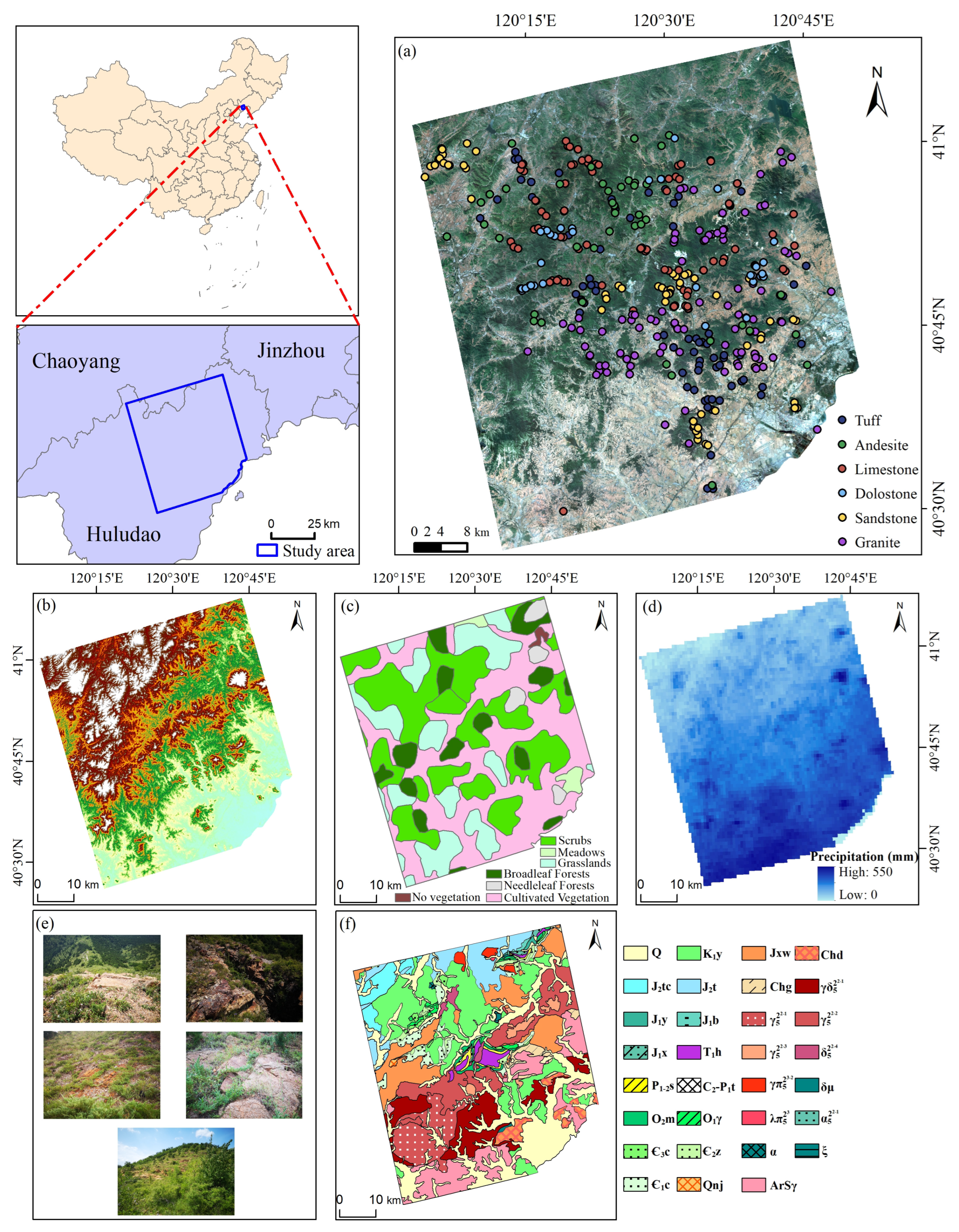
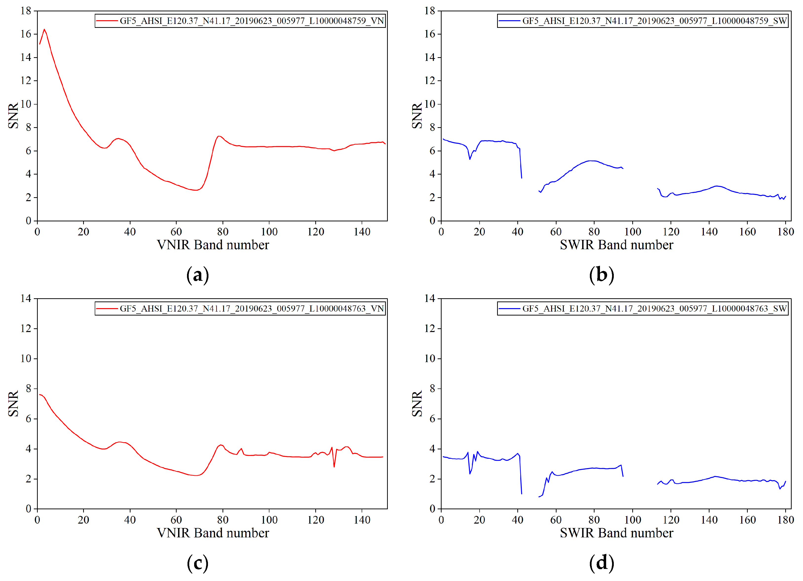
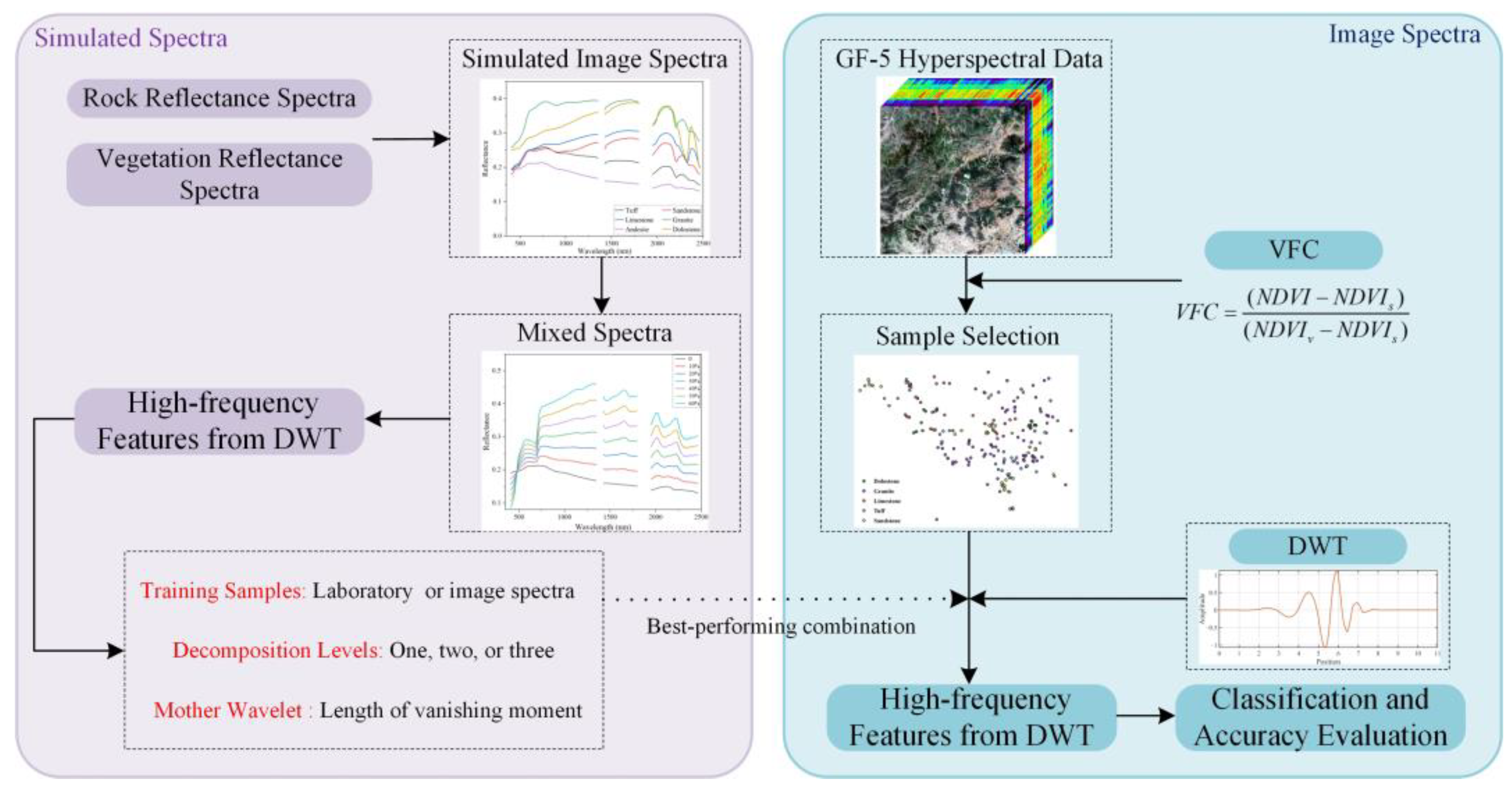
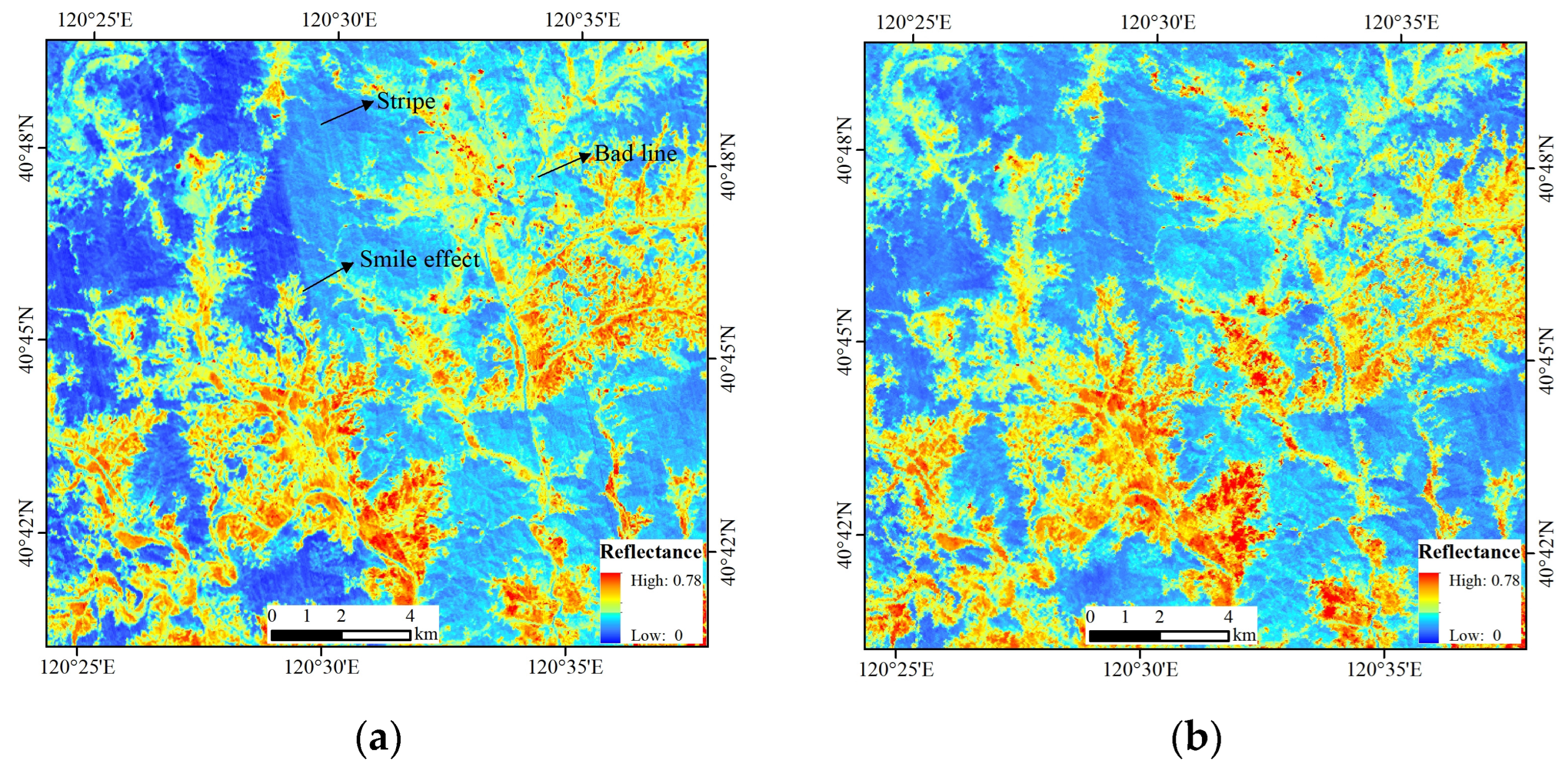
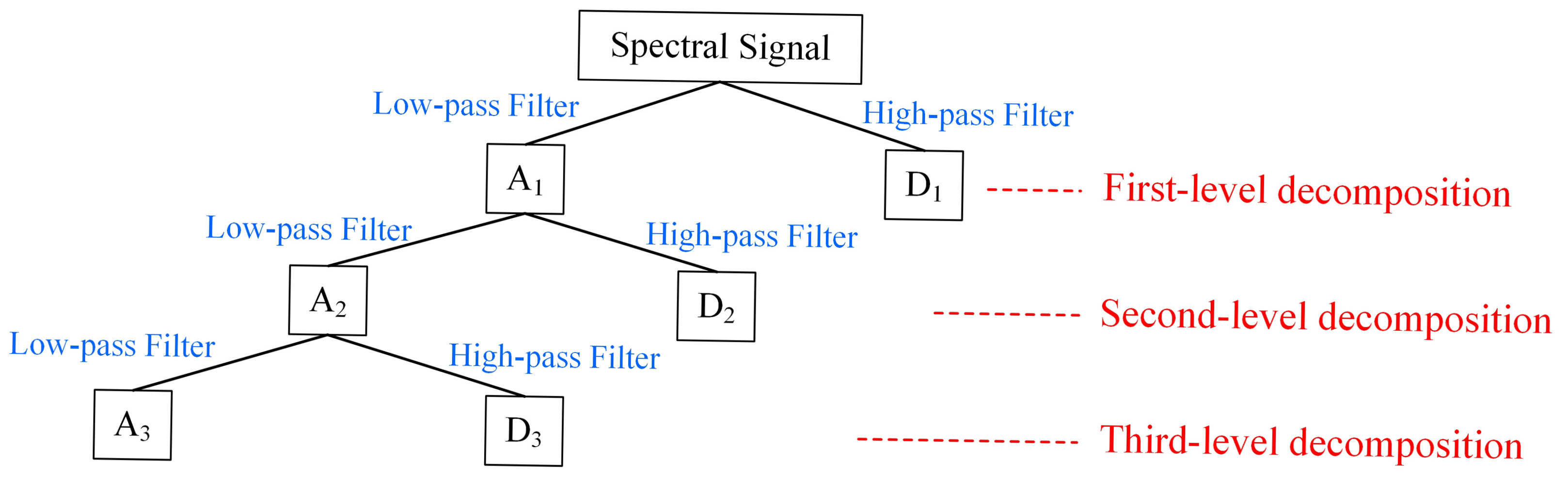
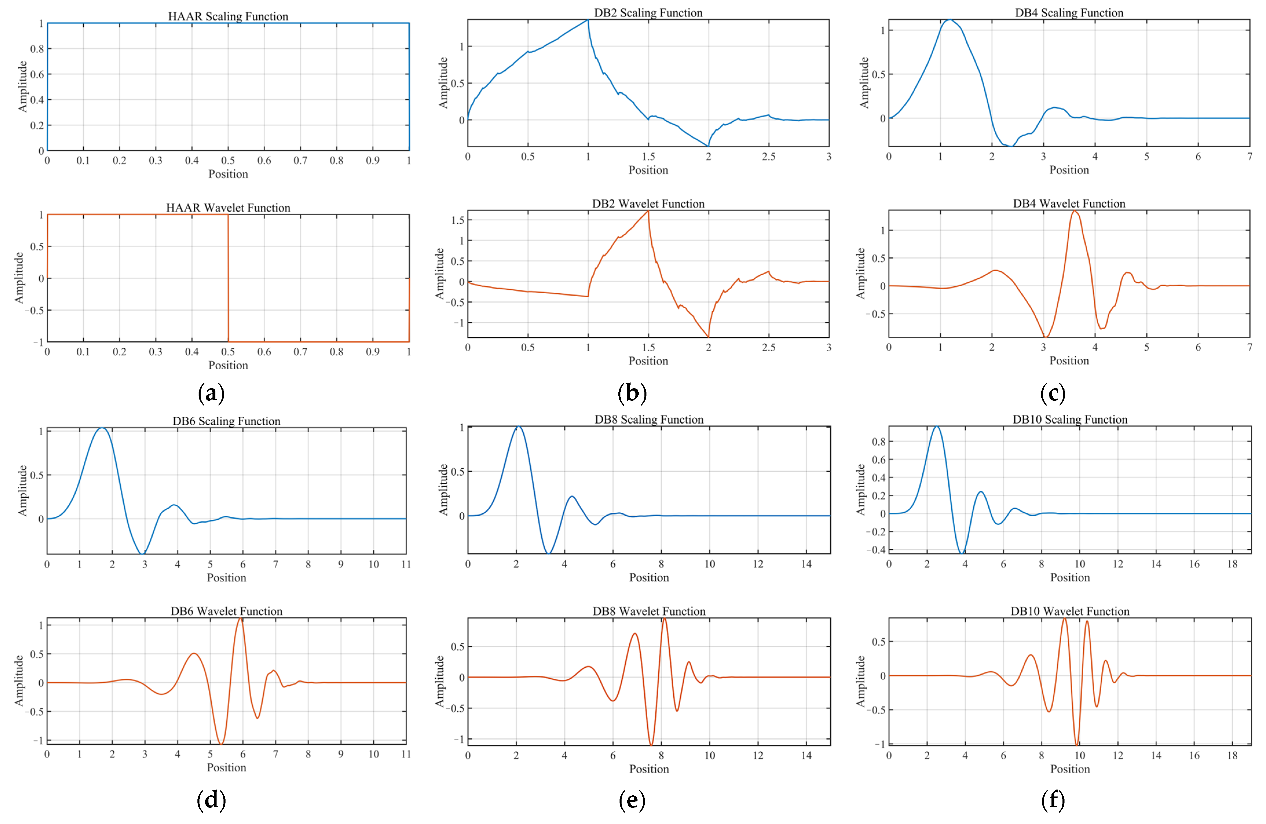
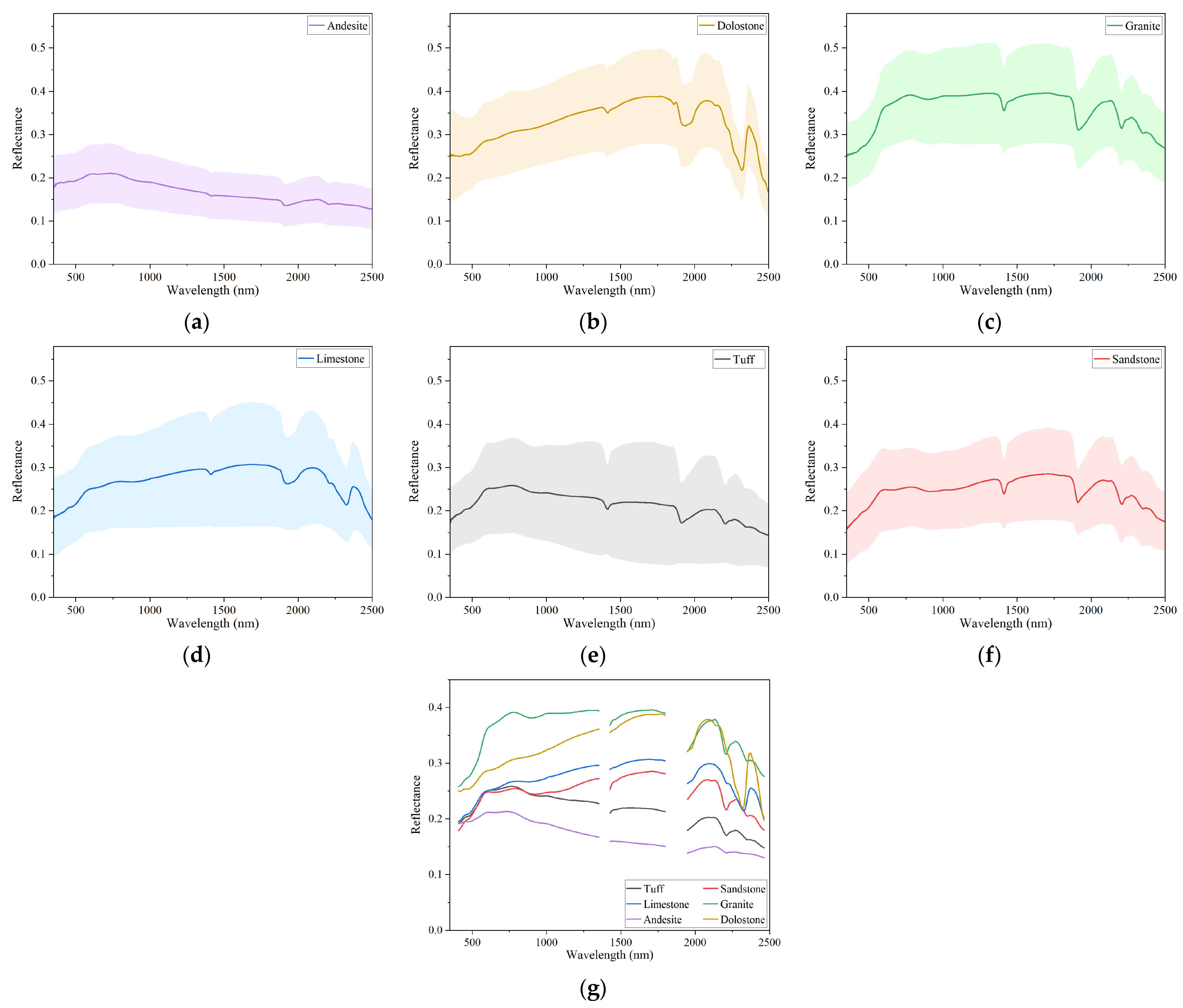
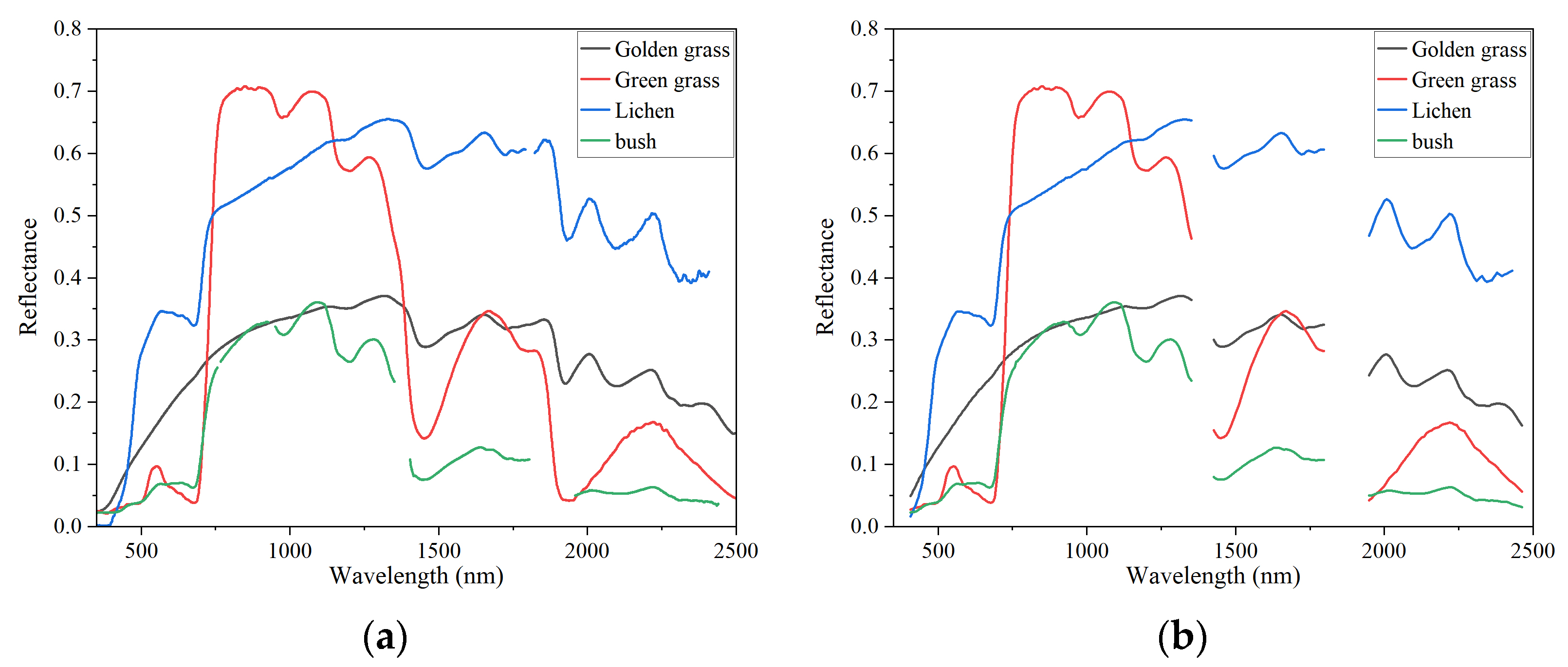
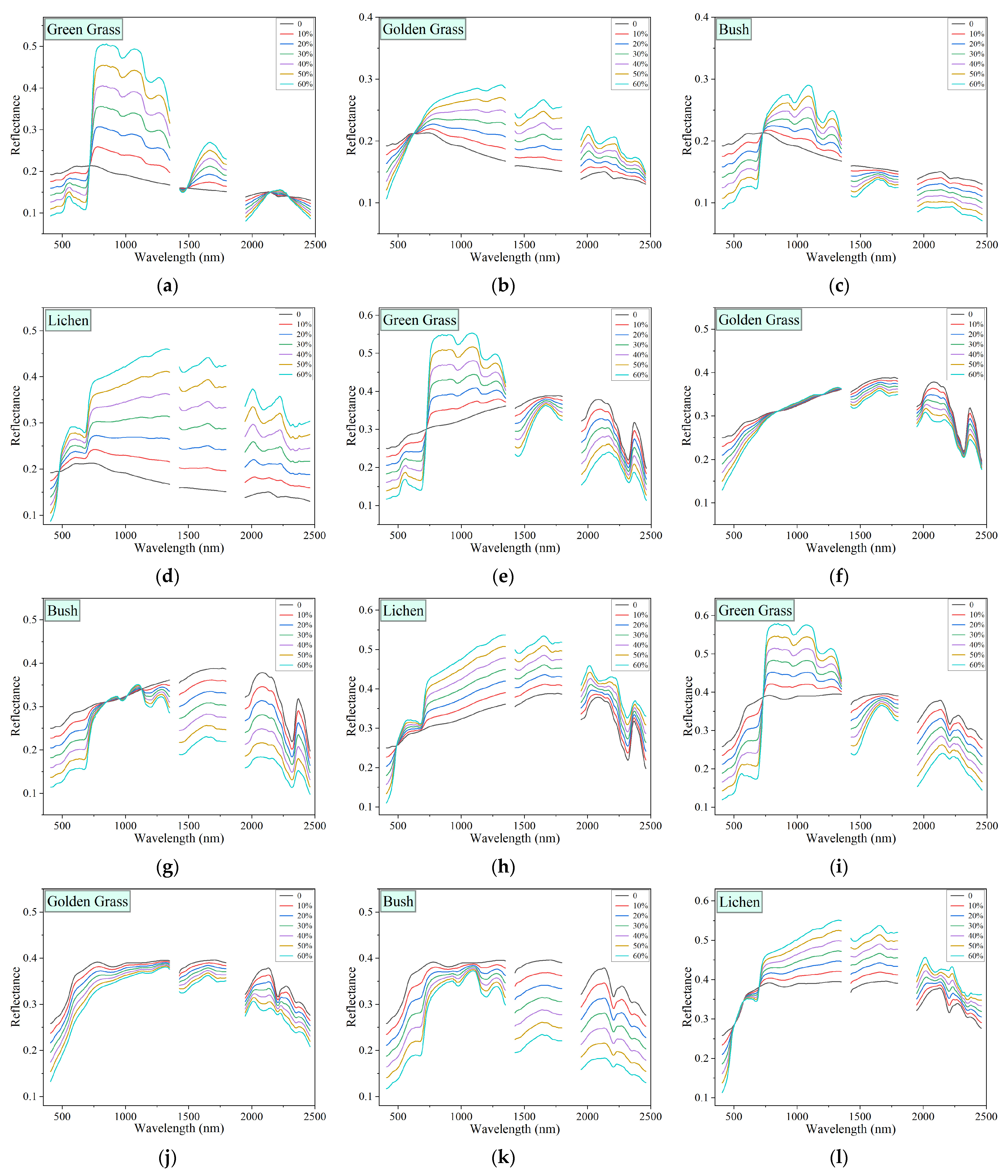
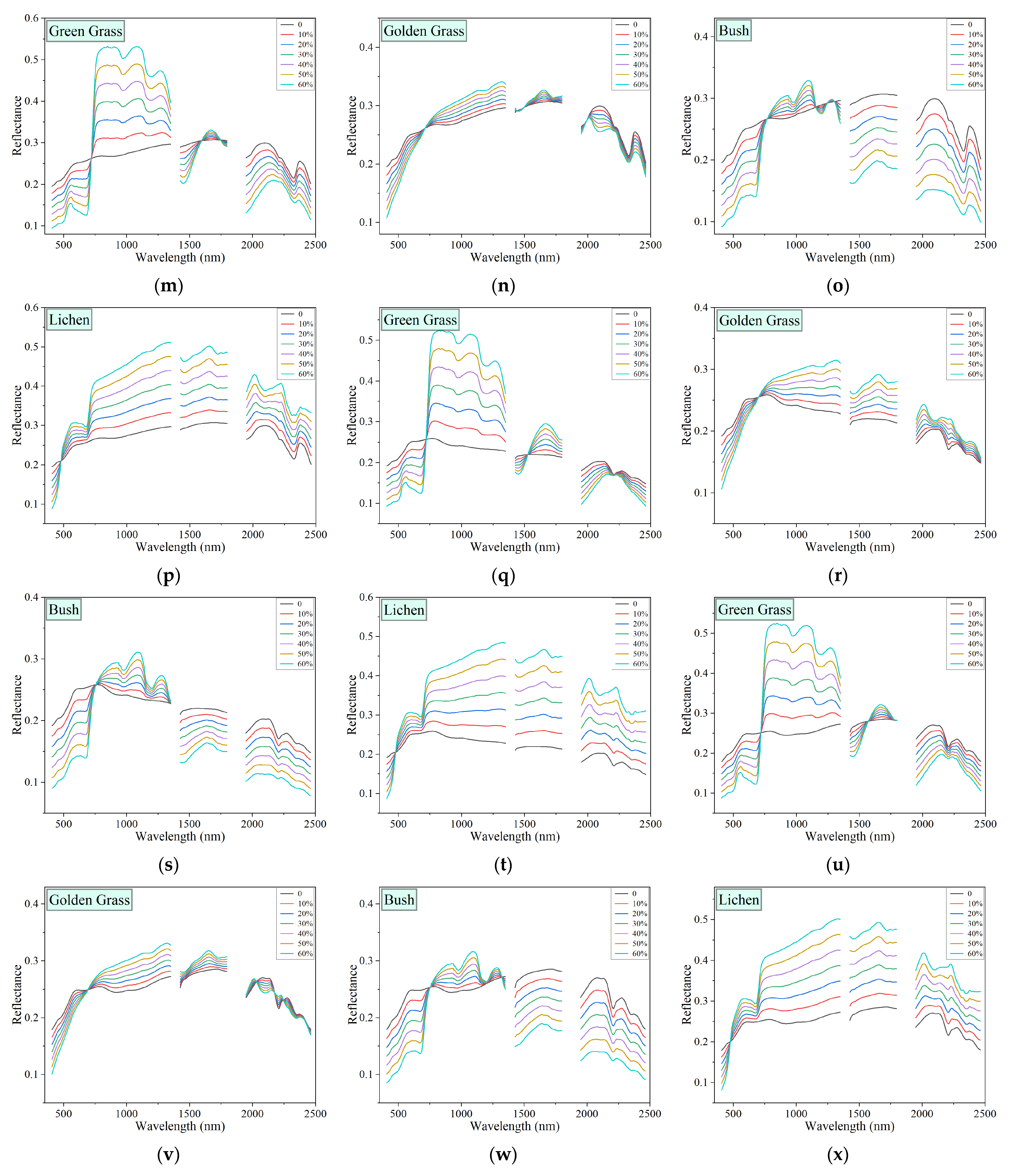
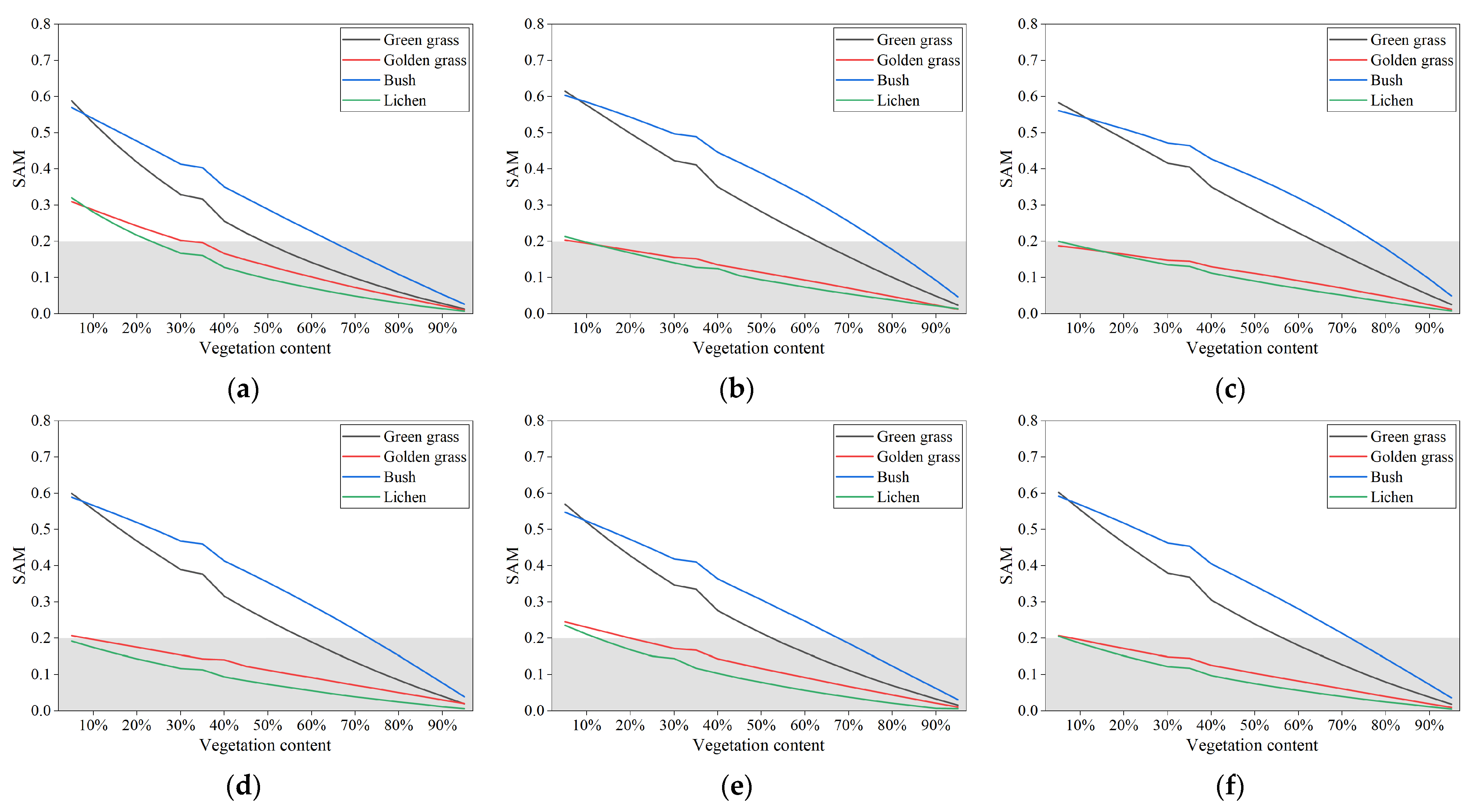
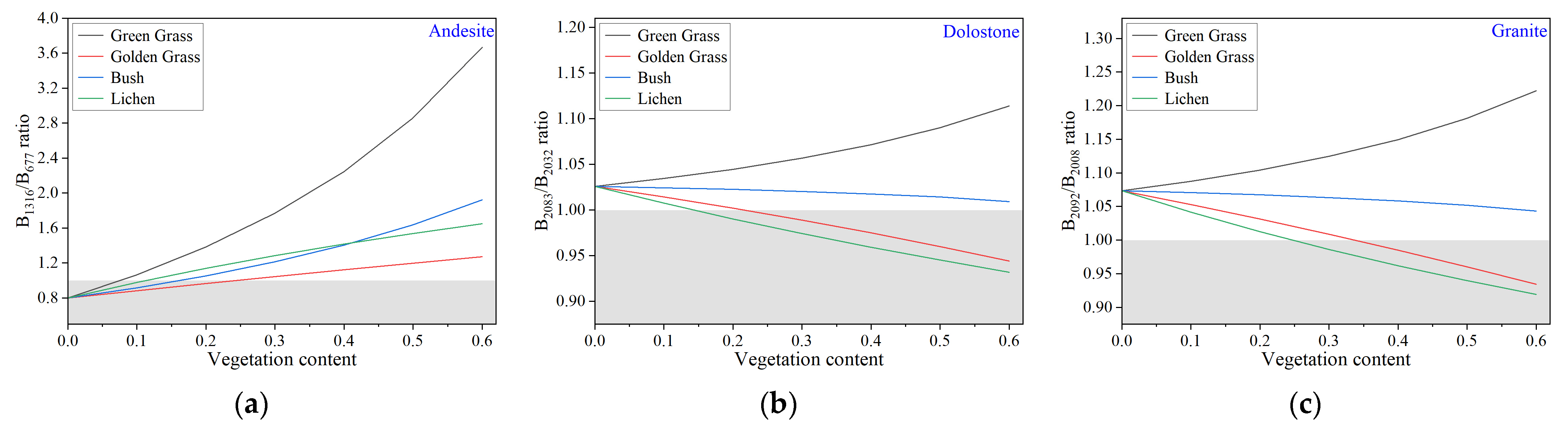
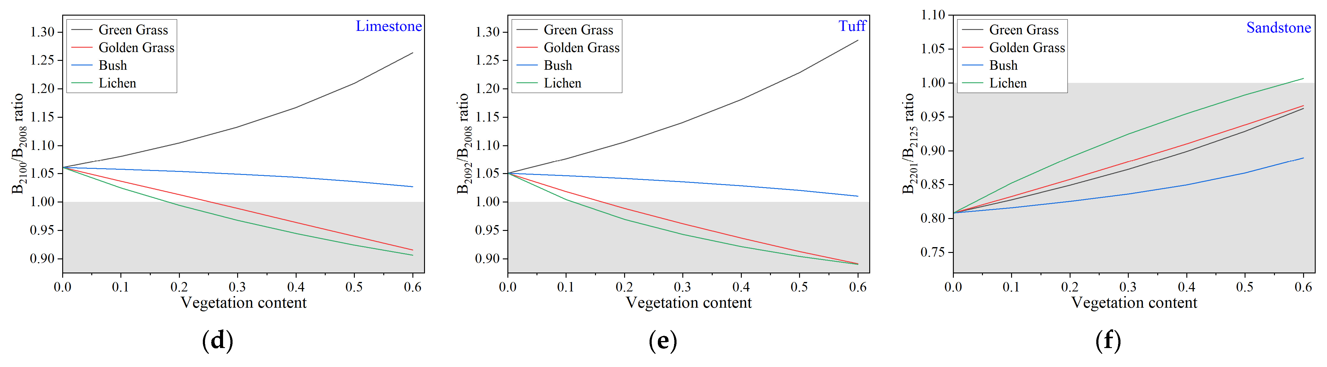
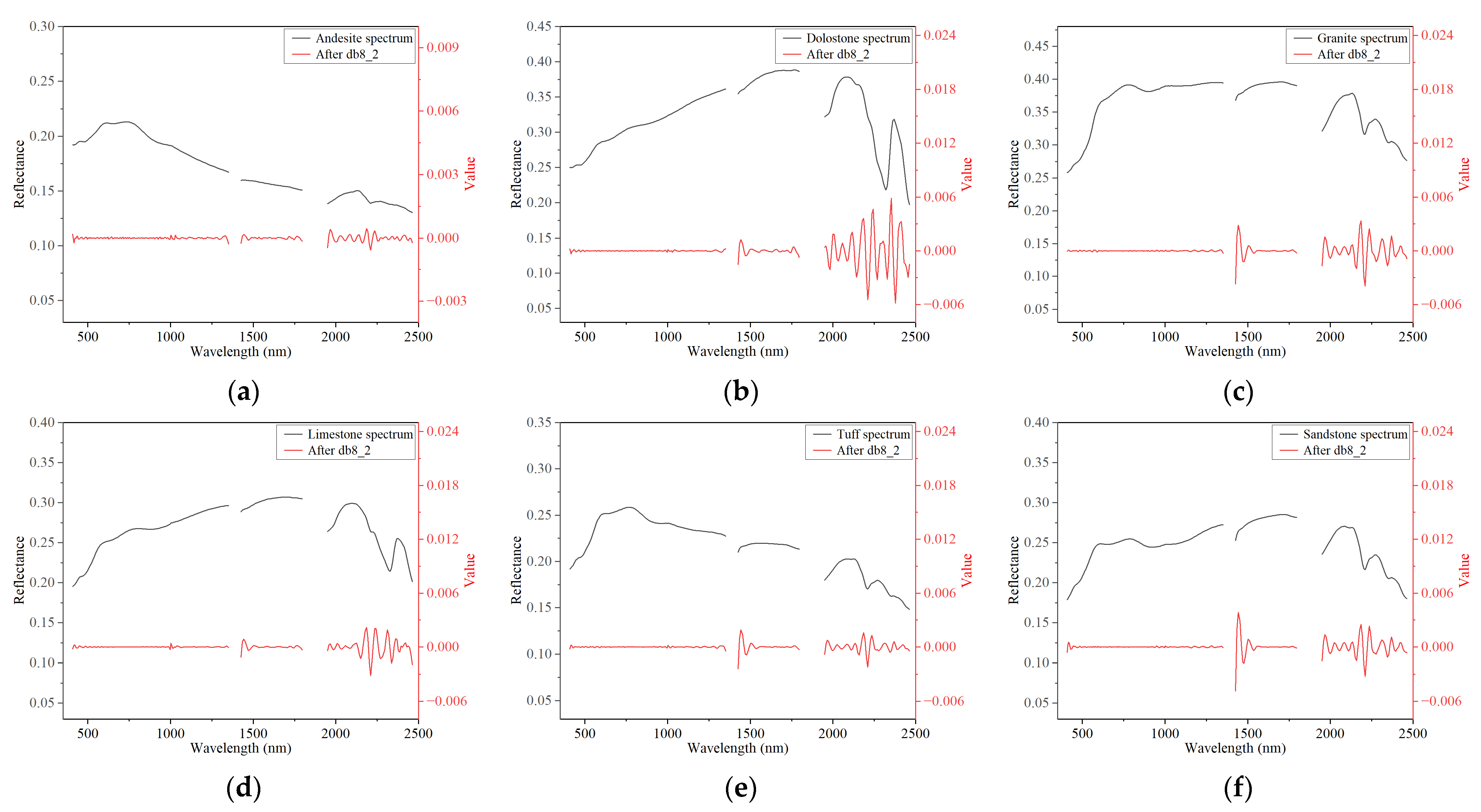
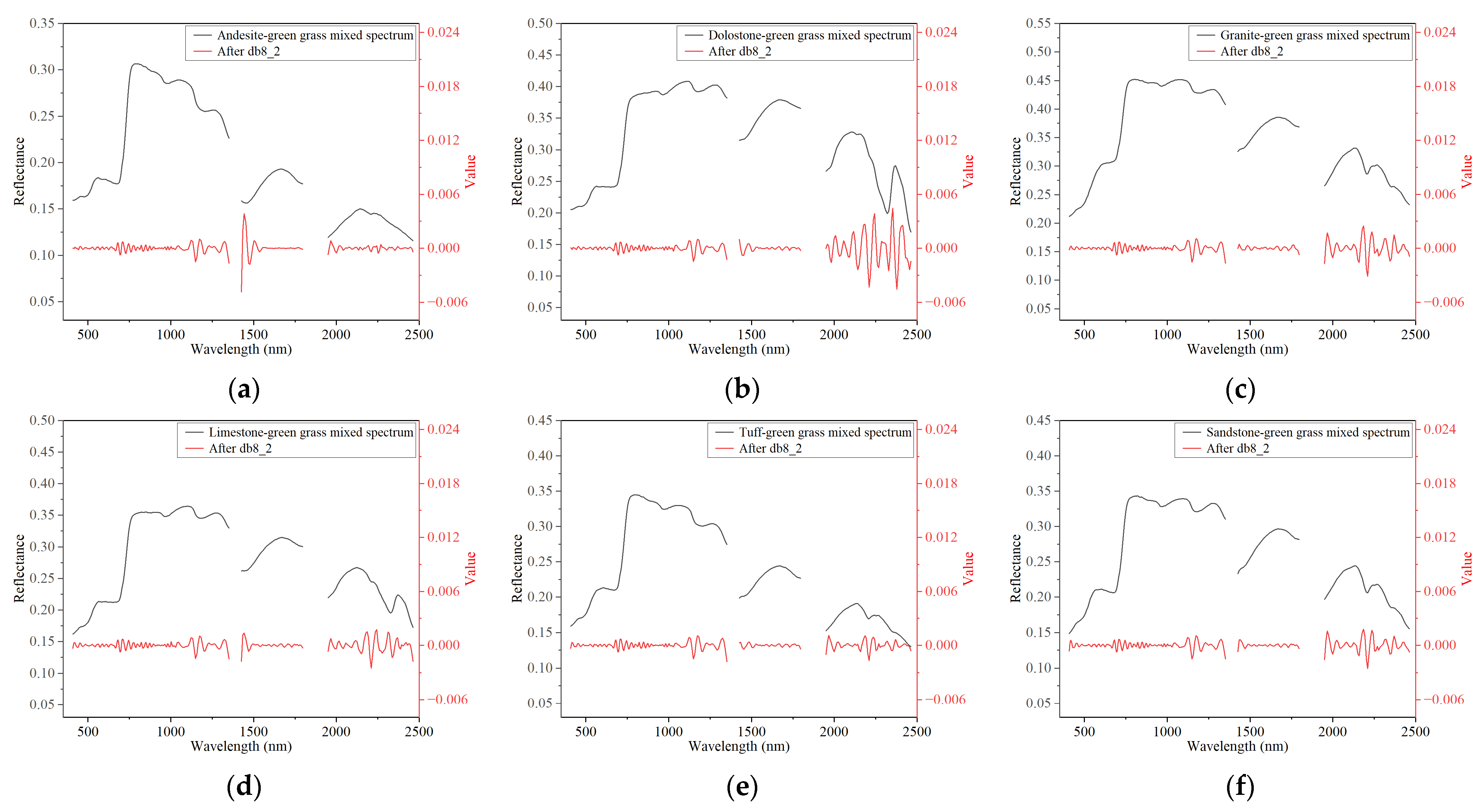
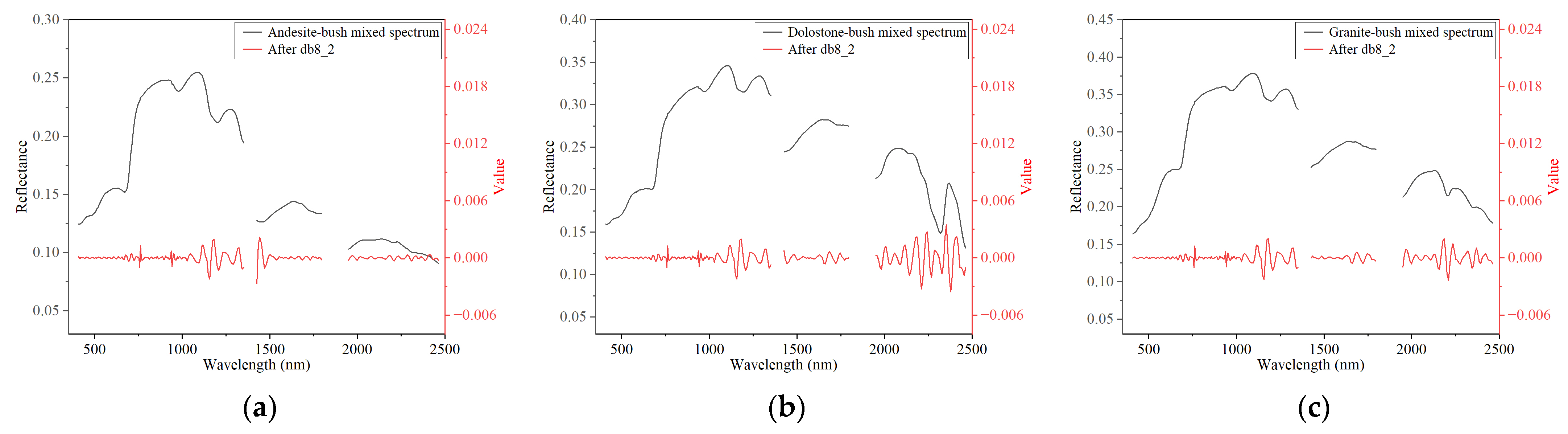
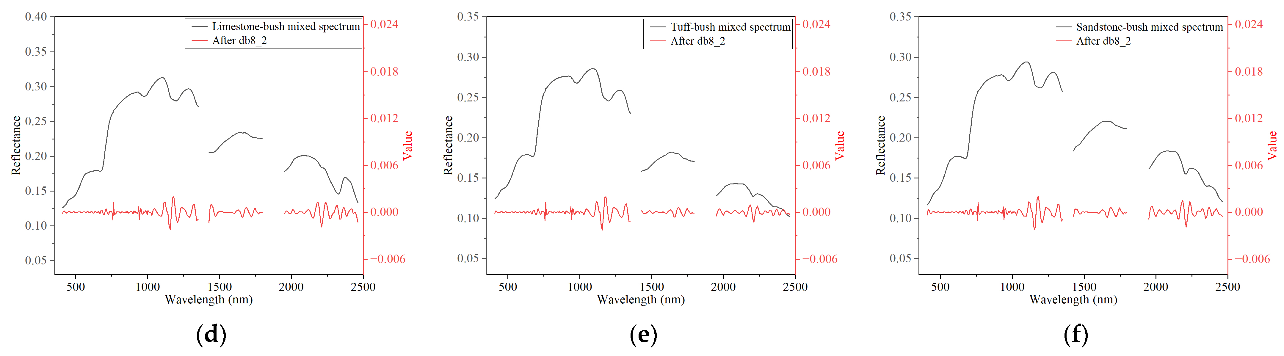
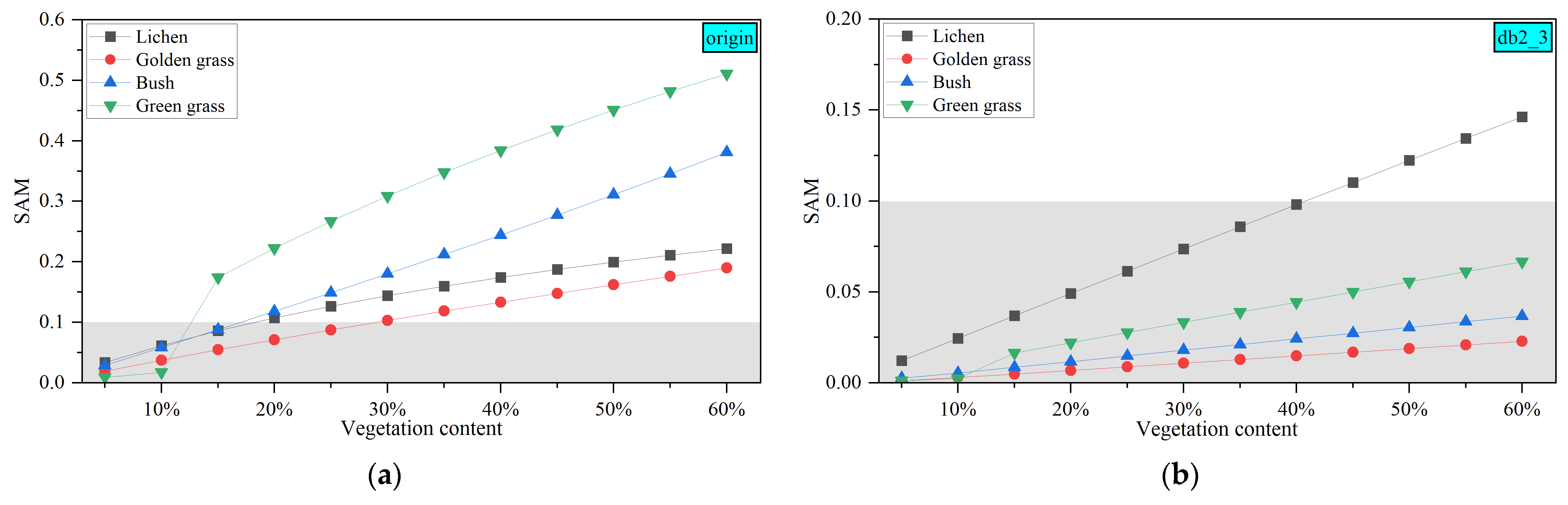
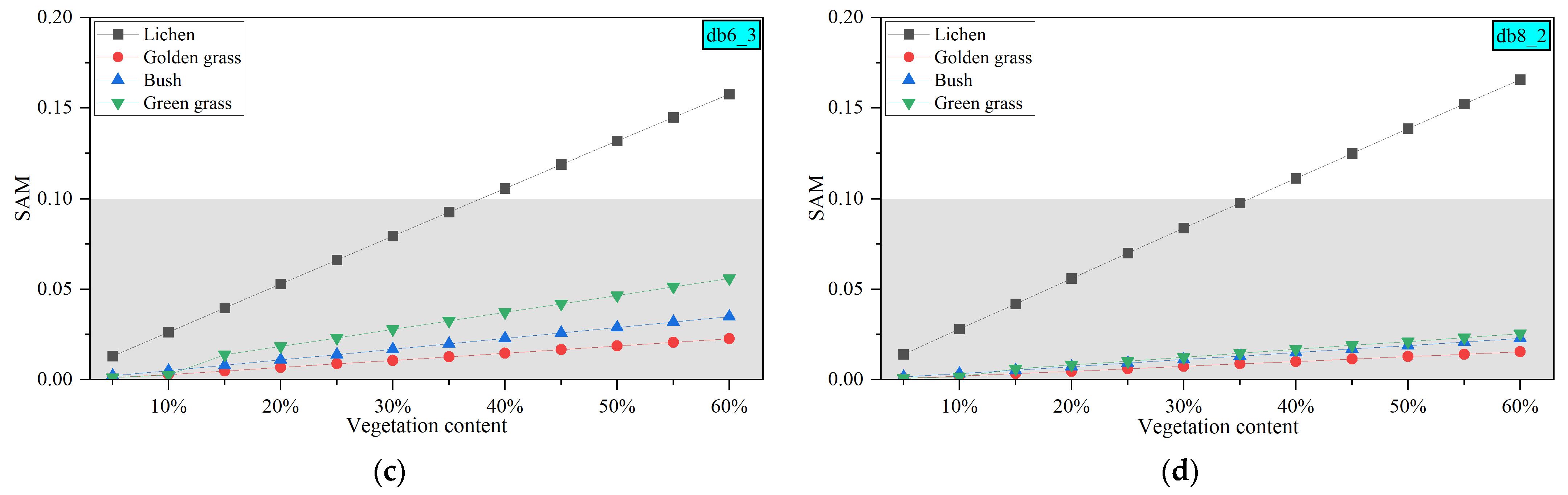
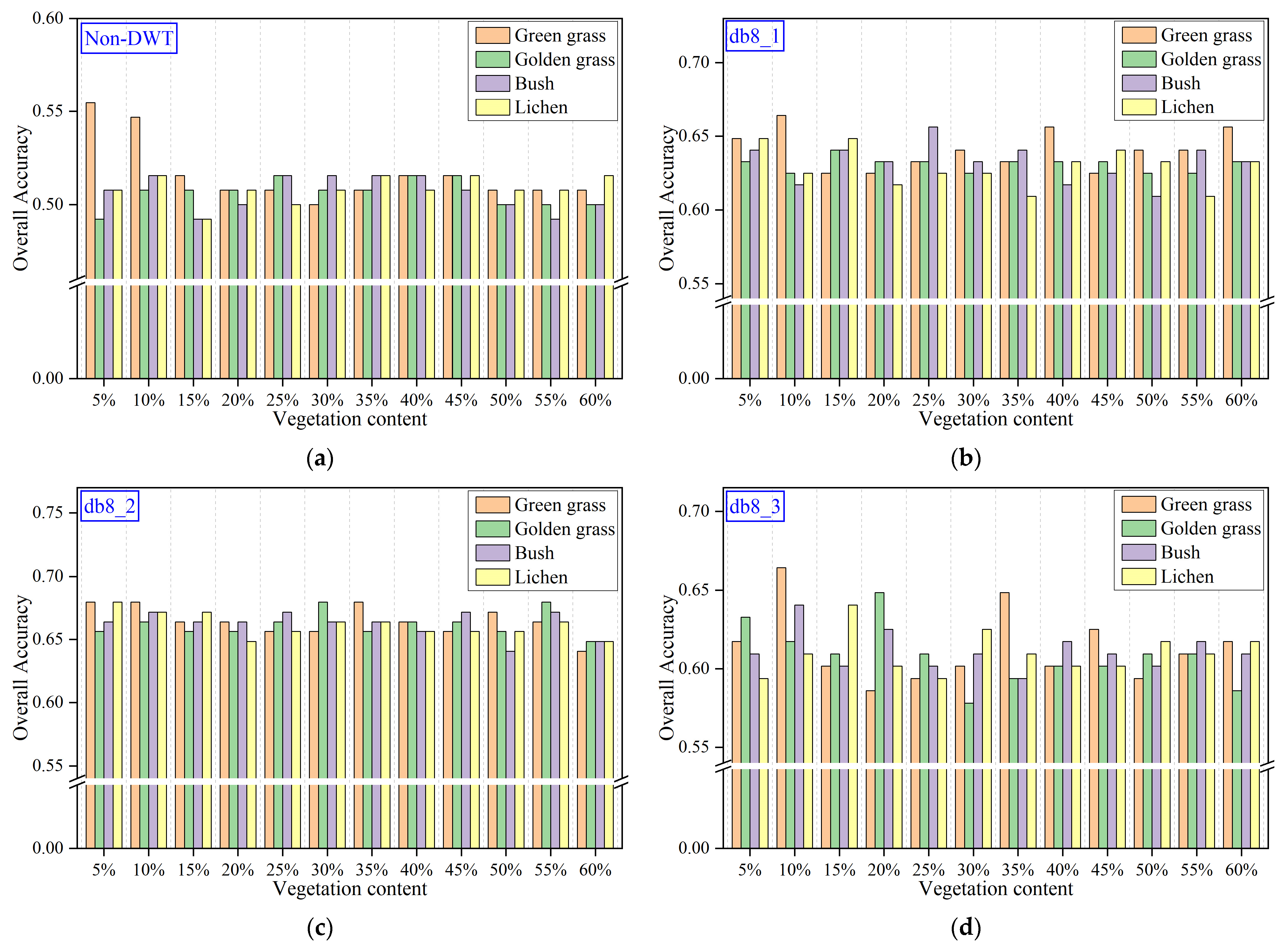
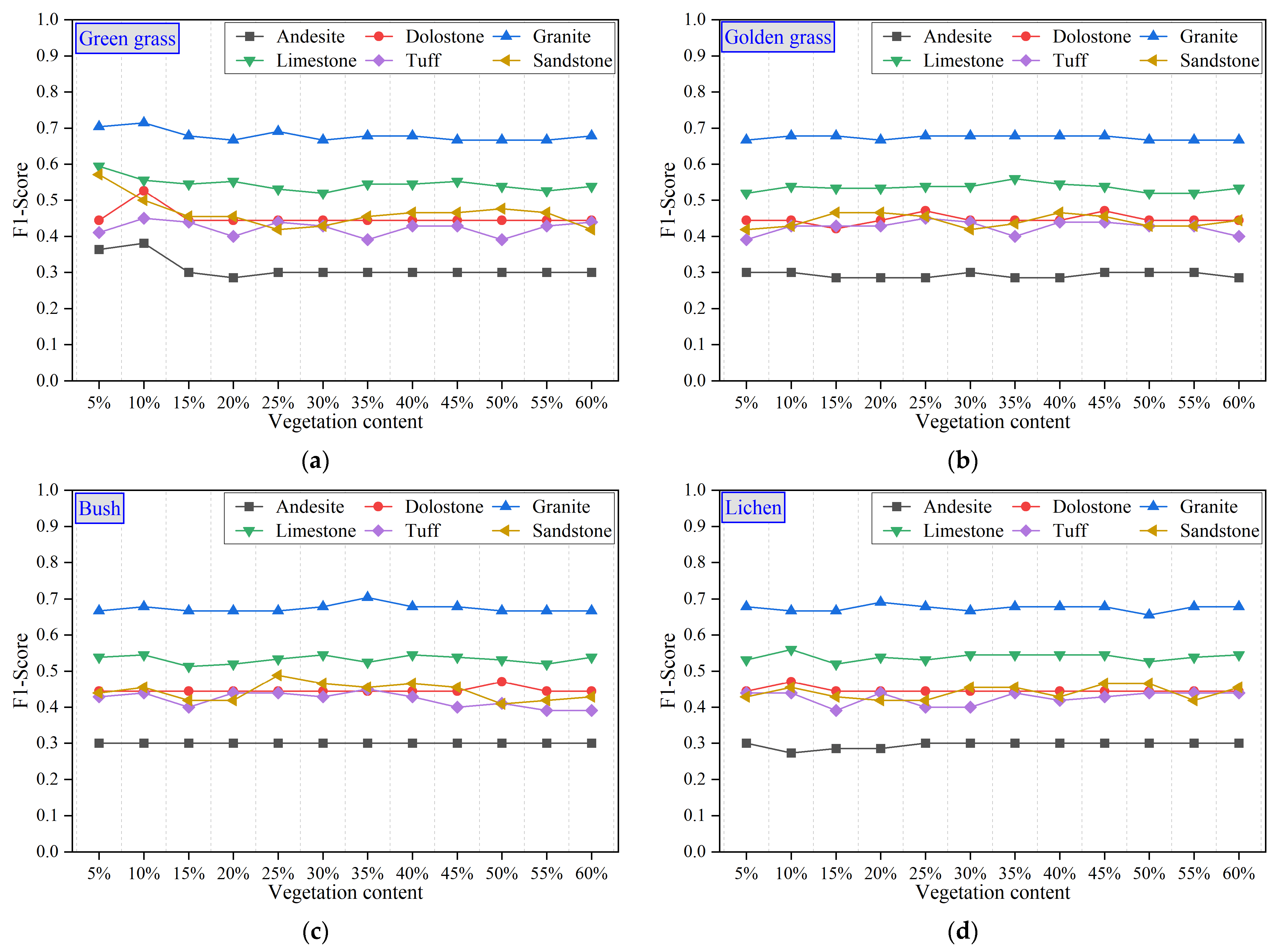
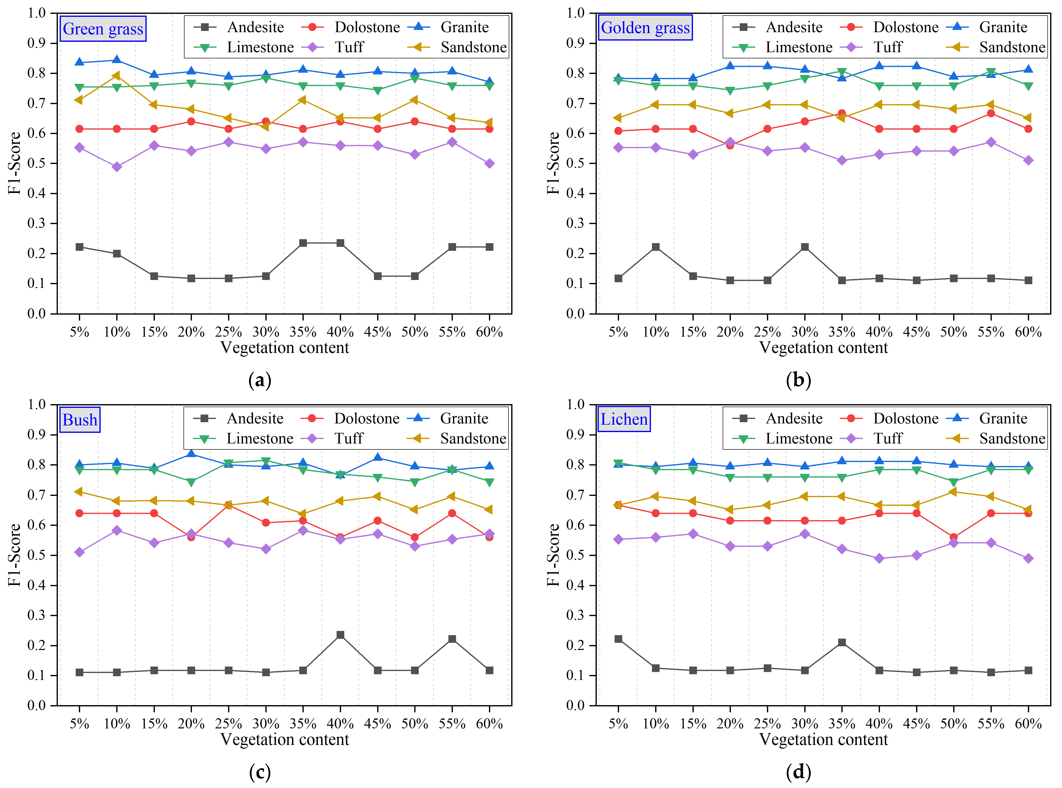
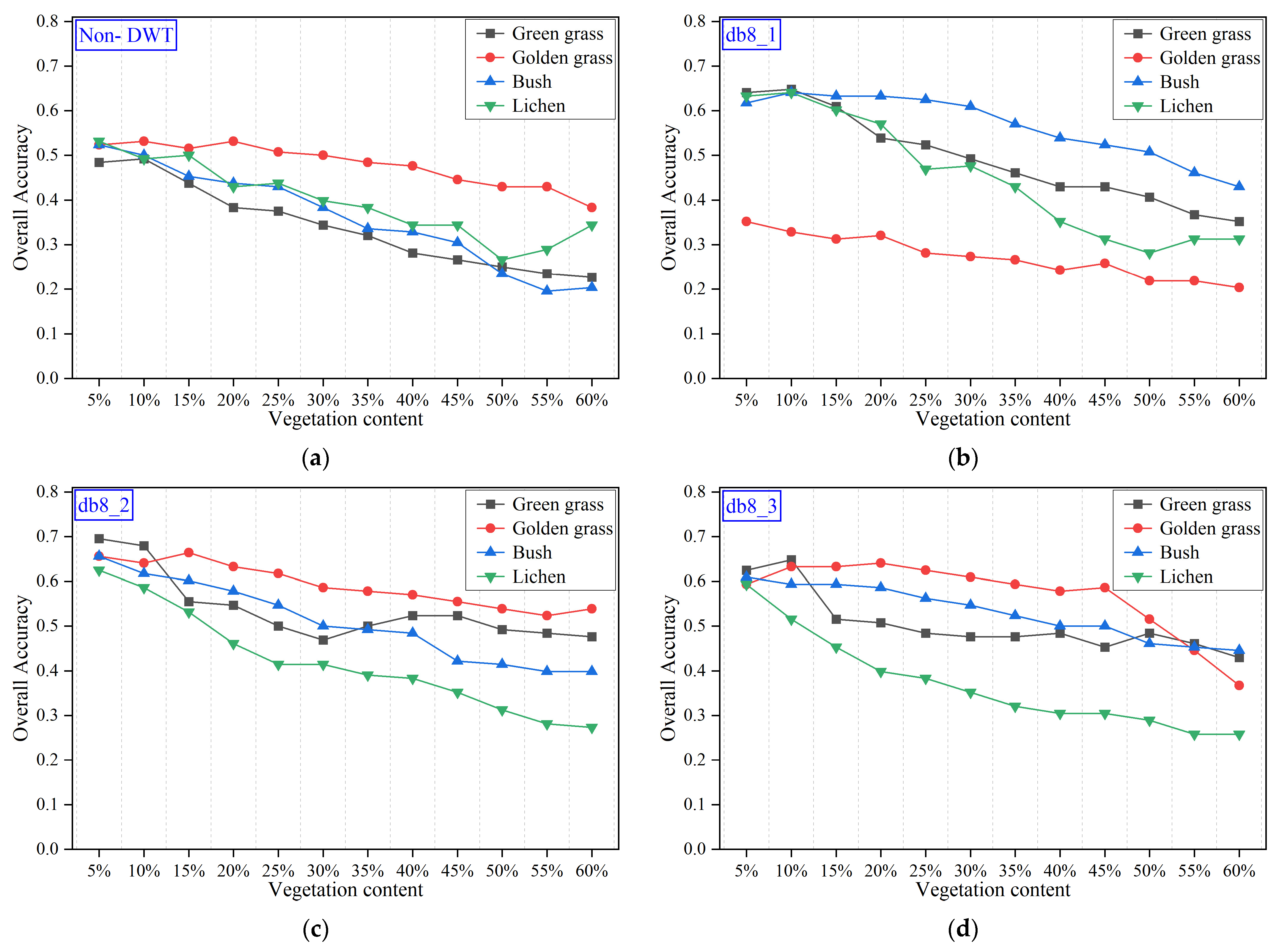
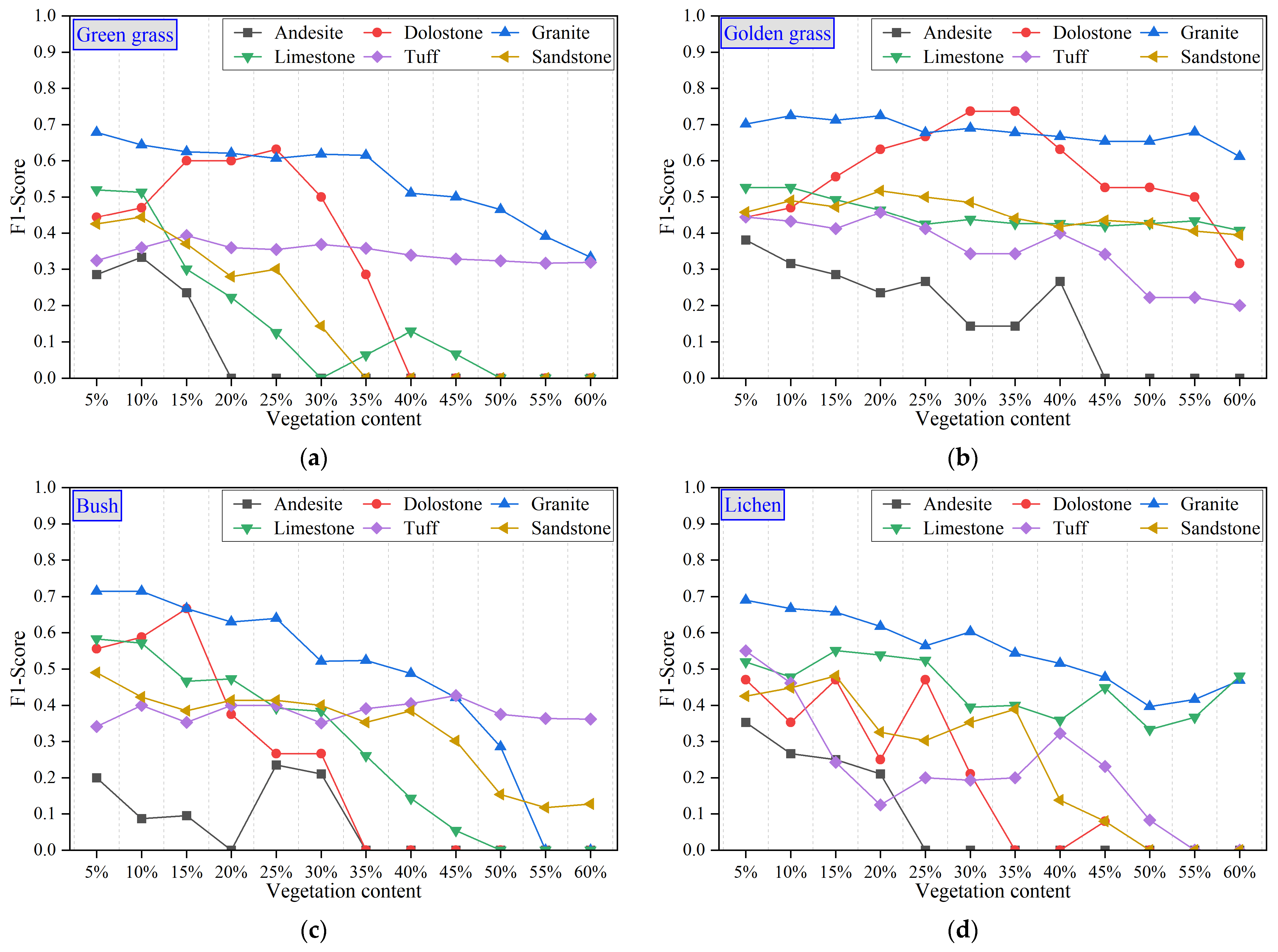
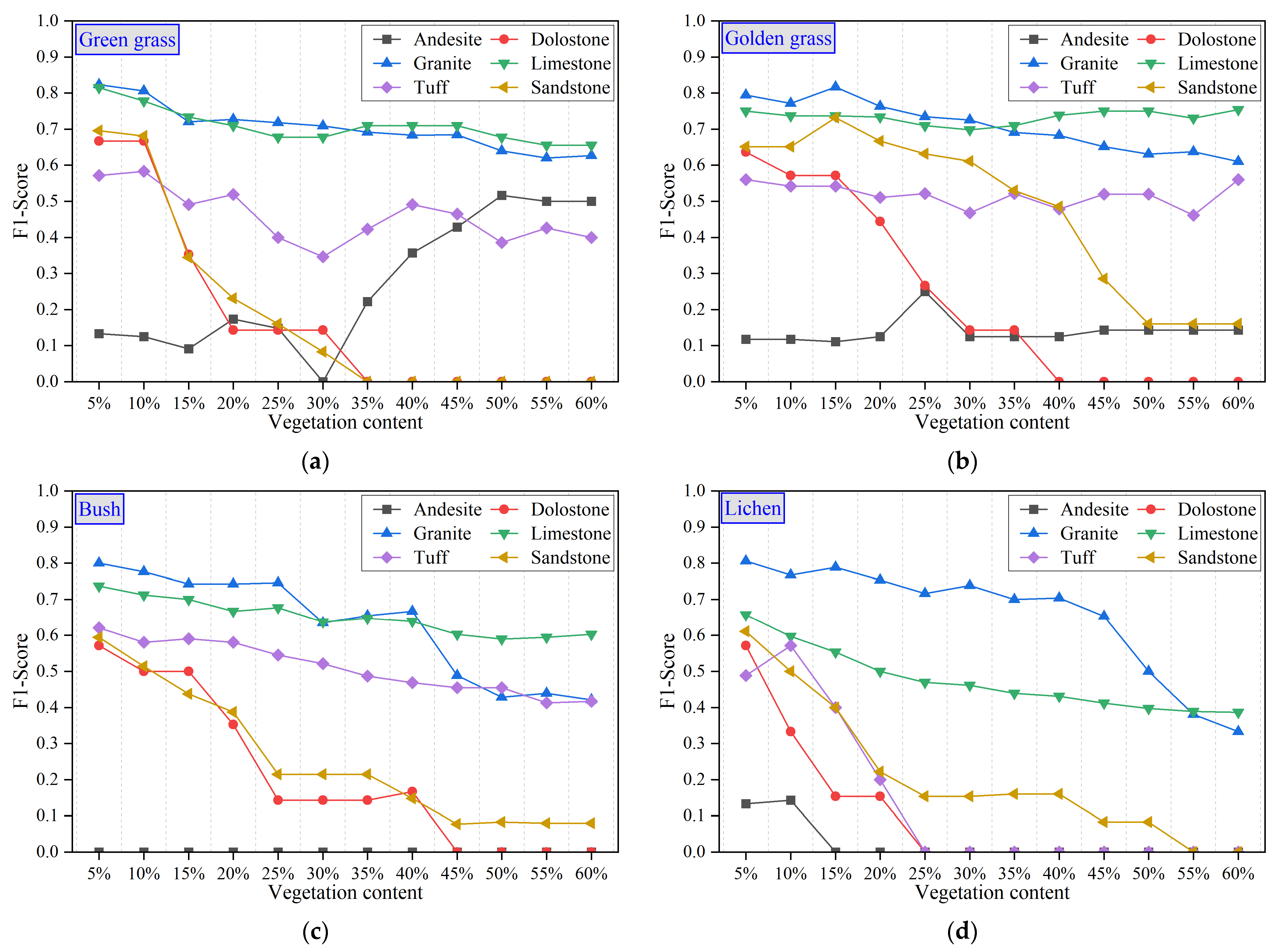

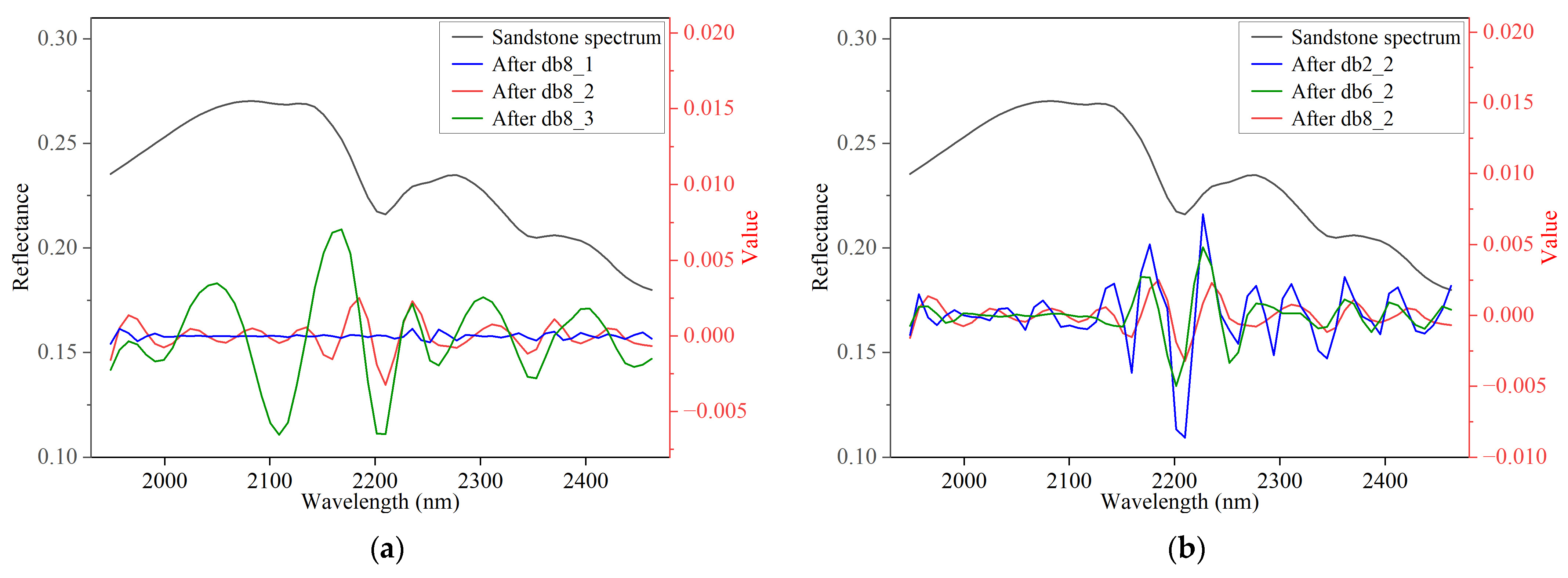
Disclaimer/Publisher’s Note: The statements, opinions and data contained in all publications are solely those of the individual author(s) and contributor(s) and not of MDPI and/or the editor(s). MDPI and/or the editor(s) disclaim responsibility for any injury to people or property resulting from any ideas, methods, instructions or products referred to in the content. |
© 2025 by the authors. Licensee MDPI, Basel, Switzerland. This article is an open access article distributed under the terms and conditions of the Creative Commons Attribution (CC BY) license (https://creativecommons.org/licenses/by/4.0/).