

Kohler-Polarization Sensor for Glint Removal in Water-Leaving Radiance Measurement


Abstract
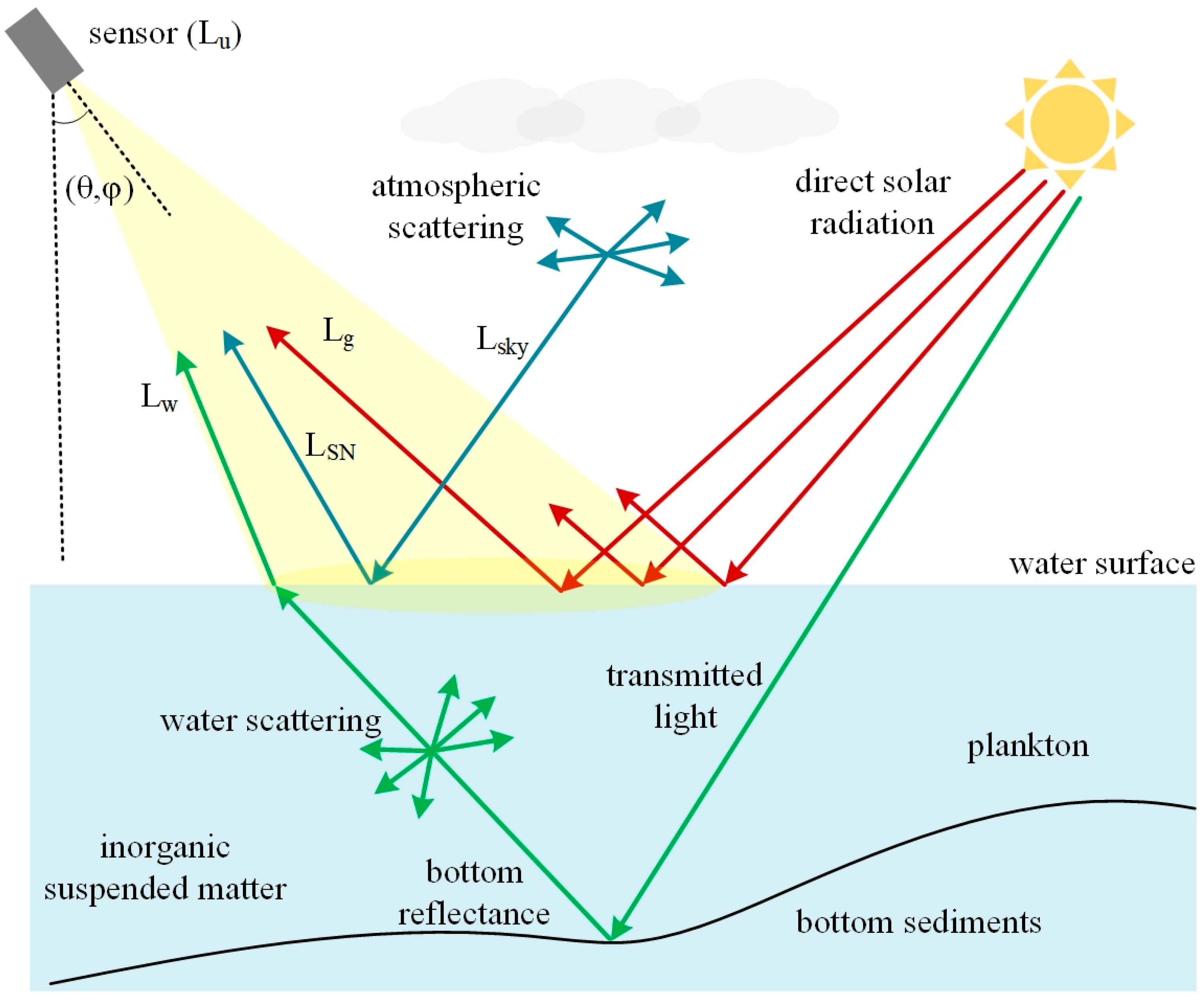
1. Introduction
- Observation geometry.
- Solar elevation/azimuth angles.
- Cloud distribution patterns.
- Wind speed and direction.
- Practical difficulties in comprehensive environmental parameter monitoring.
- Limitations in existing glint correction algorithms to handle natural variability.
2. Related Works
3. The Design and Calibration of the System
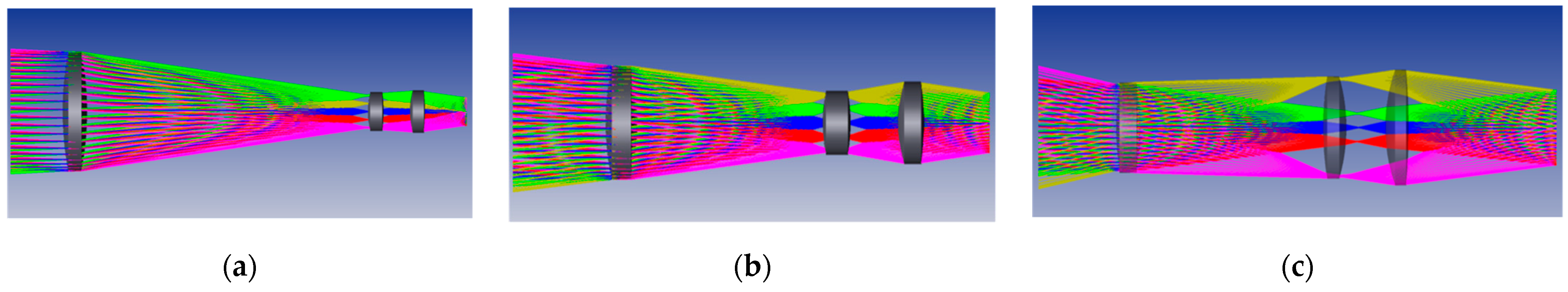
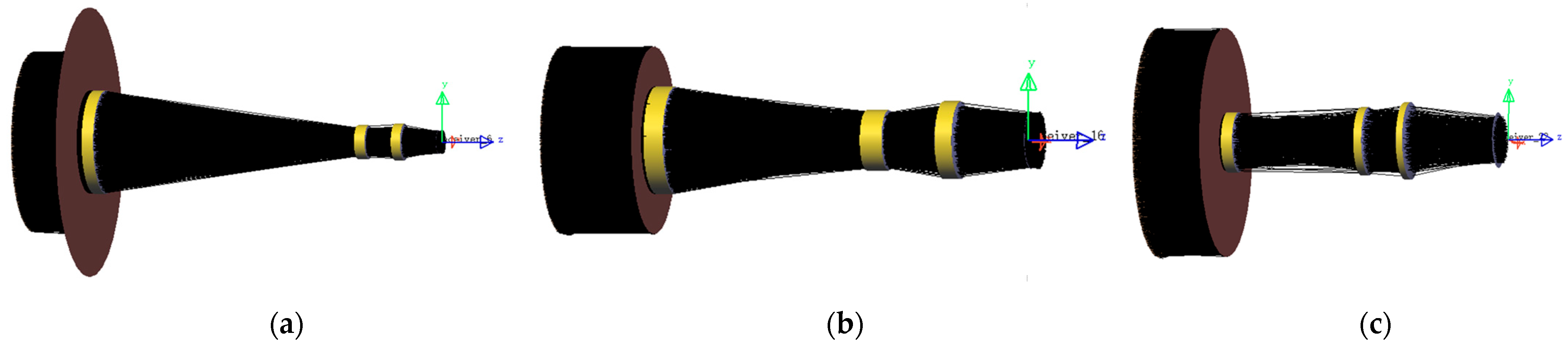
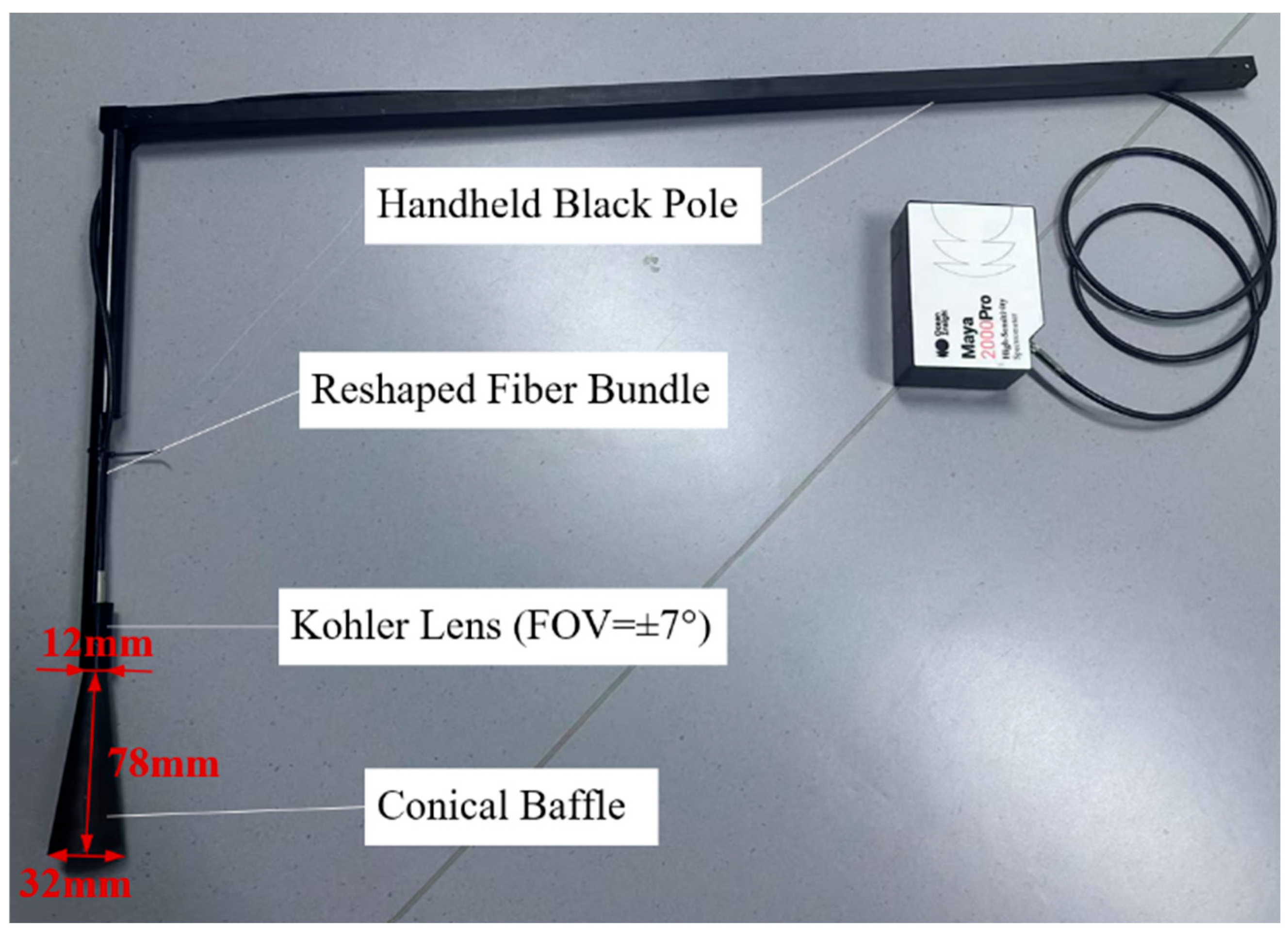
3.1. Specific Design and Test Methodology
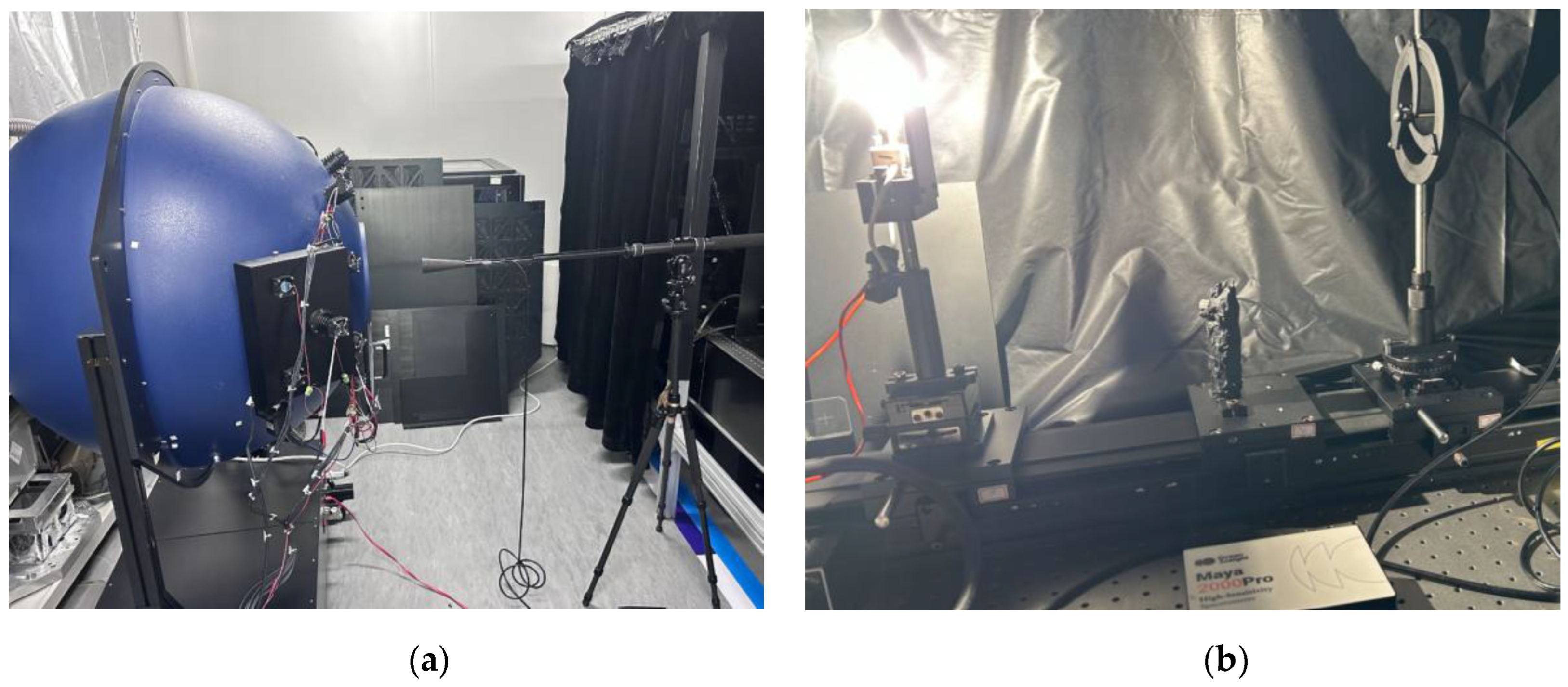
3.2. Laboratory Radiometric Calibration
4. Field Experiments and Results
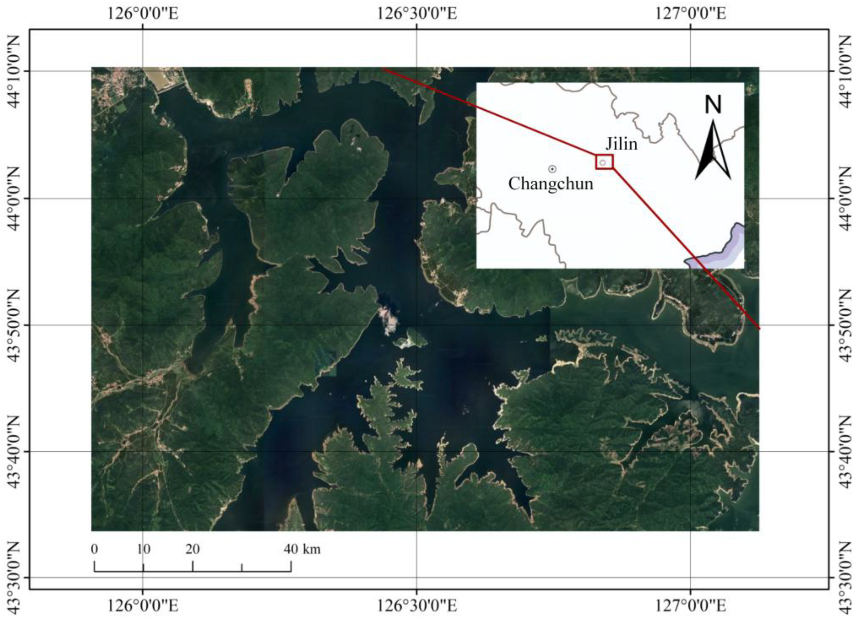
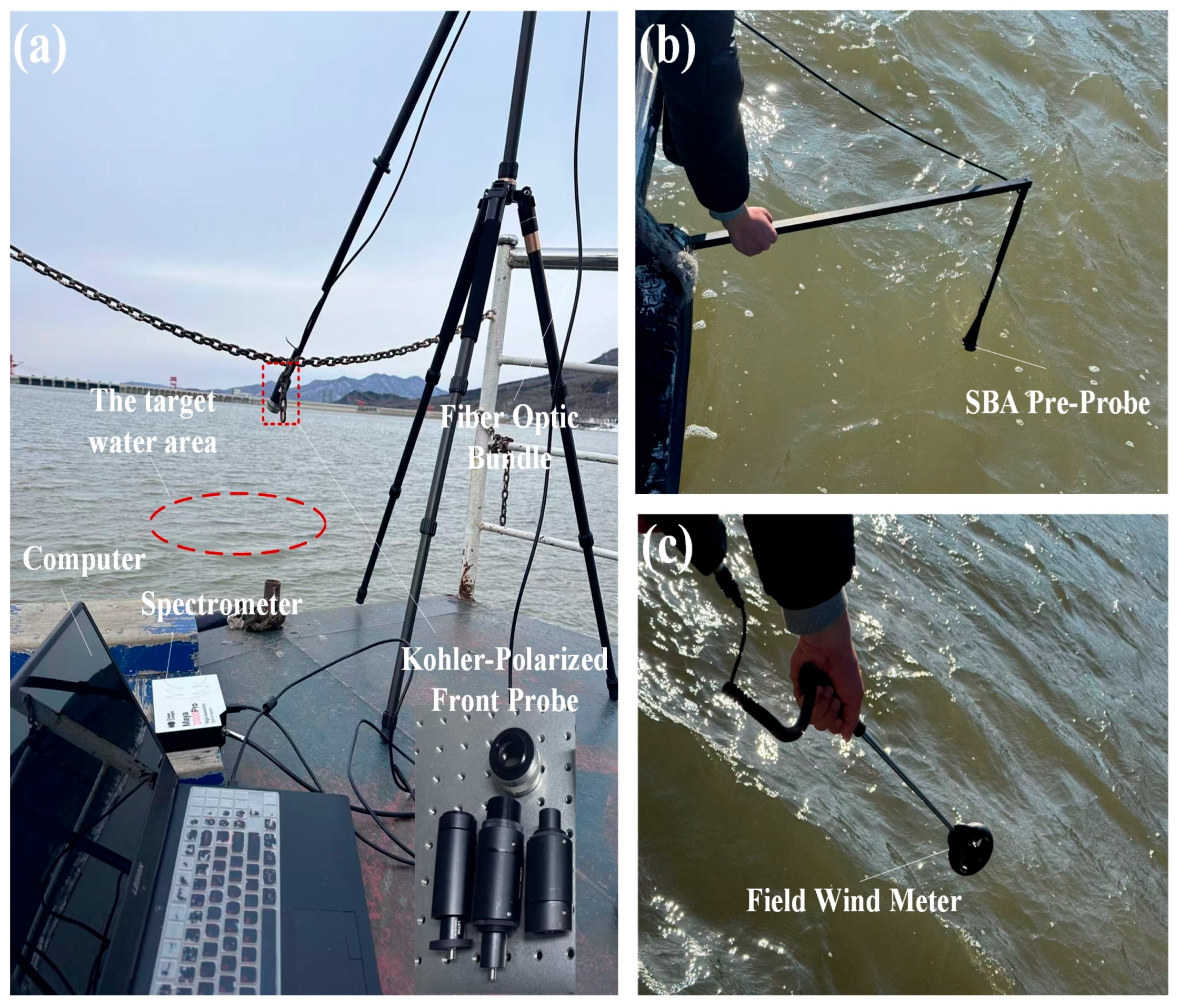
4.1. Field Experiments
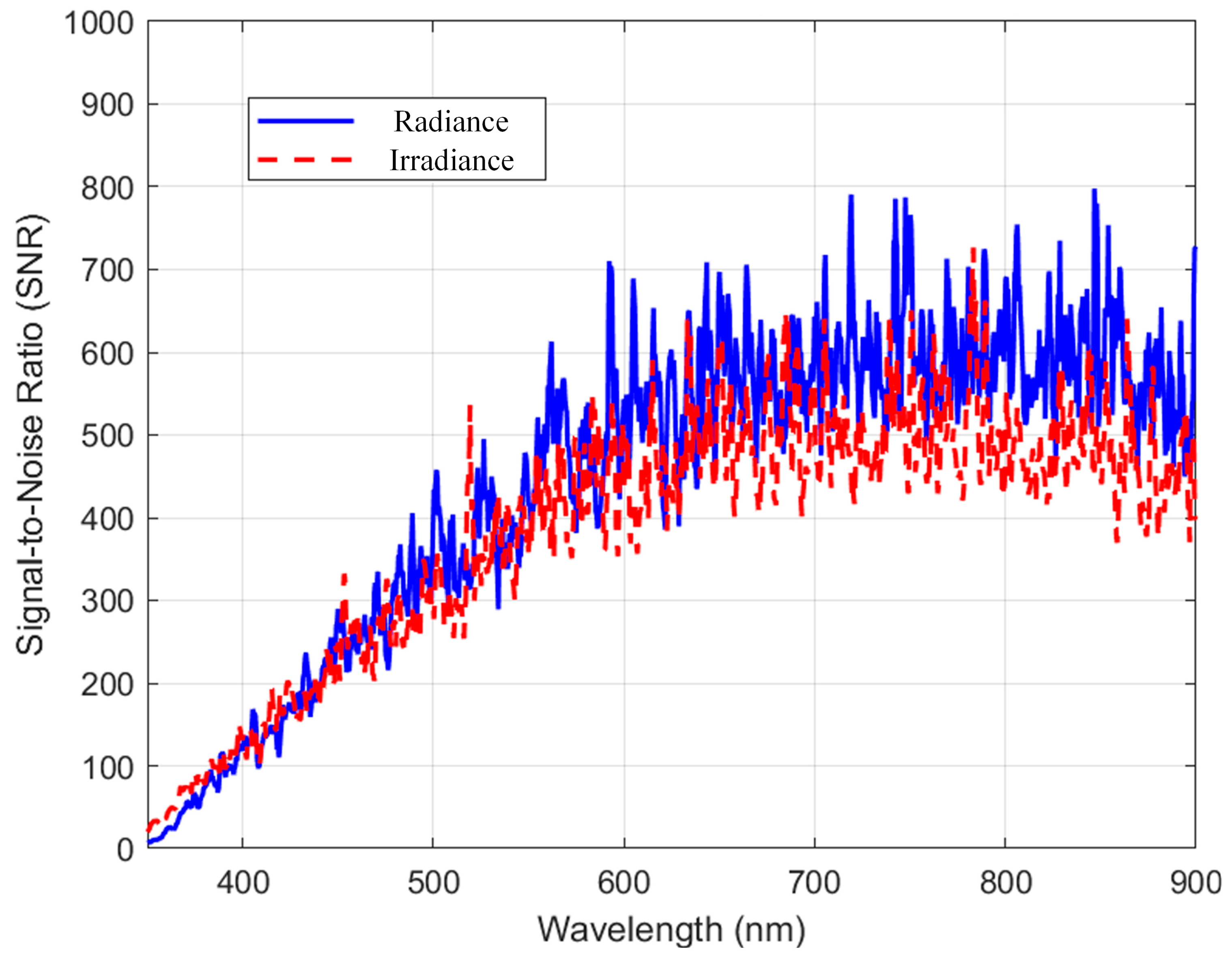
4.2. Test Results of System
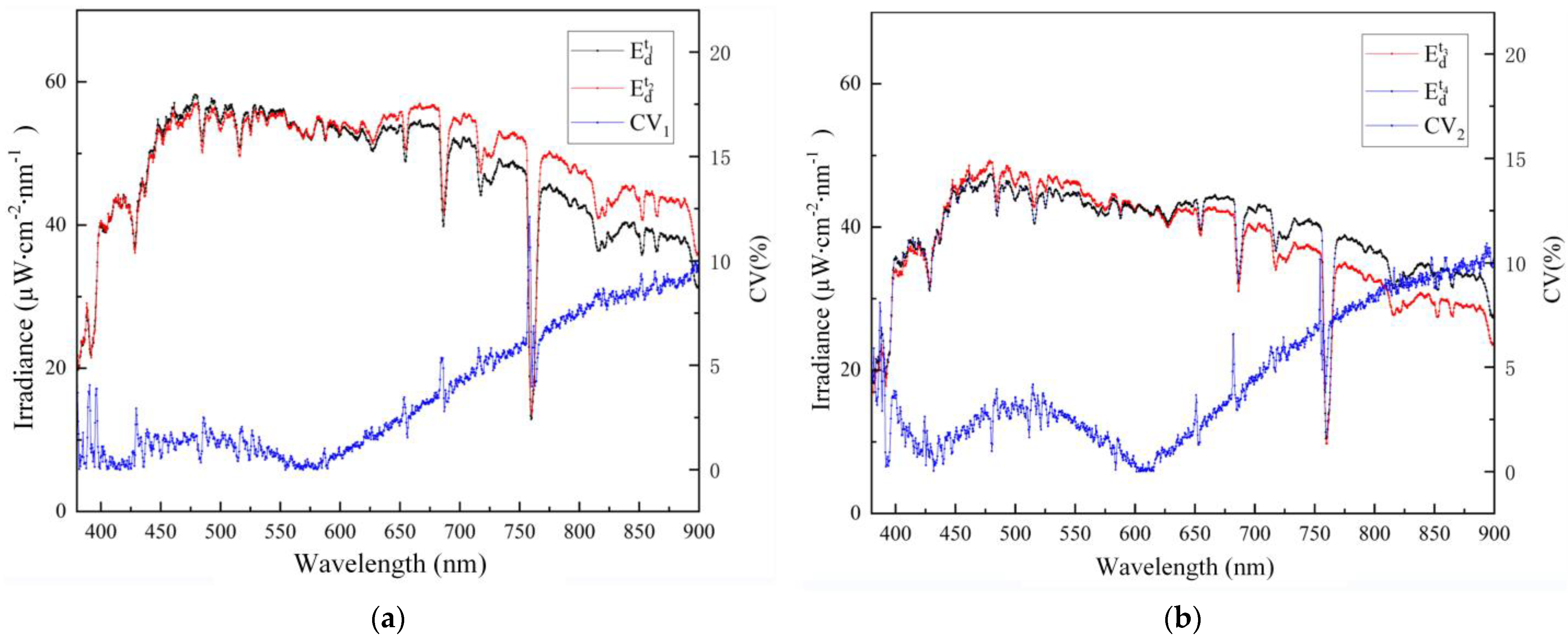
4.3. Measurement Results of Downwelling Irradiance at Water Surface
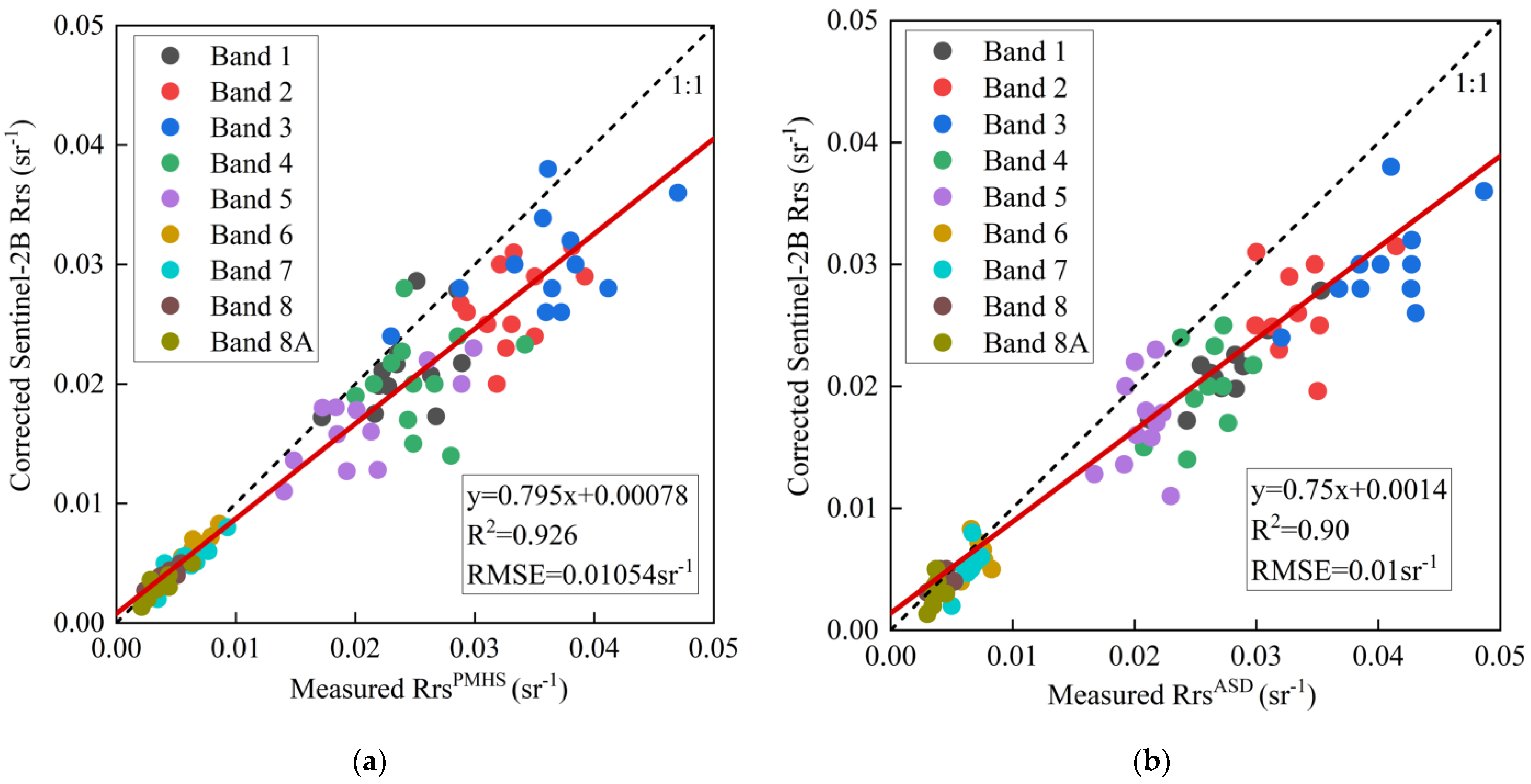
4.4. Cross Validation of Satellite Data
4.5. Measurement Results of Water-Leaving Radiance
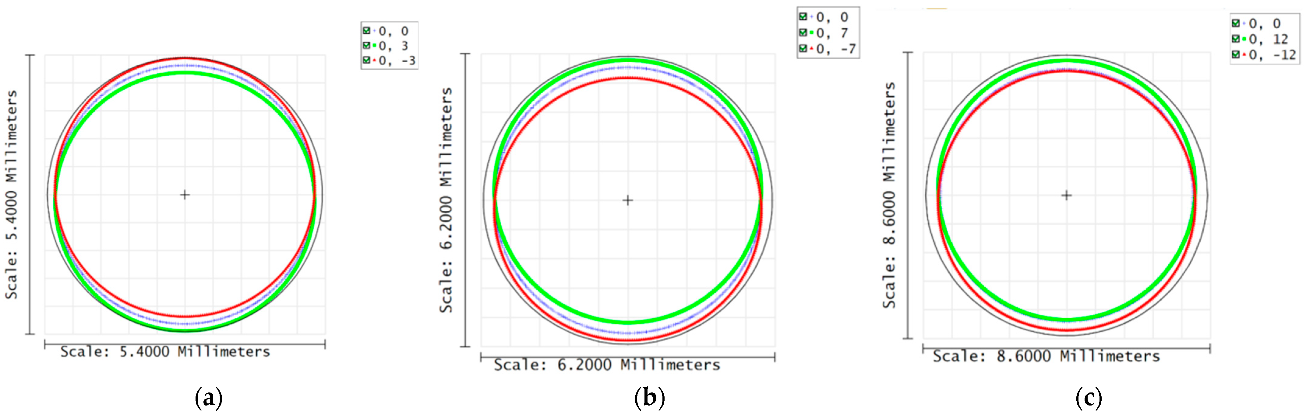
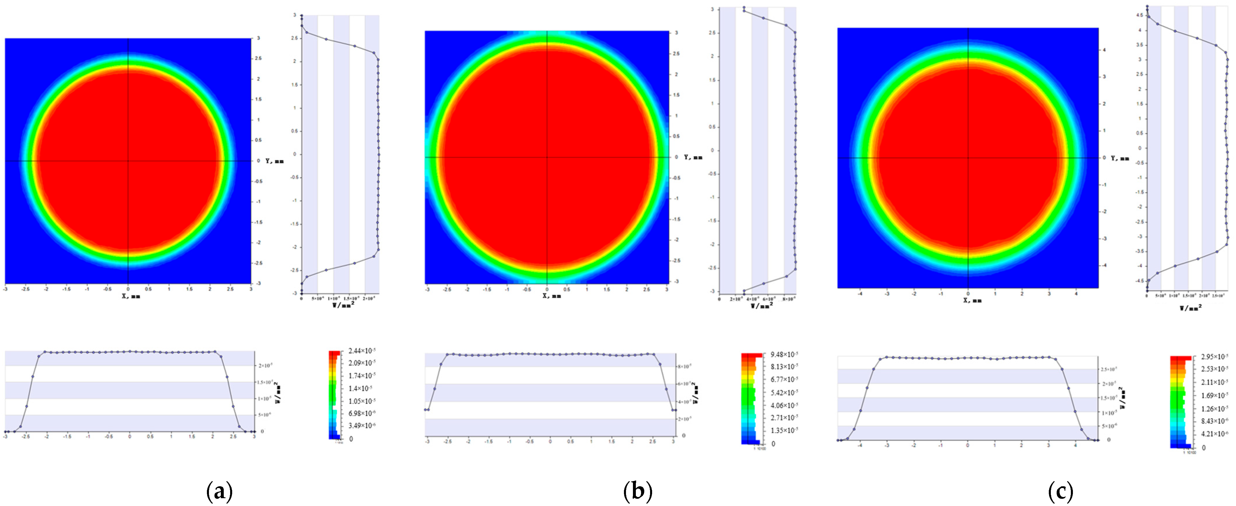
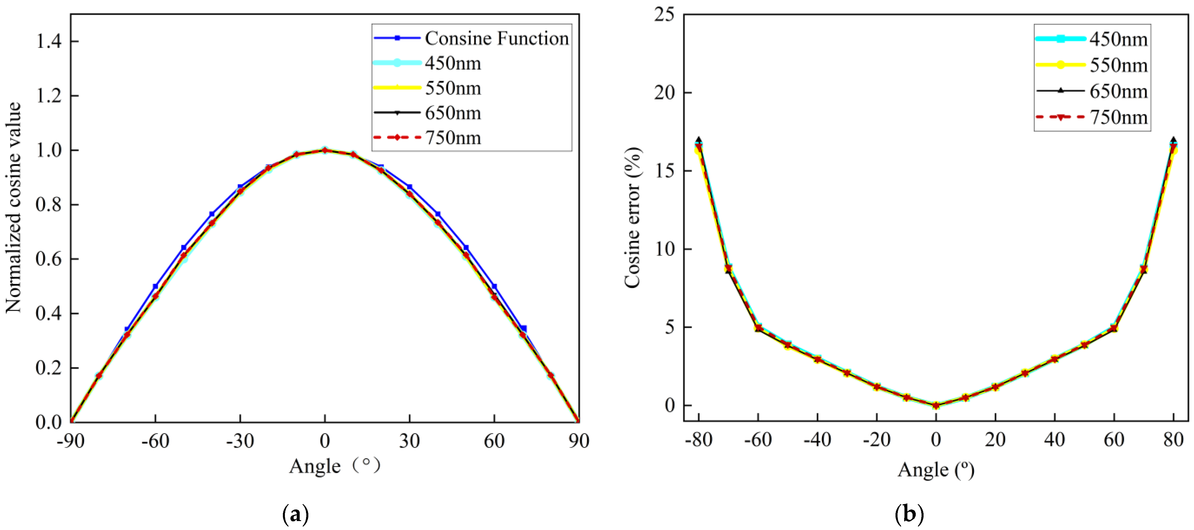
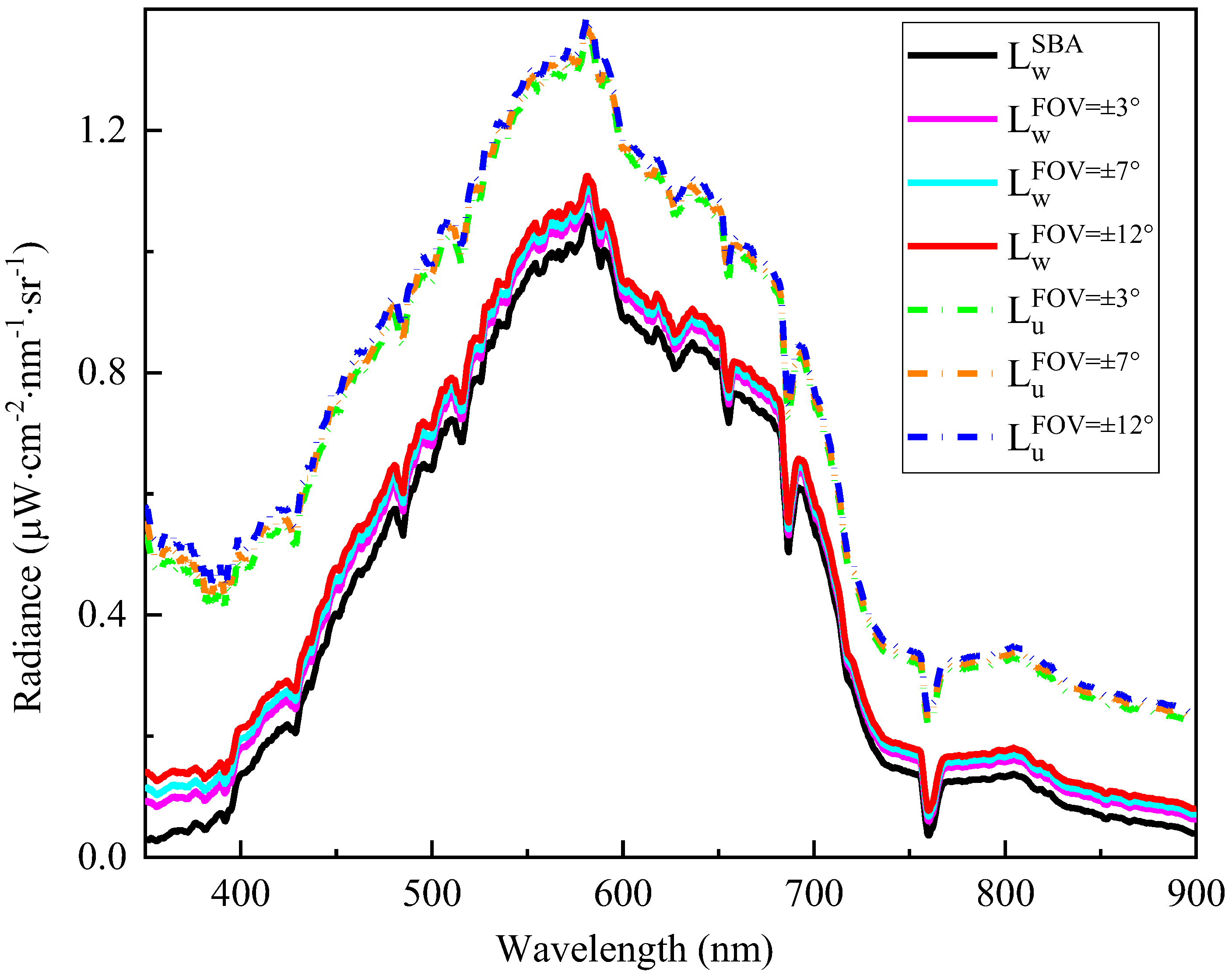
4.6. Results of GRE for Polarized Probes with Different Fields-of-View
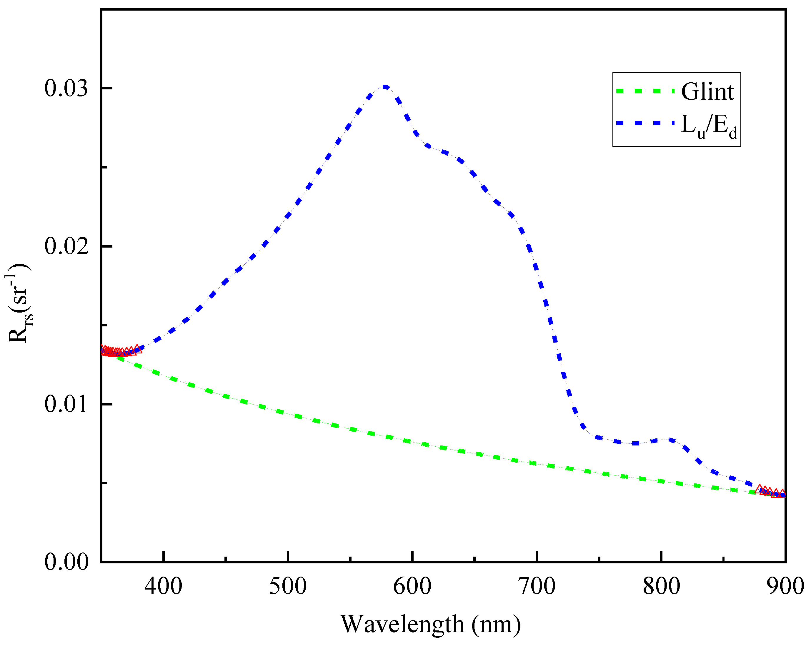
4.7. Validation of GRE Based on Dual-Band Power Function Fitting
5. Discussion
6. Conclusions
Author Contributions
Funding
Data Availability Statement
Conflicts of Interest
Abbreviations
| GRE | glint removal efficiency |
| Rrs | remote sensing reflectance |
| NIR | near-infrared |
| SBA | skylight-blocked approach |
| FOV | field-of-view |
| CV | coefficient of variation |
| UV | ultraviolet |
| SNR | signal-to-noise ratio |
| UAV | unmanned aerial vehicle |
References
- Hunter, P.D.; Tyler, A.N.; Carvalho, L.; Codd, G.A.; Maberly, S.C. Hyperspectral remote sensing of cyanobacterial pigments as indicators for cell populations and toxins in eutrophic lakes. Remote Sens. Environ. 2010, 114, 2705–2718. [Google Scholar] [CrossRef]
- Zibordi, G.; Melin, F.; Voss, K.J.; Johnson, B.C.; Franz, B.A.; Kwiatkowska, E.; Huot, J.P.; Wang, M.; Antoine, D. System vicarious calibration for ocean color climate change applications: Requirements for in situ data. Remote Sens. Environ. 2015, 159, 361–369. [Google Scholar] [CrossRef]
- Fan, C.; Warner, R.A.; Fan, C.; Warner, R.A. Characterization of Water Reflectance Spectra Variability: Implications for Hyperspectral Remote Sensing in Estuarine Waters. Mar. Sci. 2014, 4, 1–9. [Google Scholar]
- Garaba, S.P.; Voß, D.; Wollschläger, J.; Zielinski, O. Modern approaches to shipborne ocean color remote sensing. Appl. Opt. 2015, 54, 3602–3612. [Google Scholar] [CrossRef]
- Yu, X.; Lee, Z.; Shang, S.; Wang, M.; Jiang, L. Estimating the water-leaving albedo from ocean color. Remote Sens. Environ. 2022, 269, 112807. [Google Scholar] [CrossRef]
- Liu, Y.; Islam, M.A.; Gao, J. Quantification of shallow water quality parameters by means of remote sensing. Prog. Phys. Geogr. Earth Environ. 2003, 27, 24–43. [Google Scholar] [CrossRef]
- Maruyama, T.; Hashimoto, I.; Murashima, K.; Takimoto, H. Evaluation of N and P mass balance in paddy rice culture along Kahokugata Lake, Japan, to assess potential lake pollution. Paddy Water Environ. 2008, 6, 355–362. [Google Scholar] [CrossRef]
- Albert, A.; Gege, P. Inversion of irradiance and remote sensing reflectance in shallow water between 400 and 800 nm for calculations of water and bottom properties. Appl. Opt. 2006, 45, 2331. [Google Scholar] [CrossRef]
- Jeba Dev, P.; Anna Geevarghese, G.; Purvaja, R.; Ramesh, R. Measurement of in-vivo spectral reflectance of bottom types: Implications for remote sensing of shallow waters. Adv. Space Res. 2022, 69, 4240–4251. [Google Scholar] [CrossRef]
- Liu, S.; Jiang, Y.; Wang, K.; Zhang, Y.; Wang, Z.; Liu, X.; Yan, S.; Ye, X. Design and Characterization of a Portable Multiprobe High-Resolution System (PMHRS) for Enhanced Inversion of Water Remote Sensing Reflectance with Surface Glint Removal. Photonics 2024, 11, 837. [Google Scholar] [CrossRef]
- Alikas, K.; Vabson, V.; Ansko, I.; Tilstone, G.H.; Casal, T. Comparison of Above-Water Seabird and TriOS Radiometers Along an Atlantic Meridional Transect. Remote Sens. 2020, 12, 1669. [Google Scholar] [CrossRef]
- Tonizzo, A.; Gilerson, A.; Harmel, T.; Ibrahim, A.; Chowdhary, J.; Gross, B.; Moshary, F.; Ahmed, S. Estimating particle composition and size distribution from polarized water-leaving radiance. Appl. Opt. 2011, 50, 5047–5058. [Google Scholar] [CrossRef]
- Wolff, L.B.; Boult, T.E. Constraining object features using a polarization reflectance model. IEEE Trans. Pattern Anal. Mach. Intell. 1991, 13, 635–657. [Google Scholar] [CrossRef]
- Mobley, C.D. Polarized reflectance and transmittance properties of windblown sea surfaces. Appl. Opt. 2015, 54, 4828–4849. [Google Scholar] [CrossRef]
- Qian; Shen; Jun-sheng; Bing; Zhang; Yan-hong; Lei; Zou; Tai-xia. Analyzing Spectral Characteristics of Water Involving In-Situ Multiangle Polarized Reflectance and Extraction of Water-Leaving Radiance. Spectrosc. Spectr. Anal. 2016, 36, 3269–3273. [Google Scholar]
- Dev, P.J.; Shanmugam, P. A new theory and its application to remove the effect of surface-reflected light in above-surface radiance data from clear and turbid waters. J. Quant. Spectrosc. Radiat. Transf. 2014, 142, 75–92. [Google Scholar] [CrossRef]
- Harmel, T.; Gilerson, A.; Tonizzo, A.; Chowdhary, J.; Weidemann, A.; Arnone, R.; Ahmed, S. Polarization impacts on the water-leaving radiance retrieval from above-water radiometric measurements. Appl. Opt. 2012, 51, 8324–8340. [Google Scholar] [CrossRef]
- Ruddick, K.G.; Voss, K.; Banks, A.C.; Boss, E.; Vendt, R. A Review of Protocols for Fiducial Reference Measurements of Downwelling Irradiance for the Validation of Satellite Remote Sensing Data over Water. Remote Sens. 2019, 11, 1742. [Google Scholar] [CrossRef]
- Sohn, M.; Barnes, B.; Howard, L.; Silver, R.; Attota, R. Koehler Illumination for High-Resolution Optical Metrology. In Proceedings of the SPIE, Santa Clara, CA, USA, 19–24 February 2006. [Google Scholar]
- Cheng, S.; Zheng, X.; Li, X.; Wei, W.; Liu, E. Development and Calibration of a System for Measuring Apparent Optical Properties of Water. Acta Opt. Sin. 2024, 44, 0601004. [Google Scholar]
- Zhang, H.; Ye, X.; Wu, D.; Wang, Y.; Yang, D.; Lin, Y.; Dong, H.; Zhou, J.; Fang, W. Instrument Overview and Radiometric Calibration Methodology of the Non-Scanning Radiometer for the Integrated Earth–Moon Radiation Observation System (IEMROS). Remote Sens. 2024, 16, 2036. [Google Scholar] [CrossRef]
- Qiu, H.; Hu, L.; Zhang, Y.; Lu, D.; Qi, J. Absolute Radiometric Calibration of Earth Radiation Measurement on FY-3B and Its Comparison With CERES/Aqua Data. IEEE Trans. Geosci. Remote Sens. 2012, 50, 4965–4974. [Google Scholar] [CrossRef]
- Ye, X.; Yi, X.; Lin, C.; Fang, W.; Wang, K.; Xia, Z.; Ji, Z.; Zheng, Y.; Sun, D.; Quan, J. Instrument Development: Chinese Radiometric Benchmark of Reflected Solar Band Based on Space Cryogenic Absolute Radiometer. Remote Sens. 2020, 12, 2856. [Google Scholar] [CrossRef]
- Jiang, Y.; Tian, J.; Fang, W.; Hu, D.; Ye, X. Freeform reflector light source used for space traceable spectral radiance calibration on the solar reflected band. Opt. Express 2023, 31, 19. [Google Scholar] [CrossRef]
- Couto, P.G.; Damasceno, J. Methods for Evaluation of Measurement Uncertainty. In Metrology; Akdogan, A., Ed.; IntechOpen: Rijeka, Croatia, 2018. [Google Scholar]
- Zibordi, G. Experimental analysis of the measurement precision of spectral water-leaving radiance in different water types: Comment. Opt. Express 2021, 29, 19214–19217. [Google Scholar] [CrossRef]
- Wei, J.; Wang, M.; Lee, Z.; Ondrusek, M.; Ladner, S. Experimental analysis of the measurement precision of spectral water-leaving radiance in different water types. Opt. Express 2021, 29, 19218–19221. [Google Scholar] [CrossRef] [PubMed]
- Mueller, J.L.; Frouin, R.; Morel, A.; Davis, C. Ocean Optics Protocols for Satellite Ocean Color Sensor Validation, Revision 4, Volume I: Introduction. In Ocean Optics Protocols; NASA Goddard Space Flight Center: Greenbelt, MD, USA, 2003; Volume 4, pp. 1–56. [Google Scholar]
- Pahlevan, N.; Schott, J.R.; Franz, B.A.; Zibordi, G.; Markham, B.; Bailey, S.; Schaaf, C.B.; Ondrusek, M.; Greb, S.; Strait, C.M. Landsat 8 Remote Sensing Reflectance (Rrs) Products: Evaluations, Intercomparisons, and Enhancements. Remote Sens. Environ. 2017, 190, 289–301. [Google Scholar] [CrossRef]
- Wei, J.; Lee, Z.; Shang, S. A system to measure the data quality of spectral remote-sensing reflectance of aquatic environments. J. Geophys. Res. Oceans 2016, 121, 3389–3405. [Google Scholar] [CrossRef]
- Bernardo, N.; Alcântara, E.; Watanabe, F.; Rodrigues, T.; Carmo, A.; Gomes, A.; Andrade, C. Glint Removal Assessment to Estimate the Remote Sensing Reflectance in Inland Waters with Widely Differing Optical Properties. Remote Sens. 2018, 10, 1655. [Google Scholar] [CrossRef]
- Kutser, T.; Vahtmäe, E.; Paavel, B.; Kauer, T. Removing glint effects from field radiometry data measured in optically complex coastal and inland waters. Remote Sens. Environ. 2013, 133, 85–89. [Google Scholar] [CrossRef]


| Parameter | Specification |
|---|---|
| Spectral Range | 350–900 nm |
| Spectral Resolution | 3 nm |
| Wavelength Accuracy | ±0.5 nm |
| Downwelling Irradiance (Ed) | FOV: 180° Cosine Error: <5% (0–60°) |
| Water-Leaving Radiance (Lw) | FOV: ±3°; ±7°; ±12° Nadir Viewing Angle: 53° |
| Signal-to-Noise Ratio (SNR) | 400 @550–900 nm 200 @Other Wavelengths |
| Uniformity of Halogen Light System | 95% |
| Radiometric Accuracy | 3% (k = 1) |
| Water Surface Glint Removal Rate | 90% |
| FOV | Lens Name | Front Surface Radius of Curvature (mm) | Back Surface Radius of Curvature (mm) | Thickness (mm) |
|---|---|---|---|---|
| ±3° | Objective Lens | 61.0 | −61.0 | 4.7 |
| Field Lens 1 | 14.7 | −33.4 | 3.0 | |
| Field Lens 2 | 13.9 | −23.2 | 3.0 | |
| ±7° | Objective Lens | 25.2 | −25.2 | 3.4 |
| Field Lens 1 | 14.2 | −18.2 | 3.0 | |
| Field Lens 2 | 11.4 | −21.8 | 3.0 | |
| ±12° | Objective Lens | 30.4 | −30.4 | 3.1 |
| Field Lens 1 | 34.6 | −19.7 | 3.0 | |
| Field Lens 2 | 18.8 | −45.5 | 3.0 |
| Uncertainty Sources | Radiance Calibration Uncertainty Value (%) | Irradiance Calibration Uncertainty Value (%) |
|---|---|---|
| Standard Lamp Spectral Irradiance Uncertainty | 1.2 | 1.2 |
| Diffuse Reflector BRDF Uncertainty | 1.0 | - |
| Distance Uncertainty | 0.4 | 0.4 |
| Wavelength Calibration Uncertainty | 0.5 | 0.5 |
| Measurement Repeatability | 0.8 | 0.6 |
| Combined Uncertainty | 1.9 | 1.5 |
| FOV | Peak Radiance at 0° Polarization State (W·m⁻2·sr⁻¹·nm⁻¹) | Peak Radiance in Non-Polarized State (W·m⁻2·sr⁻¹·nm⁻¹) | Peak Radiance via SBA (W·m⁻2·sr⁻¹·nm⁻¹) | GRE (%) |
|---|---|---|---|---|
| ±3° | 1.08 | 1.35 | 1.06 | 93.1 |
| ±7° | 1.11 | 1.37 | 1.06 | 83.9 |
| ±12° | 1.13 | 1.38 | 1.06 | 78.1 |
| FOV | Peak Radiance at 0° Polarization State (W·m⁻2·sr⁻¹·nm⁻¹) | Peak Radiance in Non-Polarized State (W·m⁻2·sr⁻¹·nm⁻¹) | Peak Glint Radiance Derived from Power-law Fitting (W·m⁻2·sr⁻¹·nm⁻¹) | GRE (%) |
|---|---|---|---|---|
| ±3° | 1.08 | 1.35 | 0.284 | 95.1 |
| ±7° | 1.11 | 1.37 | 0.296 | 87.8 |
| ±12° | 1.13 | 1.38 | 0.310 | 80.6 |
Disclaimer/Publisher’s Note: The statements, opinions and data contained in all publications are solely those of the individual author(s) and contributor(s) and not of MDPI and/or the editor(s). MDPI and/or the editor(s) disclaim responsibility for any injury to people or property resulting from any ideas, methods, instructions or products referred to in the content. |
© 2025 by the authors. Licensee MDPI, Basel, Switzerland. This article is an open access article distributed under the terms and conditions of the Creative Commons Attribution (CC BY) license (https://creativecommons.org/licenses/by/4.0/).
Share and Cite
Liu, S.; Lin, Y.; Jiang, Y.; Cao, Y.; Zhou, J.; Dong, H.; Liu, X.; Wang, Z.; Ye, X. Kohler-Polarization Sensor for Glint Removal in Water-Leaving Radiance Measurement. Remote Sens. 2025, 17, 1977. https://doi.org/10.3390/rs17121977
Liu S, Lin Y, Jiang Y, Cao Y, Zhou J, Dong H, Liu X, Wang Z, Ye X. Kohler-Polarization Sensor for Glint Removal in Water-Leaving Radiance Measurement. Remote Sensing. 2025; 17(12):1977. https://doi.org/10.3390/rs17121977
Chicago/Turabian StyleLiu, Shuangkui, Yuchen Lin, Ye Jiang, Yuan Cao, Jun Zhou, Hang Dong, Xu Liu, Zhe Wang, and Xin Ye. 2025. "Kohler-Polarization Sensor for Glint Removal in Water-Leaving Radiance Measurement" Remote Sensing 17, no. 12: 1977. https://doi.org/10.3390/rs17121977
APA StyleLiu, S., Lin, Y., Jiang, Y., Cao, Y., Zhou, J., Dong, H., Liu, X., Wang, Z., & Ye, X. (2025). Kohler-Polarization Sensor for Glint Removal in Water-Leaving Radiance Measurement. Remote Sensing, 17(12), 1977. https://doi.org/10.3390/rs17121977