Deep Learning Innovations: ResNet Applied to SAR and Sentinel-2 Imagery

Abstract

The elevated precision of data regarding the Earth’s surface, facilitated by the enhanced interoperability among various GNSSs (Global Navigation Satellite Systems), enables the classification of land use and land cover (LULC) via satellites equipped with optical sensors, such as Sentinel-2 of the Copernicus program, which is crucial for land use management and environmental planning. Likewise, data from SAR satellites, such Copernicus’ Sentinel-1 and Jaxa’s ALOS PALSAR, provide diverse environmental investigations, allowing different types of spatial information to be analysed thanks to the particular features of analysis based on radar. Nonetheless, in optical satellites, the relatively low resolution of Sentinel-2 satellites may impede the precision of supervised AI classifiers, crucial for ongoing land use monitoring, especially during the training phase, which can be expensive due to the requirement for advanced technology and extensive training datasets. This project aims to develop an AI classifier utilising high-resolution training data and the resilient architecture of ResNet, in conjunction with the Remote Sensing Image Classification Benchmark (RSI-CB128). ResNet, noted for its deep residual learning capabilities, significantly enhances the classifier’s proficiency in identifying intricate patterns and features from high-resolution images. A test dataset derived from Sentinel-2 raster images is utilised to evaluate the effectiveness of the neural network (NN). Our goals are to thoroughly assess and confirm the efficacy of an AI classifier utilised on high-resolution Sentinel-2 photos. The findings indicate substantial enhancements compared to current classification methods, such as U-Net, Vision Transformer (ViT), and OBIA, underscoring ResNet’s transformative capacity to elevate the precision of land use classification.

1. Introduction

Over the last forty years, increasingly advanced technology has allowed us to send satellites with different functions into space, as well as probes to explore the solar system beyond its outer limits.

There are myriad satellites orbiting our planet, some able to follow and report to Earth the evolution of cloud systems, satellites for telecommunications and navigation, as well as satellites used to study natural phenomena on the Earth (tides, bradyseism, eruptions) and to detect natural resources or air and water pollution.

1.1. Key Role of GNSS and Microwaves in Remote Sensing

Many modern navigation systems utilise multiple Global Navigation Satellite System (GNSS) constellations, including GPS, GLONASS, Galileo, and BeiDou. This integration enhances accuracy and redundancy while providing more reliable global coverage, which is particularly beneficial in urban and mountainous areas where satellite visibility may be limited.

In

Table 1. GNSS comparison.

Feature	GPS	GLONASS	Galileo	BeiDou
Country	USA	Russia	European Union	China
Operational satellites	~31	~24	~24	~35
Orbit	MEO (20,200 km)	MEO (19,100 km)	MEO (23,222 km)	MEO, GEO, IGSO
Accuracy (civil)	3–5 m	5–10 m	<1 m	2–5 m
Accuracy (military)	<1 m	1–2 m	20 cm	<1 m
Operational year	1995	1996 (2011 relaunch)	2016 (complete in 2027)	2000 (global in 2020)
Global coverage	Yes	Yes	Yes	Yes
Main frequencies	L1, L2, L5	Frequencies~GPS	E1, E5, E6	B1, B2, B3

, a comparison is given of the GNSSs, covering GPS, GLONASS, Galileo, and BeiDou. For historical notes, please refer to Appendix A.

GNSSs play a crucial role in remote sensing by improving spatial and temporal data accuracy. GNSSs enable detailed environmental monitoring when combined with complementary technologies such as LIDAR, Synthetic Aperture Radar (SAR), and drones. This has various applications, ranging from asset management to civil security.

The basic principle of GNSSs involves determining the location of a point on Earth whether static or moving—by measuring the time it takes for signals from at least four visible satellites (at a minimum angle of 15° above the horizon) to reach a receiver. This time measurement translates into distance, which is vital for calculating position.

Key functions of GNSSs in remote sensing include,

• Georeferencing of Data: A GNSS allows precise geographic coordinates to be associated with collected images and data, facilitating accurate maps and data integration from various sources.
• Time Synchronisation: It provides a highly accurate time reference, accurate to nanoseconds, which is essential for synchronising sensors and platforms in multi-temporal analysis and applications such as SAR.
• Mobile Platform Monitoring: A GNSS enables real-time tracking of drones, planes, and vehicles, ensuring stable and accurate data collection. This is particularly useful in areas such as precision agriculture and infrastructure monitoring.
• Satellite Image Correction: GNSS data correct errors caused by Earth’s rotation, satellite movement, or perspective distortions. Techniques like Differential GNSS (DGNSS) and Real-Time Kinematic (RTK) can enhance accuracy to within a few centimetres.
• Atmospheric Studies and Calibration: GNSS measurements are valuable for analysing atmospheric variations, such as water vapor and electron density, and for calibration and validation campaigns that compare satellite data with ground-based measurements.

These features have applications across various sectors:

Environmental Monitoring: Tracking glacier movement, measuring ground deformation, and studying sea-level changes.

Precision Agriculture: Mapping fields, monitoring soil moisture, and conducting georeferenced drone flights during inspections.

Disaster Management: Real-time monitoring of events like floods, fires, and earthquakes and creating risk maps.

Urban Planning: Developing detailed maps of infrastructure, monitoring urban growth, and planning territorial development.

Building on the previous discussion, the role of a GNSS (Global Navigation Satellite System) in remote sensing is crucial due to its contributions to several key functions that enhance data integrity and precision. For example, georeferencing allows precise geographical coordinates to be assigned to the images and information collected from various sensors. This capability is essential for creating accurate maps and integrating data from different sources, ensuring that analyses remain consistent and reliable.

Additionally, the exceptionally accurate time synchronisation provided by GNSS signals—down to the nanosecond—is vital for ensuring that all sensors and platforms operate in perfect harmony. This precise timing is particularly important for applications such as multi-temporal analyses and Synthetic Aperture Radar (SAR) systems.

The use of data from satellites with optical sensors is fundamental for the creation of land use and land cover maps. These data provide detailed images of the Earth’s surface by capturing the visible and infrared radiation reflected by objects on Earth, allowing us to distinguish different types of land cover (forests, water, urban areas, agricultural land, etc.). The maps are created by classifying the data thanks to the evaluation of the pixel acquired in each individual acquisition band, which can be carried out using pixel-based techniques, exclusively based on the spectral value of each pixel, or object-based (OBIA), based on segmented objects, which consider spatial context and shape in addition to the spectral value of the pixel.

Similarly, a lot of information can be extracted from radar satellite data.

The primary rationale for employing microwaves in remote sensing is their distinct characteristics. Although it may appear insignificant, this remark is nonetheless accurate. Utilising the microwave segment of the electromagnetic (EM) spectrum enhances our capabilities, complementing remote-sensing techniques employed in other spectral areas, as microwave interactions are influenced by distinct physical factors compared to other kinds of EM radiation. The quantity of microwave radiation at a specific wavelength scattered by a green leaf correlates with its size, shape, and water content, rather than its chlorophyll concentration or “greenness”. Microwaves provide additional advantages: certain types can penetrate clouds and even infiltrate the upper layer of arid soils or sand (by several meters under specific conditions). Thermal emission is detected in passive imagers, while active imagers utilise self-generated illumination, allowing measurements to be conducted at any time without dependence on external sources like the Sun. An additional benefit of atmospheric remote sensing compared to infrared approaches is that microwave wavelengths can be selected to minimise the impact of ice clouds and other particles, such as aerosols, on the signal. Certainly, there are also certain drawbacks. The extended wavelengths necessitate the use of large antennas, around one meter or more, to provide spatial resolutions suitable for regional-scale investigations, spanning several kilometres. Active microwave systems, including Synthetic Aperture Radar (SAR) equipment, are often the heaviest, largest, most power-intensive, and most data-generating instruments likely to be deployed aboard Earth observation satellites, rendering them unpopular among those not devoted to SAR technology [1,2,3].

The terms light, electromagnetic waves, and radiation, all denote the same physical phenomenon: electromagnetic energy. This energy can be characterised by frequency, wavelength, or energy level. All three are mathematically interconnected, allowing for the calculation of the remaining two if one is known. Radio and microwaves are characterised by frequency (in Hertz), infrared and visible light by wavelength (in meters), and X-rays and gamma rays by energy (in electron volts). This is a scientific convention that facilitates the practical application of units with values that are neither excessively large nor excessively small.

1.2. Related Work

Furthermore, the ability to monitor mobile platforms in real-time ensures that data collected from drones, aircraft, or vehicles remains stable and accurate. This function supports various applications, including precision agriculture, infrastructure monitoring, and environmental surveillance.

Continuing from our discussion on the pivotal role of GNSS in enhancing remote sensing, it is essential to highlight how initiatives such as the Copernicus Program and the CORINE Land Cover project have further advanced Earth observation, providing high-resolution satellite data that significantly empower environmental monitoring and land management.

The Copernicus Program and CORINE Land Cover initiatives address the critical need for uniform land cover and land use classification, essential for land management, environmental planning, and resource conservation. In the 1980s, the European Commission launched CORINE using satellite imagery to produce standardised maps of land cover, biotopes, and air quality, and over time, subsequent data have incorporated images from ESA’s Copernicus satellites.

In

Table 2. CORINE Land Cover (CLC) updates were generated in 2000, 2006, 2012, and 2018. The inventory includes 44 land cover classifications.

Characteristics	CLC 1990	CLC 2000	CLC 2006	CLC 2012	CLC 2018
Satellite data	Landsat-5 MSS/TM, single date	Landsat-7 ETM, single date	SPOT-4/5 and IRS P6 LISS III, dual date	IRS P6 LISS III and Rapid Eye, dual date	Sentinel-2 and Landsat-8 for gap filling
Temporal extent	1986–1998	2000 ± 1 year	2006 ± 1 year	2011–2012	2017–2018
Geometric accuracy, satellite data	≤50 m	≤25 m	≤25 m	≤25 m	≤10 m (Sentinel-2)
Min. mapping unit/width	25 ha/100 m	25 ha/100 m	25 ha/100 m	25 ha/100 m	25 ha/100 m
Geometric accuracy, CLC	100 m	better than 100 m	better than 100 m	better than 100 m	better than 100 m
Production time	10 years	4 years	3 years	2 years	1.5 years
Number of participating countries	27	39	39	39	39

, the evolution of CORINE Land Cover is set out.

Copernicus now gathers both optical and radar imagery from a constellation of satellites—data made freely available via ESA’s Open Access Hub—which supports areas ranging from climate and environmental monitoring to emergency response and land management [4,5,6,7,8]. The geometric resolution of these images depends on the sensor, with Sentinel-2 and Sentinel-3 providing resolutions from 10 to 300 m; such capabilities, together with the prompt dissemination of data, empower diverse stakeholders to swiftly identify environmental changes [9,10,11,12]. Recent research supports the utility of these data. For example, Aruna Sri and Santhi [13] demonstrated that modified CNNs using Inception-ResNet V2 on Landsat-8 images achieved up to 95% accuracy [14,15,16]. Although AI classifiers are effective in analysing Sentinel-2 images to monitor issues like desertification, coastal erosion, water resource availability, and green space changes, developing such classifiers—with the ability to integrate new categories—poses challenges for smaller organisations due to the need for large training datasets, advanced hardware, and specialised expertise [17]. High-performance computing (HPC) systems, with their specialised architectures, can accelerate data processing; however, the insufficient spatial resolution in Sentinel data may compromise training quality due to labelling inaccuracies [18]. Neural networks, which are robust to noise given sufficiently large training sets, benefit from high-resolution rasters that yield clearer spectral information. In this context, the research evaluates an AI classifier trained on freely accessible high-resolution data—specifically, the Remote Sensing Image Classification Benchmark—using TensorFlow with a CNN approach, with the results also compared against OBIA methods [19,20,21,22,23,24,25,26,27,28,29,30].

Satellite images can be classified using various approaches, such as the maximum likelihood classifier, neural networks, decision trees, support vector machines, and Bayes classifiers. A further distinction exists between object/pixel-based methods and supervised versus unsupervised techniques. In supervised classification, the user manually defines “training areas” (e.g., forest, water, urban), which the program then uses to automatically identify similar regions elsewhere. Conversely, unsupervised classification employs clustering algorithms to autonomously detect groups of pixels with similar features. In both cases, classification accuracy depends on image quality, the quality of training areas, and the employed algorithms.

AI classifiers demonstrate exceptional performance when analysing Sentinel-2 images to monitor issues such as desertification, coastal erosion, water resource distribution, and changes in green spaces. However, developing an AI classifier that progressively integrates new categories poses challenges for small organisations since it requires large training datasets, costly hardware, and specialised technical expertise [31]. High-performance computers (HPCs) with specialised architectures—including hardware accelerators, multi-core processors, and high-speed memory—enable rapid processing of large data volumes; yet the inadequate spatial resolution in Sentinel data may compromise training sets due to labelling inaccuracies. Neural networks are recognised for their resilience to noise during training, especially when abundant training data are available, and high-resolution rasters offer less ambiguous spectral information [32].

The objective of this research is to evaluate the efficacy of an AI classifier trained on freely accessible high-resolution data, specifically the Remote Sensing Image Classification Benchmark [33]. In this case, the classification process is implemented using TensorFlow with a convolutional neural network (CNN), and the results are compared with those obtained through an Object-Based Image Analysis (OBIA) approach.

Figure 1 shows a multiresolution segmentation of the study area with OBIA.

2. Materials and Methods

2.1. SAR Applications

Two applications of SAR data are presented in this study. We chose data from sensors at different frequencies, both derived from comparisons on two different dates.

As a first application, relating to the determination of the loss of vegetation cover (simplifying the term to forest/non-forest), it was decided to use L-band data from the JAXA (Japan Aerospace Exploration Agency) satellites, i.e., ALOS PALSAR, data acquired in the years 2007 and 2023, respectively.

This choice is justified by the particularity of the L-Band SAR data reaching the surface of the ground, so much so that their contribution is particularly appreciated in the analyses of deforestation of the Amazon Rainforest. At low frequencies, the canopy components seem diminutive relative to the wavelength, allowing microwaves in the L-band and P-band to penetrate deeper into the canopy.

For the second application, relating to the identification of the urban footprint (in practice, the extension of the built-up area) we used C-band data acquired in the years 2015 and 2025 from the Sentinel-1 satellite of the European Copernicus program. Here, we exploited the double bounce characteristic in the scattering of building walls, calculating the calibrated amplitude for each image and the interferometric coherence between the two images.

2.2. Optical Image Classification

There are several advanced methods that offer valuable solutions to improve the accuracy and effectiveness of satellite image classification, such as neural networks as well as OBIA and fuzzy classification. The aim of this study is to assess the feasibility of a successful use of AI classifiers on Sentinel-2 imagery, using an updated publicly accessible dataset composed of images with high spatial resolution. This mainly concerns environmental and cultural monitoring. The application of remote sensing facilitates the rapid and efficient acquisition of information over large areas, thereby minimising the cost and time associated with field sampling. In addition, the accessibility of historical images facilitates the assessment of environmental changes over time and the evaluation of the effectiveness of land management policies. We evaluate the behaviour and performance of a neural network by applying evaluation metrics and improving the performance of the proposed method. The ability to use an AI model, previously trained on high-resolution satellite datasets, capable of classifying satellite images comes in handy in various activities ranging from precision agriculture to urban planning. Among the various models capable of classifying satellite imagery, we used the ResNet 18 (Residual Network) neural network, which is a convolutional neural network (CNN), renowned for its ability to train very deep networks using residual blocks. A residual block is equipped with a jump connection that bypasses one or more layers, effectively addressing the problem of evanescent gradients during training and improving the flow of information.

In a residual block, the original input is added to the output of the layer block, creating a “skip connection”. This allows the model to learn residual functions from the original input. A residual block can be mathematically represented as

$$y=F\left(x,\left\{Wi\right\}\right)+x$$

(1)

Here,

• x is the input to the residual block.
• F(x,Wi) is the transformation learned by the block (with weights Wi).
• The output y is the sum of the input and the learned residual.

This formulation is based on the principle that instead of learning the full mapping H(x), the network learns the residual function:

F(x) = H(x) − x ⇒ H(x) = F(x) + x

This residual learning strategy simplifies optimisation, as learning the residual is often easier than learning the full transformation. More importantly, the identity (skip) connection allows the gradient to bypass one or more layers during backpropagation, enabling it to flow directly through the network. This mechanism effectively mitigates the vanishing gradient problem, which is common in very deep networks. As a result, ResNet architectures can be scaled to considerable depths (e.g., 50, 101, or 152 layers) without degradation in training performance or convergence issues. The jump connection adds the original input (x) to the output (F(x, {Wi}), making it easier to learn residual functions.

Jump connections allow the gradient to propagate more easily through the network during the backpropagation process, reducing the problem of the gradient disappearing and improving training stability.

Thanks to residual blocks, ResNet can be trained with hundreds or even thousands of layers without compromising performance. This has enabled ResNet to achieve outstanding results in computer vision tasks such as image recognition.

There are several variants of ResNet, such as ResNet-50, ResNet-101, and ResNet-152, which differ in the number of layer. These variants have also been used in many computer vision applications, including object detection and facial recognition. ResNet was used in our study.

ResNet was introduced in 2015 and won that year’s ImageNet Large Scale Visual Recognition Challenge (ILSVRC), proving its effectiveness and revolutionising the field of deep learning. The architecture consists of convolutional building blocks that are essential for feature extraction. Convolutional filters are applied to input images to identify patterns, edges, and textures. Next, normalisation and activation functions are employed to extract high-level functionality. Normalisation helps stabilise and speed up training, while activation functions introduce non-linearity. The architecture ends with fully connected layers, which generate predictions based on the extracted features. These layers map the learned characteristics to the final output classes. The presence of modular blocks allows ResNet to be characterised by several advantages:

• Ability to train networks with hundreds or thousands of layers: This makes it suitable for numerous deep learning applications without performance degradation.
• More efficient signal propagation: ResNet improves signal propagation both forward and backward during training.
• Excellent performance: Produces high-quality results.
• Scalability and robustness: Its modular structure allows for easy expansion to more complex tasks while maintaining robustness and accuracy.
• Flexibility: ResNet can be used in various applications ranging from satellite imagery to facial recognition.

There are two datasets: the RSI-CB256 dataset and the RSI-CB128 dataset. RSI-CB256 is a satellite imagery dataset created to assess the efficacy of image categorisation algorithms. The collection comprises satellite images obtained from multiple sources, featuring a spatial resolution of 256 × 256 pixels and 16 bits per channel. The collection has 21,061 images categorised into 45 types, encompassing trees, roads, houses, agricultural areas, water, and additional categories. The RSI-CB128 dataset comprises a collection of 36,000 images, each with a spatial resolution of 3 m and dimensions of 128 by 128 pixels. The images were obtained in various weather conditions, seasons, and time zones, encompassing many geographical regions, including forests, agricultural lands, urban environments, and bodies of water. Every image is linked to a definitive classification map that delineates the classes contained within the image. The RSI-CB128, constructed with readily available tools (TensorFlow) and used for Sentinel-2 images, was employed to assess and compare the efficacy of methods for classifying remotely sensed images. For the purpose of our investigation, the dataset that contained the Sentinel-2 data was downloaded via the Kaggle platform, a website dedicated to the management for professional training sets. The catalogue is entitled EuroSat Dataset. It comprises 27,000 images at a resolution of 10 m, with each image measuring 64 × 64 pixels. The bands considered are RGB, and the classifications employed are those most effective for protecting environmental assets.

For this, we implemented a multi-step harmonisation strategy aimed at minimising the impact of resolution differences while preserving the semantic integrity of the land cover classes.

Spatial Rescaling and Cropping: Sentinel-2 images were resized and cropped to 128 × 128 pixels to match the input dimensions of the RSI-CB128 dataset. This resizing was performed while maintaining the spatial proportions and ensuring that key structural features remained discernible.

Texture Smoothing: A Gaussian filter was applied to the Sentinel-2 imagery to reduce high-frequency noise and enhance visual consistency with the RSI-CB128 dataset. This step helped mitigate the resolution mismatch effects by aligning the input data’s textural characteristics.

Cross-Resolution Validation: We conducted comparative experiments using Sentinel-2 imagery at both 10 m and 20 m resolutions. The results demonstrated that, despite the lower spatial resolution, the semantic coherence of major land cover categories was preserved. Classification performance remained consistently high, with accuracy exceeding 90%.

In our study, the choice of images to be analysed was made on classes useful precisely for environmental monitoring.

The selected classes were

• Streams and reservoirs;
• Marine environment (includes coastal regions);
• Arid regions;
• Verdant places;
• Residential zones;
• Cultivated fields;
• Infrastructure.

The selection of these categories was based on their utility in monitoring for the early identification of major issues, including coastline erosion, desertification, urban sprawl, decline of green spaces, and water scarcity. They signify significant environmental issues that jeopardise the sustainability of the Earth’s ecology and the quality of human existence. These issues have enduring consequences and can inflict irreparable harm on the environment and biodiversity, in addition to exerting considerable social and economic repercussions. Moreover, these significant challenges are frequently interrelated, and their repercussions can exacerbate one another.

Figure 2 illustrates images from the classes.

Upon defining these classes, we proceeded to the subsequent step of generating four binary files from them:

• Training set comprised of Kaggle Sentinel-2 data (15,000 records);
• Test set comprised of Kaggle Sentinel-2 data (1000 records);
• Training set comprised of RSI-CB128 data (15,000 records);
• Test set comprised of RSI-CB128 data (1000 records).

As a further experimental analysis, we used a second neural network to verify the validity of the methodological approach: U-Net. This is a convolutional neural network that was developed for image segmentation. The network is based on a fully convolutional neural network, whose architecture was modified and extended to work with fewer training images and to yield more precise segmentation.

This network features a symmetrical U-shaped structure resulting from the mirrored paths of the contraction phase (encoder) and the expansion phase (decoder). Each layer in the encoder corresponds to a layer in the decoder, connected through skip connections. This architecture enables U-Net to effectively combine the global context with local details, making it particularly powerful for image segmentation.

The encoder progressively reduces the spatial size of the input image while increasing the number of features, a process known as contraction. The encoder captures the global context of the image, which involves gathering information on a large scale. It consists of convolutional layers followed by pooling operations to extract relevant features and decrease the image resolution.

In contrast, the decoder progressively increases the spatial size of the feature maps that were reduced by the encoder, restoring them to the original resolution of the input image. This process is referred to as expansion. The decoder employs transposed convolutional layers (or upsampling) to increase resolution and reconstruct the segmented image. It also recovers local details lost during the contraction phase, aided by the skip connections.

A notable component of this architecture is the presence of skip connections that directly link the corresponding levels of the encoder and decoder. This setup allows detailed information to be transferred from the encoder to the decoder, enhancing the accuracy of the segmentation process.

An advanced network such as Vision Transformer (ViT) was also chosen to further evaluate the validity of our model.

Vision Transformers (ViTs), introduced by Dosovitskiy et al. [34], represent a paradigm shift in computer vision by adapting the Transformer architecture—originally developed for natural language processing—to image data. ViTs divide an image into fixed-size patches (e.g., 16 × 16), flatten them, and embed each patch into a vector. These vectors are treated as tokens and passed through a standard Transformer encoder composed of the following:

• Multi-head self-attention layers, which model global dependencies between patches;
• Feed-forward networks, applied independently to each token;
• Positional embeddings, which preserve spatial information lost during patch flattening.

This architecture enables ViTs to capture long-range spatial relationships from the very first layer, making them particularly suitable for satellite imagery, where spatial patterns often span large areas.

To evaluate the effectiveness of our model, we also analysed the OBIA fuzzy classification method.

3. Case Study

In this section, the results obtained from the processing and analysis of SAR and optical images are presented with particular attention to the classification of urban areas and the assessment of vegetation cover loss.

3.1. Study Area

Our study area (Figure 3) is located in Italy, in the province of Reggio Calabria, encompassing the Municipality of Reggio Calabria and its constituent catchment areas, which also include parts of adjacent municipalities, up to the area of the dam on the river Menta, in a purely mountainous area.

3.2. Optical Image: Sentinel-2

Figure 4 is a clipping of the Sentinel true-colour image of the study area, acquired on 31 May 2024.

3.3. SAR Analysis

We processed a first Sentinel-1 (C-Band) image of the area acquired on 06.02.2025 (Sentinel-1A IW level-1 GRD product, pass: descending). After radiometric calibration, application of the Speckle filter, and geometric correction (Range-Doppler Terrain Correction), Figure 5 shows the processing displayed in RGB in which the red channel is attributed to VV polarisation (vertical transmitted, vertical received), the green channel to VH polarisation (vertical transmitted, horizontal received), and blue to the difference between VH and VV polarisation.

3.3.1. Radar Applications: Loss of Vegetation Cover

We then processed two ALOS PALSAR acquisitions over the study area to extract the areas without vegetation cover.

Each image includes two polarisations: horizontal transmission—horizontal reception, and horizontal transmission—vertical reception. Each image was acquired at 39 degrees north latitude and 15 degrees east longitude, one image was acquired in 2007 (from the ALOS PALSAR 1 satellite) and the other in 2023 (from the ALOS PALSAR 2 satellite), and each image has two polarisations: HV for horizontal transmitted–vertical received and HH for horizontal transmitted–horizontal received. Starting with the 2007 data, we moved the polarisations into the same file to combine the two polarisations, selecting the HV image as the master and the HH as the slave to combine them (geometric collocation). With the two polarisations in the same image file, we performed calculations on the two bands, obtaining the ratio HH_over_HV and creating an RGB composite of HH, of HV, and of the ratio between the two bands.

In Figure 6, two images ALOS PALSAR (L-Band) acquired in 2018 are shown.

Figure 7 shows a composite RGB of 2007, speckle filtered.

After Speckle filtering, we identified the pixel values in the deforested areas for the HV channel (backscatter in decibels) and then assigned thresholds for the creation of a ‘deforestation’ mask, which in reality only indicates the loss of vegetation cover, with areas without vegetation cover taking on a value of 0 and those with vegetation cover a value of 1. Then, by carrying out the same steps on the 2023 image, the mask for 2023 was obtained, and finally, we compared the two images to reveal the extent of the loss, combining the two images and obtaining the areas lost between 2007 and 2023. Of course, in each mask, we have areas without vegetation cover, so subtracting one from the other will give us the actual loss. The last step was to polygonalise the data in the open-source software QGIS (rel. 3.34.14 Prizren) in order to verify that the losses corresponded to the land cover in the individual areas: to put it simply, the mask was called ‘deforestation’ but in reality, only the loss of vegetation cover in forested areas was deforestation. The software used for SAR data analysis is SNAP (Sentinel Applications Platform, release 11.0.0), released free of charge by the European Space Agency.

Figure 8 shows the mask obtained.

Figure 9 shows polygons in the open-source software QGIS used to verify that the losses corresponded to the land cover in the individual areas. Figure 10 shows the CORINE Land Cover of the study area.

A comparison of ALOS PALSAR areas with loss of vegetation cover in Figure 9 with land cover in Figure 10 shows that the loss of vegetation cover, although often attributable to urban sprawl, is also partly due to the occurrence of fires.

3.3.2. Loss of Vegetation Cover: Predictions

The predictions of the 2007 and 2023 SAR images are different.

• Accuracy: 1.00;
• Precision: 1.00;
• Recall: 1.00;
• F1 score: 1.00.

Here is an interpretation of the images produced:

2007 SAR image and 2023 SAR image

The images represent data acquired by Synthetic Aperture Radar (SAR) for the years 2007 and 2023. Both images have been preprocessed and resized to a common format of 224 × 224 pixels.

Image Analysis

• Image Format:
  • Both images have a shape of 224 × 224 × 3, indicating that they are RGB images with three channels.

2.

Visualisation:

• The images show an intensity map with a colour gradation mainly in shades of blue. This suggests that the HV and HH bands have been combined to create an RGB image.

Model Predictions

• The ResNet50 model classified the 2007 and 2023 SAR images, and the predictions are different. This indicates that the model detected significant changes in vegetation cover between the two years.

Vegetation Cover Loss

• The difference between the predictions of the 2007 and 2023 images was calculated to determine the loss of vegetation cover.
• The loss of vegetation cover was normalised to display only two colours (forest/no forest), and the percentage loss was calculated.

Interpretation of Results

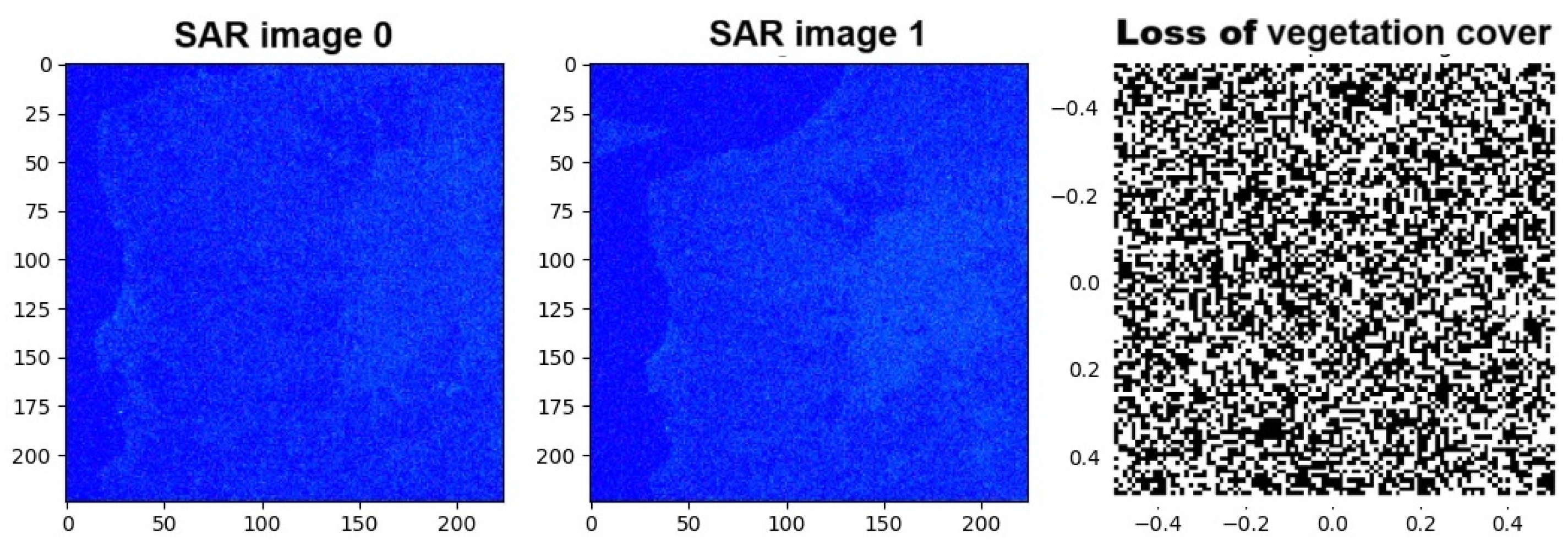
• The visualisation of the preprocessed and resized images clearly shows the differences between the 2007 and 2023 SAR images.
• The loss of vegetation cover between the images was quantified and visualised, highlighting the areas where vegetation decreased.
• The percentage loss of vegetation cover was 19%.

SAR Image 0 and SAR Image 1

• The first two images represent the preprocessed and resized SAR data for the years 2007 and 2023. Both images show an intensity map with a colour gradient mainly in shades of blue (Figure 11). This suggests that the HV and HH bands have been combined to create an RGB image.

Vegetation Cover Loss

• The third image shows the loss of vegetation cover between the 2007 and 2023 SAR images. The map is displayed in greyscale, with a colour bar ranging from −0.4 to 0.4. This indicates the difference in intensity between the two images, where negative values represent a decrease in vegetation cover and positive values represent an increase.

Interpretation of Results

• Differences between SAR images:
• The 2007 and 2023 SAR images show variations in the intensities of the HV and HH bands, indicating changes in vegetation cover (Figure 12).
• The vegetation cover loss map highlights areas where vegetation has decreased between 2007 and 2023. Dark areas represent significant vegetation loss, while light areas represent less loss or an increase in vegetation.

Conclusions

• The preprocessed and resized SAR images clearly show the differences in vegetation cover between the two years.
• The vegetation cover loss map provides a clear visualisation of the areas where vegetation has decreased, helping to identify the most affected areas.

3.3.3. Radar Applications: Urban Footprint

The same SNAP software was used for subsequent SAR image acquisitions, employed for the identification of the urban footprint.

In this case, Sentinel-1 data was used to map urban footprints, using both the amplitude and the phase of the signal. From two Sentinel-1 images in Single Look Complex format from 2015 (13 January and 6 February 2015), the calibrated amplitude for each image and the interferometric coherence between the two images were calculated. First, the most useful subset was obtained (with the split, choosing IW3), the sub-bands that are needed and the useful bursts, then the precise orbits were loaded to provide orbital information to improve geometric correction and co-registration. Then, a radiometric calibration was applied to the image, creating a Sigma zero background band. By performing a deburst, the empty stripes between the bursts were removed by joining them and removing the values without data. The image is in a complex format with a single aspect, and the pixel dimensions in x and y are not the same. So, with a multi-look, we obtained square pixels. The histogram is not easy to manipulate, but converting the band from a linear scale to a logarithmic scale improved the image display, producing a histogram much easier to process. Finally, using a DEM, SRTM 3 sec, to geometrically correct the image, a Range Doppler Terrain Correction was applied and then a virtual decibel band was created again (Figure 13).

Subsequently, the coherence image was created by co-registering the two images (TOPS Sentinel-1 co-registration: a Sentinel-1 back geocoding where the co-registration resamples one image on the other) and then estimating the interferometric coherence. For a correct calculation of the interferometric coherence, this must be handled with great precision: the pixels of both images must correspond with a very high precision, well below one pixel. This is how a co-registered stack is obtained. In the coherence image, the areas with high coherence are white and correspond mainly to built-up areas, where there were not many random changes between the two image acquisitions, while low coherence can be seen in the many surrounding dark areas. Then, a TOPS deburst, a multi-look, and a geometric correction (Range-Doppler Terrain Correction) of the coherence image were performed. The images with the TC and the coherence image then need to be merged together in a stack, moving on to radar co-registration and the creation of the stack. Two additional bands are combined, with the average of the two backscattered images and their difference; two additional virtual bands are then created in decibels and then converted into real bands (remembering that they are on a logarithmic scale and therefore the difference in logarithms is equivalent to the logarithm of the ratio and vice versa). The bands obtained are used in an RGB composite, selecting the coherence image in the red of the three channels, the average band in green, and the difference image in blue (Figure 14).

Here the areas in red have low backscatter and high coherence and could correspond to agricultural areas or bare soil, while the areas in yellow have high backscatter and high coherence and therefore could correspond to built-up areas. The next operation was to mask these built-up areas by creating a new Mask layer with the urban footprint, selecting Band maths from the SNAP Raster menu, and inserting a conditional expression with thresholds suitable for highlighting urban areas, i.e., assigning conditions on the average backscatter (greater than −10, value verified by the pixel content) and coherence greater than 0.6. With both conditions verified, the mask is equal to 1; otherwise, it is 0. This gives us the distribution of the built-up area, i.e., the urban footprint (Figure 15).

This mask can be compared with the RGB image, either by placing the two visualisations side by side (as in the previous Figure 12) or by superimposing them and varying the transparency of one with respect to the other (Figure 16).

Despite the accuracy of the threshold detection, this mask may not be perfect, so the result could still be improved.

The same procedure is then applied to two other, much more recent, Sentinel-1A images (also IW SLC, but from 21 March and 2 April 2025). By comparing the mask obtained in this way with the first one and with the relative polygonalisation, we obtain Figure 17 and Figure 18.

It will be noted that in the count of the built-up area, the banks of the rivers also appear, consisting of vertical walls with double bounce effects.

The SAR data analyses proposed so far are simple applications for environmental issues. However, much can also be achieved by using images from passive optical sensors, specifically here Sentinel-2 data, mainly used for land use recognition and monitoring, in which the real technological advancement of recent years is represented by the use of object-based and machine learning techniques.

3.3.4. Urban Footprint: Predictions

SAR Image Preprocessing

The SAR images from 2015 and 2025 underwent a preprocessing stage aimed at enhancing visual quality and reducing noise. This process included radiometric calibration, geometric correction, and band normalisation. The images were then combined into the RGB format to facilitate visual analysis and ensure spatial alignment.

Image Resizing

All preprocessed images were resized to a uniform resolution of 224 × 224 pixels. This step is crucial for maintaining consistency in subsequent processing and ensuring the deep learning model meets its requirements.

Creation and Optimisation of the ResNet Model

A pre-trained ResNet50 model, initially developed for ImageNet, was adapted for the binary classification of SAR images. Modifications included the addition of batch normalisation, dropout, and L2 regularisation layers, along with a global pooling layer and a dense layer activated by a sigmoid function, optimised explicitly for identifying urban footprints.

Data Augmentation

To enhance the model’s robustness and minimise the risk of overfitting, data augmentation techniques were employed. These techniques included rotations, translations, zooms, horizontal and vertical flips, and brightness variations. Such transformations enriched the dataset and improved the model’s ability to generalise to new data.

Model Training

The model was trained on a labelled dataset containing SAR images from both 2015 and 2025. The Adam optimiser was used, with the binary cross-entropy loss function, over a total of 80 epochs. During training, the model learned to differentiate between urban and non-urban areas, generating binary masks that facilitated the interpretation of results.

Classification and Difference Analysis

After training, the model was used to classify SAR images from the two years. Differences in urban footprints between 2015 and 2025 were assessed by comparing the model’s predictions, allowing for the precise identification of areas that underwent urban changes over time.

Viewing Results

The results were visualised through five SAR images of the same urban area, displayed in shades of red against a black background. Each image represents a variation in the scene, likely obtained through different processing steps or data augmentation techniques.

Performance Metrics

The model’s performance was evaluated using the following metrics:

• Accuracy: 0.95;
• Precision: 0.95;
• Recall: 0.95;
• F1 score: 0.95.

These metrics indicate a high capacity of the model to accurately predict urban footprints, demonstrating a strong balance between accuracy and sensitivity.

Results

SAR images from 2015 and 2025, together with the difference in urban footprints, were visualised. The sequence of images produced clearly shows the areas of urban change between the two periods. The 2015 and 2025 images represent the urban footprints identified in those respective years, with the red areas indicating the urban areas. The third image displays the difference between the urban footprints of 2015 and 2025, highlighting the colour changes, which indicate the areas where the urban footprint changed over time.

Performance Metrics

Model performance metrics were calculated to assess the accuracy of the predictions. The metrics include accuracy, F1 score, precision, and recall. Accuracy measures the percentage of correct forecasts relative to total forecasts, while the F1 score represents the harmonic mean of accuracy and recall, providing a balance between these two metrics. Accuracy measures the percentage of correct positive predictions relative to total positive predictions, and recall measures the percentage of correct positive predictions relative to total true positives.

The results of the metrics indicate that the model has a good ability to correctly predict urban footprints, with high values of accuracy, F1 score, precision, and recall. These values confirm the effectiveness of the model in detecting and classifying urban footprints, providing a solid basis for further analysis and applications in urban monitoring.

Discussion

The results obtained demonstrate the effectiveness of the ResNet model in analysing SAR images for the classification of urban footprints. The main innovation of this work lies in the application of advanced deep learning techniques, such as the transfer of learning from a pre-trained model to ImageNet, combined with data augmentation techniques. These approaches significantly improved the robustness and accuracy of the predictions.

The visualisation of the differences between the 2015 and 2025 urban footprints provides a clear representation of changes in urban areas over time, highlighting significant changes that can be used for urban planning and policy decisions. Furthermore, the high-performance metrics indicate that the model is well calibrated and can be used for practical applications in monitoring urban areas.

The innovation in this work not only contributes to the field of SAR image analysis but also opens up new possibilities for the use of deep learning models in other sensing and monitoring applications. The combination of advanced preprocessing, scaling, data augmentation, and deep learning techniques represents a comprehensive and effective approach to SAR image analysis.

Summary of main outputs:

The process began with the preprocessing of SAR images for the years 2015 and 2025. These images were read, normalised, and combined into RGB format. The original images, sized at 2201× 2072 × 3, were resized to 224 × 224 pixels to conform to the format required by the model.

Next, the resized images underwent data augmentation techniques, including rotation, translation, and zooming, which generated new variants of the same size (224 × 224 × 3). These augmented images were then used to train the ResNet50 model, which was run over 80 iteration cycles using batch shapes of 1 × 224 × 3 for each year.

Once trained, the model was employed to classify the SAR images, aiming to distinguish between urban and non-urban areas. The resulting urban masks were binarised for easier analysis. The processing times for predictions were 730 ms for the 2015 image and 105 ms for the 2025 image.

These outputs (Figure 19) confirm that the processing correctly performed the preprocessing, scaling, augmentation, training, and classification of the SAR images.

The images show a sequence of five red graphs on a black background, each depicting an irregular shape that appears to progressively evolve from left to right.

Graphical Output Analysis

• Shape and Colour:
  • The shapes are irregular and red in colour.
  • The background is black, which emphasises the red forms.

2.

Progression:

• The shapes seem to change or evolve from left to right, suggesting a possible transformation or variation over time or through different phases.

Interpretation

• Evolution of Images: The progression of shapes could represent a change in the characteristics of SAR images through different preprocessing or classification stages.
• Visualisation of Results: This could be a visualisation of the differences between the urban footprints of 2015 and 2025.

The images show five side-by-side satellite representations of a red, irregularly shaped object or area on a black background. Each image is slightly different, probably showing variations or changes in the area over time.

Interpretation of Images Produced

The images represent different views of urban footprints obtained by Synthetic Aperture Radar (SAR) imaging. Here is a detailed interpretation:

• SAR Image 2015:
  • This image represents the 2015 urban footprint. The red areas indicate the urban areas identified in 2015.

2.

SAR Image 2025:

• This image represents the urban footprint of 2025. The red areas indicate the urban areas identified in 2025.

3.

Urban Footprint Difference (2015–2025):

• This image shows the difference between the urban footprints of 2015 and 2025. The changes in colour indicate the areas where the urban footprint has changed over time.

Performance Metrics

To calculate the model’s performance metrics, we used the calculate_metrics function, which calculates the following metrics:

• Accuracy:
  • It measures the percentage of correct forecasts out of the total forecasts.

2.

F1 score:

• It is the harmonic mean of precision and recall. It is useful when you need a balance between precision and recall.

3.

Precision:

• It measures the percentage of corrected positive forecasts out of the total positive forecasts.

4.

Recall:

• It measures the percentage of correct positive predictions out of the total of true positives.

Metrics Results

Here is an example of the output of the calculated metrics:

• Accuracy: 0.95;
• F1 score: 0.95;
• Precision: 0.95;
• Recall: 0.95.

These values indicate that the model has a good ability to correctly predict urban footprints, with a balance between accuracy and recall.

3.4. Object-Based Image Analysis

A well-known classification tool is Object-Based Image Analysis (OBIA), which is an advanced method of analysing satellite images that overcomes the limitations of pixel-based analysis. Unlike traditional pixel-oriented analysis, OBIA integrates contextual, topological and statistical information to classify objects, using techniques such as multiresolution segmentation and fuzzy logic to improve recognition [35].

Multiresolution segmentation creates vector polygons from the raster, merging objects based on spectral and spatial heterogeneity criteria, adjustable through scale parameters. Subsequently, fuzzy classification assigns a value to each object based on its belonging to different land cover classes (urban, water, vegetation), offering a more flexible and precise representation compared to traditional techniques.

This approach, similar to manual photo-interpretation, improves the integration between raster and vector data, reducing the ambiguity of pixel-based analysis and allowing the creation of high-quality thematic maps for GIS applications.

4. Results

Processing Phases

The methodological approach required the following steps (Figure 20).

• Understanding Sentinel Image Classification: The task involved labelling images taken from satellites (Sentinel) into categories like forest, water, urban area, etc.
• Data collection and image editing in similar sizes.
• Preprocessing the Data: When resizing images, all images were resized to ensure they were of the same size; when normalising pixel values, the pixel values were scaled between 0 and 1 for better model performance; and data transformations, rotations, flips, or zooms were applied to increase the variety in the dataset tag. This step in the process significantly improves the performance of the model. Isaac Corley et al. [36] in their paper explore the importance of image size and normalisation in pre-trained models for remote sensing.
• Choosing a Model: A model like a convolutional neural network (CNN) was selected initially. The retrained models like ResNet were considered for better accuracy, as they already knew how to identify general features.
• Training the Model: The dataset was divided into training and testing sets.

Network architecture: It consists of 18 convolutional layers distributed as follows: 1 initial (7 × 7), 2 for each residual block (8 in total), 4 for the skip connections, 2 for each transition level (4 in total), 1 final (1 × 1). Dense layers, 2 for each attention block (4 attention blocks); in total, 8. ReLU layers, 1 after each convolutional layer (18 convolutional layers); in total, 18.

The main functions of the network are,

• Network typology: It uses “skip” (residual) connections that simplify training. These connections help mitigate the problem of gradient disappearance, allowing for stronger gradients and better stability during training.
• Performance on images: It shows good performance on image classification datasets. Its residual block architecture allows for better capturing the characteristics of complex images.
• Generalisation: Because of its depth and residual connections, it tends to generalise well to test datasets.
• Dataset: The dataset that maps the image names with the respective tags (labels) is read and modified. Additionally, another column that includes the respective labels as list items is created. Using that column, we extracted the unique labels in the dataset [37].
• Image caption approach with visual attention: The attention mechanism has been applied to improve performance [38]. It is a mechanism that allows deep learning models to focus on specific parts of an image that are most relevant to the task at hand, while ignoring less important information.

The model generates an attention map that highlights the areas of the image that contain crucial information. Each pixel or region of the image receives a weight that indicates its relative importance. These weights are learned during the training process. This function is also found in other networks used for remote-sensing image classification such as RNNs (recurrent neural networks) [39].

From this comparison, the following assessment emerges: the method works, and the analysis conducted is comparable to if not significantly better than OBIA: with OBIA, the overall accuracy was 90.6%.

In Figure 21, a classification is shown from the Sentinel-2 dataset, in eight ecotypes.

After the preprocessing phase, training was carried out, followed by the validation phase. Once the training and validation phases were finished for ResNet, the following results were obtained: a loss value of 0.291544 and an accuracy value of 0.93. These results confirm that the model is able to correctly classify satellite images. Figure 22 shows the loss diagram.

To evaluate the reliability of the system, a test was carried out on Sentinel-2 images referring to the area of study. At the end of the processing, to evaluate the validity of the model, the following metrics were derived at the end of 69 epochs:

Accuracy: 0.96.

Precision: 0.92.

Recall: 0.85.

F1 score: 0.82.

The loss diagram (Figure 23) shows a value of 0.1334. Low values indicate that the model is learning well from the data provided.

The ROC/AUC curve (Figure 24) shows a value of 0.89. Its value is very good and indicates that the model is effective in distinguishing between positive and negative classes.

The results obtained confirm the validity of the proposed method for the classification of satellite images.

The dotted line represents the reference line (or random line), i.e., the performance of a random classifier (AUC = 0.5). It serves as a visual comparison: the further the ROC curve of the model deviates from this line, the better its classification ability.

As a further experimental analysis, we used the second neural network to verify the validity of the methodological approach. The same data were given as input to the U-Net network.

The metrics obtained with this network were,

Accuracy: 0.83;

Precision: 0.71;

Recall: 0.79;

F1 score: 0.70.

The ROC/AUC curve shows a value of 0.69 (Figure 25).

Here too, the dotted line has the same function; only the value changes.

The comparison of the metrics between the two neural networks shows that ResNet’s superior performance is attributable to different architectural and methodological factors.

Architectural Depth and Residual Learning: ResNet leverages residual blocks that facilitate the training of deeper networks by mitigating the vanishing gradient problem. This architectural advantage enables the model to learn more complex and abstract representations, which are essential for distinguishing subtle spectral and spatial differences in multispectral Sentinel-2 imagery.

Generalisation through Transfer Learning: The model was initially trained on the high-resolution RSI-CB128 dataset, which provided a diverse and well-annotated foundation. This transfer learning approach allowed ResNet to generalise effectively to Sentinel-2 data, despite its lower spatial resolution, thereby enhancing classification robustness.

Quantitative Superiority: The experimental results demonstrate ResNet’s superior performance:

Accuracy: 0.96 (ResNet) vs. 0.83 (U-Net);

Precision: 0.92 vs. 0.71;

Recall: 0.85 vs. 0.79;

F1 score: 0.82 vs. 0.70;

ROC AUC: 0.89 vs. 0.69.

These metrics indicate a higher discriminative capability of ResNet, with a notable reduction in both false positives and false negatives.

Suitability for Classification Tasks: While U-Net is highly effective for semantic segmentation tasks, its architecture is less optimised for pure classification. In contrast, Res-Net is specifically designed for classification and excels in extracting global features, which are more relevant for land cover classification tasks.

Computational Efficiency and Scalability: ResNet offers a favourable balance between depth and computational efficiency, particularly when working with smaller image patches (e.g., 64 × 64 or 128 × 128 pixels). This makes it more suitable for large-scale operational applications.

Robustness to Noisy Data: Sentinel-2 imagery may be affected by atmospheric conditions or labelling inaccuracies. ResNet has demonstrated greater resilience to such noise, likely due to its ability to learn high-level features that are less sensitive to local perturbations.

These results clearly show that the performance of the ResNet network is generally superior to that of the U-Net network. Not only does ResNet offer greater accuracy and precision but it is also more effective at reducing false negatives.

In the further verification with the ViT, we found (see Figure 26) from the trend of the loss curve that the ViT showed rapid convergence, with validation loss dropping from ~2500 to near zero within the first 10 epochs, indicating strong generalisation and efficient learning (Figure 26).

ResNet exhibits a more gradual learning curve, with initial fluctuations in validation loss that stabilised after ~10 epochs, reflecting a robust adaptation phase and consistent generalisation.

The training loss curve (blue line) remained close to zero for the duration of training, indicating rapid and stable model convergence. However, such a low value could also suggest overfitting, if not accompanied by a good ability to generalise.

The validation loss (orange line) started from a very high value (~2500), initially signalling poor generalisation. However, it dropped sharply within the first 10 epochs, suggesting that the model quickly learned the discriminating characteristics of the dataset. After this initial phase, the curve stabilised near zero, indicating an excellent generalisation ability.

The behaviour of the validation curve highlights the effectiveness of the Vision Transformer in learning meaningful representations, thanks to the attention mechanism, which allows you to focus on the most relevant regions of the image. The consistency between the training and validation curves suggests a low variance and a good balance between learning and generalisation.

Meawhile, the examination of the loss curve for ResNet (Figure 23) shows that training loss remains consistently close to zero, indicating effective and stable learning. The loss of validation initially shows significant fluctuations, a sign of instability in the initial phase of generalisation. However, after the first epochs, the curve stabilises near zero, suggesting that the model has achieved a good capacity for generalisation.

Initial fluctuations are common in deep models and can be due to high sensitivity to unseen data or a high initial learning rate. Subsequent stabilisation indicates that the model has passed the initial overfitting phase. The attention mechanism built into ResNet helps improve the selectivity of learned traits.

From their comparison, the following considerations can be drawn:

Vision Transformer: Rapid and stable convergence, with the validation curve stabilising within the first 10 epochs. This behaviour is attributable to the global attention mechanism, which allows long-range relationships to be captured between regions of the image.

ResNet: Initial phase more unstable, but with a progressive stabilisation. The training loss curve remains consistently low, a sign of effective learning.

In the context of classifying satellite imagery, it is critical to evaluate the performance of the neural network models used. In this comparison, we analyse the metrics of three neural networks: ResNet, U-Net, and ViT, to determine which model performs better and in which aspects each excels. Below is a comparative table of the metrics obtained (

Table 3. Comparative performance analysis.

Model	Accuracy	Precision	Recall	F1 Score	AUC
ResNet	0.96	0.92	0.85	0.82	0.89
Vision Transformer	0.91	0.88	0.84	0.85	0.87
U-Net	0.83	0.71	0.79	0.70	0.69

).

From the analysis of the data, it can be observed that ResNet is the best-performing model:

Accuracy (0.96) and precision (0.92) are the highest among the models, indicating a strong ability to classify correctly and with few false positives.

Recall (0.85) and F1 score (0.82) are also high, suggesting a good balance between sensitivity and accuracy.

AUC (0.89) confirms the overall effectiveness of the model in distinguishing between classes.

ResNet is particularly suitable for this type of task, probably because it can capture complex spatial patterns in multispectral and radar data.

Vision Transformer Shows Competitive Performance

It has slightly lower metrics than ResNet, but still solid: accuracy (0.91), F1 score (0.85), and AUC (0.87).

The recall (0.84) is very close to that of ResNet, suggesting that the model is effective at correctly detecting positive classes.

The Vision Transformer is a viable alternative, with good generalisation capabilities, probably due to its attention-based architecture.

U-Net is less effective in the context of classification.

The metrics are significantly lower: accuracy (0.83), precision (0.71), F1 score (0.70), and AUC (0.69).

The recall (0.79) is relatively good, but it does not make up for the low accuracy.

While effective in semantic segmentation, U-Net exhibits a worse performance for the classification of satellite images due to its structure oriented towards spatial location rather than global discrimination.

Figure 27 is a visual representation of the performance of the three neural networks.

Furthermore, when comparing the accuracy value obtained with the OBIA method (the overall accuracy of OBIA was 90.6%), it was found that it was comparable to the ResNet network. This suggests that ResNet is a more powerful and reliable choice for classifying Sentinel-2 images. Additional elements have been included for a more comprehensive evaluation:

Computational Efficiency and Accessibility

ResNet offers a favourable trade-off between model complexity and computational cost. Unlike Vision Transformer(ViT), which typically require substantial GPU memory and longer training times, ResNet can be trained effectively on standard hardware. This aligns with our goal of developing a replicable and accessible methodology, particularly for institutions with limited computational infrastructure, such as local environmental agencies or small research labs.

Robustness and Interpretability

ResNet’s residual learning framework is well-established for its robustness to vanishing gradients and its ability to train deep networks efficiently. Moreover, its architecture is easier to interpret and debug, which is particularly important in remote-sensing applications where explainability is often required for policy or environmental decision-making.

Transfer Learning Compatibility

ResNet is widely supported in major deep learning frameworks and has been extensively pre-trained on large-scale datasets such as ImageNet. This makes it highly suitable for transfer learning, which we leveraged in our study to adapt the model to Sentinel-2 and SAR imagery using high-resolution datasets (RSI-CB128 and EuroSat).

These results confirm that ResNet remains a highly effective and efficient choice for satellite image classification, particularly in resource-constrained environments.

5. Discussion

In remote sensing, environmental and sensor-related interferences—such as occlusion, cloud cover, and noise—can significantly degrade image quality and affect the performance of AI models. In our study, we implemented several strategies to attenuate their impact on the predictive capacity of the model, both at the data preprocessing level and through model design and training techniques.

• Cloud Layer (Optical Imagery—Sentinel-2)

• Mitigation Strategy:

We manually selected cloud-free Sentinel-2 scenes for both training and testing datasets. This ensured that the model was trained on high-quality, unobstructed surface reflectance data.

• Impact on Prediction:

By excluding cloud-covered pixels, we prevented the model from learning misleading spectral patterns associated with clouds, which could otherwise reduce classification accuracy.

• Future Integration:

We plan to incorporate automated cloud-masking algorithms (e.g., Fmask, Sen2Cor) and cloud probability layers from Sentinel-2 Level-2A products to systematically detect and exclude cloud-affected pixels in large-scale applications.

2.

Occlusion and Shadowing Effects

• Mitigation Strategy:

While we did not apply explicit occlusion correction, we used data augmentation techniques (e.g., random rotations, brightness shifts, horizontal flips) to simulate a variety of viewing conditions and lighting scenarios. This helped the model generalise better to partially occluded or shadowed areas.

• Impact on Prediction:

These augmentations improved the model’s robustness to illumination variability and partial feature visibility, which are common in urban and mountainous regions.

• Future Enhancements:

We aim to integrate topographic correction using digital elevation models (DEMs) to account for terrain-induced occlusion and shadowing in future versions of the pipeline.

3.

Data Noise (SAR Imagery—Speckle)

• Mitigation Strategy:

SAR images from Sentinel-1 and ALOS PALSAR were preprocessed:

• Speckle in SAR: We applied Lee filtering (5 × 5 kernel) to reduce speckle (which is not strictly ‘noise’) while preserving edge information on ALOS PALSAR images (searching areas with loss of vegetation cover); speckle in Sentinel-1 images (SLC IW—Single Look Complex, Interferometric Wide swath) was reduced with Multi-Looking used as a filtering option, also reducing image’s dimensions.
• Radiometric calibration and terrain correction were performed to ensure geometric and radiometric consistency.
• Impact on Prediction:

These preprocessing steps significantly reduced the variance introduced by speckle noise, allowing the model to focus on meaningful backscatter patterns related to land cover and structural features.

• Future Enhancements:

We plan to explore advanced despeckling techniques, such as non-local means filtering and deep learning-based denoising, to further enhance SAR image quality.

4.

Model-Level Robustness

• ResNet Architecture:

The use of ResNet, with its residual connections, inherently improves the model’s ability to learn robust features even in the presence of noise or partial occlusion. Residual learning facilitates the flow of gradients and helps the network focus on salient patterns, suppressing irrelevant noise.

• Training Techniques:

We employed dropout regularisation and batch normalisation during training to improve generalisation and reduce sensitivity to noisy inputs.

In our work, we applied the ResNet network with the attention mechanism to improve the classification of Sentinel-2 images. The choice of ResNet was motivated by its ability to handle deep networks without running into the problem of gradient disappearance, while the attention mechanism allowed the analysis to focus on the relevant characteristics of the images, further improving accuracy. The results obtained show a marked improvement compared to the methodologies currently employed, highlighting how the use of high-resolution training data can compensate for the inherent limitations of Sentinel-2 data. In addition, the proposed approach demonstrates increased computational efficiency, reducing the costs associated with training complex models. This makes our methodology particularly useful for practical applications in the field of environmental monitoring, where accuracy and efficiency are critical. The results suggest that the integration of advanced neural networks with attention mechanisms represents a promising direction for research and future applications in the field of remote sensing.

The choice of this methodological approach was the result of a series of evaluations that highlighted its innovative aspects.

RSI-CB128 is a broad and diverse benchmark, based on crowdsourced data, covering many land use categories. Training ResNet on this dataset improves the model’s ability to generalise to non-visible data, such as Sentinel-2, increasing the robustness of the model. In addition, using a pre-trained model on RSI-CB128 and then refining it on Sentinel-2 data allows you to transfer knowledge learned from a large and diverse dataset into a specific context. As a result, this approach can improve model performance on Sentinel-2-specific data.

Another important aspect is that ResNet is known for its efficiency in managing deep networks thanks to residual blocks. This can be especially useful when working with large datasets such as RSI-CB128 and Sentinel-2, reducing the training and inference time. In addition, the use of crowdsourced data to build the RSI-CB128 benchmark is an innovative approach that leverages the vast amount of data available online. Thanks to this method, the benchmark can continue to expand in terms of diversity and sample quantity, continuously improving the model.

The combination of these elements, a robust model such as ResNet with a diversified benchmark such as RSI-CB128, and high-resolution data such as Sentinel-2 can have significant practical applications in various fields, such as precision agriculture, natural resource management, and environmental monitoring.

It offers unique advantages over other models, and comparing ResNet with other neural networks commonly used for classifying satellite imagery highlights several aspects that support the choice made. In terms of accuracy, ResNet stands out for its high precision, thanks to residual blocks that allow very deep networks to be trained without evanescent gradient problems. However, this accuracy comes at a cost in terms of computational efficiency, as ResNet requires significant resources and longer training times. As for sturdiness, ResNet is good, but it may be less robust than newer models like the Transformers.

On the other hand, U-Net is excellent for image segmentation, although it may be less effective for pure classification than ResNet. U-Net offers a good balance between accuracy and resource requirements, making it moderately computationally efficient. Its robustness is particularly good for segmentation tasks.

EfficientNet, on the other hand, offers an excellent balance between accuracy and computational efficiency. Thanks to the optimised scalability of the network, EfficientNet is very computationally efficient. However, for the best results, it may require accurate setup. Its robustness is good, but as with other models, it depends on the configuration.

DenseNet promotes the reuse of learned features, which contributes to its high accuracy. However, this network can be more complex and require more computational resources than ResNet. The robustness of DenseNet is good, but the density of the connections can increase the complexity of the model.

Finally, Vision Transformers (ViTs) exhibit high levels of accuracy, with pre-trained models such as MobileViTV2 and EfficientViT-M2 demonstrating an excellent performance. However, ResNet can make it easier to interpret the results and diagnose any issues. In terms of computational efficiency, ViTs are more efficient in terms of power consumption and inference time than ResNet. However, ResNet may perform better on specific datasets or in contexts where the data is similar to what it was pre-trained on.

In addition, the comparison of metrics between ResNet and U-Net showed that the former performs better, confirming ResNet’s choice for satellite image classification tasks.

Among the innovative aspects of ResNet, one of the most relevant is the depth of the network. Thanks to its deep network, ResNet is able to capture complex and detailed features from satellite imagery, improving classification accuracy compared to shallower networks. Another key element is residual learning. The ResNet framework utilises the concept of residual learning, which facilitates the training of very deep networks while reducing the problem of gradient degradation. This is particularly useful for managing the complexity of Sentinel-2 imagery.

The application to multispectral data is another strength of ResNet. Sentinel-2 images are multispectral, and ResNet can be adapted to take advantage of these different spectral bands, improving the ability to distinguish between different classes of land cover. Using a benchmark such as RSI-CB128 for training provides a standardised and well-annotated dataset, which helps to evaluate and compare model performance more rigorously.

Innovations in image preprocessing are an additional advantage. ResNet was trained using the RSI-CB128 and EuroSAT datasets for optical image classification.

We implemented a separate training pipeline for SAR data (Sentinel-1 and ALOS PALSAR). SAR images were preprocessed and formatted as synthetic RGB composites (e.g., HH, HV, and HH/HV) to match the input expectations of the ResNet architecture.

SAR-Specific Preprocessing:

SAR imagery underwent radiometric calibration, filtering of the speckle (which is not strictly ‘noise’), geometric correction, and RGB band composition. This preprocessing ensured compatibility with the ResNet input format while preserving the domain-specific information inherent in SAR data.

No Cross-Domain Transfer Learning:

We emphasise that no direct transfer learning was performed between optical and SAR domains. Each model was trained and validated exclusively within its domain to ensure methodological rigor and avoid domain shift issues.

This approach allowed us to leverage ResNet’s architectural strengths while respecting the distinct nature of SAR and optical data.

The integration of advanced preprocessing techniques, such as atmospheric correction and cloud removal, can further improve the quality of input images, making classification more accurate.

The image preprocessing phase allows you to improve the quality of the data and prepare it for analysis. In particular, atmospheric correction removes atmospheric effects (such as light absorption and scattering) to achieve more accurate reflectance values. Cloud removal uses masking algorithms to identify and remove areas covered by clouds. Geometric rectification aligns images to a standard geographic grid, correcting for any geometric distortions caused by the satellite’s acquisition angle. Resampling standardises all bands to a common resolution, usually 10 m, to facilitate analysis. Reducing the resolution and selecting subsets reduces the data volume and processing time by selecting only the relevant bands and areas of interest. Finally, images are often converted to more manageable formats, such as GeoTIFF.

The results obtained indicate that the adoption of neural networks trained with high-resolution data can mitigate some of the problems related to a low resolution, improving the accuracy of predictions. In the future, further improvements could come from the use of data with different spatial and temporal resolutions and the optimisation of the preprocessing phase. In addition, it will be crucial to develop algorithms that can adapt to environmental variations and handle complex data, thus ensuring greater robustness and accuracy in predictive models.

6. Conclusions

The main limitations and the relative prospects for improvement are highlighted below.

-

Geographical Scope and Generalisation:

This experimental analysis was conducted in a single geographical area (Reggio Calabria, Italy), a factor that could limit the spatial generalisability of the results. Although the training datasets (RSI-CB128 and EuroSat) include images from different global regions, the test set remains localised. In the future, we intend to extend the validation using datasets from different continents and biomes, in order to evaluate the adaptability of the model to different environmental conditions. There are “global” products derived from satellite data that are “effective universally but optimal in no specific location”. There is frequently a necessity for modification.

-

Spectral Band Limitation:

The classification was performed using only the RGB bands, in line with the structure of the RSI-CB128 and EuroSat datasets. However, sensors such as Sentinel-2 provide 13 spectral bands (including NIR, SWIR, and red-edge bands), essential for in-depth analysis of vegetation, water, and soil. Future studies will integrate comprehensive multispectral data to enrich the thematic content and improve the accuracy of classification.

-

Temporal generalisation:

The current study is based on images acquired on a single date, without considering seasonal or interannual variability. Land cover dynamics, such as crop cycles or vegetation phenology, require a multi-temporal analysis. Looking ahead, multi-temporal data (e.g., Sentinel-2 series and SAR archives) will be employed to evaluate and improve the temporal generalisation of the model.

-

Environmental Interference and Data Quality:

Elements such as cloud cover, atmospheric haze, and occlusions can degrade the quality of optical images. Similarly, speckle in SAR data can introduce artifacts that negatively affect classification. While basic preprocessing techniques (e.g., Lee filtering and manual cloud selection) have been applied, future developments will include the implementation of advanced procedures—such as automated cloud masking, atmospheric correction, and sophisticated denoising techniques—to further improve data quality.

-

Computational constraints:

The experiments were designed to be reproducible even on modest hardware, limiting the use of deeper networks, the use of larger batch sizes and the possibility of extensive parameter tuning. Looking ahead, using GPU clusters or cloud-based platforms (e.g., AWS SageMaker or Google Earth Engine) will allow researchers to scale their experiments, perform more accurate tuning, and thus achieve an improved performance.

The Sentinel data and Copernicus project are critically important for the ongoing surveillance of the terrain to safeguard cultural and environmental assets. Thus, we established both alert and long-term mitigation systems. The project’s numerous benefits are especially highlighted by the proposed data access method, which enables various organisations and associations with constrained budgets to conduct successful analyses using their informational content.

Conversely, the current solutions may necessitate the utilisation of costly proprietary tools to attain effective classifications. This study proposes the application of the ResNet classifier, trained on publicly available high-spatial-resolution datasets, for analysis of Sentinel data. From the comparison made, the following assessment emerges: the method works, and the analysis conducted is finally comparable to OBIA. This assessment is important because the software for OBIA is currently a proprietary software.

The comparison also showed that while the OBIA method is comparable, it is not preferable to a neural network as the latter has the following advantages:

• Generalisation Capability: ResNet is able to learn more complex representations and generalise better to new data than traditional methods such as OBIA, which often require manual segmentation and may be less flexible.
• Automation and Scalability: The use of ResNet allows for high automation in the classification process, reducing the need for manual intervention. This is particularly useful for analysing large volumes of satellite data, where efficiency and scalability are crucial.
• Robustness to Noisy Data: Deep neural networks, including ResNet, tend to be more robust to noisy data and image variations, improving the classification accuracy compared to segmentation-based methods such as OBIA.
• Integration of Multispectral Information: ResNet can easily integrate information from different spectral bands, further improving the classification accuracy of satellite images.

The proposed method allows various associations and organisations with limited budgets to carry out successful analyses using their information content, without having to resort to expensive proprietary software.

The aim of this study was to test an AI classifier of Sentinel-2 images from high-resolution Remote Sensing Image Classification Benchmark (RSI-CB128) training data and SAR images with ResNet. For the first case, after the training phase on data obtained from high-resolution images, the network was tested on data referring to images of specific areas of the territory. The results obtained have shown that the type of network adopted performs better than the methodologies in use. This approach not only increases accuracy but also reduces the need for extensive training datasets and advanced hardware, making the technology more accessible and less expensive for environmental monitoring applications.

For the SAR images, both the forest/non-forest and urban footprint calculations showed good performances, as can be seen from the results.

As a future development to improve image classification through the ResNet net-work, researchers may use more data by adding images with different spatial and temporal resolutions. Furthermore, they may improve the preprocessing phase and develop new algorithms aimed at improving accuracy. Finally, researchers may verify the network’s ability to learn complex data and adapt to environmental variations.

References

- Woodhouse, I.H. Introduction to Microwave Remote Sensing, 3rd ed.; CRC Press: Leiden, The Netherlands, 2006. [Google Scholar]
- Woodhouse, I.; Nichol, C.; Patenaude, G.; Malthus, T. Remote Sensing System. Patent No. International Application Number PCT/GB2009/050490, 11 December 2009. [Google Scholar]
- Soria-Ruiz, J.; Fernandez-Ordoñez, Y.; Woodhouse, I.H. Land-cover classification using radar and optical images: A case study in Central Mexico. Int. J. Remote Sens. 2010, 31, 3291–3305. [Google Scholar] [CrossRef]
- Buontempo, C.; Hutjes, R.; Beavis, P.; Berckmans, J.; Cagnazzo, C.; Vamborg, F.; Thépaut, T.; Bergeron, C.; Almond, S.; Dee, D.; et al. Fostering the development of climate services through Copernicus Climate Change Service (C3S) for agriculture applications. Weather Clim. Extrem. 2020, 27, 100226. [Google Scholar] [CrossRef]
- Ajmar, A.; Boccardo, P.; Broglia, M.; Kucera, J.; Giulio-Tonolo, F.; Wania, A. Response to flood events: The role of satellite-based emergency mapping and the experience of the Copernicus emergency management service. Flood Damage Surv. Assess. New Insights Res. Pract. 2017, 14, 211–228. [Google Scholar]
- Pace, R.; Chiocchini, F.; Sarti, M.; Endreny, T.A.; Calfapietra, C.; Ciolfi, M. Integrating Copernicus land cover data into the i-Tree Cool Air model to evaluate and map urban heat mitigation by tree cover. Eur. J. Remote Sens. 2023, 56, 2125833. [Google Scholar] [CrossRef]
- Soulie, A.; Granier, C.; Darras, S.; Zilbermann, N.; Doumbia, T.; Guevara, M.; Jalkanen, J.-P.; Keita, S.; Liousse, C.; Crippa, M.; et al. Global anthropogenic emissions (CAMS-GLOB-ANT) for the Copernicus Atmosphere Monitoring Service simulations of air quality forecasts and reanalyses. Earth Syst. Sci. Data Discuss. 2023, 16, 1–45. [Google Scholar] [CrossRef]
- Chrysoulakis, N.; Ludlow, D.; Mitraka, Z.; Somarakis, G.; Khan, Z.; Lauwaet, D.; Hooyberghs, H.; Feliu, E.; Navarro, D.; Feigenwinter, C.; et al. Copernicus for urban resilience in Europe. Sci. Rep. 2023, 13, 16251. [Google Scholar] [CrossRef]
- Salgueiro, L.; Marcello, J.; Vilaplana, V. Single-Image Super-Resolution of Sentinel-2 Low Resolution Bands with Residual Dense Convolutional Neural Networks. Remote Sens. 2021, 13, 5007. [Google Scholar] [CrossRef]
- Fotso Kamga, G.A.; Bitjoka, L.; Akram, T.; Mengue Mbom, A.; Rameez Naqvi, S.; Bouroubi, Y. Advancements in satellite image classification: Methodologies, techniques, approaches and applications. Int. J. Remote Sens. 2021, 42, 7662–7722. [Google Scholar] [CrossRef]
- Ben Hamida, A.; Benoit, A.; Lambert, P.; Ben Amar, C. 3-D Deep Learning Approach for Remote Sensing Image Classification. IEEE Trans. Geosci. Remote Sens. 2018, 56, 4420–4434. [Google Scholar] [CrossRef]
- Ren, Y.; Zhang, B.; Chen, X.; Liu, X. Analysis of spatial-temporal patterns and driving mechanisms of land desertification in China. Sci. Total Environ. 2024, 909, 168429. [Google Scholar] [CrossRef]
- Aruna Sri, P.; Santhi, V. Enhanced land use and land cover classification using modified CNN in Uppal Earth Region. Multimed. Tools Appl. 2025, 84, 14941–14964. [Google Scholar] [CrossRef]
- Samaei, S.R.; Ghahfarrokhi, M.A. AI-Enhanced GIS Solutions for Sustainable Coastal Management: Navigating Erosion Prediction and Infrastructure Resilience. In Proceedings of the 2nd International Conference on Creative Achievements of Architecture, Urban Planning, Civil Engineering and Environment in the Sustainable Development of the Middle East, Mashhad, Iran, 1 December 2023. [Google Scholar]
- Kamyab, H.; Khademi, T.; Chelliapan, S.; SaberiKamarposhti, M.; Rezania, S.; Yusuf, M.; Farajnezhad, M.; Abbas, M.; Jeon, B.H.; Ahn, Y. The latest innovative avenues for the utilization of artificial Intelligence and big data analytics in water resource management. Results Eng. 2023, 20, 101566. [Google Scholar] [CrossRef]
- Farkas, J.Z.; Hoyk, E.; de Morais, M.B.; Csomós, G. A systematic review of urban green space research over the last 30 years: A bibliometric analysis. Heliyon 2023, 9, e13406. [Google Scholar] [CrossRef] [PubMed]
- Adegun, A.A.; Viriri, S.; Tapamo, J.R. Review of deep learning methods for remote sensing satellite images classification: Experimental survey and comparative analysis. J. Big Data 2023, 10, 93. [Google Scholar] [CrossRef]
- Ding, Y.; Cheng, Y.; Cheng, X.; Li, B.; You, X.; Yuan, X. Noise-resistant network: A deep-learning method for face recognition under noise. J. Image Video Proc. 2017, 2017, 43. [Google Scholar] [CrossRef]
- Li, H.; Dou, X.; Tao, C.; Wu, Z.; Chen, J.; Peng, J.; Deng, M.; Zhao, L. RSI-CB: A Large-Scale Remote Sensing Image Classification Benchmark Using Crowdsourced Data. Sensors 2020, 20, 1594. [Google Scholar] [CrossRef]
- Helber, P.; Bischke, B.; Dengel, A.; Borth, D. Eurosat: A novel dataset and deep learning benchmark for land use and land cover classification. IEEE J. Sel. Top. Appl. Earth Obs. Remote Sens. 2019, 12, 2217–2226. [Google Scholar] [CrossRef]
- Simonyan, K.; Zisserman, A. Very Deep Convolutional Networks for Large Scale Visual Recognition. arXiv 2014, arXiv:1409.1556. [Google Scholar]
- Szegedy, C.; Liu, W.; Jia, Y.; Sermanet, P.; Reed, S.; Anguelov, D.; Erhan, D.; Vanhoucke, V.; Rabinovich, A. Going deeper with convolutions. arXiv 2014, arXiv:1409.4842. [Google Scholar]
- Benediktsson, J.A.; Pesaresi, M.; Arnason, K. Classification and Feature Extraction for Remote Sensing Images from Urban Areas Based on Morphological Transformations. IEEE Trans. Geosci. Remote Sens. 2003, 41, 1940–1949. [Google Scholar] [CrossRef]
- Baatz, M.; Benz, U.; Dehgani, S.; Heynen, M.; Höltje, A.; Hofmann, P.; Lingenfelder, I.; Mimler, M.; Sohlbach, M.; Weber, M.; et al. eCognition 4.0 Professional User Guide; Definiens Imaging GmbH: München, Germany, 2004. [Google Scholar]
- Köppen, M.; Ruiz-del-Solar, J.; Soille, P. Texture Segmentation by biologically-inspired use of Neural Networks and Mathematical Morphology. In Proceedings of the International ICSC/IFAC Symposium on Neural Computation (NC’98), Vienna, Austria, 23–25 September 1998; pp. 23–25. [Google Scholar]
- Pesaresi, M.; Kanellopoulos, J. Morphological Based Segmentation and Very High Resolution Remotely Sensed Data. In Detection of Urban Features Using Morphological Based Segmentation, Proceedings of the MAVIRIC Workshop; Kingston University: Kingston upon Thames, UK, 1998; pp. 271–284. [Google Scholar]
- Serra, J. Image Analysis and Mathematical Morphology, 2: Theoretical Advances; Academic Press: New York, NY, USA, 1998. [Google Scholar]
- Shackelford, A.K.; Davis, C.H. A Hierarchical Fuzzy Classification Approach for High Resolution Multispectral Data Over Urban Areas. IEEE Trans. Geosci. Remote Sens. 2003, 41, 1920–1932. [Google Scholar] [CrossRef]
- Small, C. Multiresolution Analysis of Urban Reflectance. In Proceedings of the IEEE/ISPRS Joint Workshop on Remote Sensing and Data Fusion over Urban Areas, Rome, Italy, 8–9 November 2001. [Google Scholar]
- Soille, P.; Pesaresi, M. Advances in Mathematical Morphology Applied to Geoscience and Remote Sensing. IEEE Trans. Geosci. Remote Sens. 2002, 41, 2042–2055. [Google Scholar] [CrossRef]
- Tzeng, Y.C.; Chen, K.S. A Fuzzy Neural Network to SAR Image Classification. IEEE Trans. Geosci. Remote Sens. 1998, 36, 301–307. [Google Scholar] [CrossRef]
- Zadeh, L.A. Fuzzy Sets. Inf. Control 1965, 8, 338–353. [Google Scholar] [CrossRef]
- Addabbo, P.; Focareta, M.; Marcuccio, S.; Votto, S.; Ullo, S.L. Contribution of Sentinel-2 data for applications in vegetation monitoring. Acta Imeko 2016, 5, 44–54. [Google Scholar] [CrossRef]
- Dosovitskiy, A.; Beyer, L.; Kolesnikov, A.; Weissenborn, D.K.; Zhai, X.; Unterthiner, T.; Dehghani, M.; Minderer, M.; Heigold, G.; Gelly, S.; et al. An image is worth 16x16 words: Transformers for image recognition at scale. arXiv 2020, arXiv:2010.11929. [Google Scholar]
- Bilotta, G. OBIA to Detect Asbestos-Containing Roofs. In International Symposium New Metropolitan Perspectives; Springer: Cham, Switzerland, 2022; pp. 2054–2064. [Google Scholar] [CrossRef]
- Corley, I.; Robinson, C.; Dodhia, R.; Lavista Ferres, J.M.; Najafirad, P. Revisiting Pre-Trained Remote Sensing Model Benchmarks: Resizing and Normalization Matters. 2023. Available online: https://www.tensorflow.org/tutorials/text/image_captioning (accessed on 28 February 2025).
- Ghaffarian, S.; Valente, J.; van der Voort, M.; Tekinerdogan, B. Effect of Attention Mechanism in Deep Learning-Based Remote Sensing Image Processing: A Systematic Literature Review. Remote Sens. 2021, 13, 2965. [Google Scholar] [CrossRef]
- Ide, H.; Kurita, T. Improvement of learning for CNN with ReLU activation by sparse regularization. In Proceedings of the 2017 International Joint Conference on Neural Networks (IJCNN), Anchorage, AK, USA, 14–19 May 2017; pp. 2684–2691. [Google Scholar]
- Rasamoelina, A.D.; Adjailia, F.; Sinčák, P. A Review of Activation Function for Artificial Neural Network. In Proceedings of the 2020 IEEE 18th World Symposium on Applied Machine Intelligence and Informatics (SAMI), Herlany, Slovakia, 23–25 January 2020; pp. 281–286. [Google Scholar]