
Satellite Image Price Prediction Based on Machine Learning


Abstract
1. Introduction
2. Materials and Methods
2.1. Datasets
2.1.1. Satellite Imagery Pricing Data
2.1.2. Data Preprocessing and Feature Extraction
2.2. Machine Learning Algorithms
2.2.1. Extreme Gradient Boosting (XGBoost)
2.2.2. Light Gradient Boosting Machine (LightGBM)
2.2.3. Adaptive Boosting (AdaBoost)
2.2.4. Categorical Boosting (CatBoost)
2.2.5. Bayesian Optimization (BO)
2.3. Model Training and Evaluation
3. Results
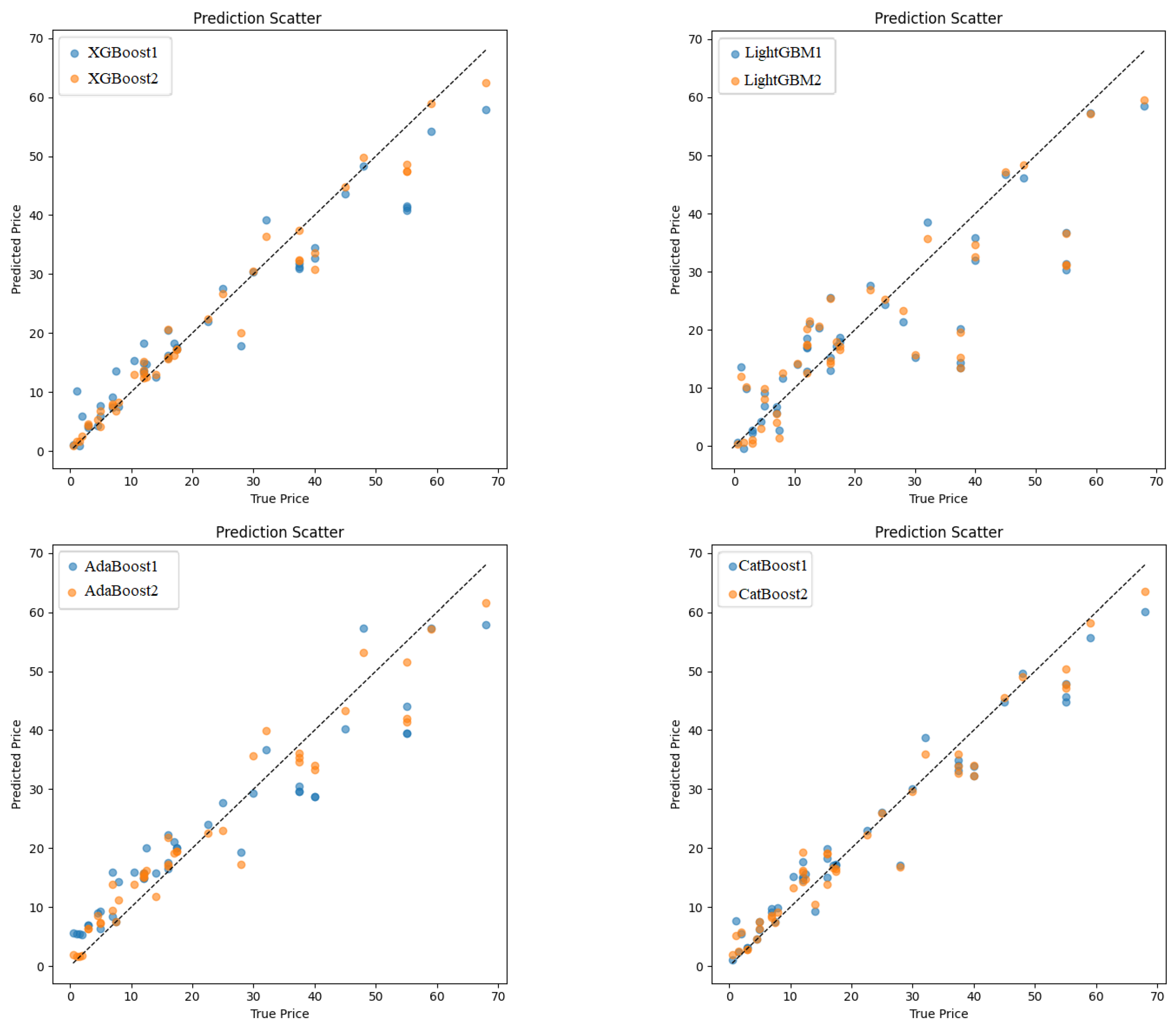
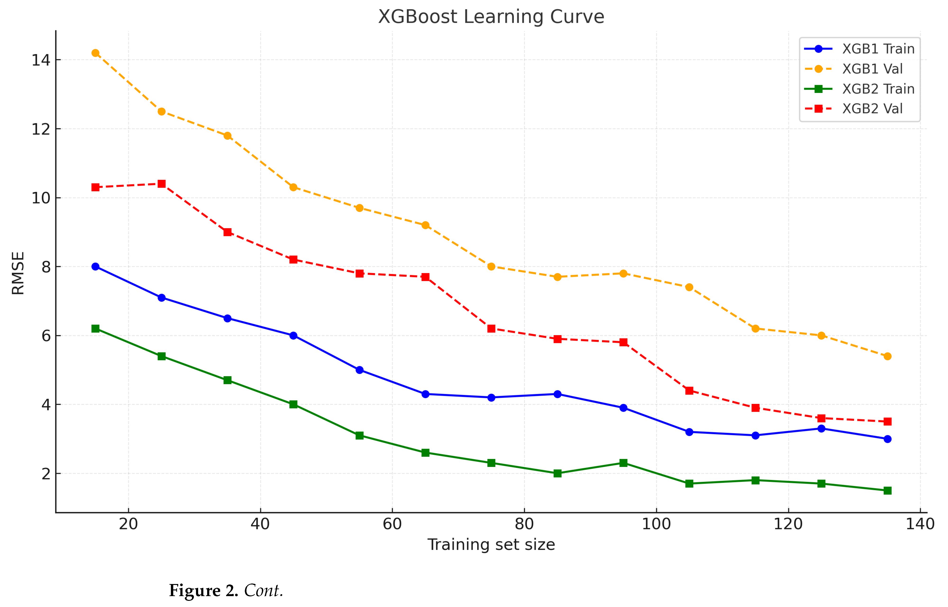
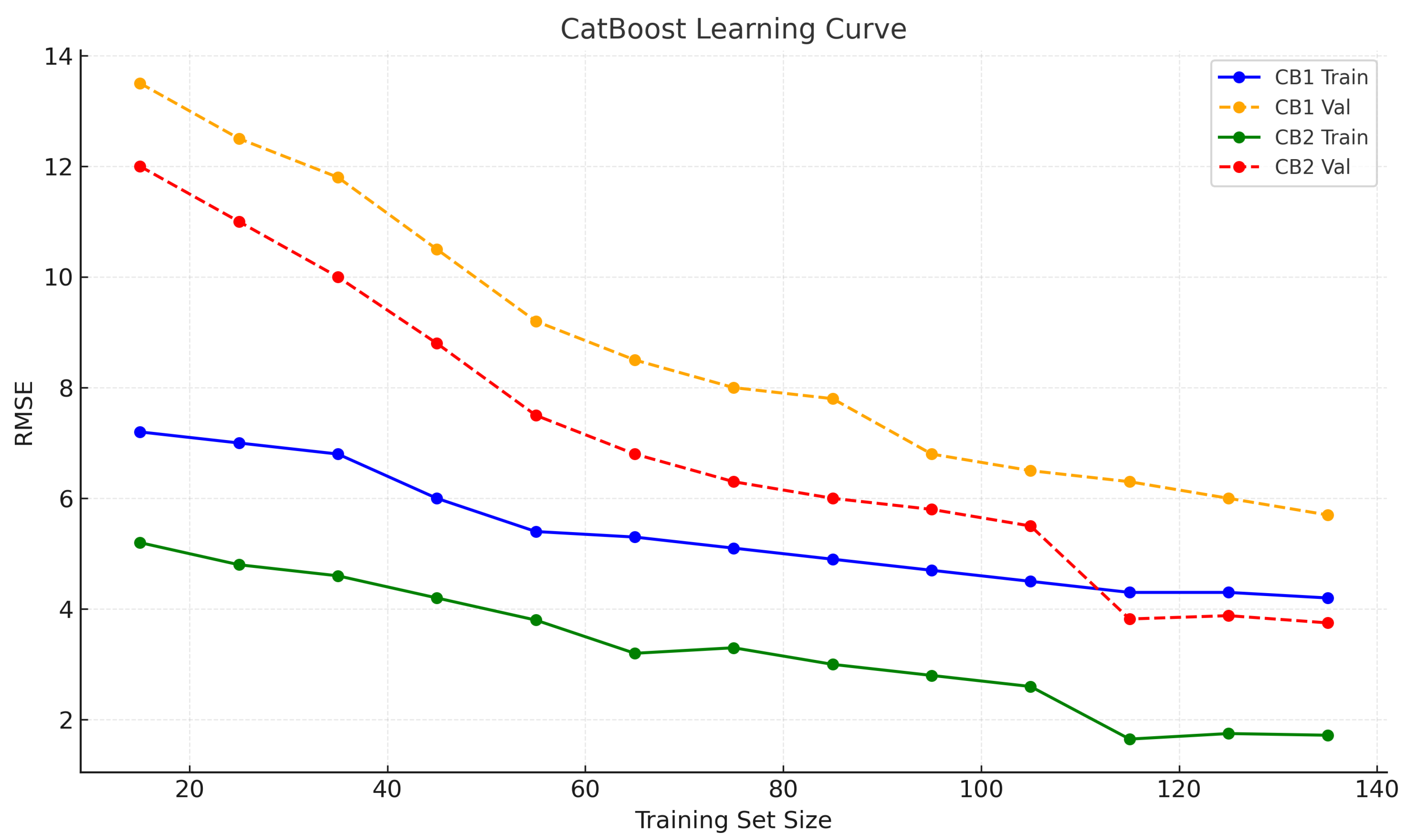
3.1. Optical Imagery Pricing Prediction Results
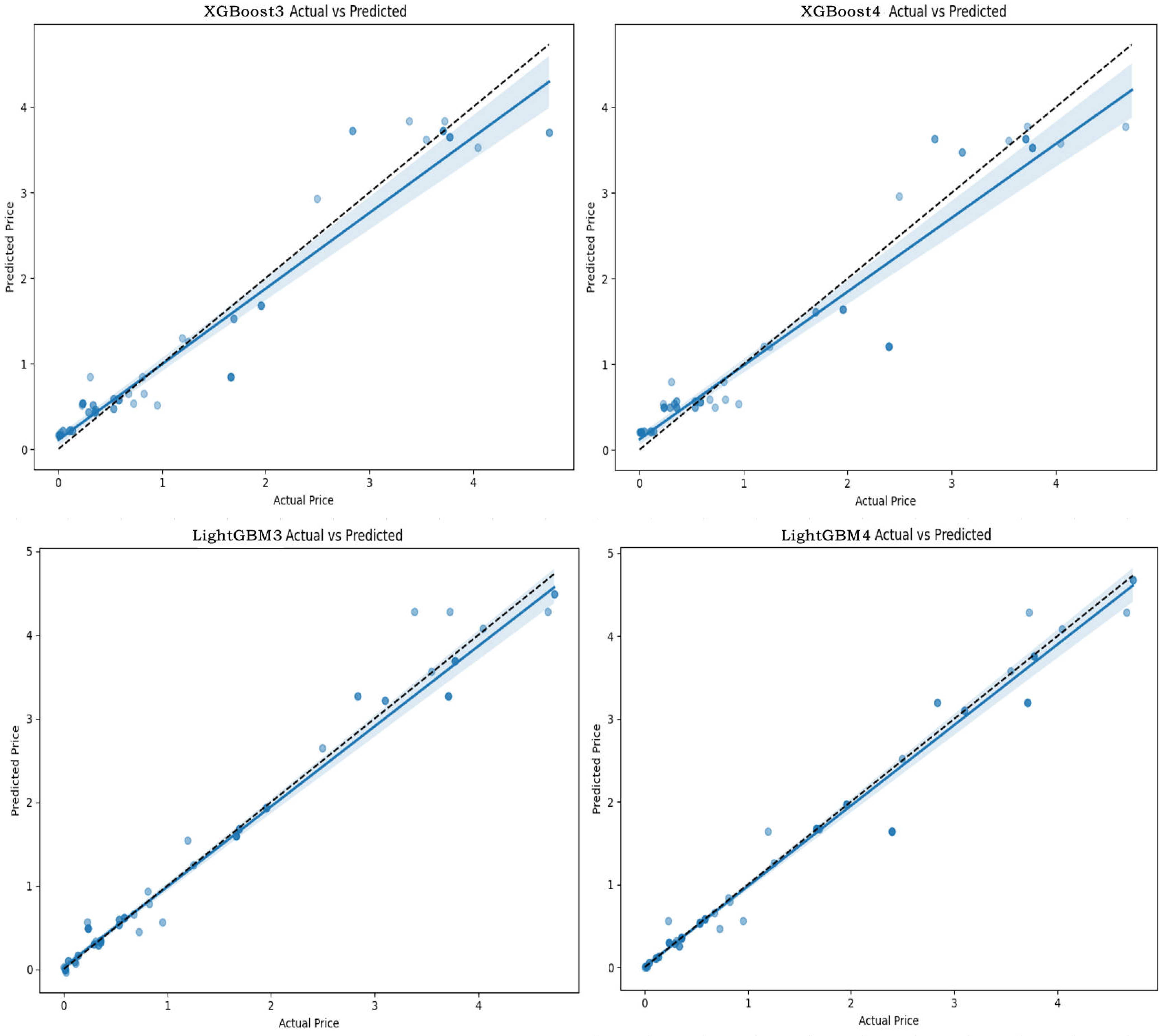
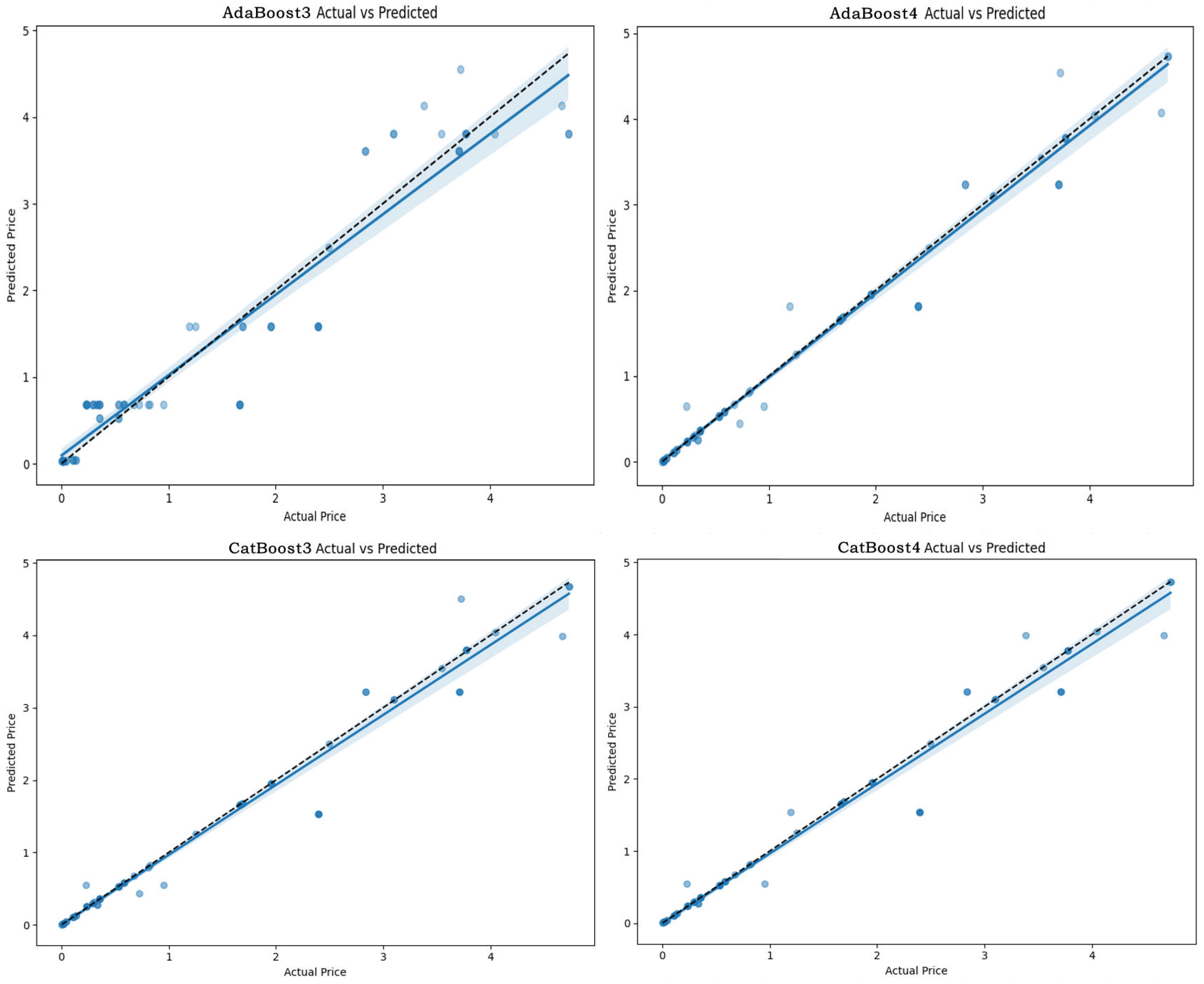
3.1.1. Model Performance Evaluation
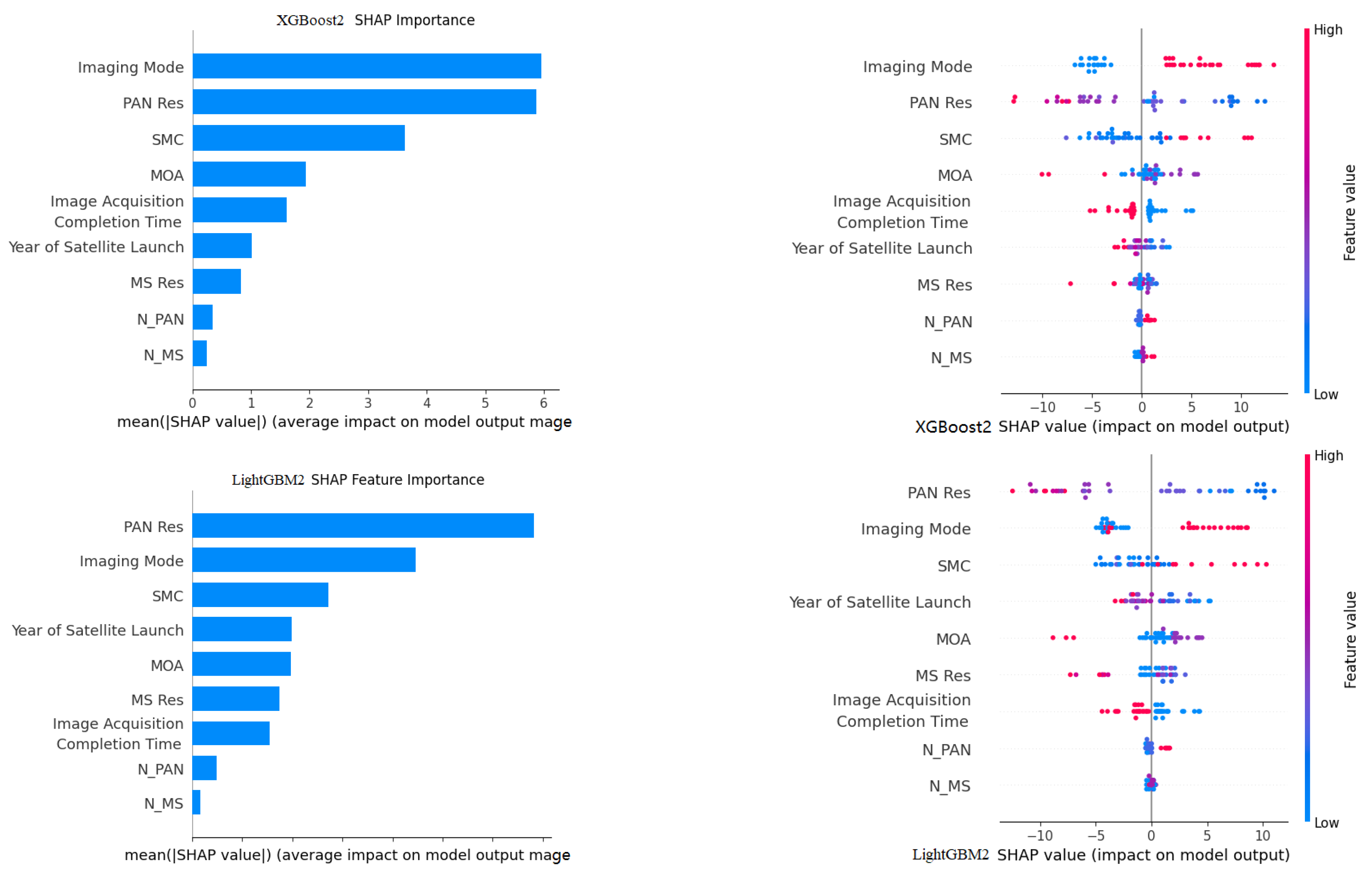
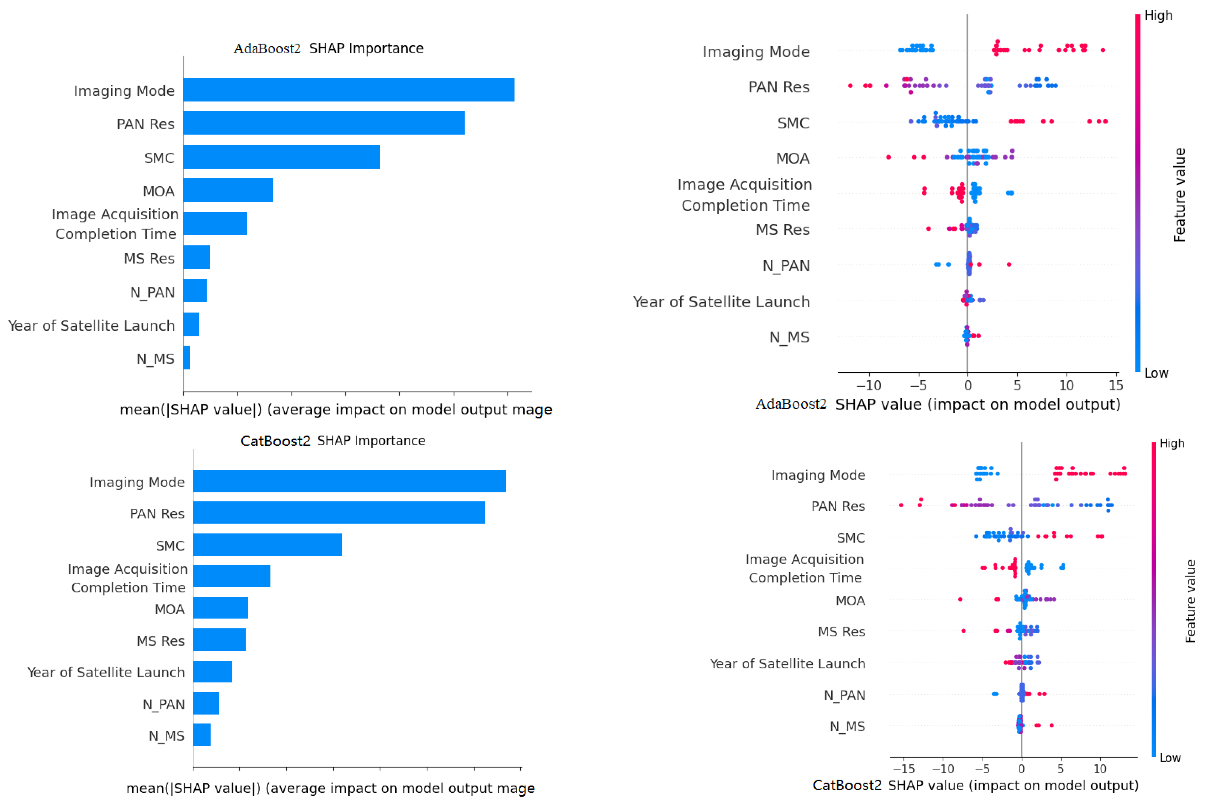
3.1.2. SHAP Feature Importance Analysis
3.2. SAR Imagery Pricing Prediction Results
3.2.1. Model Performance Evaluation
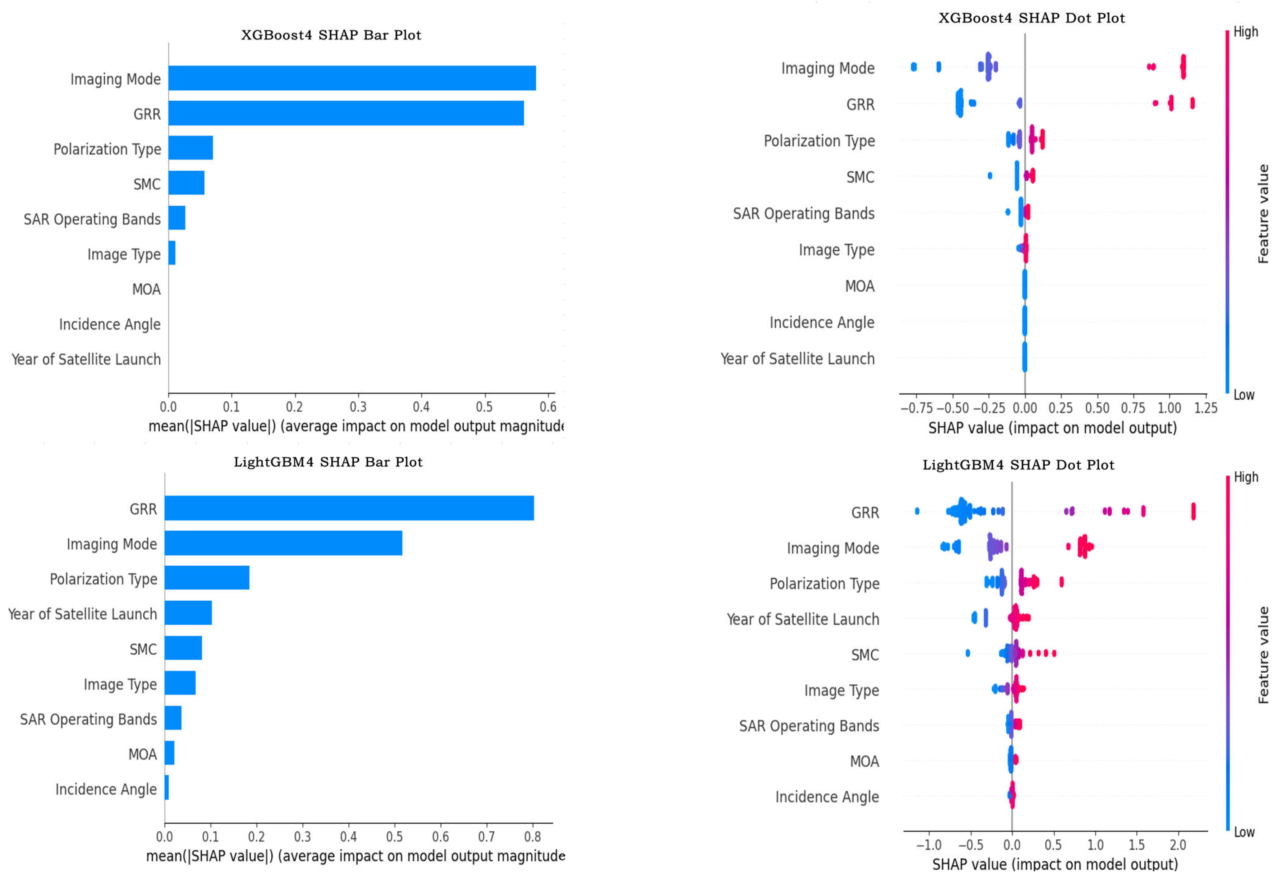
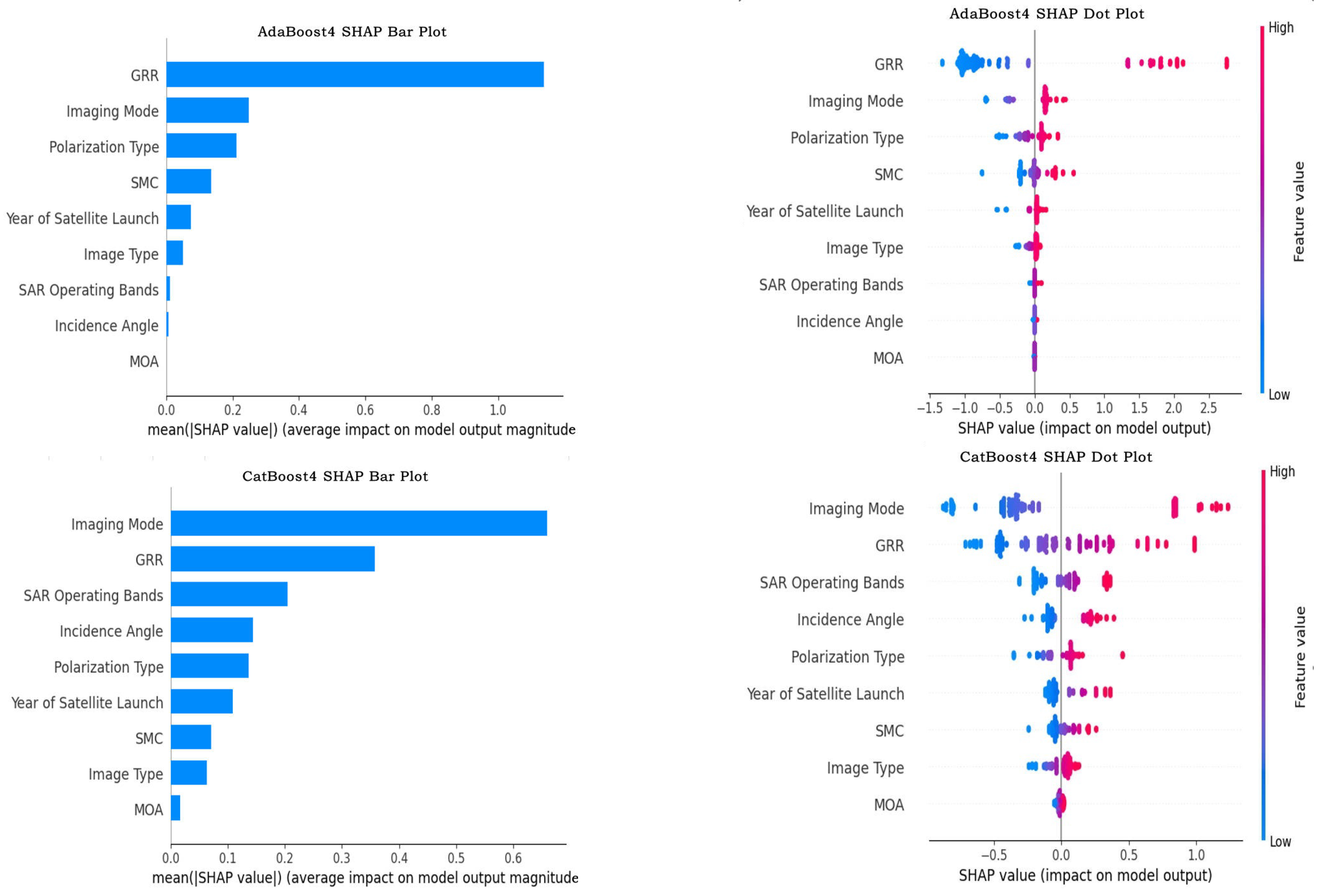
3.2.2. SHAP Feature Importance Analysis
4. Discussion
4.1. Application-Specific Data-Model Alignment
4.1.1. Optical Imagery
4.1.2. SAR Imagery
4.2. Comparison with Traditional Pricing Methods
- Data-Driven Adaptability: Ensemble methods such as XGBoost and CatBoost can ingest dozens of continuous and categorical variables simultaneously, capturing complex, nonlinear interactions—such as the combined effect of sub-meter panchromatic resolution with recent (<90 days) acquisition for urban-infrastructure clients. This yields dynamic price estimates that more accurately reflect supply and demand than fixed rule brackets.
- Hyperparameter Optimization for Robustness:Bayesian optimization systematically tunes regularization strength and tree complexity to minimize overfitting, ensuring strong generalization to unseen data. In contrast, traditional rules lack explicit mechanisms to balance model complexity and bias, often resulting in inconsistent pricing at edge cases.
- Granular Feature-Importance Insights: SHAP analysis quantifies each feature’s marginal economic contribution (e.g., a premium for 30 cm resolution in stereo mode), revealing exactly which attributes drive willingness to pay. Conventional approaches typically treat resolution as a binary “high” vs. “low” toggle and overlook such pricing subtleties.
- Scalability and Real-Time Updating: Once trained, ensemble models can instantly generate quotes for millions of parameter combinations (e.g., any combination of GRR, polarization type, and incidence angle). Manual rule systems cannot adapt without extensive human intervention—a growing limitation in an era of increasingly diverse optical and SAR offerings.
5. Conclusions
Author Contributions
Funding
Data Availability Statement
Acknowledgments
Conflicts of Interest
References
- Herold, M.; Scepan, J.; Clarke, K.C. The Use of Remote Sensing and Landscape Metrics to Describe Structures and Changes in Urban Land Uses. Environ. Plan. A 2002, 34, 1443–1458. [Google Scholar] [CrossRef]
- Choy, S.; Handmer, J.; Whittaker, J.; Shinohara, Y.; Hatori, T.; Kohtake, N. Application of Satellite Navigation System for Emergency Warning and Alerting. Comput. Environ. Urban Syst. 2016, 58, 12–18. [Google Scholar] [CrossRef]
- Kaku, K. Satellite remote sensing for disaster management support: A holistic and staged approach based on case studies in Sentinel Asia. Int. J. Disaster Risk Reduct. 2019, 33, 417–432. [Google Scholar] [CrossRef]
- Rees, G. Physical Principles of Remote Sensing; Cambridge University Press: Cambridge, UK, 2013. [Google Scholar]
- Poursanidis, D.; Chrysoulakis, N. Remote Sensing, natural hazards and the contribution of ESA Sentinels missions. Remote Sens. Appl. Soc. Environ. 2017, 6, 25–38. [Google Scholar] [CrossRef]
- Jordan, H.; Cigna, F.; Bateson, L. Identifying Natural and Anthropogenically-Induced Geohazards from Satellite Ground Motion and Geospatial Data: Stoke-on-Trent, U.K. Int. J. Appl. Earth Obs. Geoinf. 2017, 63, 90–103. [Google Scholar] [CrossRef]
- Shi, S.; Zhong, Y.; Zhao, J.; Lv, P.; Liu, Y.; Zhang, L. Land-use/land-cover change detection based on class-prior object-oriented conditional random field framework for high spatial resolution remote sensing imagery. IEEE Trans. Geosci. Remote Sens. 2020, 60, 1–16. [Google Scholar] [CrossRef]
- Patino, J.E.; Duque, J.C. A Review of Regional Science Applications of Satellite Remote Sensing in Urban Settings. Comput. Environ. Urban Syst. 2013, 37, 1–17. [Google Scholar] [CrossRef]
- Wilhelmi, O.V.; Purvis, K.L.; Harriss, R.C. Designing a Geospatial Information Infrastructure for Mitigation of Heat Wave Hazards in Urban Areas. Nat. Hazards Rev. 2004, 5, 147–158. [Google Scholar] [CrossRef]
- Liu, Y.; Pang, C.; Zhan, Z.; Zhang, X.; Yang, X. Building change detection for remote sensing images using a dual-task constrained deep siamese convolutional network model. IEEE Geosci. Remote Sens. Lett. 2020, 18, 811–815. [Google Scholar] [CrossRef]
- Zhang, B.; Li, Y.; Wang, Z.; Wang, H.; Liu, C.; Ren, J.; Wu, H.; Zhang, L. Progress and Challenges in Intelligent Remote Sensing Satellite Systems. IEEE J. Sel. Top. Appl. Earth Obs. Remote Sens. 2022, 15, 1814–1822. [Google Scholar] [CrossRef]
- Bernknopf, R.; Shapiro, C. Economic Assessment of the Use Value of Geospatial Information. ISPRS Int. J. Geoinf. 2015, 4, 1142–1165. [Google Scholar] [CrossRef]
- Corbane, C.; Politis, P.; Melchiorri, M.; Florczyk, A.J.; Sabo, F.; Freire, S.; Pesaresi, M. Remote Sensing for Mapping Natural Habitats and Their Conservation Status—New Opportunities and Challenges. Int. J. Appl. Earth Obs. Geoinf. 2015, 37, 7–16. [Google Scholar] [CrossRef]
- Schreier, G.; Dech, S. High Resolution Earth Observation Satellites and Services in the Next Decade—A European Perspective. Acta Astronaut. 2005, 57, 520–533. [Google Scholar] [CrossRef]
- Dial, G.; Bowen, H.; Gerlach, F.; Grodecki, J.; Oleszczuk, R. IKONOS Satellite, Imagery, and Products. Remote Sens. Environ. 2003, 88, 23–36. [Google Scholar] [CrossRef]
- Laxminarayan, R.; Macauley, M.K. The Value of Information: Methodological Frontiers and New Applications in Environment and Health; Springer Science & Business Media: New York, NY, USA, 2012. [Google Scholar]
- Venkatachalam, L. The Contingent Valuation Method: A Review. Environ. Impact Assess. Rev. 2004, 24, 89–124. [Google Scholar] [CrossRef]
- Tyrväinen, L.; Väänänen, H. The Economic Value of Urban Forest Amenities: An Application of the Contingent Valuation Method. Landsc. Urban Plan. 1998, 43, 105–118. [Google Scholar] [CrossRef]
- Botelho, A.; Pinto, L.M.C.; Lourenço-Gomes, L.; Valente, M.; Sousa, S. Social Sustainability of Renewable Energy Sources in Electricity Production: An Application of the Contingent Valuation Method. Sustain. Cities Soc. 2016, 26, 429–437. [Google Scholar] [CrossRef]
- Lin, P.-J.; Cangelosi, M.J.; Lee, D.W.; Neumann, P.J. Willingness to Pay for Diagnostic Technologies: A Review of the Contingent Valuation Literature. Value Health 2013, 16, 797–805. [Google Scholar] [CrossRef]
- Loomis, J.; Koontz, S.; Miller, H.; Richardson, L. Valuing Geospatial Information: Using the Contingent Valuation Method to Estimate the Economic Benefits of Landsat Satellite Imagery. Remote Sens. 2015, 81, 647–656. [Google Scholar] [CrossRef]
- Jabbour, C.; Hoayek, A.; Maurel, P.; Rey-Valette, H.; Salles, J.-M. How Much Would You Pay for a Satellite Image? Lessons Learned From French Spatial-Data Infrastructure. IEEE Geosci. Remote Sens. Mag. 2020, 8, 8–22. [Google Scholar] [CrossRef]
- Luo, S.; Pedrycz, W.; Xing, L. Pricing of Satellite Image Data Products: Neutrosophic Fuzzy Pricing Approaches Under Different Game Scenarios. Appl. Soft Comput. 2021, 102, 107106. [Google Scholar] [CrossRef]
- Xu, Y.; Chen, R.; Du, H.; Chen, M.; Fu, C.; Li, Y. Evaluation of Green Space Influence on Housing Prices Using Machine Learning and Urban Visual Intelligence. Cities 2025, 158, 105661. [Google Scholar] [CrossRef]
- Cohen, G.; Aiche, A. Forecasting Gold Price Using Machine Learning Methodologies. Chaos Solitons Fractals 2023, 175, 114079. [Google Scholar] [CrossRef]
- Mouchtaris, D.; Sofianos, E.; Gogas, P.; Papadimitriou, T. Forecasting Natural Gas Spot Prices with Machine Learning. Energies 2021, 14, 5782. [Google Scholar] [CrossRef]
- Harris, M.; Kirby, E.; Agrawal, A.; Pokharel, R.; Puyleart, F.; Zwick, M. Machine Learning Predictions of Electricity Capacity. Energies 2023, 16, 187. [Google Scholar] [CrossRef]
- Nti, I.K.; Adekoya, A.F.; Weyori, B.A. A Comprehensive Evaluation of Ensemble Learning for Stock-Market Prediction. J. Big Data 2020, 7, 20. [Google Scholar] [CrossRef]
- Dichtl, H.; Drobetz, W.; Otto, T. Forecasting Stock Market Crashes via Machine Learning. J. Financ. Stab. 2023, 65, 101099. [Google Scholar] [CrossRef]
- Zhu, R.; Zhong, G.-Y.; Li, J.-C. Forecasting Price in a New Hybrid Neural Network Model with Machine Learning. Expert Syst. Appl. 2024, 249 Pt B, 123697. [Google Scholar] [CrossRef]
- Cao, W.; Liu, Y.; Mei, H.; Shang, H.; Yu, Y. Short-Term District Power Load Self-Prediction Based on Improved XGBoost Model. Eng. Appl. Artif. Intell. 2023, 126 Pt A, 106826. [Google Scholar] [CrossRef]
- Gong, J.; Chu, S.; Mehta, R.K.; Meng, Y.; Zhang, Y. XGBoost Model for Electrocaloric Temperature Change Prediction in Ceramics. Npj Comput. Mater. 2022, 8, 140. [Google Scholar] [CrossRef]
- Chen, T.; Guestrin, C. XGBoost: A Scalable Tree Boosting System. In Proceedings of the 22nd ACM SIGKDD International Conference on Knowledge Discovery and Data Mining, San Francisco, CA, USA, 13–17 August 2016; Volume 22, pp. 785–794. [Google Scholar] [CrossRef]
- Meddage, D.P.P.; Ekanayake, I.U.; Weerasuriya, A.U.; Lewangamage, C.S.; Tse, K.T.; Miyanawala, T.P.; Ramanayaka, C.D.E. Explainable Machine Learning (XML) to Predict External Wind Pressure of a Low-Rise Building in Urban-Like Settings. J. Wind Eng. Ind. Aerodyn. 2022, 226, 105027. [Google Scholar] [CrossRef]
- Meddage, D.P.P.; Mohotti, D.; Wijesooriya, K. Predicting Transient Wind Loads on Tall Buildings in Three-Dimensional Spatial Coordinates Using Machine Learning. J. Build. Eng. 2024, 85, 108725. [Google Scholar] [CrossRef]
- Amjad, M.; Ahmad, I.; Ahmad, M.; Wróblewski, P.; Kamiński, P.; Amjad, U. Prediction of Pile Bearing Capacity Using XGBoost Algorithm: Modeling and Performance Evaluation. Appl. Sci. 2022, 12, 2126. [Google Scholar] [CrossRef]
- Ke, G.; Meng, Q.; Finley, T.; Wang, T.; Chen, W.; Ma, W.; Liu, T.Y. LightGBM: A Highly Efficient Gradient Boosting Decision Tree. Adv. Neural Inf. Process. Syst. 2017, 30, 3146–3154. Available online: https://proceedings.neurips.cc/paper/2017/hash/6449f44a102fde848669bdd9eb6b76fa-Abstract.html (accessed on 4 March 2025).
- Li, L.; Liu, Z.; Shen, J.; Wang, F.; Qi, W.; Jeon, S. A LightGBM-Based Strategy To Predict Tunnel Rockmass Class from TBM Construction Data for Building Control. Adv. Eng. Inf. 2023, 58, 102130. [Google Scholar] [CrossRef]
- Shehadeh, A.; Alshboul, O.; Al Mamlook, R.E.; Hamedat, O. Machine Learning Models for Predicting the Residual Value of Heavy Construction Equipment: An Evaluation of Modified Decision Tree, LightGBM, and XGBoost Regression. Autom. Constr. 2021, 129, 103827. [Google Scholar] [CrossRef]
- Freund, Y.; Schapire, R.E. A Decision-Theoretic Generalization of On-Line Learning and an Application to Boosting. J. Comput. Syst. Sci. 1997, 55, 119–139. [Google Scholar] [CrossRef]
- Busari, G.A.; Lim, D.H. Crude Oil Price Prediction: A Comparison between AdaBoost-LSTM and AdaBoost-GRU for Improving Forecasting Performance. Comput. Chem. Eng. 2021, 155, 107513. [Google Scholar] [CrossRef]
- Prokhorenkova, L.; Gusev, G.; Vorobev, A.; Dorogush, A.V.; Gulin, A. CatBoost: Unbiased Boosting with Categorical Features. Adv. Neural Inf. Process. Syst. 2018, 31, 6638–6648. Available online: https://proceedings.neurips.cc/paper/2018/hash/14491b756b3a51daac41c24863285549-Abstract.html (accessed on 4 March 2025).
- Dong, L.; Zeng, W.; Wu, L.; Lei, G.; Chen, H.; Srivastava, A.K.; Gaiser, T. Estimating the Pan Evaporation in Northwest China by Coupling CatBoost with Bat Algorithm. Water 2021, 13, 256. [Google Scholar] [CrossRef]
- Qian, L.; Chen, Z.; Huang, Y.; Stanford, R.J. Employing Categorical Boosting (CatBoost) and Meta-Heuristic Algorithms for Predicting the Urban Gas Consumption. Urban Clim. 2023, 51, 101647. [Google Scholar] [CrossRef]
- Paulik, C.; Dorigo, W.; Wagner, W.; Kidd, R. Validation of the ASCAT Soil Water Index Using in Situ Data from the International Soil Moisture Network. Int. J. Appl. Earth Obs. Geoinf. 2014, 30, 1–8. [Google Scholar] [CrossRef]
- Morales, P.; Sykes, M.T.; Prentice, I.C.; Smith, P.; Smith, B.; Bugmann, H.; Zierl, B.; Friedlingstein, P.; Viovy, N.; Sabaté, S.; et al. Comparing and Evaluating Process-Based Ecosystem Model Predictions of Carbon and Water Fluxes in Major European Forest Biomes. Glob. Chang. Biol. 2005, 11, 2211–2233. [Google Scholar] [CrossRef] [PubMed]
- Entekhabi, D.; Reichle, R.H.; Koster, R.D.; Crow, W.T. Performance Metrics for Soil Moisture Retrievals and Application Requirements. J. Hydrometeorol. 2010, 11, 832–840. [Google Scholar] [CrossRef]
- Li, L.; Dai, Y.; Shangguan, W.; Wei, Z.; Wei, N.; Li, Q. Causality-Structured Deep Learning for Soil Moisture Predictions. J. Hydrometeorol. 2022, 23, 1315–1331. [Google Scholar] [CrossRef]
- Nash, J.E.; Sutcliffe, J.V. River Flow Forecasting through Conceptual Models Part I—A Discussion of Principles. J. Hydrol. 1970, 10, 282–290. [Google Scholar] [CrossRef]

| No. | Input Variable Name | Variable Type | Encoding Method | Description |
|---|---|---|---|---|
| 1 | Image Acquisition Completion Time | Categorical | One-hot Encoding | Binary classification indicating whether the image acquisition was completed recently (≤90 days) or earlier (>90 days). |
| 2 | Year of Satellite Launch | Continuous | Not encoded | Launch year of the satellite. |
| 3 | Satellite Manufacturing Cost (SMC) | Continuous | Not encoded | Satellite manufacturing cost (billion USD). |
| 4 | Imaging Mode | Categorical | One-hot Encoding | Categorical variable indicating the satellite imaging mode: single-view, stereo-view, or tri-stereo. |
| 5 | Panchromatic Image Resolution (PAN Res) | Continuous | Not encoded | Panchromatic resolution in centimeters (CM). |
| 6 | Number of Panchromatic Bands (N_PAN) | Continuous | Not encoded | Count of panchromatic spectral bands. |
| 7 | Number of Multispectral Bands (N_MS) | Continuous | Not encoded | Count of multispectral spectral bands. |
| 8 | Multispectral Image Resolution (MS Res) | Continuous | Not encoded | Multispectral resolution in centimeters (CM). |
| 9 | Minimum Order Area (MOA) | Continuous | Not encoded | Minimum purchase unit (km2). |
| 10 | Price | Continuous | Not encoded | Satellite imagery price (USD/km2). |
| No. | Input Variable Name | Variable Type | Encoding Method | Description |
|---|---|---|---|---|
| 1 | Year of Satellite Launch | Continuous | Not encoded | Current year minus satellite launch year (years). |
| 2 | Sensor Manufacturing Cost (SMC) | Continuous | Not encoded | Launch year of the satellite (million USD). |
| 3 | Imaging Mode | Categorical | One-hot Encoding | Radar imaging mode: ScanSAR, Spotlight, or Stripmap. |
| 4 | Ground Range Resolution (GRR) | Continuous | Not encoded | Spatial resolution in the range direction (meters). |
| 5 | Polarization Type | Categorical | Multi-Hot Encoding | Polarization type used during acquisition: Single, Dual, or Quad polarization |
| 6 | SAR Operating Bands | Categorical | Multi-Hot Encoding | SAR operating frequency bands, such as L, X, C, P, S, Ku, Ka; multiple bands may be supported simultaneously |
| 7 | Incidence Angle | Continuous | Not encoded | Incidence angle between radar beam and ground (degrees). |
| 8 | Minimum Order Area (MOA) | Continuous | Not encoded | Minimum number of scenes required for order (km2). |
| 9 | Image Type | Categorical | One-hot Encoding | Image type indicating whether the SAR data is from archive or newly tasked acquisition; |
| 10 | Price | Continuous | Not encoded | SAR imagery price (USD/km2). |
| Model | Hyperparameter | Optimal | Default |
|---|---|---|---|
| XGBoost | Learning rate | 0.15 | 0.05 |
| Maximum depth | 5 | 3 | |
| Number of trees | 183 | 200 | |
| Subsample for tree | 0.901 | 0.8 | |
| Depth sample fraction | 0.866 | 0.8 | |
| Regularization (alpha) | 5 | 0 | |
| Regularization (lambda) | 10 | 0 | |
| LightGBM | Number of boosting iterations | 185 | 200 |
| Learning rate | 0.1723 | 0.1 | |
| Number of leaves | 46 | 31 | |
| Maximum depth | 4 | −1 | |
| Min data in leaf | 20 | 20 | |
| Regularization (alpha) | 2.6094 | 2 | |
| Regularization (lambda) | 12.8713 | 5 | |
| AdaBoost | Base Estimator | 5 | 3 |
| Number of Weak Learners | 95 | 50 | |
| Learning Rate | 0.9702 | 1.0 | |
| Loss Function | linear | linear | |
| CatBoost | Number of trees | 1200 | 1000 |
| Learning rate | 0.0949 | 0.03 | |
| Depth of tree | 4 | 4 | |
| Subsample for iteration | 0.8 | 1.0 | |
| Level feature proportion | 0.779 | 1.0 | |
| Regularization | 67.49 | 30 |
| Model | Hyperparameter | Optimal | Default |
|---|---|---|---|
| XGBoost | Learning rate | 0.0981 | 0.05 |
| Maximum depth | 6 | 4 | |
| Number of trees | 185 | 100 | |
| Subsample for tree | 0.8719 | 0.8 | |
| Depth sample fraction | 0.846 | 0.8 | |
| LightGBM | Number of boosting iterations | 100 | 100 |
| Learning rate | 0.270069 | 0.1 | |
| Number of leaves | 54 | 128 | |
| Maximum depth | 8 | 10 | |
| Min data in leaf | 16 | 20 | |
| Regularization (alpha) | 0.9 | 0 | |
| Regularization (lambda) | 0.458 | 0 | |
| AdaBoost | Base Estimator | 5 | 3 |
| Number of Weak Learners | 143 | 50 | |
| Learning Rate | 0.7835 | 1.0 | |
| Loss Function | Linear | linear | |
| CatBoost | Number of trees | 200 | 200 |
| Learning rate | 0.26867 | 0.1 | |
| Depth of tree | 9 | 6 | |
| Subsample for iteration | 0.786 | 1.0 | |
| Level feature proportion | 0.7158 | 1.0 | |
| L2 regularization | 10 | 3 |
| Models | Dataset | R | MBE ($) | RMSE ($) | ubRMSE ($) | NSE | KGE |
|---|---|---|---|---|---|---|---|
| XGBoost1 (Default Parameters) | Training | 0.9820 | 3.1336 | 3.1313 | 0.9613 | 0.9261 | |
| Testing | 0.9697 | 5.5192 | 5.4440 | 0.9101 | 0.7964 | ||
| XGBoost2 (Bayesian Optimized) | Training | 0.9965 | 1.3449 | 1.3449 | 0.9929 | 0.9855 | |
| Testing | 0.9870 | 3.4389 | 3.3420 | 0.9651 | 0.8950 | ||
| LightGBM1 (Default Parameters) | Training | 0.9616 | 0.0017 | 4.4000 | 4.4000 | 0.9238 | 0.9211 |
| Testing | 0.8647 | 9.6777 | 9.3925 | 0.7236 | 0.7170 | ||
| LightGBM2 (Bayesian Optimized) | Training | 0.9640 | 0.0043 | 4.2577 | 4.2577 | 0.9286 | 0.9277 |
| Testing | 0.8669 | 9.5816 | 9.2850 | 0.7290 | 0.7289 | ||
| AdaBoost1 (Default Parameters) | Training | 0.9715 | 1.6241 | 4.5098 | 4.2072 | 0.9199 | 0.8287 |
| Testing | 0.9522 | 0.0513 | 6.5145 | 6.5143 | 0.8747 | 0.7684 | |
| AdaBoost2 (Bayesian Optimized) | Training | 0.9878 | 0.6273 | 2.7615 | 2.6893 | 0.9700 | 0.9146 |
| Testing | 0.9712 | 0.2114 | 4.7942 | 4.7895 | 0.9322 | 0.8634 | |
| CatBoost1 (Default Parameters) | Training | 0.9768 | 3.8078 | 3.8054 | 0.9429 | 0.8689 | |
| Testing | 0.9608 | 6.4326 | 6.3454 | 0.8779 | 0.7483 | ||
| CatBoost2 (Bayesian Optimized) | Training | 0.9951 | 1.6176 | 1.6176 | 0.9897 | 0.9733 | |
| Testing | 0.9826 | 3.8349 | 3.8143 | 0.9566 | 0.8881 |
| Models | Dataset | R | MBE ($) | RMSE ($) | ubRMSE ($) | NSE | KGE |
|---|---|---|---|---|---|---|---|
| XGBoost3 (Default Parameters) | Training | 0.8128 | 14.9660 | 14.6629 | 0.5022 | 0.3124 | |
| Testing | 0.7981 | 19.6583 | 18.6724 | 0.4585 | 0.2801 | ||
| XGBoost4 (Bayesian Optimized) | Training | 0.8154 | 14.0263 | 13.8422 | 0.5628 | 0.4157 | |
| Testing | 0.7984 | 18.5375 | 17.8510 | 0.5185 | 0.3729 | ||
| LightGBM3 (Default Parameters) | Training | 0.9580 | 7.5399 | 7.5105 | 0.8737 | 0.7350 | |
| Testing | 0.8668 | 14.2391 | 14.0447 | 0.7159 | 0.6365 | ||
| LightGBM4 (Bayesian Optimized) | Training | 0.9780 | 5.2519 | 5.2504 | 0.9387 | 0.8427 | |
| Testing | 0.8795 | 13.4476 | 13.2780 | 0.7466 | 0.6770 | ||
| AdaBoost3 (Default Parameters) | Training | 0.8294 | 2.0758 | 10.1853 | 9.9715 | 0.6605 | 0.7446 |
| Testing | 0.8561 | 14.3591 | 14.2416 | 0.7026 | 0.6343 | ||
| AdaBoost4 (Bayesian Optimized) | Training | 0.9153 | 7.1323 | 7.0569 | 0.8335 | 0.8339 | |
| Testing | 0.9258 | 9.9877 | 9.9783 | 0.8561 | 0.8705 | ||
| CatBoost3 (Default Parameters) | Training | 0.9268 | 7.4572 | 7.0259 | 0.8180 | 0.6835 | |
| Testing | 0.9283 | 9.9797 | 9.9348 | 0.8564 | 0.8296 | ||
| CatBoost4 (Bayesian Optimized) | Training | 0.9282 | 7.4694 | 7.0209 | 0.8174 | 0.6764 | |
| Testing | 0.9278 | 9.9384 | 9.9005 | 0.8575 | 0.8443 |
Disclaimer/Publisher’s Note: The statements, opinions and data contained in all publications are solely those of the individual author(s) and contributor(s) and not of MDPI and/or the editor(s). MDPI and/or the editor(s) disclaim responsibility for any injury to people or property resulting from any ideas, methods, instructions or products referred to in the content. |
© 2025 by the authors. Licensee MDPI, Basel, Switzerland. This article is an open access article distributed under the terms and conditions of the Creative Commons Attribution (CC BY) license (https://creativecommons.org/licenses/by/4.0/).
Share and Cite
Yang, L.; Chen, Z.; Li, G. Satellite Image Price Prediction Based on Machine Learning. Remote Sens. 2025, 17, 1960. https://doi.org/10.3390/rs17121960
Yang L, Chen Z, Li G. Satellite Image Price Prediction Based on Machine Learning. Remote Sensing. 2025; 17(12):1960. https://doi.org/10.3390/rs17121960
Chicago/Turabian StyleYang, Linhan, Zugang Chen, and Guoqing Li. 2025. "Satellite Image Price Prediction Based on Machine Learning" Remote Sensing 17, no. 12: 1960. https://doi.org/10.3390/rs17121960
APA StyleYang, L., Chen, Z., & Li, G. (2025). Satellite Image Price Prediction Based on Machine Learning. Remote Sensing, 17(12), 1960. https://doi.org/10.3390/rs17121960