Nonlinear Interactions and Dynamic Analysis of Ecosystem Resilience and Human Activities in China’s Potential Urban Agglomerations

Abstract

Understanding the nonlinear relationship between human activity intensity (HAI) and ecosystem resilience (ER) is crucial for sustainability, yet underdeveloped areas are often overlooked. This study examines the Xuzhou Urban Agglomeration (XZUA) from 2012 to 2022, creating a framework to assess both ER and HAI. Both frameworks utilize multi-source datasets, such as remote sensing, statistical yearbooks, and geospatial data. The ER framework uniquely combines dynamic and static indicators, while the HAI framework differentiates explicit and implicit human activity dimensions. We used spatial analysis, the Optimal Parameter Geodetector (OPGD), and Multi-Scale Geographically Weighted Regression (MGWR) to examine the nonlinear spatiotemporal interaction between HAI and ER. Results show the following: (1) ER exhibited a “shock-recovery” pattern with a net decline of 3.202%, while HAI followed a nonlinear “rise-fall” trend with a net decrease of 0.800%. (2) Spatial mismatches between HAI and ER intensified over time. (3) The negative correlation in high-HAI regions remained stable, whereas neighboring low-HAI areas deteriorated, indicating a spillover effect. (4) OPGD identified the change in HAI (Sen’s slope) as the primary driver of ER change (q = 0.512), with the strongest interaction observed between HAI Sen’s slope and precipitation (q = 0.802). (5) Compared to HAI intensity (mean), its temporal variation had a more spatially stable influence on ER. These findings offer insights for ecological management and sustainable planning in underdeveloped regions, highlighting the need for targeted HAI and ER interventions.

1. Introduction

Rapid urban growth and increased human activities have significantly altered ecosystems in the Anthropocene. One-fifth of marine ecosystems [1] and one-third of protected areas [2] have faced major disturbances, reducing their ability to self-regulate and withstand external shocks [3]. Understanding how human activity intensity (HAI) affects ecosystem resilience (ER) is a core objective of the Sustainable Development Goals (SDGs), particularly under accelerating urbanization and increasing pressures in developing regions [4].

1.1. Conceptual Evolution and Analytical Frameworks of ER

Resilience refers to a system’s capacity to remain stable in the face of disruptions through feedback, adaptive learning, and transformative responses [5]. The concept has evolved through three phases: engineering resilience (returning to pre-disturbance states) [6]; ecological resilience (absorbing shocks and maintaining function) [7,8]; and evolutionary resilience (adapting and innovating across scales) [5,9]. This evolution in resilience thinking has prompted a shift from single-dimensional, static models to complex, dynamic system models.

Resilience assessments have generally followed two trajectories. One emphasizes external system interactions, such as ecological–urban–economic coupling [10,11,12]. The other focuses on internal ecosystem capacities, including absorption, adaptation, and recovery [5,13]. However, inconsistent terminology and assessment methods continue to limit cross-study comparability. Among available models [14,15], the recently proposed Resistance–Adaptability–Recovery (RAR) framework provides a structured, process-oriented perspective to capture long-term resilience dynamics [16]. Drawing conceptually from earlier work on resilience metrics [17], RAR distinguishes three phases: resistance (buffering capacity), adaptability (structural flexibility), and recovery (trajectory toward a stable or improved state). Unlike traditional models such as DPSIR (Drivers, Pressures, States, Impacts, and Responses) [18] or coefficient-based land use weighting [19], RAR explicitly incorporates temporal sequencing and system evolution. Given the cumulative construction pressures in potential urban agglomerations, this framework better captures the long-term ecological consequences of sustained human activity.

1.2. Quantification of HAI and Its Impact on ER

HAI describes the extent to which human actions reshape natural systems. The idea was first introduced by Marsh in Man and Nature [20]. These human activities often manifest as urban sprawl, excessive resource extraction, and emissions of pollutants and waste heat, all of which impose significant pressure on ER [21,22,23]. It is quantified using two main approaches: indirect methods, which rely on proxies like vegetation indices [24] and disturbance indicators [25], and direct methods, which use data such as the Human Footprint Index, nighttime lights, and land use intensity [19,26,27]. The UN New Urban Agenda reports that 54% of the world’s population resided in urban areas in 2014, with an expected increase to 60.4% by 2030 [28]. As a result, HAI has become a key variable in ER-related research [29,30].

Early ER driving studies employed simple correlation and Ordinary Least Squares (OLS) models. More sophisticated approaches have included segmented regressions (e.g., threshold models) and spatial methods such as Geographically Weighted Regression (GWR) [31,32]. More recently, nonlinear models—including Geodetector (GD) and neural networks—have been employed to better capture the complexity and spatial heterogeneity of HAI–ER interactions [16,19,23].

This evolving understanding of HAI reveals a dual role: while often associated with ecological degradation, human activities—if properly managed—may also foster ER and cultural diversity [33]. Such complexity calls for more sophisticated analytical approaches to uncover the nonlinear and spatially heterogeneous dynamics between HAI and ER, especially in the context of rapid urban expansion.

1.3. Potential Urban Agglomeration: XZUA

The 12th Five-Year Plan (2011–2015) first established “ecological security” as a national strategic goal, signaling a shift toward integrated environmental governance [34]. However, despite this strategic goal, China’s urbanization continued unabated. By 2030, the urbanization rate is expected to reach 73%, accompanied by rapid expansion of construction land [35]. This creates a clear tension between ecological protection and urban expansion. Urban agglomerations have since become key units for coordinating spatial planning, infrastructure, and ecological goals [36]. Existing studies mostly focus on large and mature agglomerations, such as the Yangtze River Delta, the Pearl River Delta, and the Chengdu-Chongqing region [13,30,37]. In contrast, smaller or emerging agglomerations—despite their strategic potential—remain underexplored.

The Xuzhou Urban Agglomeration (XZUA) is one of seven nationally designated potential agglomerations. As a representative of small and underdeveloped urban agglomerations, it holds unique value for exploring the dynamics of HAI and ER. The XZUA is characterized by low urban primacy, weak inter-city linkages, and limited functional integration [38]. Unlike developed or rapidly growing regions like the Wuhan Metropolitan Area, the XZUA relies heavily on external economic support and has a highly fluid population [39]. These conditions may heighten the sensitivity of ER to changes in human activity intensity, offering a distinct perspective on urban–ecological interactions.

1.4. Research Gaps, Innovations, and Fundamental Hypotheses

Although increasing efforts have examined the relationship between HAI and ER, several key research gaps persist. First, temporal dynamics are often neglected. Many studies rely on static indicators or single-year observations, failing to capture how long-term changes in HAI shape ER. Even when time-series data are used, interactions are often reduced to pointwise correlations, overlooking cross-temporal feedbacks between systems [5,13,19]. Second, nonlinear responses remain underexplored. Most models assume linearity, limiting the detection of ecological thresholds or tipping points under varying levels of human pressure [16,19,23]. Third, potential urban agglomerations—despite their strategic significance—have rarely been the focus of HAI–ER research.

To address these gaps, this study introduces three methodological innovations: (1) time window-based ER indicators are integrated into the RAR framework, and Sen’s slope is used to construct temporal trends of HAI and ER, replacing static single-year measures; (2) the Optimal Parameter Geodetector (OPGD) model is employed to identify nonlinearities and threshold effects across spatial scales; and (3) a case study of the XZUA offers context-specific insights into HAI–ER dynamics within potential urban agglomerations.

Building on previous evidence of ecological degradation under intensified human pressure [16,19], we assume that HAI generally reduces ER. However, this relationship may exhibit nonlinearity, vary across time, and differ spatially. Accordingly, we propose the following hypotheses: H1: HAI, ER, and their interactions show significant nonlinear and threshold effects over time. H2: The dynamic trend of HAI (measured by Sen’s slope) has a stronger influence on ER than static HAI levels. H3: The spatial relationship between HAI and ER is heterogeneous. Limited synergistic zones may exist beyond spillover effects, and these zones are shaped by local environmental and administrative contexts. To test these hypotheses, this study develops a multi-scale framework that integrates long-term trend analysis and high-temporal-resolution remote sensing. This framework aims to reveal the spatiotemporal coupling and nonlinear mechanisms between HAI and ER, thereby informing ecosystem management in potential urban agglomerations.

2. Materials and Methods

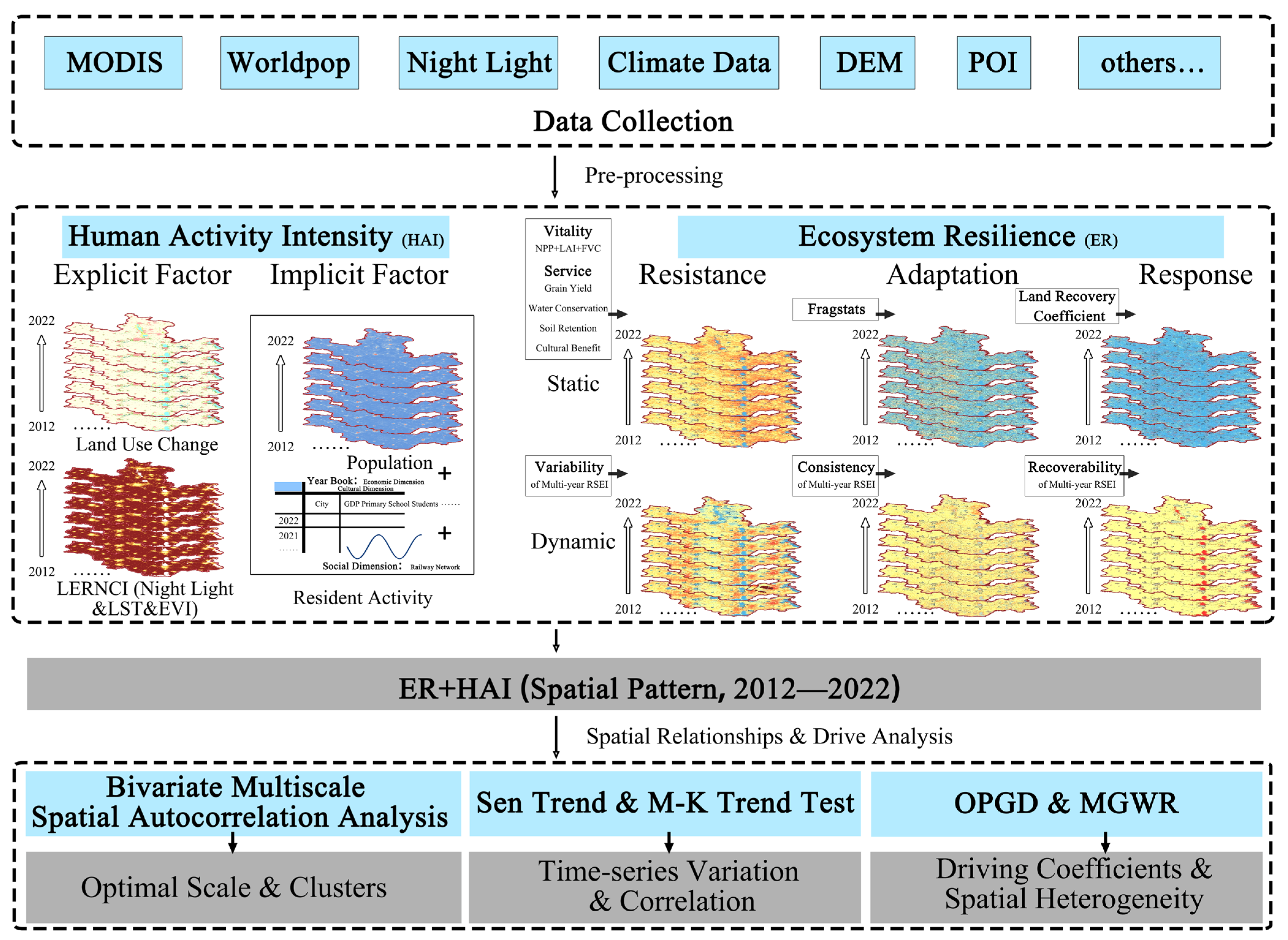
2.1. Flowchart

The research workflow (Figure 1) includes four components: (1) spatial analysis of HAI and ER to reveal distribution and interaction patterns; (2) bivariate multi-scale correlation analysis to examine scale-dependent relationships; (3) trend analysis using Sen’s slope and the Mann–Kendall test on the HAI and ER time series; (4) driving mechanism analysis using OPGD and MGWR. These models assess the effects of both static HAI mean and dynamic HAI trend (Sen’s slope) on ER changes.

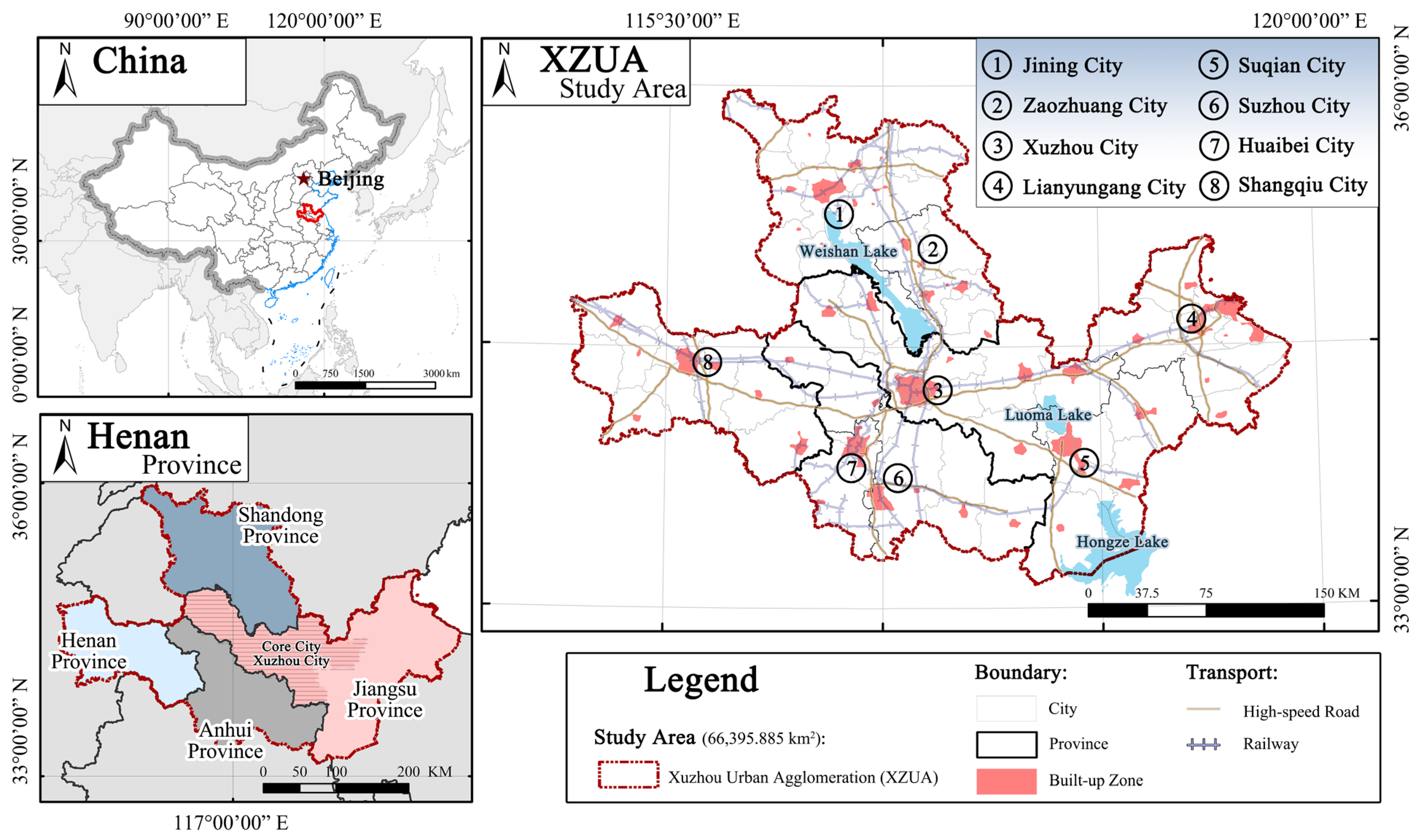
2.2. Study Area

The XZUA covers an area of 66,395.89 km² and spans four provinces—Jiangsu, Shandong, Henan, and Anhui—encompassing eight prefecture-level cities: Xuzhou, Suzhou, Huaibei, Shangqiu, Heze, Jining, Lianyungang, and Zaozhuang (Figure 2) [40]. Geographically, it lies between 117°34′56.78″–121°45′12.45″E and 33°56′12.34″–35°48′22.67″N. The region features diverse terrain types, including coastal and inland zones, plains, and hilly areas. Xuzhou serves as the core city and a major transportation hub in eastern China, supported by an extensive railway and highway network. The ecological environment includes the Huang-Huai-Hai Plain and Weishan Lake Wetland, which support a range of ecosystem services. However, long-term agricultural expansion and urban development have imposed considerable ecological stress on the region. These geographic and ecological conditions provide a valuable context for analyzing human–nature interactions in potential urban agglomerations.

2.3. Data Sources

The data used in this study were derived from a combination of multi-source remote sensing datasets and socio-economic datasets. The primary satellite data included the Terra MODIS Surface Reflectance (SR) dataset, which was used to calculate several remote sensing indices. Although the study period was set to 2012–2022, earlier MODIS data from 2002 onward were also utilized to construct time window-based dynamic indicators. The datasets utilized can be categorized as follows: (1) land use and land cover (LULC): spatial data representing land use patterns and changes; (2) population density (POP): statistical data reflecting population distribution. (3) NOAA VIIRS nighttime light (NTL): data capturing artificial light intensity as a proxy for human activity; (4) land surface temperature (LST): data measuring surface thermal emissions; (5) vegetation indices, including the Normalized Difference Vegetation Index (NDVI), Enhanced Vegetation Index (EVI), leaf area index (LAI), and gross primary productivity (GPP), all derived from MODIS products; (6) meteorological data, including precipitation (Pr), temperature (Tem), surface net solar radiation (SNSR), actual evapotranspiration (AET), and runoff, sourced from meteorological databases; (7) digital elevation model (DEM), obtained from Copernicus DEM datasets; (8) soil erodibility (K Factor), reflecting soil susceptibility to erosion [41]; (9) cultural and tourism resources: point-of-interest (POI) data encompassing Intangible Cultural Heritage (ICH), A-level Scenic Spots (SSs), and Heritage Conservation Units (HCs); (10) socio-economic data, including grain production, tourism revenue, education statistics, and GDP panel data. (11) Unless otherwise specified, all remote sensing data were accessed and processed via the Google Earth Engine platform (GEE, https://code.earthengine.google.com/, accessed on 10 December 2024) (

Table 1. Details about the basic data.

Data	Source	Period	Temporal Resolution	Spatial Resolution
MODIS	GEE, MODIS/061/MOD09A1	2002–2022	8-day	500 m
LULC	GEE, MODIS/061/MCD12Q1 (LC_Type1)	2002–2022	Yearly	500 m
POP	GEE, WorldPop/GP/100m/pop		Yearly	100 m
NTL	GEE, NOAA/VIIRS/001/VNP46A2		Daily	500 m
LST	GEE, MODIS/061/MOD11A2		8-day	1000 m
NDVI	GEE, MODIS/061/MOD13A1		16-day	500 m
EVI
LAI	GEE, MODIS/061/MCD15A3H		4-day	500 m
GPP	GEE, MODIS/061/MOD17A2H		8-day	500 m
Pr	GEE, ECMWF/ERA5_LAND/MONTHLY_BY_HOUR		Monthly	11,132 m
Tem
SNSR
AET	GEE, IDAHO_EPSCOR/TERRACLIMATE		Monthly	4638.3 m
Runoff
DEM	GEE, COPERNICUS/DEM/GLO30	2015	-	30 m
K Factor [42]	(China) National Tibetan Plateau Science Data Center (https://www.tpdc.ac.cn/, accessed on 10 December 2024)	2020	-	25 m
ICH POI	Global Change Research Data Publishing & Repository (https://www.geodoi.ac.cn/, accessed on 2 June 2023)	2011, 2014, 2021	Multi-Year	-
HC POI	National Cultural Heritage Administration Integrated Administrative Platform (http://gl.ncha.gov.cn/, accessed on 2 June 2023)	2019	-	-
SS POI	Provincial Department of Culture and Tourism	2020–2024	Yearly	-
Railway Network	China Basic Geographic Information Database (https://www.webmap.cn/, accessed on 12 December 2024)	2019, 2021	Multi-Year	-
China Urban Statistical Yearbook	(China) National Bureau of Statistics (https://www.stats.gov.cn/, accessed on 12 December 2024)	2013–2023	Yearly	-

).

To ensure spatial and temporal consistency across datasets, we applied a series of preprocessing steps, including cloud removal, annual compositing, spatial resolution standardization (resampled to 500 m), and the imputation of missing values using temporal and spatial neighborhood principles. Population data were corrected using pixel-level regression models and outlier detection via a moving-window IQR test. MODIS land cover data were reclassified into 8 categories to meet analysis needs. Detailed procedures are provided in Appendix A.

2.4. Methods

2.4.1. Multi-Source Data Human Activity Intensity Model

To explore how human activity influences ER, this study constructs a HAI model based on multi-source data. Similar to land use, HAI is divided into two components: explicit intensity, which reflects direct landscape changes, and implicit intensity, which captures latent activity through population and socio-economic factors [43,44]. The final HAI is computed as the mean of the explicit and implicit components:

$$\mathrm{H}\mathrm{A}\mathrm{I}=\mathrm{M}\mathrm{e}\mathrm{a}\mathrm{n}(\mathrm{E}\mathrm{x}\mathrm{p}\mathrm{l}\mathrm{i}\mathrm{c}\mathrm{i}\mathrm{t} \mathrm{H}\mathrm{A}\mathrm{I}+\mathrm{I}\mathrm{m}\mathrm{p}\mathrm{l}\mathrm{i}\mathrm{c}\mathrm{i}\mathrm{t} \mathrm{H}\mathrm{A}\mathrm{I})$$

(1)

(1)

Explicit Indicator

Explicit indicators primarily capture direct changes in the physical environment caused by human activities. These indicators are derived from land use and land cover (LULC) data combined with nighttime light (NTL) imagery. Following previous studies, land use types were converted into construction land equivalents using the Construction Land Equivalent Index (CI) [27]. The CI values were recalibrated to match the land classification system of the XZUA region [19], as shown in

Table A1. Reclassification scheme of MODIS land cover types.

No.	Land Type	Description	CI *	RLC **
1	Forest	Type 1–5, including evergreen needleleaf/broadleaf forests, deciduous needleleaf or broadleaf forests, mixed forests.	0.010	1.000
2	Shrubland	Type 6–7, including closed/open shrublands.	0.133	0.800
3	Grassland	Type 8–10, including woody savannas, savannas, grasslands.	0.067	0.700
4	Wetland	Type 11, including permanent wetlands.	0.067	0.600
5	Farmland	Type 12, 14, including croplands, cropland/natural vegetation mosaics.	0.200	0.500
6	Artificial Surface	Type 13, including urban and built-up lands.	1.000	0.300
7	Barren	Type 16, including barren land.	0.000	0.200
8	Water	Type 15, 17, including permanent snow and ice, water bodies.	0.000	0.800

* CI: Construction Land Equivalent Index; ** RLC: Resilience Land Coefficient. For details on assignment methods, see Section 2.4.1 (1) for CI and Section 2.4.2 (2) for RLC.

.

NTL data are widely recognized as a reliable proxy for human activity intensity. To account for non-light-related activities, we employed the LST and EVI Regulated NTL City Index (LERNCI), which incorporates land surface temperature (LST) and the enhanced vegetation index (EVI) [45]. The formula for explicit HAI is as follows:

$$\mathrm{E}\mathrm{x}\mathrm{p}\mathrm{l}\mathrm{i}\mathrm{c}\mathrm{i}\mathrm{t}\mathrm{H}\mathrm{A}\mathrm{I}=\mathrm{W}1\times \mathrm{C}\mathrm{I}+\mathrm{W}2\times {\mathrm{n}\mathrm{o}\mathrm{r}}^{+}\left(\mathrm{L}\mathrm{E}\mathrm{R}\mathrm{N}\mathrm{C}\mathrm{I}\right),$$

(2)

Here, W represents the weight of the corresponding indicator. Objective weights for each indicator were calculated using the Criteria Importance Through Intercriteria Correlation (CRITIC) method, which jointly considers each indicator’s contrast intensity—measured by its standard deviation—and its level of conflict with other indicators—measured by intercriteria correlation. Indicators with higher variability and lower redundancy (i.e., weaker correlations with others) are assigned higher weights [46] (detailed computation steps are provided in Appendix B.1). Normalization was then performed according to each indicator’s positive or negative contribution to the assessment framework:

$${\mathrm{n}\mathrm{o}\mathrm{r}}^{+}={\displaystyle \frac{\mathrm{X}-{\mathrm{X}}_{\mathrm{m}\mathrm{i}\mathrm{n}}}{{\mathrm{X}}_{\mathrm{m}\mathrm{a}\mathrm{x}}-{\mathrm{X}}_{\mathrm{m}\mathrm{i}\mathrm{n}}}}, {\mathrm{n}\mathrm{o}\mathrm{r}}^{-}={\displaystyle \frac{{\mathrm{X}}_{\mathrm{m}\mathrm{a}\mathrm{x}}-\mathrm{X}}{{\mathrm{X}}_{\mathrm{m}\mathrm{a}\mathrm{x}}-{\mathrm{X}}_{\mathrm{m}\mathrm{i}\mathrm{n}}}}$$

(3)

Here, nor⁺ is used to normalize positive indicators, and nor⁻ is for normalizing negative indicators. X stands for the original data point, while X_min and X_max are the dataset’s minimum and maximum values.

(2)

Implicit Indicator

Implicit indicators, in contrast, are derived from population (POP) data and further capture the Activity Level (AL) of the population, which reflects the degree of engagement in urban life. AL is measured across three dimensions: (1) social—measured by railway network density [47]; (2) economic—represented by two yearbook index-derived indicators (per capita GDP and per capita retail sales) [48,49]; (3) cultural—represented by the proportion of primary school students in the total population and per capita library book collections (Yearbook). The formulas for AL and implicit HAI are as follows:

$$\mathrm{I}\mathrm{m}\mathrm{p}\mathrm{l}\mathrm{i}\mathrm{c}\mathrm{i}\mathrm{t} \mathrm{H}\mathrm{A}\mathrm{I}=\mathrm{P}\mathrm{O}\mathrm{P}\times \mathrm{A}\mathrm{L}=\mathrm{P}\mathrm{O}\mathrm{P}\times {\sum }_{\mathrm{s}=1}^{\mathrm{i}}{\mathrm{W}}_{\mathrm{i}}\times {\mathrm{n}\mathrm{o}\mathrm{r}}^{+}\left(\mathrm{I}\mathrm{n}\mathrm{d}\mathrm{i}\mathrm{c}\mathrm{a}\mathrm{t}\mathrm{o}\mathrm{r}\right)$$

(4)

Here, W_i represents the weight assigned to each indicator, and nor⁺ (Indicator) denotes the normalized value of the corresponding indicator.

2.4.2. Ecosystem Resilience Assessment Framework

This study adopts an “evolutionary resilience” perspective, focusing on an ecosystem’s capacity to buffer risks, adapt to external disturbances, and recover successfully (https://www.resalliance.org/resilience, accessed on 10 February 2025). Accordingly, we utilize the framework of RAR to evaluate ER [16]:

$$\mathrm{E}\mathrm{R}=\sqrt[3]{{\mathrm{n}\mathrm{o}\mathrm{r}}^{+}\left(\mathrm{R}\mathrm{e}\mathrm{s}\mathrm{i}\mathrm{s}\mathrm{t}\mathrm{a}\mathrm{n}\mathrm{c}\mathrm{e}\right)\times {\mathrm{n}\mathrm{o}\mathrm{r}}^{+}\left(\mathrm{A}\mathrm{d}\mathrm{a}\mathrm{p}\mathrm{t}\mathrm{a}\mathrm{t}\mathrm{i}\mathrm{o}\mathrm{n}\right)\times {\mathrm{n}\mathrm{o}\mathrm{r}}^{+}\left(\mathrm{R}\mathrm{e}\mathrm{c}\mathrm{o}\mathrm{v}\mathrm{e}\mathrm{r}\mathrm{y}\right)}$$

(5)

To emphasize the inherent “dynamics” of resilience, this study incorporates historical data within a defined time window as dynamic indicators, complementing traditional static metrics. Therefore, the ER framework consists of two parts, a conventional static assessment framework and a dynamic framework introduced in this research:

$$\mathrm{R}\mathrm{e}\mathrm{s}\mathrm{i}\mathrm{s}\mathrm{t}\mathrm{a}\mathrm{n}\mathrm{c}\mathrm{e}/\mathrm{A}\mathrm{d}\mathrm{a}\mathrm{p}\mathrm{t}\mathrm{a}\mathrm{t}\mathrm{i}\mathrm{o}\mathrm{n}/\mathrm{R}\mathrm{e}\mathrm{c}\mathrm{o}\mathrm{v}\mathrm{e}\mathrm{r}\mathrm{y}=\mathrm{M}\mathrm{e}\mathrm{a}\mathrm{n}(\mathrm{S}\mathrm{t}\mathrm{a}\mathrm{t}\mathrm{i}\mathrm{c} \mathrm{I}\mathrm{n}\mathrm{d}\mathrm{i}\mathrm{c}\mathrm{a}\mathrm{t}\mathrm{o}\mathrm{r}+\mathrm{D}\mathrm{y}\mathrm{n}\mathrm{a}\mathrm{m}\mathrm{i}\mathrm{c} \mathrm{I}\mathrm{n}\mathrm{d}\mathrm{i}\mathrm{c}\mathrm{a}\mathrm{t}\mathrm{o}\mathrm{r})$$

(6)

This integration of dynamic and static indicators allows for a more comprehensive evaluation of ER, capturing both temporal and spatial dimensions of ecosystem responses to disturbances.

(1)

Static Indicator

Resistance: It is closely tied to ecosystem vitality (EV) and ecosystem services (ES), reflecting a system’s self-sustaining and support capacities, respectively [19]. The formula for resistance is

$$\mathrm{S}\mathrm{t}\mathrm{a}\mathrm{t}\mathrm{i}\mathrm{c} \mathrm{R}\mathrm{e}\mathrm{s}\mathrm{i}\mathrm{s}\mathrm{t}\mathrm{a}\mathrm{n}\mathrm{c}\mathrm{e}=\sqrt{{\mathrm{n}\mathrm{o}\mathrm{r}}^{+}\left(\mathrm{E}\mathrm{S}\right)\times {\mathrm{n}\mathrm{o}\mathrm{r}}^{+}\left(\mathrm{E}\mathrm{V}\right)}$$

(7)

EV indicates vegetation growth and productivity, typically measured using NDVI and derived metrics [50], such as annual maximum NDVI values [19]. To address NDVI saturation, additional indicators such as fractional vegetation cover (FVC), leaf area index (LAI), and gross primary productivity (GPP) are included (HJ 1172-2021):

$$\mathrm{E}\mathrm{V}=\mathrm{M}\mathrm{e}\mathrm{a}\mathrm{n} {(\mathrm{n}\mathrm{o}\mathrm{r}}^{+}\left(\mathrm{F}\mathrm{V}\mathrm{C}\right)+{\mathrm{n}\mathrm{o}\mathrm{r}}^{+}\left(\mathrm{L}\mathrm{A}\mathrm{I}\right)+{\mathrm{n}\mathrm{o}\mathrm{r}}^{+}\left(\mathrm{G}\mathrm{P}\mathrm{P}\right))$$

(8)

There are four categories of ES: supporting, regulating, provisioning, and cultural. For the XZUA, key services include grain yield (GY) [51], water conservation (WC) [52], soil retention (SR), and cultural benefits (CB), reflecting the region’s unique geography dominated by plains and hills, as well as its emphasis on water conservation and soil preservation. Methods for quantifying these services are summarized in

Table 2. Methods of ES qualification.

Service Category	Indicator	Methodology
Support	GY	Measurable Proxies, y = ax + b, where x = ${\mathrm{n}\mathrm{o}\mathrm{r}}^{+}\left(\mathrm{N}\mathrm{D}\mathrm{V}\mathrm{I}\right)$, a is calibrated based on regional GY.
Regulation	WC	Water Balance Equation, Q = P – R − AET, Q is water conservation, P is precipitation, R is runoff, and AET is evapotranspiration.
Provision	SR	RUSLE = R × K × L × S × C × P, accounting for rainfall (R), soil erodibility (K), topographic factors (L, S), and vegetation/management factors (C, P).
Culture	CB	Measurable Proxies, y = ax + b, where x = ${\mathrm{n}\mathrm{o}\mathrm{r}}^{+}\mathrm{P}\mathrm{O}\mathrm{I}$ density; a is calibrated based on regional tourism revenue.

:

Adaptation: The spatial pattern of an ecosystem reflects its structural stability, which is positively correlated with its adaptability [53]. Adaptability metrics are typically derived from landscape heterogeneity and connectivity indices [54]. Landscape patterns describe land texture arrangements, where higher heterogeneity indicates interwoven functions, promoting mixed land use and associated benefits.

Heterogeneity is quantified using Shannon’s Diversity Index (SHDI) and the area-weighted mean patch fractal dimension (PFD). Connectivity considers both cross-type connections at the landscape scale and within-type connections at the class scale, measured using contagion indices (CONTs).

Drawing on prior studies [16,19], the weighting scheme for Equation (9) was designed to reflect the ecological importance of spatial structure. The principles are as follows: (1) landscape-scale metrics are prioritized over class-level metrics to capture broader spatial patterns; (2) cross-type connectivity indices, which represent material and energy flows between land types, receive greater weight than within-type indices; and (3) heterogeneity and connectivity metrics are equally weighted within the same spatial level, as they are considered complementary dimensions of ecological adaptability:

$$\begin{gathered} {\mathrm{P}\mathrm{a}\mathrm{t}\mathrm{t}\mathrm{e}\mathrm{r}\mathrm{n}}_{\mathrm{L}\mathrm{a}\mathrm{n}\mathrm{d}\mathrm{s}\mathrm{c}\mathrm{a}\mathrm{p}\mathrm{e}}=0.25\times {\mathrm{n}\mathrm{o}\mathrm{r}}^{+}\left(\mathrm{S}\mathrm{H}\mathrm{D}\mathrm{I}\right)+0.1\times {\mathrm{n}\mathrm{o}\mathrm{r}}^{+}\left(\mathrm{P}\mathrm{F}\mathrm{D}\right)+0.35\times {\mathrm{n}\mathrm{o}\mathrm{r}}^{+}\left(\mathrm{C}\mathrm{O}\mathrm{N}{\mathrm{T}}_1\right) \\ {\mathrm{P}\mathrm{a}\mathrm{t}\mathrm{t}\mathrm{e}\mathrm{r}\mathrm{n}}_{\mathrm{C}\mathrm{l}\mathrm{a}\mathrm{s}\mathrm{s}}=0.1\times {\mathrm{n}\mathrm{o}\mathrm{r}}^{+}\left(\mathrm{C}\mathrm{O}\mathrm{N}{\mathrm{T}}_2\right)+0.1\times {\mathrm{n}\mathrm{o}\mathrm{r}}^{+}\left(\mathrm{C}\mathrm{O}\mathrm{N}{\mathrm{T}}_3\right)+0.1\times {\mathrm{n}\mathrm{o}\mathrm{r}}^{+}\left(\mathrm{C}\mathrm{O}\mathrm{N}{\mathrm{T}}_4\right) \\ \mathrm{S}\mathrm{t}\mathrm{a}\mathrm{t}\mathrm{i}\mathrm{c} \mathrm{A}\mathrm{d}\mathrm{a}\mathrm{p}\mathrm{t}\mathrm{a}\mathrm{t}\mathrm{i}\mathrm{o}\mathrm{n}={\mathrm{P}\mathrm{a}\mathrm{t}\mathrm{t}\mathrm{e}\mathrm{r}\mathrm{n}}_{\mathrm{L}\mathrm{a}\mathrm{n}\mathrm{d}\mathrm{s}\mathrm{c}\mathrm{a}\mathrm{p}\mathrm{e}}+{\mathrm{P}\mathrm{a}\mathrm{t}\mathrm{t}\mathrm{e}\mathrm{r}\mathrm{n}}_{\mathrm{C}\mathrm{l}\mathrm{a}\mathrm{s}\mathrm{s}} \end{gathered}$$

(9)

Here, CONT₁ is contagion at the landscape scale, while CONT₂, CONT₃, and CONT₄ represent class-level connectivity for forests, grasslands, and water.

Recovery: It indicates the system’s capacity to remain stable and bounce back from disruptions. Research indicates that areas near natural ecosystems have a higher likelihood of recovery, whereas human-dominated regions, like built-up areas, may not. Recovery is quantified using resilience coefficients (RLC) assigned to different land use types [19,55]:

$$\mathrm{S}\mathrm{t}\mathrm{a}\mathrm{t}\mathrm{i}\mathrm{c} \mathrm{R}\mathrm{e}\mathrm{c}\mathrm{o}\mathrm{v}\mathrm{e}\mathrm{r}\mathrm{y}={\sum }_{\mathrm{i}=1}^{\mathrm{n}}{\mathrm{R}\mathrm{L}\mathrm{C}}_{\mathrm{i}}\times {\mathrm{A}}_{\mathrm{i}}$$

(10)

Here, ${\mathrm{R}\mathrm{L}\mathrm{C}}_{\mathrm{i}}$ represents the recovery coefficient of the ith LULC, and ${\mathrm{A}}_{\mathrm{i}}$ is the proportional area of that type (Table A1). This traditional approach relies on fixed coefficients derived from expert judgment or empirical estimates, providing a static, land use-based assessment of resilience.

(2)

Dynamic Indicator

Dynamic indicators were constructed using a 10-year time window, with the Remote Sensing Ecological Index (RSEI) as the core metric. This window balances ecological inertia and temporal sensitivity: shorter spans (e.g., 5 years) capture short-term fluctuations but fail to reflect long-term resilience, while longer spans (e.g., 15 years) tend to smooth out early warning signals [56]. Selection details are shown in Section 3.1. To depict the overall ecosystem quality, RSEI merges the NDVI, WET, NDBSI, and LST through principal component analysis [57]. The computational procedure is detailed in Appendix B.2. The dynamic framework consists of the following components [15,58].

Resistance: The resistance indicator reflects not only the intrinsic strength of the ecosystem in resisting external disturbances but also its external performance in response to disturbances over an extended time window. This external performance, termed “Variability,” is a negative indicator used to quantify the ecosystem’s ability to withstand disturbances. Variability is measured using the coefficient of variation (CV):

$$\mathrm{Variability} =\mathrm{C}\mathrm{V}={\mathrm{n}\mathrm{o}\mathrm{r}}^{-}({\displaystyle \frac{\mathrm{S}\mathrm{T}\mathrm{D}}{\mathrm{M}\mathrm{e}\mathrm{a}\mathrm{n}}})$$

(11)

Here, STD and Mean represent the standard deviation and mean of RSEI over the time window, respectively.

Adaptation: Adaptation is assessed by the proportion of high-value years of the RSEI index within the time window, serving as a dynamic suitability indicator for the ecosystem. High-value years are identified using the median absolute deviation (MAD) model. The higher the proportion of high-value periods, the greater the ecosystem’s adaptability:

$$\mathrm{Consistency}={\mathrm{n}\mathrm{o}\mathrm{r}}^{+}({\displaystyle \frac{\mathrm{O}\mathrm{u}\mathrm{t}\mathrm{l}\mathrm{i}\mathrm{e}\mathrm{r} \mathrm{Y}\mathrm{e}\mathrm{a}\mathrm{r}}{\sum \mathrm{T}\mathrm{i}\mathrm{m}\mathrm{e} \mathrm{W}\mathrm{i}\mathrm{n}\mathrm{d}\mathrm{o}\mathrm{w}}})$$

(12)

In this formula, Outlier Year represents the number of years with values significantly exceeding 2.5 times the MAD threshold, and ∑Time Window denotes the total number of years within the time window.

Recovery: Recovery is quantified by analyzing the trend of RSEI values after the lowest point within the time window. A linear fit is applied to RSEI values following the lowest year, and the slope of the fitted line is extracted as the recovery strength indicator:

$${\mathrm{R}\mathrm{S}\mathrm{E}\mathrm{I}}_{\mathrm{t}}=\mathrm{a}\times \mathrm{t}+\mathrm{b},\mathrm{t}>{\mathrm{t}}_{\mathrm{m}\mathrm{i}\mathrm{n}}$$

(13)

where ${\mathrm{R}\mathrm{S}\mathrm{E}\mathrm{I}}_{\mathrm{t}}$ is the RSEI value at year t; a is the slope of the fitted line, representing the rate of post-disturbance recovery; b is the intercept; ${\mathrm{t}}_{\mathrm{m}\mathrm{i}\mathrm{n}}$ is the year when RSEI reaches its minimum value within the analysis window.

2.4.3. Sen’s Slope and Mann–Kendall Test Model

Using multi-year HAI and ER data, Sen’s slope method (Theil–Sen estimator) was applied in ArcGIS Pro 3.0 to calculate trends in HAI and ER. This method calculates the slope between every pair of observations and uses the median slope as the trend estimate [59]. Specifically, for any two points (x_i, y_i) and (x_j, y_j), the slope is computed as follows:

$${\mathrm{S}}_{\mathrm{i}\mathrm{j}}={\displaystyle \frac{{\mathrm{y}}_{\mathrm{j}}-{\mathrm{y}}_{\mathrm{i}}}{{\mathrm{x}}_{\mathrm{j}}-{\mathrm{x}}_{\mathrm{i}}}}$$

(14)

The median of all computed slopes is then taken as the final trend estimate. For monotonic trend detection, the Mann–Kendall (M-K) method was employed. This method assesses the presence and direction of a trend in time series data by calculating the M-K statistic S, which reflects the trend’s strength and direction: S > 0 indicates an upward trend; S < 0 indicates a downward trend; S = 0 indicates no trend. The significance of the trend is determined by calculating the p-value [60]. In this study, a more relaxed significance threshold (p < 0.1) was adopted to support the subsequent driver analysis.

2.4.4. MGWR and OPGD Models

To account for spatial non-stationarity in the relationship between HAI and ER, the Multi-Scale Geographically Weighted Regression (MGWR) model was applied. MGWR extends traditional GWR by assigning each explanatory variable an independently optimized spatial bandwidth, allowing effects to vary across space. Model fitting was conducted using MGWR 2.2, with bandwidths selected via the Golden Section Search algorithm based on AICc minimization [61]. Variables with smaller bandwidths exhibit stronger local variation, while larger bandwidths suggest spatially consistent effects [62]. Control variables (terrain and climate) were included to isolate the net impact of HAI.

To assess nonlinear and interactive effects, we employed the Optimal Parameter Geographical Detector (OPGD), which improves upon the traditional GD method by optimizing the discretization strategy and category number [63]. The OPGD model estimates both the independent explanatory power of each factor (via the q-value) and the interaction effects between factor pairs [64].

Detailed model formulations, parameter settings, and diagnostic metrics are provided in Appendix B.3 (MGWR) and Appendix B.4 (OPGD).

2.4.5. Bivariate Spatial Autocorrelation

Bivariate spatial autocorrelation analysis evaluates the spatial dependency between two variables. In this study, the bivariate Moran’s I coefficient was calculated using the GeoDa and ArcGIS Pro platforms to assess the spatial correlation between ER and HAI. This method identifies how these variables influence each other spatially and reveals the patterns of their interactions [65].

The results are categorized into four types of spatial clustering: HH (high–high) clustering; LL (low–low) clustering; HL (high–low) outliers; LH (low–high) outliers. By distinguishing these spatial patterns, the analysis provides critical insights into the interactions between ER and HAI across different regions, highlighting areas of alignment, divergence, and potential mismatches.

3. Results

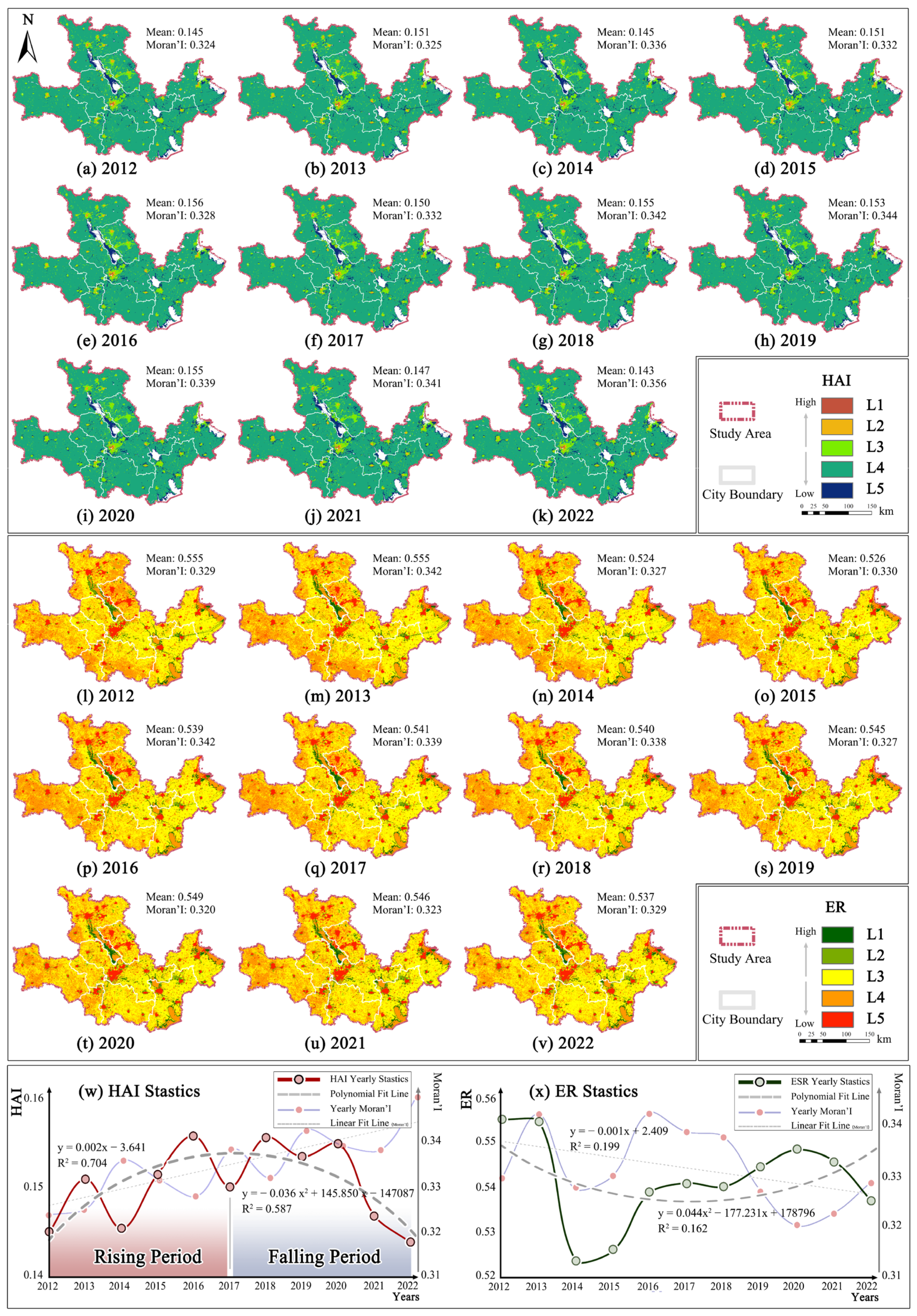
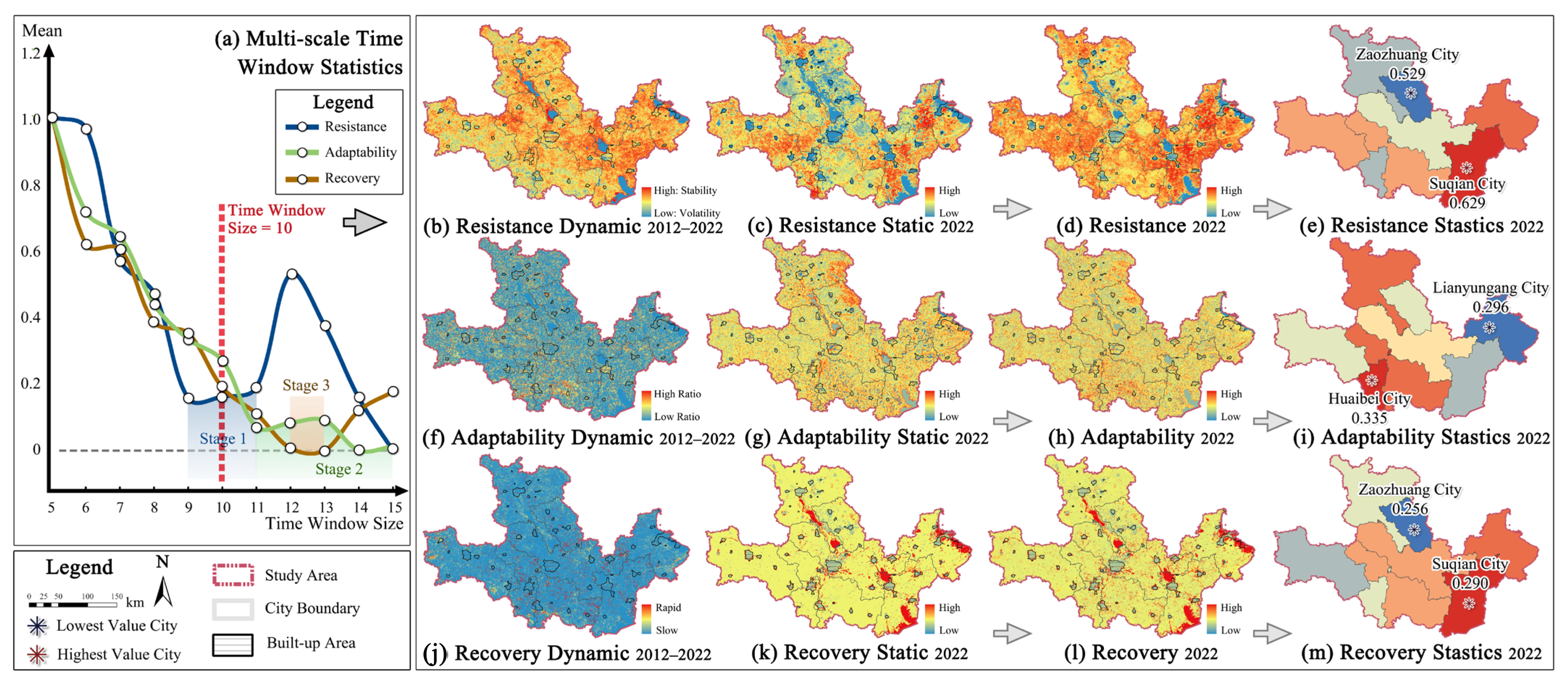
3.1. HAI and ER Assessment Results

Figure 3 presents the integrated evaluation results for both HAI and ER across the study area. For HAI, the Moran’s I index increased from 0.324 to 0.356, indicating an increasingly clustered spatial pattern, with human activities concentrating toward urban areas. Globally, a nonlinear “rise–fall” trend was observed (Figure 3w), with an increase between 2012 and 2017, followed by a gradual decline. The net change in HAI over the study period was –0.800%.

In parallel, the temporal analysis of ER showed a generally stable spatial aggregation pattern, as indicated by its Moran’s I. High-ER regions were primarily located around the Weishan Lake wetlands. In contrast, low-ER zones were mostly confined to built-up areas, especially within Xuzhou’s core, where the most distinct low-value patches were observed. Temporally, ER demonstrated a distinct “shock-recovery” dynamic (Figure 3x). After a sharp decline in 2013, ER gradually recovered to peak in 2020, then declined again, resulting in a net decrease of 3.202% over the entire period.

Using 2022 as the reference year, a 5–15-year moving window analysis was performed, revealing a general decline in all three dynamic ER indicators. Resistance decreased most rapidly and stabilized at its lowest level—indicating maximum ER variability—between the 9- and 11-year windows (Figure 4a, Stage 1). Adaptability remained low and stable from years 11 to 15 (Figure 4a, Stage 2), although resistance fluctuated significantly during this period. Recovery maintained a consistently low value between years 12 and 13 (Figure 4a, Stage 3). Considering both indicator behavior and consistency with the static assessment period, a 10-year window was selected for ER dynamics in this study.

The spatial distribution and descriptive statistics of the three sub-indices of ER—resistance, adaptation, and recovery—are shown in Figure 4. Due to the predominantly flat terrain, none of the sub-indices exhibited pronounced hot or cold spots. No clear clustering cores were observed at the regional scale. Both resistance and recovery showed similar spatial trends, with Zaozhuang recording the lowest values (0.529 and 0.256, respectively) and Suqian achieving the highest (0.629 and 0.290, respectively). For the adaptation index, Huaibei demonstrated the highest value (0.335), while Lianyungang registered the lowest (0.296).

3.2. Spatial Pattern and Correlation Analysis

3.2.1. Shift in Center of Gravity Analysis

Figure 5 shows the spatial shifts of the centers of gravity for HAI and ER. The center for HAI remained near Xuzhou’s urban core, shifting slightly eastward, with a maximum displacement of less than 500 m (Figure 5(a1)). Similarly, the center for ER was located near Xuzhou’s urban core and shifted southward, with a maximum movement of under 700 m (Figure 5(a2)). From 2012 to 2022, Zaozhuang exhibited the highest HAI and lowest ER. In contrast, Suzhou recorded the lowest HAI, while Suqian had the highest ER (Figure 5b–g). Additionally, the centers of gravity for HAI and ER were approximately 6000 m apart. The major axes of the standard deviation ellipses for both indicators were aligned in the northwest–southeast direction.

3.2.2. Multi-Scale Correlation Analysis

In further spatial correlation analysis, the multi-year mean Spearman correlation between HAI and ER reached a stable threshold at the 2000 m scale (∣r∣ = 0.474). Bivariate Moran’s I values for 2012, 2017, and 2022 were –0.296, –0.325, and –0.380, respectively (|z| > 2.58). These results indicate a progressively strengthening spatial negative correlation between HAI and ER. LH (low HAI–high ER) outlier data points constituted the majority, remaining consistently around 1000 points. HL outliers followed, with counts increasing annually from 609 to 737. In contrast, the ideal HH scenario consistently included only about 50 points, while LL cases were more prevalent, reaching approximately 600.

In the multi-scale analysis, the correlation between HAI and ER was strongest at the district-level administrative scale (∣r∣ = 0.526), surpassing correlations at all grid-based scales. At this scale, spatial relationships between HAI and ER were classified into nine scenarios based on intensity levels. Between 2012 and 2022, the number of high-HAI areas (HL/HM) remained stable, while low-HAI areas (LH/LM) experienced a shift in ER from high to moderate levels. As shown in Figure 6e–g, many districts surrounding Xuzhou transitioned from deep blue LH zones to light blue LM zones. This suggests that even in low-HAI areas, ER continued to decline, underscoring the expanding spillover effects of human activity on ER.

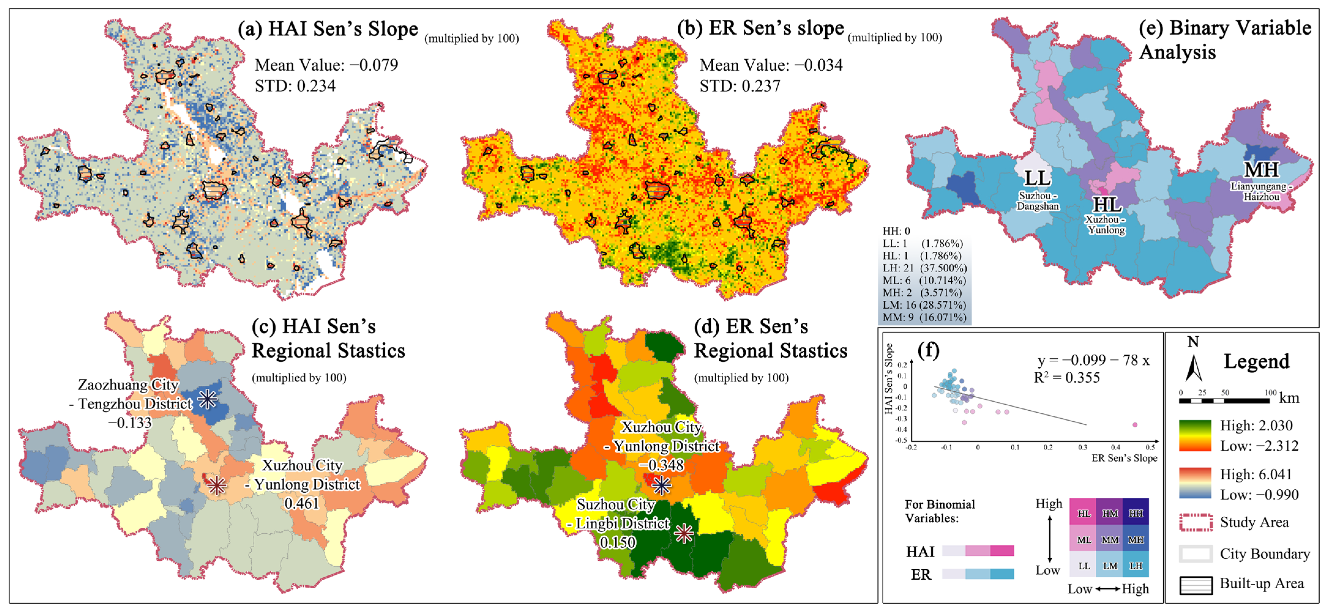
3.3. Trend Analysis

3.3.1. Temporal Dynamics

Based on Sen’s slope analysis (p > 0.1), both HAI and ER exhibited negative global mean trends, indicating overall declines from 2012 to 2022. HAI increases were mainly observed along urban peripheries and major highways—typically in emerging development zones—with a maximum trend of 6.041 × 10⁻² (presented as 6.041 after multiplying by 100 for clarity; Figure 7). In contrast, traditional urban cores and many township areas remained stable or declined slightly. Rural areas—particularly those within Tengzhou District (Zaozhuang) and surrounding counties—showed marked decreases. This spatial pattern aligns with earlier evidence indicating an increasing concentration of human activity in urban centers.

ER declined most severely in high-HAI regions—particularly urban cores and areas with dense road networks. A fitted trend line (y = −78x − 0.099) confirms this pattern. Additional clusters of ER decline were also observed in the northwest farmland regions. In regional correlation analysis, Yunlong District (Xuzhou) showed the most rapid HAI growth and the sharpest ER decline, fitting the HL scenario. Conversely, in low-HAI regions such as Dangshan District (Suzhou, LL scenario), ER continued to decline, highlighting the pervasiveness of ecosystem degradation even under reduced human pressure.

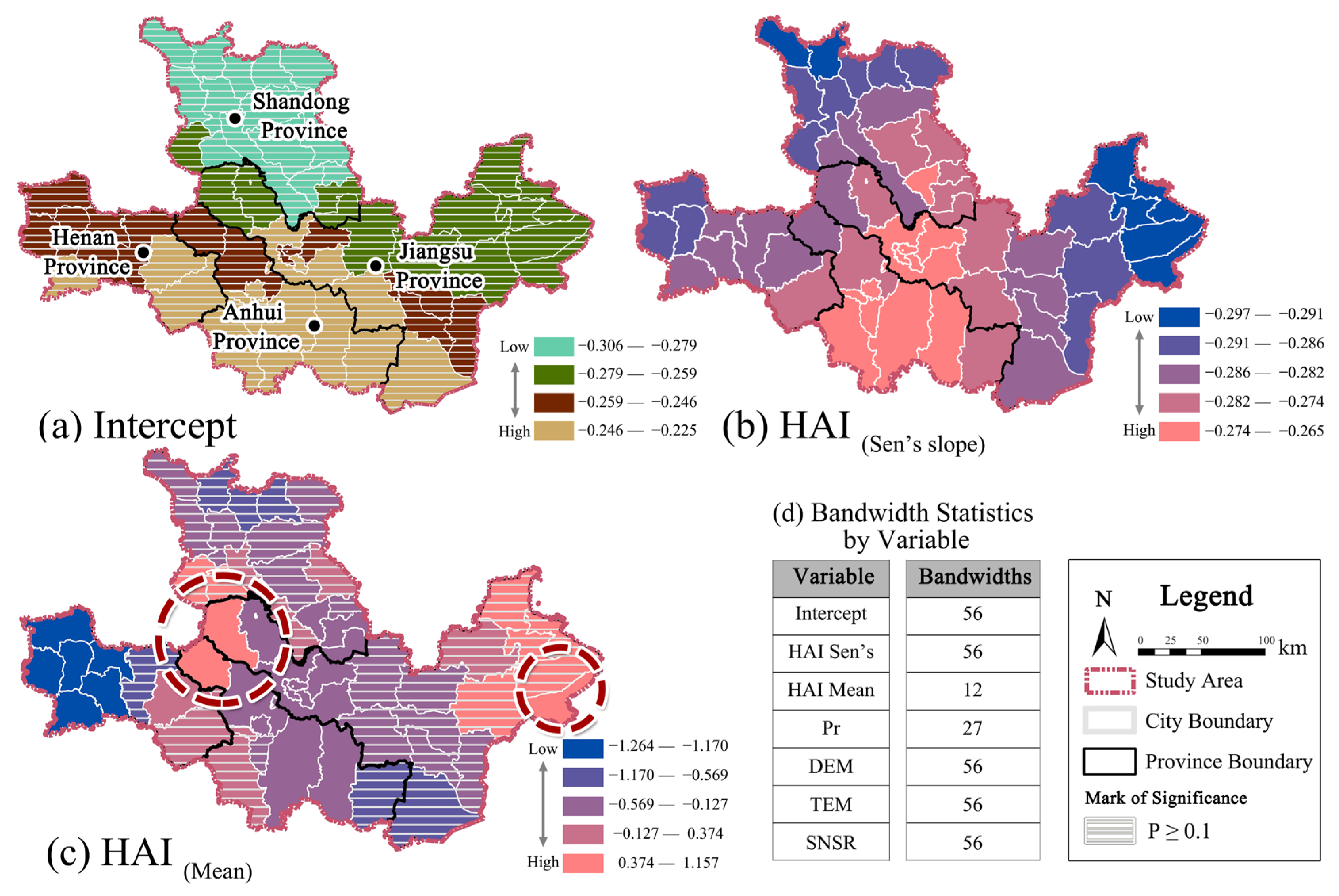
3.3.2. Linear and Non-Linear Driving Analysis

To analyze the drivers of ER Sen’s slope, we included both core explanatory variables—HAI mean and HAI Sen’s slope—and additional controls, including digital elevation model (DEM), precipitation (Pr), temperature (Tem), and surface net solar radiation (SNSR). All variables passed significance tests using Spearman correlation and variance inflation factor (VIF) checks, thereby ruling out multicollinearity (

Table 3. Spearman correlation and VIF results for HAI and control variables.

Variable	HAI Sen’s	HAI Mean	DEM	Rain	Tem	PAR
Spearman Correlation	−0.645 ***	−0.267 **	0.247 *	0.299 **	0.272 **	−0.396 ***
VIF	1.069	1.328	1.617	1.201	1.499	1.077

Note: */**/*** indicate statistical significance at the 10%, 5%, and 1% levels.

).

According to OPGD results, HAI Sen’s slop had the highest q-value (0.512), indicating it was the most significant single-factor driver of ER, surpassing HAI mean, as well as climatic and topographic factors (Figure 8a). The magnitude of change better explains the spatial heterogeneity of ER Sen’s slope than does the absolute strength of HAI. Temperature (q = 0.478) also had a significant effect on ER distribution. While individual natural factors exhibited limited explanatory power, their interactions with anthropogenic variables were substantial, suggesting synergistic effects in shaping ER patterns.

The risk detection analysis (Figure 8b) revealed that within the low-value range of HAI Sen’s slope (0.08–0.09), the mean value of ER Sen’s slope was highest, whereas in the high-value range (0.19–1.00), the mean value of ER Sen’s slope was lowest. The HAI mean indicator exhibited a similar trend in its influence.

In regions with low HAI levels, even minor increases can greatly impact ER, whereas improvements in ER are more probable in areas with moderate HAI/HAI Sen’s levels. As shown in Figure 8c, the interaction between HAI and Pr exhibits a nonlinear enhancement effect, yielding the strongest explanatory combination (q = 0.802) and underscoring drought as a critical factor in the trade-off between human activity and ER.

Introducing MGWR revealed spatial heterogeneity in driver effects (R² = 0.786, AICc = 132.898). The results confirmed that most spatial variations were statistically robust (Figure 9d). HAI Sen’s slope and the intercept were identified as global drivers (bandwidth = 56, 100%, Figure 9a,b), exhibiting consistent effects across the region. In contrast, the HAI mean indicator exhibited strong heterogeneity (bandwidth = 12, 21.429%, Figure 9c), with its influence shifting from negative in western areas to positive in the east. Notably, in several northwestern and eastern regions, high HAI spurred ER growth—deviating from the global trend—while in several western Henan districts, high HAI strongly inhibited ER recovery. The intercept term, representing uncontrolled variables, displayed a north–south gradient influenced by latitude and provincial boundaries, further underscoring the impact of regional policies and geographic context on ER dynamics.

4. Discussion

4.1. Nonlinear Dynamics and Spatiotemporal Mismatch in HAI–ER

This study confirms that the relationship between HAI and ER is fundamentally nonlinear and temporally unstable. By integrating explicit and implicit HAI dimensions with both dynamic and static ER indicators, we reveal human–ecological interactions that deviate from gradual or proportional patterns. The observed inverse correlation between HAI and ER intensifies over time, suggesting that development pressure increasingly exceeds ecological capacity [66,67]. This imbalance may push urban agglomerations toward an environmental Malthusian scenario, where surpassing ecological thresholds renders recovery extremely difficult [68]. In such contexts, urbanization exacerbates ecological stress while limited resilience capacity constrains system adaptation [47].

Temporal patterns reflect distinct nonlinear dynamics. HAI follows an inverted U-shaped trajectory with a net change of –0.800%, whereas ER exhibits a “shock–recovery” trend with a net loss of –3.202%. Although ER partially recovers, it remains below the 2013 baseline. The sudden drop in ER between 2013 and 2014, despite minor HAI fluctuations, points to the existence of ecological thresholds [69]. Such abrupt responses support the notion of switching effects and ecosystem hysteresis, where degradation may escalate nonlinearly under sustained stress [6,70].

Spatially, high-HAI regions—especially around Xuzhou’s urban core and major transport corridors—show consistent ER losses. Urban centers experience severe resilience decline due to land development, infrastructure expansion, and resource overuse [19,66]. In contrast, nonurban areas generally maintain higher ER levels [71]. However, even low-HAI rural zones, particularly in Tengzhou and surrounding townships, exhibit degradation, reflecting indirect pressures and ecological spillovers [72]. These impacts are often driven by upstream land conversion, hydrological disruption, and economic linkages [73,74,75]. This supports earlier findings that ecological risks are interconnected and transmitted across urban areas [76]. Given the cross-regional diffusion of ecological risks, it is insufficient to analyze ecosystem changes based on isolated factors. Instead, integrated and multi-scalar governance strategies are essential to strengthen the stability and adaptive capacity of urban ecological systems [77,78].

4.2. Threshold Effects and Interactive Drivers of HAI Impact

According to the China Population Census Yearbook (2020), regions encompassing the XZUA—such as Henan, Anhui, southern Shandong, and northern Jiangsu—have experienced a net population outflow of approximately 36.22 million. While this demographic decline aligns with a reduction in HAI, ER has not improved accordingly. This disconnect indicates that shrinking cities may still exert ecological pressure due to inefficient infrastructure, outdated industrial systems, and underutilized land [47,72].

To better understand this mismatch, spatial analysis confirms predominantly negative HAI–ER correlations (i.e., HL and LH patterns), consistent with prior findings [29,67] and as shown in Figure 6b–d. OPGD results further indicate that the rate of HAI change (Sen’s slope) is a stronger predictor of ER variation than static levels, with the highest explanatory power among all factors (q = 0.512), surpassing topographic and climatic variables. This highlights the ecological impact of activity dynamics—especially in transitional or peri-urban zones—over absolute intensity alone.

Threshold detection reveals that ER declines sharply when both HAI mean and Sen’s slope exceed 0.59 and 0.19, respectively [31]. In contrast, moderate HAI levels correspond to peak ER, suggesting an optimal activity range within which ecosystems maintain or enhance resilience. These findings counter a strictly antagonistic view of the HAI–ER relationship. Notably, some high-HAI areas, such as parts of the Yangtze River Delta, have shown ER improvement—likely due to sustainability policies, technological upgrades, and ecological restoration [47,50].

These nonlinear effects are not uniformly negative. Between 2012 and 2017, certain areas with rising HAI also exhibited partial ER recovery [19]. This implies that moderate or stable HAI, when managed properly, may even support ecological improvement through urban green infrastructure, land use optimization, and ecological compensation [79,80,81]. Over 90% of China’s protected areas have shown long-term improvement in ES [82]. This highlights the potential of targeted strategies such as vegetation restoration, zoning management, and government regulation to curb anthropogenic disturbances and restore fragile ecosystems.

Finally, natural factors significantly interact with HAI [83]. Precipitation combined with HAI Sen’s had the strongest joint effect on ER (q = 0.802), while temperature was the second most influential single factor (q = 0.478). Similar patterns in the Yellow River Basin show that favorable climatic conditions can buffer anthropogenic stress [84]. Given that the XZUA is located at the junction of Anhui, Jiangsu, Henan, and Shandong provinces—and a drought-prone agricultural zone [85,86]—these climatic interactions are critical for understanding regional ER dynamics.

4.3. Spatial Drivers and Heterogeneity in HAI–ER Relationships

The MGWR results reveal pronounced spatial heterogeneity in the HAI–ER relationship. The static indicator, HAI mean, exhibits a localized effect with a small bandwidth (12), indicating high spatial variation. In the XZUA, HAI mean is negatively correlated with ER Sen’s slope (r = –0.267) [19,87], but this effect varies across regions. In the west, high HAI levels correspond with ecological degradation, while in eastern coastal zones, moderate HAI increases appear to support resilience. These results indicate that high HAI does not uniformly suppress ER. Instead, the HAI–ER relationship varies in direction and intensity across regions [62,88]. This suggests that the influence is not centered on Xuzhou City, highlighting the core city’s lack of dominance in the XZUA. The inland–coastal economic/geographic division appears more distinct than the city cluster structure.

Such lateral variation—from inland to coastal areas—has also been observed in other urban clusters [5], often linked to differences in urbanization stages and planning maturity [35]. Developed regions benefit from strategic spatial planning and ER investments that buffer environmental pressures. In contrast, underdeveloped zones often suffer from inefficient land use, limited green infrastructure, and weaker institutional capacity, intensifying ecological risks [47]. Alternatively, this divergence may stem from disparities in ES supply—regions unable to meet concentrated human demands are more prone to degradation [89].

HAI Sen’s slope, reflecting temporal fluctuations in human activity, acts as a global explanatory factor (Bandwidth = 56) and shows a much stronger negative correlation with ER Sen’s slope (r = –0.645). This implies that rapid or unstable growth in human activity poses greater ecological stress than sustained high levels. Population mobility, a hallmark of urbanization, plays a key role in this dynamic by intensifying human–environment interactions [90]. According to the Environmental Kuznets Curve (EKC) and typical urban trajectories, cities in rapid-growth stages (30–70% urbanization) often undergo resource depletion and ecological decline before achieving sustainability [88,91]. However, for potential urban agglomerations like the XZUA, such a shift is not automatic. Without proactive governance, long-term ecological investment, and effective land use coordination, cumulative pressures may exceed local adaptive capacities, resulting in irreversible resilience loss [92,93].

These findings highlight the importance of context-specific planning for potential urban agglomerations. Compared to more established regions such as the Yangtze River Delta and Pearl River Delta, these areas often exhibit weaker inter-city structures, less robust development foundations, and greater demographic volatility [94]. Against this backdrop, the case of the XZUA provides valuable insights into how government readiness, ecological investment, and coordinated urban development can jointly shape resilience outcomes.

4.4. Policy Recommendations Based on the Zoning Strategy

Although HAI and ER are often treated as trade-offs, they do not always exhibit inverse relationships. In some of the study districts, HAI and ER both declined simultaneously, suggesting that suppressing HAI is not a sustainable path. A more effective approach is to optimize spatial interactions between HAI and ER across multiple scales to support socio-ecological transformation. Regulating the speed and magnitude of HAI change within ecological thresholds can help prevent environmental overload while sustaining development momentum. This aligns with evolutionary resilience theory, which emphasizes managing variability rather than eliminating it [66,95]. In the XZUA, where HAI–ER coupling is strongest at the district level, spatial heterogeneity in both the direction and strength of interaction supports differentiated planning. Accordingly, recommendations should consider both the local effects of HAI on ER, as revealed by MGWR, and region-specific HAI intensity and change.

(1)

Eastern regions (HAI local positive coefficients): Where HAI positively contributes to ER, coordinated development can yield mutual benefits. In low-HAI areas—such as peri-urban or agricultural zones—planning should promote synergistic growth through green infrastructure, compact development, and transit-oriented development (TOD). Integrating the development of production space within urban–rural planning frameworks is essential. As potential pilots for balanced growth, these areas must also guard against ecological spillovers from adjacent high-HAI regions [96]. Where HAI is already high, policy should shift from expansion to consolidation, focusing on land use efficiency and ecological protection.

(2)

Western and central regions (HAI local negative coefficients): In areas where HAI intensity undermines ER, regulation must be strengthened. In high-HAI zones, compact development can curb sprawl but must be accompanied by investments in environmental quality, public services, and housing to avoid the “compact city paradox” [97]. Urban growth boundaries should align with EKC thresholds to avoid irreversible ecological stress. In low-HAI zones, policy should focus on conserving ecological buffers and preventing premature development through zoning regulations, habitat restoration [98], and advanced irrigation systems [99]. Fiscal ecological compensation mechanisms should be implemented to manage ecological spillovers and incentivize local stewardship [79].

(3)

Zones with steep HAI Sen’s slopes, often located in peri-urban belts of potential urban agglomerations, reflect rapid transitions and weak ER. The goal is to moderate HAI fluctuations and stabilize regional dynamics. Three strategies are recommended: support green and low-carbon industries while enhancing inter-city industrial coordination to improve self-organization [77]; stabilize population flows by improving access to services, housing, and employment in high out-migration areas; and reinforce governance capacity through spatial monitoring and better institutional integration. These measures can mitigate systemic uncertainty and strengthen the adaptive capacity of potential urban agglomerations.

In potential urban agglomerations characterized by high mobility but weak coordination, one-size-fits-all strategies are inadequate. Instead, resilience planning must remain context-sensitive, responsive to local ecological sensitivity, urbanization patterns, and governance capacity to achieve sustainable socio-ecological transitions.

4.5. Limitations and Future Directions

This study has several limitations. First, the implicit HAI indicators—such as railway density and cultural proxies—may not fully capture the complexity of human activity. These coarse, yearbook-based metrics may overlook real-time dynamics. Future research could incorporate higher-frequency or behavioral data, such as mobile phone signals or internet usage, to better reflect spatiotemporal activity patterns.

Second, we adopted an equal-weighted approach to combine explicit and implicit HAI components. While straightforward, this may not reflect their actual influence. Future work should explore data-driven weighting methods—such as entropy or sensitivity analysis—to test the robustness of HAI construction.

Finally, our findings indicate that high ER can persist under moderate HAI levels, suggesting opportunities for balancing development and ecological goals. Future research could apply multi-objective spatial optimization models, such as NSGA-II, to support land use restructuring and sustainable planning in rapidly urbanizing regions.

5. Conclusions

This study developed an integrated framework to assess ER by combining dynamic and static indicators within the RAR model. Leveraging multi-source datasets and an explicit–implicit classification of HAI, we employed spatial analysis, OPGD, and MGWR to explore the spatiotemporal coupling mechanisms between HAI and ER in the XZUA from 2012 to 2022. The key findings are as follows:

(1)

Nonlinear Dynamic Trends: ER followed a “shock–recovery” trajectory with a net decline of 3.202%, while HAI exhibited a “rise–fall” pattern with an overall decrease of 0.800%, indicating non-linear human–ecological dynamics.

(2)

Strengthening Spatial Mismatch: A growing mismatch between HAI and ER was observed (bivariate Moran’s I increased from 0.296 to 0.380), with both indices trending downward (Sen’s slope < 0), underscoring the need to enhance human–land coordination.

(3)

Spillover Effects: ER degradation occurred in low-HAI areas adjacent to high-HAI zones, revealing indirect ecological pressures linked to urban expansion.

(4)

Dynamic HAI as a Dominant Driver: HAI Sen’s slope exerted the strongest impact on ER change (q = 0.512), exceeding static HAI mean and natural factors. Its interaction with precipitation (q = 0.802) highlights climate–human co-regulation mechanisms.

(5)

Spatial Stability of HAI Variation: Compared to intensity, temporal fluctuations in HAI showed more consistent spatial influence on ER, emphasizing the importance of monitoring change dynamics.

Overall, this study enhances the understanding of non-linear, scale-dependent, and regionally differentiated HAI–ER relationships. It offers empirical evidence to inform adaptive, context-sensitive resilience planning in potential urban agglomerations.

References

- Halpern, B.S.; Frazier, M.; Potapenko, J.; Casey, K.S.; Koenig, K.; Longo, C.; Lowndes, J.S.; Rockwood, R.C.; Selig, E.R.; Selkoe, K.A. Spatial and Temporal Changes in Cumulative Human Impacts on the World’s Ocean. Nat. Commun. 2015, 6, 7615. [Google Scholar] [CrossRef] [PubMed]
- Jones, K.R.; Venter, O.; Fuller, R.A.; Allan, J.R.; Maxwell, S.L.; Negret, P.J.; Watson, J.E. One-Third of Global Protected Land Is under Intense Human Pressure. Science 2018, 360, 788–791. [Google Scholar] [CrossRef] [PubMed]
- Wang, Y.; Cai, Y.; Xie, Y.; Zhang, P.; Chen, L. A Quantitative Framework to Evaluate Urban Ecological Resilience: Broadening Understanding through Multi-Attribute Perspectives. Front. Ecol. Evol. 2023, 11, 1144244. [Google Scholar] [CrossRef]
- FAO; IUCN/CEM. SER Principles for Ecosystem Restoration to Guide the United Nations Decade 2021–2030; FAO: Rome, Italy, 2021. [Google Scholar]
- Hu, H.; Yan, K.; Shi, Y.; Lv, T.; Zhang, X.; Wang, X. Decrypting Resilience: The Spatiotemporal Evolution and Driving Factors of Ecological Resilience in the Yangtze River Delta Urban Agglomeration. Environ. Impact Assess. Rev. 2024, 106, 107540. [Google Scholar] [CrossRef]
- Holling, C.S. Resilience and Stability of Ecological Systems; Cambridge University Press: Cambridge, UK, 1973. [Google Scholar]
- Martin, R. Regional Economic Resilience, Hysteresis and Recessionary Shocks. J. Econ. Geogr. 2012, 12, 1–32. [Google Scholar] [CrossRef]
- Ouyang, M.; Dueñas-Osorio, L.; Min, X. A Three-Stage Resilience Analysis Framework for Urban Infrastructure Systems. Struct. Saf. 2012, 36, 23–31. [Google Scholar] [CrossRef]
- Vázquez-González, C.; Ávila-Foucat, V.S.; Ortiz-Lozano, L.; Moreno-Casasola, P.; Granados-Barba, A. Analytical Framework for Assessing the Social-Ecological System Trajectory Considering the Resilience-Vulnerability Dynamic Interaction in the Context of Disasters. Int. J. Disaster Risk Reduct. 2021, 59, 102232. [Google Scholar] [CrossRef]
- Alberti, M.; Marzluff, J.M. Ecological Resilience in Urban Ecosystems: Linking Urban Patterns to Human and Ecological Functions. Urban Ecosyst. 2004, 7, 241–265. [Google Scholar] [CrossRef]
- Hudec, O.; Reggiani, A.; Šiserová, M. Resilience Capacity and Vulnerability: A Joint Analysis with Reference to Slovak Urban Districts. Cities 2018, 73, 24–35. [Google Scholar] [CrossRef]
- Zhu, E.; Gao, H.; Chen, L.; Yao, J.; Liu, T.; Sha, M. Interactions between Coastal Protection Forest Ecosystems and Human Activities: Quality, Service and Resilience. Ocean Coast. Manag. 2024, 254, 107190. [Google Scholar] [CrossRef]
- Zhang, C.; Zhou, Y.; Yin, S. Interaction Mechanisms of Urban Ecosystem Resilience Based on Pressure-State-Response Framework: A Case Study of the Yangtze River Delta. Ecol. Indic. 2024, 166, 112263. [Google Scholar] [CrossRef]
- Guo, W.; Huang, S.; Huang, Q.; Leng, G.; Mu, Z.; Han, Z.; Wei, X.; She, D.; Wang, H.; Wang, Z.; et al. Drought Trigger Thresholds for Different Levels of Vegetation Loss in China and Their Dynamics. Agric. For. Meteorol. 2023, 331, 109349. [Google Scholar] [CrossRef]
- Yao, Y.; Fu, B.; Liu, Y.; Li, Y.; Wang, S.; Zhan, T.; Wang, Y.; Gao, D. Evaluation of Ecosystem Resilience to Drought Based on Drought Intensity and Recovery Time. Agric. For. Meteorol. 2022, 314, 108809. [Google Scholar] [CrossRef]
- Li, D.; Meng, W.; Liu, B.; Xu, W.; Hu, B.; Huang, Z.; Lu, Y. Temporal-Spatial Change of China’s Coastal Ecosystem Resilience and Driving Factors Analysis. Ocean. Coast. Manag. 2024, 255, 107209. [Google Scholar] [CrossRef]
- Francis, R.; Bekera, B. A Metric and Frameworks for Resilience Analysis of Engineered and Infrastructure Systems. Reliab. Eng. Syst. Saf. 2014, 121, 90–103. [Google Scholar] [CrossRef]
- Nathwani, J.; Lu, X.; Wu, C.; Fu, G.; Qin, X. Quantifying Security and Resilience of Chinese Coastal Urban Ecosystems. Sci. Total Environ. 2019, 672, 51–60. [Google Scholar] [CrossRef]
- Qing, L.; Huanhuan, F.; Fuqing, Z.; Wenbo, C.; Yuanping, X.; Bing, Y. The Dominant Role of Human Activity Intensity in Spatial Pattern of Ecosystem Health in the Poyang Lake Ecological Economic Zone. Ecol. Indic. 2024, 166, 112347. [Google Scholar] [CrossRef]
- Marsh, G.P. Man and Nature, or Physical Geography as Modified by Human Action by George P. Marsh; Sampson Low, Son and Marston: London, UK, 1965. [Google Scholar]
- Yang, K.; Zhang, J.; Cui, D.; Ma, Y.; Ye, Y.; He, X.; Yang, Z.; Cheng, M.; Zhang, Y. Multi-Scale Study of the Synergy between Human Activities and Climate Change on Urban Heat Islands in China. Sustain. Cities Soc. 2025, 125, 106341. [Google Scholar] [CrossRef]
- Yang, Y.; Ma, Y. Spatial Heterogeneity and Interaction Mechanism of Human Activity Intensity and Land-Use Carbon Emissions along the Urban-Rural Gradient: A Case Study of the Yellow River Delta. J. Environ. Manag. 2025, 380, 125071. [Google Scholar] [CrossRef]
- Zhou, Y.; Huang, Y.; Liu, W. Understanding the Conflict between an Ecological Environment and Human Activities in the Process of Urbanization: A Case Study of Ya’an City, China. Sustainability 2024, 16, 6616. [Google Scholar] [CrossRef]
- Krausmann, F.; Erb, K.-H.; Gingrich, S.; Haberl, H.; Bondeau, A.; Gaube, V.; Lauk, C.; Plutzar, C.; Searchinger, T.D. Global Human Appropriation of Net Primary Production Doubled in the 20th Century. Proc. Natl. Acad. Sci. USA 2013, 110, 10324–10329. [Google Scholar] [CrossRef] [PubMed]
- Mildrexler, D.J.; Zhao, M.; Running, S.W. Testing a MODIS Global Disturbance Index across North America. Remote Sens. Environ. 2009, 113, 2103–2117. [Google Scholar] [CrossRef]
- Liu, H.; Fan, J.; Zhou, K.; Xu, X.; Zhang, H.; Guo, R.; Chen, S. Assessing the Dynamics of Human Activity Intensity and Its Natural and Socioeconomic Determinants in Qinghai–Tibet Plateau. Geogr. Sustain. 2023, 4, 294–304. [Google Scholar] [CrossRef]
- Xu, Y.; Xu, X.; Tang, Q. Human Activity Intensity of Land Surface: Concept, Methods and Application in China. J. Geogr. Sci. 2016, 26, 1349–1361. [Google Scholar] [CrossRef]
- UN-Habitat. The New Urban Agenda. In Proceedings of the United Nations Conference on Housing and Sustainable Urban Development (Habitat III), Quito, Ecuador, 17–20 October 2016. [Google Scholar]
- An, Q.; Yuan, X.; Zhang, X.; Yang, Y.; Chen, J.; An, J. Spatio-Temporal Interaction and Constraint Effects between Ecosystem Services and Human Activity Intensity in Shaanxi Province, China. Ecol. Indic. 2024, 160, 111937. [Google Scholar] [CrossRef]
- Ying, Z.; Yuan, C.; Zhuolu, L.; Weiling, J. Ecological Resilience Assessment of an Emerging Urban Agglomeration: A Case Study of Chengdu-Chongqing Economic Circle, China. Pol. J. Environ. Stud. 2022, 31, 2381–2395. [Google Scholar] [CrossRef]
- Ouyang, X.; Chen, J.; Cao, L. Threshold Effect of Ecosystem Services in Response to Human Activity in China’s Urban Agglomeration: A Perspective on Quantifying Ecological Resilience. Environ. Sci. Pollut. Res. 2024, 31, 9671–9684. [Google Scholar] [CrossRef]
- Zhang, Z.; Liu, Y.; Wang, Y.; Liu, Y.; Zhang, Y.; Zhang, Y. What Factors Affect the Synergy and Tradeoff between Ecosystem Services, and How, from a Geospatial Perspective? J. Clean. Prod. 2020, 257, 120454. [Google Scholar] [CrossRef]
- Naveh, Z.; Lieberman, A.S. Landscape Ecology: Theory and Application; Springer Science & Business Media: Berlin/Heidelberg, Germany, 2013; ISBN 1-4757-2331-8. [Google Scholar]
- Lommen, Y.F. Toward Sustainable Growth in the People’s Republic of China: The 12th Five-Year Plan. In Proceedings of the 11th National People’s Congress, Beijing, China, 10 March 2011. [Google Scholar]
- Qiao, W.; Huang, X. Assessment the Urbanization Sustainability and Its Driving Factors in Chinese Urban Agglomerations: An Urban Land Expansion—Urban Population Dynamics Perspective. J. Clean. Prod. 2024, 449, 141562. [Google Scholar] [CrossRef]
- Fang, C.; Yu, D. Urban Agglomeration: An Evolving Concept of an Emerging Phenomenon. Landsc. Urban Plan. 2017, 162, 126–136. [Google Scholar] [CrossRef]
- Wang, H.; Ge, Q. Ecological Resilience of Three Major Urban Agglomerations in China from the “Environment–Society” Coupling Perspective. Ecol. Indic. 2024, 169, 112944. [Google Scholar] [CrossRef]
- Zhou, X.; Ni, P. The Scale Distribution Structure of the Urban Agglomeration System and Its Economic Growth Effects (Chinese). Soc. Sci. Res. 2018, 2, 64. [Google Scholar] [CrossRef]
- Li, S.; Chen, W. Regional Carbon Inequality and Its Impact in China: A New Perspective from Urban Agglomerations. J. Clean. Prod. 2024, 480, 144059. [Google Scholar] [CrossRef]
- Qiu, F.; Chen, Y.; Tan, J.; Liu, J.; Zheng, Z.; Zhang, X. Spatial-Temporal Heterogeneity of Green Development Efficiency and Its Influencing Factors in Growing Metropolitan Area: A Case Study for the Xuzhou Metropolitan Area. Chin. Geogr. Sci. 2020, 30, 352–365. [Google Scholar] [CrossRef]
- Yang, M.; Yang, Q.; Zhang, K.; Li, Y.; Wang, C.; Pang, G. Effects of Content of Soil Rock Fragments on Calculating of Soil Erodibility. In Proceedings of the 23rd EGU General Assembly EGU21–1976, Online, 19–30 April 2021. [Google Scholar]
- Qinke, Y. Soil Erodibility Dataset of Pan-Third Pole 20 Countries (2020, with a Resolution of 7.5 Arc Second); National Tibetan Plateau Scientific Data Center: Beijing, China, 2021. [Google Scholar]
- Long, H. Land Use Transition and Rural Transformation Development (Chinese). Prog. Geogr. 2012, 31, 131–138. [Google Scholar] [CrossRef]
- Song, X.; LI, X. Theoretical Explanation and Case Study of Regional Cultivated Land Use Function Transition (Chinese). Acta Geogr. Sin. 2019, 74, 992–1010. [Google Scholar] [CrossRef]
- Liu, Y.; Yang, Y.; Jing, W.; Yao, L.; Yue, X.; Zhao, X. A New Urban Index for Expressing Inner-City Patterns Based on MODIS LST and EVI Regulated DMSP/OLS NTL. Remote Sens. 2017, 9, 777. [Google Scholar] [CrossRef]
- Diakoulaki, D.; Mavrotas, G.; Papayannakis, L. Determining Objective Weights in Multiple Criteria Problems: The Critic Method. Comput. Oper. Res. 1995, 22, 763–770. [Google Scholar] [CrossRef]
- Xiong, S.; Yang, F. Multiscale Exploration of Spatiotemporal Dynamics in China’s Largest Urban Agglomeration: An Interactive Coupling Perspective on Human Activity Intensity and Ecosystem Health. J. Environ. Manag. 2025, 376, 124375. [Google Scholar] [CrossRef]
- Tan, Y.; Hu, N.; Huang, M.; Xiao, Y.; Shan, J.; Li, D. Spatial–Temporal Evolution and Correlation Analysis of Human Activity Intensity and Resource Carrying Capacity in the Region around Poyang Lake, China, from 2010 to 2020. Land 2023, 12, 2139. [Google Scholar] [CrossRef]
- Xie, Y.; Zhang, Y.; Luo, J.; Bi, L.; Tong, K. Spatiotemporal Heterogeneity and Influencing Factors of Human Activity Intensity in the Guangxi Beibu Gulf Zone, China. Environ. Sustain. Indic. 2024, 22, 100372. [Google Scholar] [CrossRef]
- Chen, W.; Gu, T.; Zeng, J. Urbanisation and Ecosystem Health in the Middle Reaches of the Yangtze River Urban Agglomerations, China: A U-Curve Relationship. J. Environ. Manag. 2022, 318, 115565. [Google Scholar] [CrossRef] [PubMed]
- Gao, B.; Wu, Y.; Li, C.; Zheng, K.; Wu, Y. Ecosystem Health Responses of Urban Agglomerations in Central Yunnan Based on Land Use Change. Int. J. Environ. Res. Public Health 2022, 19, 2399. [Google Scholar] [CrossRef] [PubMed]
- Zhang, C.; Fan, N.; Liu, C.; Xie, G. Spatio-Temporal Pattern and Evolution of Ecosystem Water Conservation in China from 1990 to 2018 (Chinese). Acta Ecol. Sinica 2023, 43, 1937. [Google Scholar] [CrossRef]
- Pimm, S.L. The Complexity and Stability of Ecosystems. Nature 1984, 307, 321–326. [Google Scholar] [CrossRef]
- Turner, M.G. Landscape Ecology: The Effect of Pattern on Process. Annu. Rev. Ecol. Syst. 1989, 20, 171–197. [Google Scholar] [CrossRef]
- Xiao, R.; Liu, Y.; Fei, X.; Yu, W.; Zhang, Z.; Meng, Q. Ecosystem Health Assessment: A Comprehensive and Detailed Analysis of the Case Study in Coastal Metropolitan Region, Eastern China. Ecol. Indic. 2019, 98, 363–376. [Google Scholar] [CrossRef]
- Gunderson, L.H. Ecological Resilience—In Theory and Application. Annu. Rev. Ecol. Syst. 2000, 31, 425–439. [Google Scholar] [CrossRef]
- Xu, C.; Li, B.; Kong, F.; He, T. Spatial-Temporal Variation, Driving Mechanism and Management Zoning of Ecological Resilience Based on RSEI in a Coastal Metropolitan Area. Ecol. Indic. 2024, 158, 111447. [Google Scholar] [CrossRef]
- Wang, X.; Bai, T.; Yang, Y.; Wang, G.; Tian, G.; Kollányi, L. A Multi-Scenario Analysis of Urban Vitality Driven by Socio-Ecological Land Functions in Luohe, China. Land 2024, 13, 1330. [Google Scholar] [CrossRef]
- Sen, P.K. Estimates of the Regression Coefficient Based on Kendall’s Tau. J. Am. Stat. Assoc. 1968, 63, 1379–1389. [Google Scholar] [CrossRef]
- Mann, H.B. Nonparametric Tests against Trend. Econom. J. Econom. Soc. 1945, 13, 245–259. [Google Scholar] [CrossRef]
- Oshan, T.M.; Li, Z.; Kang, W.; Wolf, L.J.; Fotheringham, A.S. Mgwr: A Python Implementation of Multiscale Geographically Weighted Regression for Investigating Process Spatial Heterogeneity and Scale. ISPRS Int. J. Geo-Inf. 2019, 8, 269. [Google Scholar] [CrossRef]
- Wu, M.; Liu, W.; Zhang, R.; Fan, Z.; Zhong, X. Spatiotemporal Impacts of Scientific and Technological Innovation and Industry Chain Resilience on Ecological Efficiency: Evidence from 284 Chinese Cities. J. Environ. Manag. 2025, 384, 125532. [Google Scholar] [CrossRef]
- Song, Y.; Wang, J.; Ge, Y.; Xu, C. An Optimal Parameters-Based Geographical Detector Model Enhances Geographic Characteristics of Explanatory Variables for Spatial Heterogeneity Analysis: Cases with Different Types of Spatial Data. GIScience Remote Sens. 2020, 57, 593–610. [Google Scholar] [CrossRef]
- Cen, Q.; Zhou, X.; Qiu, H. Exploration of Urban Neighborhood Blue-Green Space Quality Patterns and Influencing Factors in Waterfront Cities Based on MGWR and OPGD Models. Urban Clim. 2024, 55, 101942. [Google Scholar] [CrossRef]
- Wartenberg, D. Multivariate Spatial Correlation: A Method for Exploratory Geographical Analysis. Geogr. Anal. 1985, 17, 263–283. [Google Scholar] [CrossRef]
- Xie, Y.; Dai, W.; Xiang, S.; Deng, H.; Wang, Z.; Li, Y.; Wang, Z.; Zhou, M.; Gao, M. Supply and Demand of Ecosystem Services and Their Interaction with Urbanization: The Case of Chengdu-Chongqing Urban Agglomeration. Urban Clim. 2024, 55, 101978. [Google Scholar] [CrossRef]
- Zhao, R.; Fang, C.; Liu, J.; Zhang, L. The Evaluation and Obstacle Analysis of Urban Resilience from the Multidimensional Perspective in Chinese Cities. Sustain. Cities Soc. 2022, 86, 104160. [Google Scholar] [CrossRef]
- Zhang, X.; Fan, H.; Hou, H.; Xu, C.; Sun, L.; Li, Q.; Ren, J. Spatiotemporal Evolution and Multi-Scale Coupling Effects of Land-Use Carbon Emissions and Ecological Environmental Quality. Sci. Total Environ. 2024, 922, 171149. [Google Scholar] [CrossRef]
- Folke, C.; Carpenter, S.R.; Walker, B.; Scheffer, M.; Chapin, T.; Rockström, J. Resilience Thinking: Integrating Resilience, Adaptability and Transformability. Ecol. Soc. 2010, 15, 420. [Google Scholar] [CrossRef]
- Xie, H.; He, Y.; Choi, Y.; Chen, Q.; Cheng, H. Warning of Negative Effects of Land-Use Changes on Ecological Security Based on GIS. Sci. Total Environ. 2020, 704, 135427. [Google Scholar] [CrossRef] [PubMed]
- Liu, S.; Huang, G.; Wei, Y.; Qu, Z. Monitoring and Assessing Land Use/Cover Change and Ecosystem Service Value Using Multi-Resolution Remote Sensing Data at Urban Ecological Zone. Sustainability 2022, 14, 1187. [Google Scholar] [CrossRef]
- Xiao, S.; Liang, Q.; Li, J. An Analysis of the Spatial Spillover and Heterogeneity of Urbanization to Urban Eco-Efficiency (Chinese). J. Dalian Univ. Technol. Soc. Sci. 2023, 44, 50–62. [Google Scholar] [CrossRef]
- Grimm, N.B.; Faeth, S.H.; Golubiewski, N.E.; Redman, C.L.; Wu, J.; Bai, X.; Briggs, J.M. Global Change and the Ecology of Cities. Science 2008, 319, 756–760. [Google Scholar] [CrossRef]
- Li, C.; Zhao, J.; Zhuang, Z.; Gu, S. Spatiotemporal Dynamics and Influencing Factors of Ecosystem Service Trade-Offs in the Yangtze River Delta Urban Agglomeration. Acta Ecol. Sin. 2022, 42, 5708–5720. (In Chinese) [Google Scholar] [CrossRef]
- Zhou, Y.; Varquez, A.C.G.; Kanda, M. High-Resolution Global Urban Growth Projection Based on Multiple Applications of the SLEUTH Urban Growth Model. Sci. Data 2019, 6, 34. [Google Scholar] [CrossRef]
- Zhang, L.; Fang, C.; Zhao, R.; Zhu, C.; Guan, J. Spatial–Temporal Evolution and Driving Force Analysis of Eco-Quality in Urban Agglomerations in China. Sci. Total Environ. 2023, 866, 161465. [Google Scholar] [CrossRef]
- Büyüközkan, G.; Ilıcak, Ö.; Feyzioğlu, O. A Review of Urban Resilience Literature. Sustain. Cities Soc. 2022, 77, 103579. [Google Scholar] [CrossRef]
- Zhang, W.; Liu, G.; Ghisellini, P.; Yang, Z. Ecological Risk and Resilient Regulation Shifting from City to Urban Agglomeration: A Review. Environ. Impact Assess. Rev. 2024, 105, 107386. [Google Scholar] [CrossRef]
- Deng, H.; Zheng, P.; Liu, T.; Liu, X. Forest Ecosystem Services and Eco-Compensation Mechanisms in China. Environ. Manag. 2011, 48, 1079–1085. [Google Scholar] [CrossRef] [PubMed]
- Zhang, S.; Lei, J.; Zhang, X.; Fan, L.; Duan, Z. Urban Human Settlement Quality Refined Assessment and Its Spatial Relationship with Human Activity Intensity in Arid Area: A Case Study of Urumqi, China. Habitat Int. 2025, 161, 103422. [Google Scholar] [CrossRef]
- Gao, L.; Ma, C.; Wang, Q.; Zhou, A. Sustainable Use Zoning of Land Resources Considering Ecological and Geological Problems in Pearl River Delta Economic Zone, China. Sci. Rep. 2019, 9, 16052. [Google Scholar] [CrossRef] [PubMed]
- Yu, C.; Zhang, Z.; Jeppesen, E.; Gao, Y.; Liu, Y.; Liu, Y.; Lu, Q.; Wang, C.; Sun, X. Assessment of the Effectiveness of China’s Protected Areas in Enhancing Ecosystem Services. Ecosyst. Serv. 2024, 65, 101588. [Google Scholar] [CrossRef]
- Pan, Y.; Xu, Z.; Wu, J. Spatial Differences of the Supply of Multiple Ecosystem Services and the Environmental and Land Use Factors Affecting Them. Ecosyst. Serv. 2013, 5, 4–10. [Google Scholar] [CrossRef]
- Fang, L.; Wang, L.; Chen, W.; Sun, J.; Cao, Q.; Wang, S.; Wang, L. Identifying the Impacts of Natural and Human Factors on Ecosystem Service in the Yangtze and Yellow River Basins. J. Clean. Prod. 2021, 314, 127995. [Google Scholar] [CrossRef]
- QI, H.; ZHI, X.; BAI, Y. Interdecadal variation and trend analysis of the drought occurrence frequency in China (Chinese). Trans. Atmos. Sci. 2011, 11, 447–455. [Google Scholar] [CrossRef]
- Shi, P.; Wang, G.J.; Xie, Y. A Preliminary Study of the Climatic Change, Natural Disasters of Agriculture and Grain Yield in China during the Past 15 Year. J. Nat. Resour. 1997, 12, 7. (In Chinese) [Google Scholar] [CrossRef]
- Kan, D.; Lv, L. The Impact of New Urbanization on Water Ecological Resilience: An Empirical Study from Central China. PLoS ONE 2024, 19, e0313865. [Google Scholar] [CrossRef]
- Lu, X.; Ke, S. Evaluating the Effectiveness of Sustainable Urban Land Use in China from the Perspective of Sustainable Urbanization. Habitat Int. 2018, 77, 90–98. [Google Scholar] [CrossRef]
- Luan, G.; Peng, Z.; Zhao, F.; Xia, J.; Zou, F.; Xiong, Y.; Wang, Z.; Zhang, Y.; Wang, X.; Sun, W. Spatiotemporal Dynamics of Ecosystem Supply Service Intensity in China: Patterns, Drivers, and Implications for Sustainable Development. J. Environ. Manag. 2024, 367, 122042. [Google Scholar] [CrossRef] [PubMed]
- Cai, B.; Shao, Z.; Fang, S.; Huang, X.; Huq, M.E.; Tang, Y.; Li, Y.; Zhuang, Q. Finer-Scale Spatiotemporal Coupling Coordination Model between Socioeconomic Activity and Eco-Environment: A Case Study of Beijing, China. Ecol. Indic. 2021, 131, 108165. [Google Scholar] [CrossRef]
- Wang, J.; Da, L.; Song, K.; Li, B.-L. Temporal Variations of Surface Water Quality in Urban, Suburban and Rural Areas during Rapid Urbanization in Shanghai, China. Environ. Pollut. 2008, 152, 387–393. [Google Scholar] [CrossRef] [PubMed]
- Liang, J.; Li, Y. Resilience and Sustainable Development Goals Based Social-Ecological Indicators and Assessment of Coastal Urban Areas—A Case Study of Dapeng New District, Shenzhen, China. Watershed Ecol. Environ. 2020, 2, 6–15. [Google Scholar] [CrossRef]
- Ren, Y. Sustainable Urbanization: Imbed Sustainable Development within the Urbanization Process in China. Soc. Sci 2017, 2, 66–71. (In Chinese) [Google Scholar] [CrossRef]
- Li, Q.; Ge, J.; Zhang, X.; Wu, X.; Fan, H.; Yang, L. Assessment of the Interaction between Digital Infrastructure and Ecological Resilience: Insights from Yangtze River Delta Urban Agglomeration in China. J. Clean. Prod. 2025, 486, 144364. [Google Scholar] [CrossRef]
- Xu, K.; Wang, J.; Wang, J.; Wang, X.; Chi, Y.; Zhang, X. Environmental Function Zoning for Spatially Differentiated Environmental Policies in China. J. Environ. Manag. 2020, 255, 109485. [Google Scholar] [CrossRef]
- Yin, S.; Zhou, Y.; Zhang, C.; Wu, N. Impact of Regional Integration Policy on Urban Ecological Resilience: A Case Study of the Yangtze River Delta Region, China. J. Clean. Prod. 2024, 485, 144375. [Google Scholar] [CrossRef]
- Neuman, M. The Compact City Fallacy. J. Plan. Educ. Res. 2005, 25, 11–26. [Google Scholar] [CrossRef]
- Halperin, S.; Castro, A.J.; Quintas-Soriano, C.; Brandt, J.S. Assessing High Quality Agricultural Lands through the Ecosystem Services Lens: Insights from a Rapidly Urbanizing Agricultural Region in the Western United States. Agric. Ecosyst. Environ. 2023, 349, 108435. [Google Scholar] [CrossRef]
- He, X.; Miao, Z.; Wang, Y.; Yang, L.; Zhang, Z. Response of Soil Erosion to Climate Change and Vegetation Restoration in the Ganjiang River Basin, China. Ecol. Indic. 2024, 158, 111429. [Google Scholar] [CrossRef]
- Xu, H. A remote sensing urban ecological index and its application. Acta Ecol. Sin. 2013, 33, 7853. (In Chinese) [Google Scholar] [CrossRef]