Key Environmental Drivers of Summer Phytoplankton Size Class Variability and Decadal Trends in the Northern East China Sea

Abstract

Phytoplankton size classes (PSC), which categorize phytoplankton into pico- (<2 µm), nano- (2–20 µm), and microphytoplankton (>20 µm), have been widely used to describe functional group responses to environmental variability. Distribution of PSCs heavily influences marine ecosystems and biogeochemical processes. Despite the importance of PSC distributions, especially in the face of climate change, long-term studies on PSC variability and its driving factors are lacking. This study aimed to identify the key environmental drivers affecting summer PSC variability in the northern East China Sea (NECS) by analyzing 27 years (1998–2024) of satellite-derived data. Statistical analyses using random forest and multiple linear regression models revealed that euphotic depth (Z_eu) and suspended particulate matter (SPM) were the primary factors influencing PSC variation; deeper Z_eu values favored smaller picophytoplankton, whereas higher SPM concentrations supported larger PSCs. Long-term trend analysis showed a clear shift toward increasing picophytoplankton contributions (+2.4% per year), with corresponding declines in nano- and microphytoplankton levels (2.2% and 0.4% annually, respectively). These long-term changes are hypothesized to result from a persistent decline in SPM concentrations, which modulate light attenuation and nutrient dynamics in the euphotic zone. Marine heat waves intensify these shifts by promoting picophytoplankton dominance through enhanced stratification and reduced nutrient availability. These findings underscore the need for continuous monitoring to inform ecosystem management and predict the impacts of climate change in the NECS.

1. Introduction

Phytoplankton are responsible for approximately 49% of global net primary production (~108 Pg C annually) but account for less than 1% of the total global photosynthetic biomass because of their rapid turnover [1,2,3,4,5]. Chlorophyll-a (Chl-a) is a widely used proxy for phytoplankton biomass but does not distinguish between phytoplankton size groups [6,7]. Therefore, further classification methods have been developed to divide phytoplankton into three size classes: micro- (>20 μm), nano- (2–20 μm), and picophytoplankton (<2 μm) [8]. Plankton size classes (PSCs) influence carbon export, nutrient cycling, and trophic interactions [9,10]. In the northern East China Sea (NECS), recent shifts in phytoplankton communities from diatoms to dinoflagellates and cyanobacteria reflect increasing N/P nutrient ratios and rising sea surface temperatures (SSTs) [11].

Microphytoplankton, representing the largest PSC, are often dominated by diatoms and dinoflagellates. They play a vital role in supporting higher trophic levels, such as zooplankton and fish, and are key contributors to bloom events that drive short-term increases in primary production [11,12]. In addition, their larger size and denser cellular structure facilitate the rapid sinking of organic carbon to the ocean floor, contributing to biological carbon pumps [10]. Nanophytoplankton, which include small flagellates and coccolithophores, serve as an important link between the microbial loop and the classical food web [13]. They efficiently utilize dissolved nutrients and play an important role in oceanic carbon cycling by producing calcium carbonate shells, which enhance carbon export during sedimentation [14]. Picophytoplankton, the smallest group, predominantly comprises cyanobacteria and small eukaryotic phytoplankton. Despite their small size, picophytoplankton contribute heavily to primary production, especially in oligotrophic (nutrient-poor) regions, such as the open ocean and the Kuroshio Current [15]. Rising SSTs in the East China Sea (ECS) have been linked to increased picophytoplankton contribution, particularly during summer, underscoring their adaptability to nutrient-poor, stratified conditions [16]. They form the basis of the microbial loop, recycling nutrients and maintaining ecosystem stability [17]. As each size class plays a distinct role, investigating PSC distribution and variability is crucial for understanding the intricate interactions within marine ecosystems. PSC research provides insights regarding phytoplankton community structures, responses to environmental changes, and contributions to global carbon and nutrient cycles.

Given the crucial role of phytoplankton in global biogeochemical cycles, it is imperative to investigate how these processes manifest in specific regions, particularly in dynamic marginal seas, such as the NECS. The NECS, spanning 30–32°N and 125.5–127.5°E, is shaped by the interplay between nutrient-rich Yangtze River discharge and the warm, oligotrophic Kuroshio Current [16,18,19,20,21]. Phytoplankton dynamics in this transitional zone are driven by various environmental factors, including freshwater content (FWC), euphotic depth (Z_eu), mixed-layer depth (MLD), photosynthetically active radiation (PAR), suspended particulate matter (SPM), wind stress, and nutrient availability [18,19,22]. These variations also affect light penetration, which modulates phytoplankton productivity and community structure [21,23]. In the NECS, riverine inputs from the Yangtze River substantially influence hydrography by altering water clarity through changes in SPM, affecting Z_eu and nutrient availability [23]. SST further regulates the phytoplankton community structure by influencing stratification and nutrient flux. Warmer conditions enhance stratification, reduce nutrient upwelling, and favor smaller PSCs, such as picophytoplankton, which thrive in nutrient-depleted environments [15,16,24]. The MLD determines the vertical distributions of nutrients and phytoplankton. A shallower MLD enhances light availability but limits nutrient supply, favoring small phytoplankton, whereas a deeper MLD promotes nutrient mixing, benefiting larger phytoplankton, such as diatoms [25,26]. Since PAR measures the light available for photosynthesis, it regulates primary production. Reduced PAR, which is often associated with increased SPM, limits phytoplankton growth by decreasing light penetration in the euphotic zone [27,28]. Additionally, FWC, primarily influenced by Yangtze River discharge, modulates salinity and stratification, further shaping PSC distribution [29,30]. Z_eu and SPM are key factors that influence phytoplankton productivity and community structure [23]. Nutrient availability influences PSC variability, especially near the Yangtze River mouth. Therefore, understanding the interplay of these factors is essential for explaining the spatial and temporal variations in PSCs.

Long-term studies have revealed significant hydrographic and biological changes in the ECS over the past decades. In marine ecosystems, phytoplankton communities are highly sensitive to environmental fluctuations. Consequently, shifts in physical and chemical conditions can lead to notable alterations in community composition and standing stocks. Rising SSTs, driven by both natural variability and anthropogenic climate change, are associated with increased thermal stratification and reduced nutrient flux to surface waters, resulting in altered phytoplankton community composition [19,24]. Moreover, changes in light conditions and SPM have been noted, with associated impacts on PSCs. For example, Ref. [31] reported distinct differences between nearshore and offshore regions, where nearshore waters were dominated by microphytoplankton and offshore waters by pico- and nanophytoplankton, reflecting gradients in environmental conditions such as turbidity and nutrient supply. Furthermore, primary productivity in waters adjacent to the Yangtze River decreased by approximately 86% after the construction of the Three Gorges Dam, and the phytoplankton community structure in the ECS underwent corresponding changes [32,33]. However, more data on this issue is needed.

To further investigate these processes, early studies, such as that of [19], employed in situ observations to explore nutrient patterns and Chl-a distribution, emphasizing the impact of the Yangtze River plume during summer. Recent advances in satellite remote sensing tools, such as the Moderate Resolution Imaging Spectroradiometer (MODIS) and the Visible Infrared Imaging Radiometer Suite (VIIRS), have greatly enhanced our ability to observe PSCs over broad spatial and temporal scales [34,35]. Using remote sensing, Refs. [21,22] linked PSC variability to physical forcing and nutrient availability. Ref. [31] combined in situ and satellite observations for their investigation on PSC variability between nearshore and offshore regions. Studies on the ECS have revealed significant shifts in hydrographic and biological systems. Rising SSTs in the ECS, driven by both natural variability and anthropogenic climate change, have been associated with increased thermal stratification and reduced nutrient flux to surface waters [23,36]. These changes have profound implications on primary productivity and phytoplankton community composition [18,37].

Research in the ECS is particularly relevant because of its dual role as a nutrient-rich area that supports high biological productivity and as a vulnerable ecosystem subject to anthropogenic pressures, including eutrophication and climate change [30]. The NECS serves as a particularly suitable region for studying PSC variability due to its ecological importance, productive fishing grounds, and dynamic summer hydrographic conditions driven by freshwater inputs from the Yangtze River and the Kuroshio Current [18,38]. Additionally, frequent marine heat wave (MHW) events during summer further influence phytoplankton community dynamics, making it an optimal period for investigating environmental impacts on PSC distribution [39,40]. MHWs are defined as prolonged periods of anomalously high SSTs, typically exceeding the 90th percentile of local climatological distribution [39,40]. MHWs alter stratification and, by reducing water turbidity through suppressed mixing, increase light penetration, leading to shifts in phytoplankton community structure [40,41]. Recent studies have suggested that MHWs coupled with elevated SPM from riverine inputs create complex conditions that reshape PSC distributions, with warmer conditions linked to the increased dominance of smaller size classes [16].

Despite extensive research on PSC variability in the ECS, most studies have focused on short-term observations or specific environmental conditions, leaving the long-term combined influence of Yangtze River-driven nutrient enrichment, rising SSTs, and episodic MHW events on PSCs poorly understood [21,31]. In particular, the interplay between nutrient ratio shifts (e.g., N/P increases) and thermal anomalies in driving transitions from diatoms to dinoflagellates and cyanobacteria remains underexplored [42]. To address these gaps, this study aimed to elucidate the biological responses of phytoplankton to MHW events in the NECS by integrating 27 years of satellite data from the Ocean Colour Climate Change Initiative (OC-CCI [43]) with in situ measurements and modeling, providing new insights into the biogeochemical and ecological functioning in this region. This study examined the response of phytoplankton dynamics, particularly changes in PSC distribution, to MHWs, with a particular emphasis on the ecological implications of thermal anomalies, focusing on summer (June–September), when Yangtze River discharge and MHWs peak, offering an optimal window to explore PSC variability. Although nutrient availability significantly influences PSC dynamics, this study focused on physical drivers due to data limitations, leaving nutrient-related effects for future research [44]. We adopted the semi-analytical model proposed by [45], which uses inherent optical properties to estimate PSCs. To identify the key environmental drivers of PSC variability, we employed two complementary statistical approaches, random forest and multiple linear regression. Random forest was chosen because of its ability to capture complex nonlinear relationships and variable interactions [46]. In contrast, multiple linear regression provides interpretable coefficients that quantify the relative importance and direction of each driver under linear assumptions [47].

The specific objectives of this study were to (1) analyze summer PSC trends, (2) identify key environmental drivers, and (3) assess phytoplankton responses to MHWs. By addressing these objectives, this study clarifies the complex interplay between riverine inputs, oceanic processes, and annual variability, providing new insights into the factors that regulate primary production and biogeochemical cycling in the ECS. Understanding these processes is essential for effective ecosystem management and the prediction of future changes in the region’s marine environment.

2. Materials and Methods

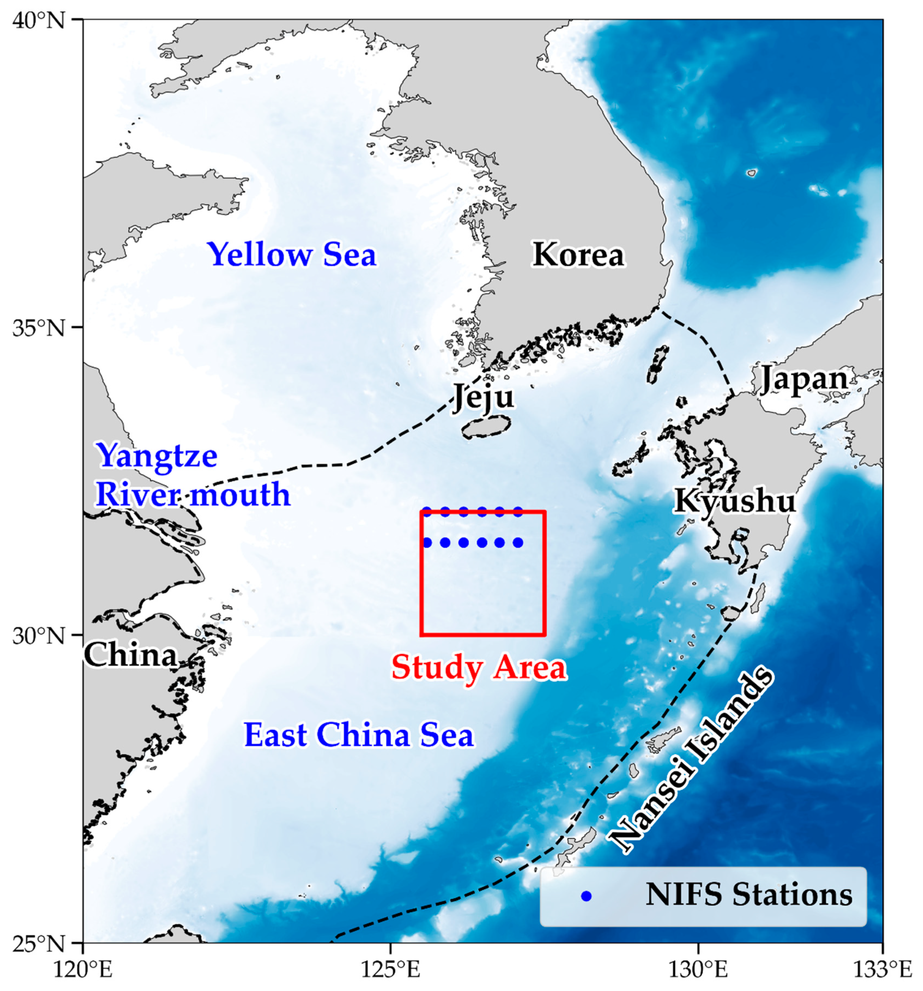
2.1. Study Area and In Situ Measurement

The study area was located in the NECS, a dynamic marginal sea bounded by the eastern coast of China, Jeju Island (off the southern coast of the Korean Peninsula), and Kyushu Island, Japan. It spans the geographical coordinates of 30–32°N and 125.5–127.5°E (Figure 1), encompassing the confluence of the Yangtze River discharge and the Kuroshio Current, representing a complex and highly variable hydrographic environment. During summer (June to September), warm, saline waters transported by a branch of the Kuroshio Current enhance surface stratification and suppress vertical mixing, fostering oligotrophic conditions that favor picophytoplankton dominance. In contrast, winter mixing increases nutrient availability, supporting the growth of larger phytoplankton such as nano- and microphytoplankton [21].

To evaluate the reliability of satellite-derived PSC estimates, we used in situ measurements of dominant PSCs collected by the National Institute of Fisheries Science (NIFS) during field surveys conducted between 2018 and 2023 at 12 stations across both coastal and offshore regions. These observations provided ground-truth data for validating satellite-based classification of phytoplankton size structure in this region.

2.2. Satellite Data and PSC Validation

This study utilized level 3 satellite data from the OC-CCI Version 6.0 (https://www.oceancolour.org/, accessed on 20 November 2024), developed by the European Space Agency (ESA). The OC-CCI dataset combines and harmonizes data from multiple ocean color sensors, offering consistent and high-quality time series of ocean color products [43]. The dataset provides global coverage with a spatial resolution of 4 km and includes key variables, such as Chl-a, the phytoplankton absorption coefficient at 443 nm (a_ph443), the diffuse attenuation coefficient at 490 nm (Kd(490)), and the remote sensing reflectance at 665 nm (Rrs665). Daily OC-CCI data were aggregated into 5-day composites to reduce noise and enhance data reliability. Satellite variables were averaged into 5-day composites using an unweighted arithmetic mean. Only cloud-free valid pixels were included, and composites were centered on each 5-day window (e.g., 1–5 January, 6–10 January, etc.). No spatial interpolation was applied. Temporal coverage of the dataset spans from 1998 to 2024, allowing for long-term trend analysis and interannual variability studies.

To validate the satellite-derived PSC estimates, in situ measurements collected within the study area by NIFS from May to September for 1998–2023 were used. Seawater samples were filtered sequentially through 20 µm and 2 µm membrane filters and a 0.7 µm GF/F filter to obtain micro-, nano-, and picophytoplankton fractions. Satellite-derived PSC estimates were derived using the semi-analytical model proposed by [45]. This model uses the inherent optical property a_ph443 to classify dominant PSCs of microphytoplankton, nanophytoplankton, and picophytoplankton. By analyzing the spectral shapes of a_ph443, the model calculates the fractional contribution of each size class to the total phytoplankton biomass. This approach is advantageous because it directly links light absorption characteristics to phytoplankton cell size, enabling more accurate PSC differentiation than provided by Chl-a-based empirical models. The relationship between a_ph443 and PSC dominance was characterized by the following general trends:

• For a_ph443 < 0.023 m⁻¹, picophytoplankton dominance;
• For a_ph443 between 0.023 and 0.069 m⁻¹, nanophytoplankton dominance;
• For a_ph443 > 0.069 m⁻¹, microphytoplankton dominance.

During summer (June to September), a_ph443 values within the study region (30–32°N, 125.5–127.5°E) ranged from 0.036 to 4.828 m⁻¹, with a mean of 0.027 m⁻¹. This range reflects strong temporal variability in phytoplankton absorption, consistent with seasonal changes in biomass and community structure.

2.3. Environmental Factors

We utilized multiple environmental datasets to analyze the key drivers of PSC variability in the NECS.

SST (°C) data were obtained from the Global Ocean Operational SST and Sea Ice Analysis (OSTIA) dataset [48], provided by the Copernicus Marine Environment Monitoring Service (CMEMS; accessed on 26 December 2024). This dataset integrates satellite observations from the Group for High-Resolution Sea Surface Temperature Project, along with in situ measurements. The OSTIA delivers daily global gap-free SST maps with a spatial resolution of 0.05° × 0.05° (~5 km), covering the temporal range from 1 January 1998 to September 2024. Reprocessed SST data were utilized for 1998–2006, whereas near-real-time SST data were employed for 2007–2024.

PAR (E/m²/d) data were obtained from the Global Merged Ocean Colour Project (GlobColour; accessed on 19 December 2024), which provides globally merged level 3 ocean color products with a spatial resolution of 4 km. The GlobColour dataset integrates observations from multiple satellite sensors, including MODIS, SeaWiFS, and MERIS, and offers consistent and validated estimates of PAR [49].

Z_eu (m) was calculated from the OC-CCI Kd(490) product, allowing for the estimation of light penetration into the water column. The relationship between Z_eu and Kd(490) follows a widely used empirical equation [27].

$$Z_{eu}(m)={\displaystyle \frac{4.6}{Kd\left(490\right)}}.$$

(1)

This equation assumes that the depth at which the PAR is reduced to 1% of its surface value corresponds to the euphotic depth.

Six-hour zonal and meridional wind data (${\mathrm{u}}_{10}$ and ${\mathrm{v}}_{10}$ m/s) were obtained from the European Centre for Medium-Range Weather Forecasts Reanalysis 5th Generation [50] dataset provided by the Copernicus Climate Data Store (accessed on 13 November 2024). Wind stress magnitude (τ, N/m²) was calculated using the bulk aerodynamic formula proposed by Large and Pond [51]. The wind stress components (τ_x and τ_y, N/m²) were first computed as follows:

$${\tau }_x(N/m^2)= {\rho }_a{C}_d{u}_{10}\sqrt{u_{10}^2+v_{10}^2},$$

(2)

$${\tau }_y(N/m^2)= {\rho }_a{C}_d{v}_{10}\sqrt{u_{10}^2+v_{10}^2},$$

(3)

where ρ_a is the air density (assumed to be 1.225 kg/m³) and C_d is the drag coefficient, determined based on wind speed following the parameterization described by Large and Pond [51].

$$C_d=0.00114+0.000076\times \left|\mathrm{U}\right|.$$

(4)

The wind stress magnitude (τ) was then calculated as the vector magnitude.

$$\tau (N/m^2)= \sqrt{{\tau }_x^2+{\tau }_y^2}.$$

(5)

These calculations were performed on 6 h data, which were then averaged to 5-day intervals for consistency with other environmental factors.

The salinity (psu) at each depth and MLD (m) was obtained from the GLORYS12V1 product, a global ocean eddy-resolving reanalysis with a horizontal resolution of 1/12° and 50 vertical levels, provided by the CMEMS (accessed on 13 December 2024).

The FWC (m) quantifies the freshwater input in a given region and is calculated based on the salinity profile relative to the reference salinity. The FWC was derived from GLORYS12V1 salinity data using the following formula [52]:

$$FWC (m)= {\int }_z^0{\displaystyle \frac{S_{ref}-S\left(z\right)}{S_{ref}}}dz,$$

(6)

where $S_{ref}$ is the reference salinity, set to 34.57 psu (Kuroshio averaged salinity) [29], and S(z) is the salinity at depth z, where z is the depth at which $\mathrm{S}=S_{ref}$.

SPM (g/m³) concentrations were estimated using the algorithm of [53] applied to the OC-CCI Rrs665 dataset, providing a measure of water clarity and sediment load. The algorithm is given by the following:

$$SPM(g/m^3)={\displaystyle \frac{A \times Rrs\left(\lambda \right)}{1-\frac{Rrs\left(\lambda \right)}{C}}},$$

(7)

where A = 17.7 and C = 0.216 for coastal waters. Rrs(λ) refers to Rrs665 (1/sr).

To ensure temporal consistency and reduce noise, all daily environmental data were aggregated into 5-day composites. Subsequently, datasets with varying native spatial resolutions were resampled to match the 4 km resolution of the OC-CCI data using the nearest-neighbors interpolation method. This approach preserves the original data characteristics by assigning the value of the closest pixel to the target grid point, facilitating the seamless integration of datasets for further analysis. Nutrient data (e.g., nitrate and phosphate) were excluded because of the inability of satellite observations to directly estimate dissolved inorganic nitrogen and phosphorus, compounded by sparse in situ spatiotemporal coverage. This exclusion may lead to the underestimation of nearshore PSC dynamics driven by the Yangtze River inputs, potentially introducing bias if riverine nutrient pulses indirectly influence physical drivers, such as Z_eu and SPM, through altered stratification or turbidity.

2.4. Statistical Analysis

To identify the environmental drivers of phytoplankton size structure, we modeled the relative contributions of each size class (pico-, nano-, and microphytoplankton) as functions of key environmental variables. Using satellite-derived data, we treated PSC contributions as dependent variables and included seven predictors—Z_eu, SST, PAR, SPM, MLD, FWC, and wind stress—in two regression frameworks: random forest and multiple linear regression. While the random forest model excelled at identifying nonlinear interactions and thresholds, multiple linear regression provided a clearer picture of the relative importance and directionality of environmental drivers under linear assumptions. Although Chl-a was initially considered as a primary dependent variable, it did not show a statistically significant relationship with the modeled PSC contributions and was therefore excluded from the final PDP visualizations.

2.4.1. Random Forest Model for PSC Analysis

A random forest algorithm was applied to evaluate the environmental drivers of PSC variability. The model, known for its ability to handle nonlinear relationships and complex interactions among variables, consists of an ensemble of decision trees, each built using a random subset of predictors and samples from the dataset. The final prediction is derived by aggregating the outputs from the individual trees [46]. In this study, the random forest model was trained and tested using a 70:30 train–test split, incorporating Z_eu and SPM as the key environmental predictors. We optimized the random forest model through grid search of key hyperparameters—parameters that control the model structure but are not learned during training—such as the number of trees and maximum tree depth. The model accuracy was assessed using root mean squared error and R² metrics. Due to its reliance on the same input data (Z_eu and SPM) in retrieval algorithms—risking the duplication of data retrieval—Chl-a was not selected as a dependent variable.

We then quantified the relative importance of key environmental variables, including SST, PAR, Z_eu, MLD, SPM, and wind stress, in influencing the contributions of pico-, nano-, and microphytoplankton. Partial dependence plots (PDPs) were generated to visualize and interpret the influence of individual environmental variables on PSCs. PDPs illustrate the marginal effect of a selected predictor variable on PSCs while holding other variables constant. These plots provide insights into the relationships between specific environmental factors. They reveal critical thresholds or inflection points, aiding in understanding the nonlinear and interactive effects captured by the random forest model.

2.4.2. Multiple Linear Regression Analysis for PSCs

Multiple linear regression analysis was conducted to explore the relationship between environmental variables (e.g., Z_eu, SPM, SST, PAR, wind stress, and FWC) and dependent variables, such as PSCs. This statistical method assumes a linear relationship between the predictor and response variables, enabling the identification of significant environmental drivers. The regression model was validated by assessing key metrics, including adjusted R², p-values, and the variance inflation factor, to detect multicollinearity. The prediction equation for the model is as follows:

$$\begin{gathered} Contribution (\%) ={\beta }_0+ {\beta }_1\times SST+{\beta }_2\times FWC+ {\beta }_3\times MLD+ {\beta }_4\times Wind stress+ {\beta }_5\times PAR+ \\ {\beta }_6\times Z_{eu}+ {\beta }_7\times SPM. \end{gathered}$$

(8)

2.5. MHW Definition and Detection

We examined the occurrence of MHWs, defined as discrete, prolonged periods of anomalously high SSTs relative to the local climatological mean. Specifically, we defined an MHW as any period when the 5-day averaged SST exceeded the 90th-percentile threshold for at least two consecutive intervals (for a total of 10 days). This method was adapted from [39] to match the temporal resolution of our satellite-based 5-day composite SST data. The 90th-percentile threshold was calculated for the entire dataset (1998–2024). This approach ensured that the persistence criterion aligned with the temporal resolution of the dataset, thereby avoiding spurious detections of isolated high-temperature events. Data for MHW periods were compared with those for non-MHW periods to assess their impact on environmental variables.

3. Results

3.1. Validation of the PSC Models

Size-fractionated in situ dominant PSC data (2018–2023) confirmed an accuracy of 69.8% for the satellite-derived dominant PSCs (

Table 1. Validation results of satellite-derived dominant PSCs (model of [45]) against in situ PSCs (2018–2023). Mismatched dominant PSCs are in italics.

Date (yyyy-mm-dd)	Latitude	Longitude	In Situ Dominant PSC	Satellite Dominant PSC
2018-05-04	32.000	126.505	Pico	Pico
2018-05-04	31.989	126.516	Pico	Pico
2018-05-04	32.003	125.889	Nano	Pico
2019-05-10	31.499	125.906	Pico	Pico
2019-05-10	31.493	125.879	Nano	Pico
2019-05-09	31.998	127.068	Pico	Pico
2019-05-08	32.000	126.486	Micro	Pico
2019-05-08	31.998	126.484	Pico	Pico
2019-05-08	31.498	126.492	Pico	Pico
2022-05-18	31.498	125.893	Pico	Nano
2022-05-18	32.000	127.072	Pico	Pico
2022-05-16	32.009	126.456	Micro	Pico
2022-05-16	31.997	125.885	Micro	Pico
2022-05-17	31.498	126.492	Pico	Pico
2023-05-02	32.012	125.887	Pico	Nano
2023-05-10	31.500	126.485	Pico	Pico
2023-05-02	31.500	126.495	Pico	Pico
2023-05-02	31.998	126.484	Pico	Pico
2018-08-06	32.007	125.895	Pico	Nano
2018-08-06	31.994	125.884	Nano	Nano
2018-08-05	31.502	127.072	Pico	Pico
2018-08-04	31.500	126.494	Pico	Pico
2018-08-04	31.501	126.492	Pico	Pico
2020-08-14	31.508	126.510	Pico	Nano
2020-08-14	31.485	126.489	Pico	Pico
2020-08-14	31.501	125.888	Pico	Pico
2020-08-15	32.000	127.071	Pico	Pico
2020-08-15	32.000	127.070	Pico	Pico
2020-08-15	31.504	127.070	Pico	Pico
2021-08-28	32.000	125.888	Micro	Nano
2021-08-28	31.970	125.909	Pico	Nano
2021-08-28	31.502	127.014	Pico	Pico
2021-08-31	31.998	126.484	Nano	Nano
2022-08-22	32.003	127.076	Pico	Pico
2022-08-22	32.000	127.082	Pico	Pico
2022-08-23	31.498	126.492	Micro	Pico
2022-08-23	31.500	125.892	Pico	Pico
2023-08-28	31.505	127.077	Pico	Pico
2023-08-27	31.499	126.494	Pico	Pico
2023-08-27	31.501	125.885	Nano	Pico
2023-08-26	31.500	125.892	Pico	Pico
2023-08-26	31.997	125.885	Pico	Pico
2023-08-26	31.504	127.070	Pico	Pico
30/43 (69.8%) of matched pixels

). The discrepancies are likely due to optical ambiguity in mixed communities and intermediate SPM conditions. Most mismatches occurred in the northwestern region of the study area, suggesting that coastal or turbid waters near the Yangtze River plume may contribute to classification uncertainty in PSC estimation. Only data in which the dominant PSC represented more than 10% of the valid data of the total pixels (1585 of 1860 valid data) within the study area were included in the analysis.

The contribution of each PSC was calculated as a regional average, representing the proportion of pixels within the study area where each size class was dominant.

3.2. Phytoplankton Dynamics During the Summer Season

From June to September (1998–2024), each biological and environmental factor showed distinct temporal variability (Figure 2) based on the mid-day average of each 5-day period. However, for variables such as Chl-a, SPM, Z_eu, and wind stress, the differences between climatological means—such as between Chl-a values on 7 June and 5 September—remained within the range of standard deviations, indicating a lack of statistically significant variation during the summer season. Figure 2a illustrates the consistently high contribution of picophytoplankton, ranging from 59.4% to 86.5% with an average of 70.2% (±7.6%), indicating their dominant role. Climatologically, the picophytoplankton contribution peaked on 17 June (86.5%) and declined to 59.4% by 1–6 August, after which it increased slightly. The nanophytoplankton contribution exhibited a complementary pattern to the picophytoplankton contribution, playing a secondary role in the community structure and reaching a minimum of 13.5% on 17 June. Subsequently, the nanophytoplankton proportion steadily increased, peaking at 38.2% on 27 July with an overall average contribution of 28.8% (±6.6%). The nanophytoplankton contribution fluctuated in tandem with the declining picophytoplankton dominance. Microphytoplankton had the lowest contribution, averaging 2.0% (±1.9%) and ranging from 0.02% to 6.6%. These larger phytoplankton, which are often reliant on nutrient-rich and turbulent conditions, are less competitive in the observed stratified and nutrient-limited environment [54].

The Chl-a concentration over the study period ranged from 0.17 to 2.15 mg/m³, with an average value of 0.55 ± 0.28 mg/m³. Previous studies have reported Chl-a concentrations in the ECS ranging from 0.02 to 6.19 mg/m³, depending on location, season, and influencing factors [21,29,55]. Notably, [55] observed Chl-a concentrations ranging from 0.02 to 2.5 mg/m³ in the shallower Kuroshio-influenced area, closely aligning with the values recorded in this study. The picophytoplankton contribution ranged from 0% to 100%, averaging 69.5% ± 26.3%; nanophytoplankton from 0% to 94.0%, averaging 28.3% ± 23.5%; and microphytoplankton from 0% to 62.4%, averaging 2.2% ± 7.0%. Seasonal changes in PSCs appear to be influenced by the intrusion of the Kuroshio Current, which brings warm, oligotrophic waters into the NECS. These waters are characterized by high temperature and salinity but low nutrient concentrations, potentially suppressing vertical nutrient fluxes due to thermal stratification and supporting smaller phytoplankton groups, such as picophytoplankton [56].

3.3. Fluctuation of Environmental Variables During the Summer Season

In this study, the analyzed environmental variables derived from climatological data included SST, Z_eu, SPM, MLD, PAR, FWC, and wind stress (Figure 2c–i). These variables were evaluated to understand temporal climate variability during the study period. All environmental and biological variables analyzed in this study—including SST, Z_eu, SPM, MLD, PAR, FWC, wind stress, and Chl-a concentration—exhibited statistically significant temporal variability across months (p < 0.05 for all, Kruskal–Wallis test). SST showed a mean value of 26.24 ± 2.64 °C, with a range from 20.57 to 29.03 °C. Z_eu averaged 80.86 ± 4.32 m, with values ranging from 75.10 to 90.83 m. Average SPM concentrations were 0.0021 ± 0.00035 g/m³, with a range of 0.0015 to 0.0028 g/m³. MLD averaged 14.29 ± 5.34 m, with a range from 10.55 to 27.28 m. PAR values were 44.09 ± 5.70 E/m²/d on average, ranging from 33.95 to 52.76 E/m²/d. FWC had a mean value of 2.11 ± 0.51 m, ranging from 1.49 to 2.87 m. Finally, wind stress averaged 0.0072 ± 0.0014 N/m², ranging from 0.0042 to 0.0092 N/m². These factors collectively define light and nutrient conditions, thereby influencing phytoplankton community structure.

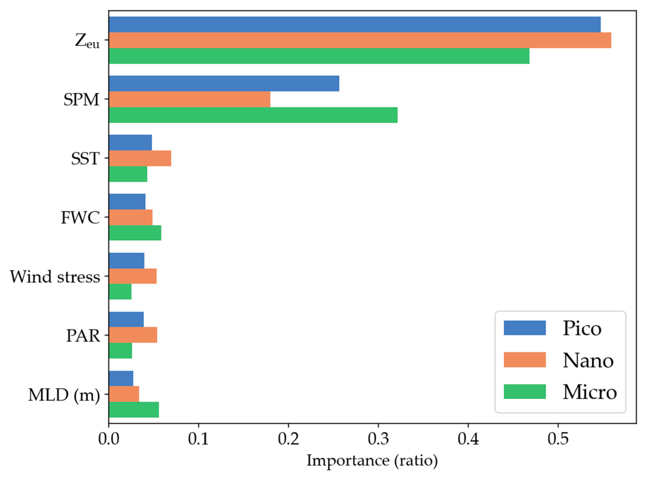
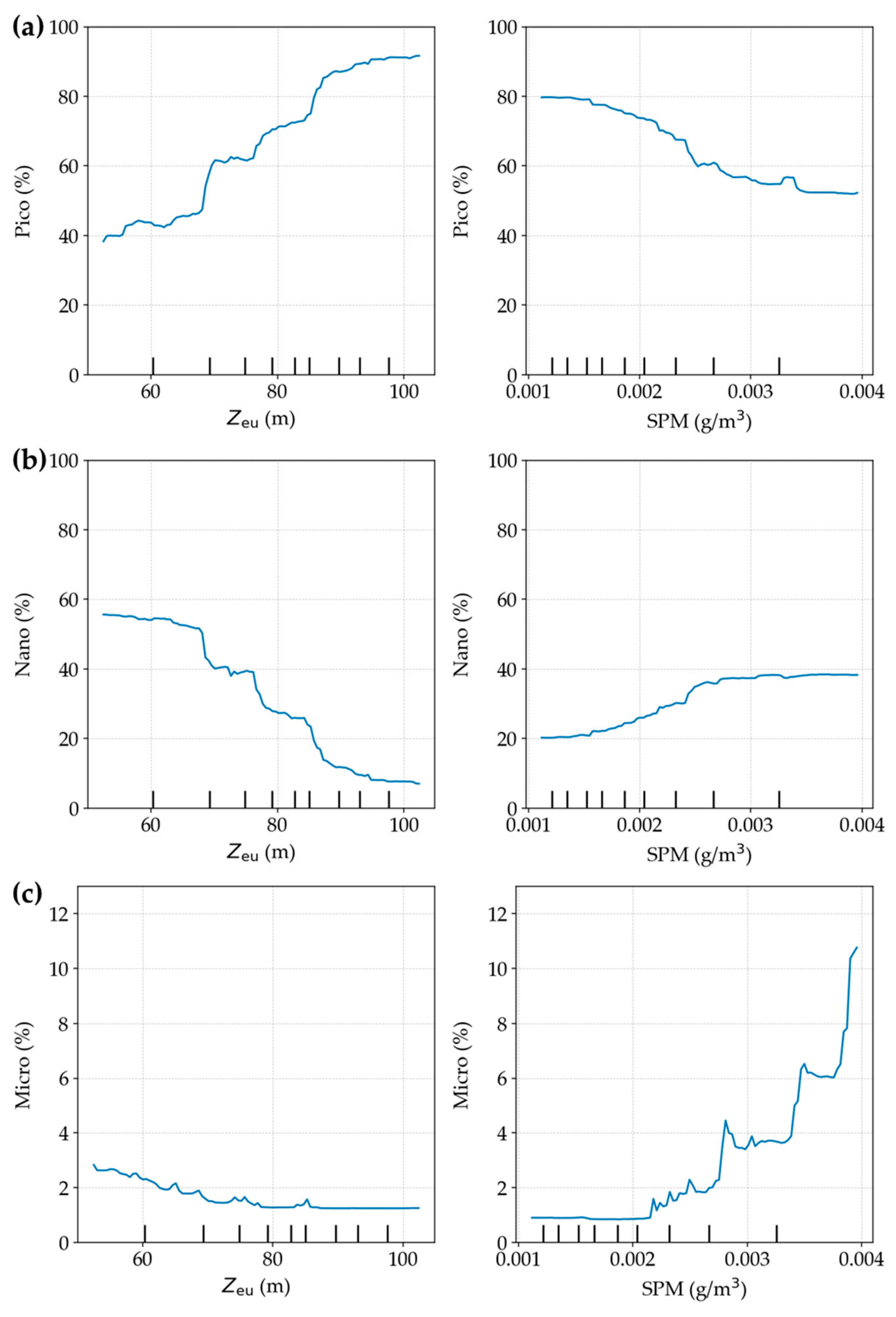
3.4. Major Driving Factors of PSC Variability

The analysis using random forest showed that Z_eu and SPM explained a substantial proportion of the variability in PSC contributions (Figure 3). All predictor variables used in the random forest and multiple regression exhibited statistically significant monthly differences (p < 0.05 for all; Kruskal–Wallis test), justifying their inclusion in the temporal modeling of PSC variability. The picophytoplankton contribution increased sharply with Z_eu, particularly beyond a value of 70 m, as confirmed by the PDP (Figure 4a). In contrast, SPM was associated with significantly reduced contributions beyond 0.0025 g/m³, indicating that SPM limited the dominance of smaller phytoplankton (Figure 4a). Conversely, the contribution of picophytoplankton declined when SPM exceeded 0.0025 g/m³, indicating that higher SPM may hinder the growth of smaller cells.

Regarding the nanophytoplankton contribution, the analysis demonstrated a strong negative correlation with Z_eu. As shown in the PDP (Figure 4b), nanophytoplankton contributions decreased markedly as Z_eu increased beyond 60 m. However, SPM exhibited a mildly positive relationship with the contribution of the PSC, suggesting that nano-sized phytoplankton may have an adaptive advantage in turbid environments with more particulate matter.

The microphytoplankton contribution showed a distinct pattern compared with those of the smaller size classes. Their contribution remained relatively stable across varying Z_eu levels, as illustrated in the PDP (Figure 4c), but increased substantially when SPM levels exceeded 0.003 g/m³. This indicates that higher particle loads may favor larger phytoplankton classes, possibly because of their ability to utilize particulate organic matter as a resource or to adapt to lower light conditions.

The multiple regression results are presented in Figure 5 and

Table 2. Multiple linear regression results for each PSC.

Pico	Coef. (βi)	Std. Err.	t	p > |t|
Const.	0.0000	0.0233	0.0000	1.0000
SST	0.0837	0.0319	2.6264	0.0089
FWC	0.1924	0.0348	5.5252	0.0000
MLD	0.0941	0.0319	2.9442	0.0034
Wind stress	−0.0955	0.0245	−3.9065	0.0001
PAR	−0.0763	0.0290	−2.6292	0.0088
Zeu	0.6494	0.0326	19.8920	0.0000
SPM	−0.1985	0.0336	−5.9006	0.0000
Nano	Coef. (βi)	Std. Err.	t	p > |t|
Const.	0.0000	0.0272	0.0000	1.0000
SST	−0.1010	0.0372	−2.7181	0.0068
FWC	−0.1743	0.0406	−4.2915	0.0000
MLD	−0.0236	0.0373	−0.6336	0.5266
Wind stress	0.0849	0.0285	2.9782	0.0030
PAR	0.0985	0.0338	2.9115	0.0037
Zeu	−0.6891	0.0381	−18.1003	0.0000
SPM	0.0613	0.0392	1.5625	0.1187
Micro	Coef. (βi)	Std. Err.	t	p > |t|
Const.	0.0000	0.0308	0.0000	1.0000
SST	0.0242	0.0421	0.5739	0.5663
FWC	−0.1388	0.0460	−3.0151	0.0027
MLD	−0.2744	0.0422	−6.5001	0.0000
Wind stress	0.0742	0.0323	2.2978	0.0219
PAR	−0.0437	0.0384	−1.1386	0.2554
Zeu	−0.1299	0.0431	−3.0116	0.0027
SPM	0.5407	0.0445	12.1608	0.0000

. The model explained the picophytoplankton contribution well (Figure 5, Table 2). The picophytoplankton contribution was well predicted, with R² = 0.686 (Figure 5a). The key factors influencing model prediction, based on t-values, were Z_eu, SPM, and FWC (Table 2). Similarly, the nanophytoplankton contribution showed a moderate level of predictability, with R² = 0.573 (Figure 5b). Influential variables for the nanophytoplankton contribution included Z_eu and FWC, which were highlighted as factors significantly affecting the model’s accuracy (Table 2). In contrast, the microphytoplankton contribution had a relatively low R² value of 0.452 (Figure 5c), indicating that the model struggled to accurately predict these contributions (Table 2). ${\beta }_i$ represents the coefficient of each environmental factor.

Comparison of Random Forest and Multiple Linear Regression Results

The analysis results of random forest captured a nonlinear threshold where the picophytoplankton contribution surged beyond a Z_eu of 70 m (Figure 4a), whereas multiple linear regression emphasized a linear Z_eu effect (R² = 0.686), missing such thresholds. This suggests that nonlinear interactions are critical for PSC variability. Overall, the random forest model outperformed multiple linear regression in predictive performance, with higher R² values for pico- and nanophytoplankton (0.69 and 0.57, respectively) compared to 0.53 and 0.41 in the regression model. In addition to capturing nonlinear threshold responses, such as the sharp decline in pico dominance at elevated SPM levels, the random forest approach provided robust variable importance measures. In contrast, the regression model offered interpretability through standardized coefficients and p-values, enabling mechanistic insights under linear assumptions. These complementary strengths suggest that combining both approaches enhances our understanding of PSC-environment relationships.

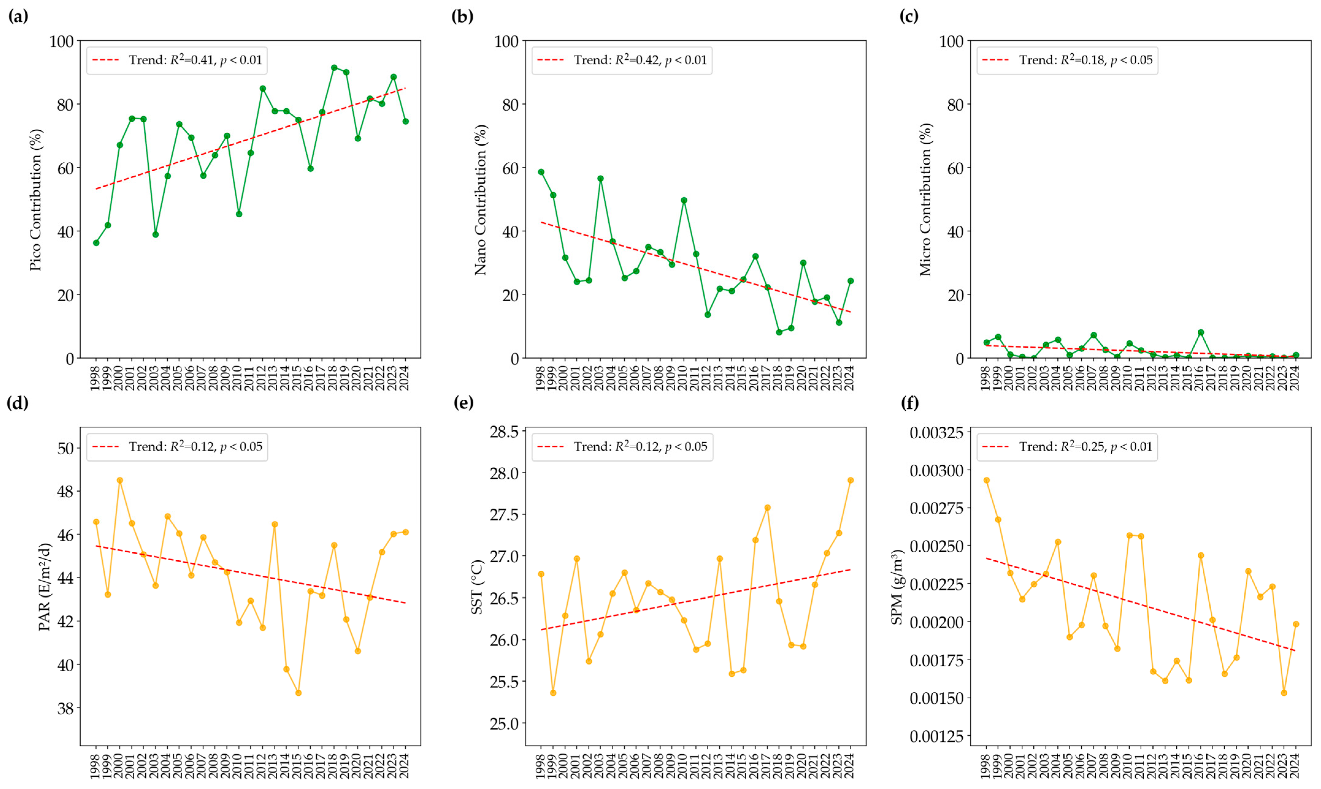
3.5. Decadal Changes in PSCs and Key Environmental Factors in the Summer

In Figure 6, each data point represents the spatial and temporal mean for the summer period (June to September) of a given year. Specifically, values were averaged across all grid cells in the study area and all time points within that seasonal window. Summer data (June–September) revealed statistically significant trends in PSC contributions and key environmental variables from 1998 to 2023. The picophytoplankton contribution exhibited an annual increase of 2.4% (p < 0.01), indicating a shift toward smaller phytoplankton during the study period (

Table 3. Annual changes in environmental factors and PSC contributions.

Variable	Slope	Significance (p-Value)	Annual Change (%)	Trend
Pico (%)	0.0032	<0.01	+2.4	Increasing
Nano (%)	−0.0029	<0.01	−2.2	Decreasing
Micro (%)	−0.0004	<0.01	−0.4	Decreasing
Chl-a (mg/m3)	0.0000	≥0.05
PAR (E/m2/d)	−0.0003	<0.05	−0.3	Decreasing
SST (°C)	0.0001	<0.05	+0.1	Increasing
Zeu (m)	0.0004	≥0.05
FWC (m)	0.0000	≥0.05
MLD (m)	0.0001	≥0.05
Wind stress (N/m2)	0.0000	≥0.05
SPM (g/m3)	0.0000	<0.01	−0.3	Decreasing

, Figure 6). In contrast, the nano- and microphytoplankton contributions showed annual decreases of 2.2% (p < 0.01) and 0.4% (p < 0.01), respectively, during the study period. The decadal variation in PSCs in the summer had no statistically significant association with Chl-a concentrations, suggesting stable total phytoplankton biomass despite shifts in PSC composition. The PAR decreased at a rate of 0.3% per year (p < 0.05), reflecting a potential reduction in light availability during summer. The slopes and p-values indicated that these trends were statistically robust (Table 3). These results indicate that the variability in PSCs is closely related to light availability and water turbidity, as represented by Z_eu and SPM. SPM, which showed a negative correlation with the picophytoplankton contribution in the previous section, also exhibited a decreasing trend (Table 3, Figure 6), which likely played a critical role in the observed increase in picophytoplankton contribution.

3.6. Biological Responses to MHWs and Environmental Differences

MHWs induced significant changes in biological and environmental variables within the study region. We identified four MHW periods: (1) 29 August–8 September 2017, (2) 24 August–2 September 2022, (3) 3 September–2 October 2023, and (4) 28 August–1 October 2024. When reporting changes in variables, we primarily used relative increases. During MHW events, the picophytoplankton contribution increased by 41.2% relative to the baseline value (from 65.0% to 91.7%), equivalent to a 1.41-fold increase (

Table 4. Differences in biological and environmental factors between MHW and non-HMW periods. The p-values were calculated by Mann–Whitney U. “n.s.” indicates not significant (p ≥ 0.05).

Variables	Non-MHW Periods	MHW Periods	Relative Increase (%)	Significance
Pico	65.0 ± 27.2%	91.7 ± 15.2%	41.2%	p < 0.01
Nano	31.7 ± 23.3%	7.8 ± 14.1%	−75.2%	p < 0.01
Micro	3.4 ± 8.6%	0.4 ± 1.4%	−87.5%	p < 0.01
Chl-a	0.60 ± 0.33 mg/m3	0.32 ± 0.13 mg/m3	−46.5%	p < 0.01
PAR	42.78 ± 8.95 E/m2/d	43.39 ± 6.0 E/m2/d	1.4%	p < 0.01
SST	27.89 ± 1.34 °C	29.20 ± 0.71 °C	4.7%	p < 0.01
Zeu	77.74 ± 15.67 m	98.26 ± 11.88 m	26.4%	p < 0.01
FWC	1.65 ± 0.4 m	1.59 ± 0.23 m	−3.9%	n.s.
MLD	18.04 ± 6.94 m	19.4 ± 3.87 m	7.6%	n.s.
Wind stress	0.0076 ± 0.0036 N/m2	0.0072 ± 0.0034 N/m2	−4.8%	n.s.
SPM	0.0024 ± 0.0012 g/m3	0.0016 ± 0.0001 g/m3	−35.4%	n.s.

). Statistically significant differences between MHW and non-MHW conditions were observed for most biological and environmental variables, including Z_eu, SST, SPM, and all PSC components (p < 0.01; Mann–Whitney U test), while PAR, wind stress, and FWC showed no significant difference. The nanophytoplankton and microphytoplankton contributions experienced significant reductions of 75.2% and 87.5%, respectively. The mean Chl-a concentration decreased by approximately 46.5%, dropping from 0.60 mg/m³ under non-MHW conditions to 0.32 mg/m³. The mean SST during MHW periods was 29.2 °C, compared to 27.89 °C under non-MHW conditions. Z_eu and SPM exhibited the most significant changes among all environmental variables, increasing by 26.4% and decreasing by 35.4%, respectively. The MLD increased by 7.6%, whereas the PAR and wind stress remained relatively stable, with minor changes of 1.4% and −4.8%, respectively (Table 4).

Because Z_eu and SPM exhibited the largest relative changes during MHW events, they were likely the key environmental factors driving the observed shifts in chl-a and PSC distributions under these conditions. These results highlight the distinct shifts in phytoplankton community composition and Chl-a concentration in response to MHWs, indicating potential ecosystem-level effects. Such effects may include reduced primary productivity, disruption of energy transfer to higher trophic levels, and altered biogeochemical cycling.

4. Discussion

4.1. PSC Variability and Key Environmental Drivers

Although month-to-month changes in Z_eu and SPM during summer were sometimes within the range of standard deviations (Section 3.2), both variables exhibited statistically significant long-term trends over the 27-year period (Table 3). These long-term shifts justify their role as key drivers in the observed restructuring of PSCs, particularly when analyzed using threshold-sensitive models, such as random forest. This study highlights Z_eu and SPM as critical environmental drivers shaping PSC variability in the NECS during summer using two statistical methods (Section 3.4). Although both the random forest and multiple linear regression analyses identified Z_eu and SPM as the primary drivers of PSC variability, the two methods revealed complementary insights, with random forest capturing abrupt shifts in PSC dominance under specific conditions. Random forest modeling highlighted nonlinear threshold effects, such as the sharp decline in picophytoplankton contribution when SPM exceeded 0.0025 g/m³ (Figure 4a). In contrast, multiple linear regression assumed linear relationships and thus underestimated the impact of such thresholds (Table 2). The higher R² values for the random forest results suggest that nonlinear interactions play an important role in PSC dynamics. This discrepancy underscores the importance of using complementary methods to capture both linear trends and complex ecological interactions [47,57]. Regression modeling effectively quantified the linear contributions of key variables, such as Z_eu and SPM, but may have overlooked the complex interactions between them. These results suggest that the choice of statistical approach can influence the interpretation of environmental drivers, underscoring the complementary strengths of both methods.

Our analysis of 27 years of data revealed detailed mechanistic links between Z_eu and SPM. Variations in SPM concentrations, driven by monsoonal shifts and riverine discharge, modulate Z_eu by affecting light penetration, which is essential for phytoplankton photosynthesis and productivity [58,59]. This dynamic interaction creates heterogeneous light environments that shape phytoplankton growth and PSC composition across seasons [23]. Increased SPM reduces Z_eu by scattering and absorbing light, creating turbid conditions that favor nano- and microphytoplankton in nearshore areas [60]. Conversely, lower offshore SPM concentrations enhance light availability, allowing picophytoplankton to dominate when light penetration exceeds 70 m [15,27]. SPM-induced turbidity reduces light availability in the water column, favoring phytoplankton that can tolerate low-light conditions. Microphytoplankton, owing to their higher pigment content and adaptive strategies, face more competition than smaller picophytoplankton under such conditions [24,60]. While our SPM data do not distinguish between organic (particulate organic matter; POM) and inorganic (particulate inorganic matter; PIM) particles, studies have shown that PIM dominates SPM composition in the NECS, particularly near the Yangtze River plume during high discharge or resuspension events [23,27]. As PIM is more effective at scattering light, this supports the use of SPM as a proxy for turbidity and optical limitation. This may explain why SPM, rather than Chl-a, showed a stronger association with PSC variability in our model [61,62]. These findings align with those of previous studies, demonstrating the critical role of light conditions in regulating phytoplankton community composition. Previous studies have suggested that nutrients adsorbed onto SPM may be released into the water column, potentially providing an additional source of bioavailable nutrients for phytoplankton growth, which warrants further investigation in the ECS [63,64]. Such nutrient dynamics are particularly beneficial for larger cells such as microphytoplankton, which possess higher uptake capacities under nutrient-rich conditions [65]. While nutrient availability supports microphytoplankton, such as diatoms in nutrient-rich nearshore waters [19,30], in offshore areas, where nutrient inputs are lower, physical factors, such as Z_eu and SPM, may exert a greater influence on PSC variability. Future research integrating nutrient profiles, including N/P ratios and dissolved organic matter, will help clarify the complex interactions between the physical and biogeochemical drivers of phytoplankton dynamics. For example, [22] demonstrated that N/P ratios exceeding 16:1 reduced picophytoplankton competitiveness, offering a pathway to address the nutrient data gap in this study. In addition to nutrient and light dynamics, SPM may directly affect smaller phytoplankton through physical interactions, such as sinking or aggregation, which reduces their ability to remain in the photic zone [66,67]. These combined effects suggest that elevated SPM concentrations can shift the community dominance from pico- to microphytoplankton, particularly in environments with high nutrient availability and low-light conditions.

As a proxy for riverine freshwater input, particularly from the Yangtze River, FWC emerged as an influential factor, particularly in the multiple regression analysis. FWC can modify salinity and stratification, thereby influencing phytoplankton dynamics through changes in nutrient availability and water column structure [19,21,59]. Lower FWC values, indicative of weaker freshwater input, may reduce stratification, enhance nutrient mixing, and support larger phytoplankton, such as microphytoplankton. Conversely, higher FWC values, often associated with surface stratification, can limit nutrient flux to the euphotic zone, favoring picophytoplankton dominance. These findings highlight the dual role of FWC in modulating both physical and biogeochemical conditions in the NECS. The considerable influence of FWC in the regression models suggests that it may mediate PSC variability through stratification and nutrient dynamics, which requires further investigation using nutrient data. The Kuroshio Current, which transports warm oligotrophic waters into the ECS, may further contribute to stratification and nutrient limitation, promoting picophytoplankton dominance in offshore regions [18,38,56].

Notably, the model used for multiple regression exhibited a relatively low R² value for microphytoplankton contributions, suggesting that the linear model might not fully capture the dynamics governing this PSC. This discrepancy implies that microphytoplankton contributions may be influenced by additional factors—such as episodic nutrient pulses, grazing dynamics, and physical-biological coupling processes (e.g., eddy-like structures) that enhance nutrient supply—which were not accounted for by the physical variables included in our analysis [30,65,68]. Moreover, the emergence of FWC as a key factor affecting pico- and nanophytoplankton underscores the complexity of ecological interactions in the NECS. Future studies should consider incorporating additional biogeochemical and ecological variables to better model microphytoplankton dynamics. While the PSC model shows limited pixel-level accuracy, its performance is sufficient for detecting regional-scale trends in phytoplankton size structure. This justifies its use in examining seasonal patterns and MHW-induced changes, although localized misclassifications may introduce uncertainty in finer-scale interpretations.

4.2. Long-Term Trends in PSC Dynamics in the NECS During Summer and Their Implications

Over the 27-year study period, clear long-term trends were observed in PSC composition. Picophytoplankton contributions increased annually by 2.4%, whereas nano- and microphytoplankton contributions decreased by 2.2% and 0.4%, respectively (Table 3, Figure 6). These findings are consistent with global patterns of phytoplankton community restructuring under climate change [15,69]. Rising SSTs driven by anthropogenic climate change [70] represent a key factor favoring smaller phytoplankton. Picophytoplankton, with their high surface area-to-volume ratios, thrive in warm oligotrophic environments [6]. Additionally, the observed decline in SPM concentrations (Figure 6f) was associated with increased Z_eu, further promoting picophytoplankton growth in offshore areas where light penetration exceeded 70 m. Larger phytoplankton, such as diatoms and dinoflagellates, are less competitive under these conditions because they require higher nutrient availability and often thrive in turbulent, nutrient-rich environments.

The observed shift toward picophytoplankton dominance has far-reaching ecological and biogeochemical consequences. An increased dominance of smaller phytoplankton intensifies the microbial loop, reducing energy transfer efficiency to higher trophic levels, including fish and marine mammals [6,17]. This shift can lead to potential declines in fishery productivity [71], with significant socioeconomic implications for the region. Such disruptions are particularly critical in the ECS, a region where fisheries depend heavily on trophic level stability to sustain marine resources [10,69]. The dominance of smaller phytoplankton reduces the availability of energy-rich diatoms and large phytoplankton, which form the foundation of fishery productivity, thereby exacerbating the vulnerability of higher trophic levels to climate-induced stressors [6]. In addition, smaller phytoplankton contribute less to the biological carbon pump, resulting in reduced carbon export to the deep ocean and altered nutrient cycling in benthic ecosystems [10,44]. This reduced carbon export efficiency is particularly concerning in regions, such as the ECS, where the decline in diatoms, a major contributor to silica cycling, may disrupt the balance between carbon and silicon biogeochemistry [72]. Furthermore, the replacement of diatoms by smaller phytoplankton groups could limit silica deposition in benthic systems, thereby affecting benthic ecosystems that are reliant on diatomaceous sediments [73].

The shift toward picophytoplankton dominance and its cascading effects emphasize the need for adaptive management strategies to mitigate the effects of climate change on marine ecosystems in the ECS. However, these trends vary across marginal seas owing to differing environmental conditions. Unlike the nutrient-rich Yellow Sea, where microphytoplankton persist despite rising SSTs due to ample nutrient inputs [74], the oligotrophic NECS shows picophytoplankton dominance, similar to patterns in the South China Sea and subtropical North Pacific under climate change [15]. These regional differences are driven by the ECS’s unique combination of Yangtze River nutrient inputs and Kuroshio Current oligotrophy, which amplifies the effects of rising SSTs and MHWs on PSC shifts. Developing adaptive management strategies requires the integration of long-term satellite observations with high-resolution in situ measurements to monitor phytoplankton community shifts [75]. Predictive ecosystem models that incorporate physical, chemical, and biological variables can aid in anticipating the cascading effects of community shifts and inform sustainable fishery management practices [69,70].

Analysis results regarding MHWs further amplify these long-term trends. MHWs, characterized by anomalously long periods of elevated SSTs, have become more frequent, lengthy, and intense in recent decades owing to climate change [39,40]. Our results indicate that during MHW events, defined according to [39] as periods when SSTs exceed the 90th percentile (i.e., unusually warm relative to the local seasonal climatology) for at least two consecutive intervals, the alteration in light penetration and nutrient mixing leads to a marked shift in PSC distributions, notably favoring picophytoplankton. MHWs intensify water column stratification, further reducing nutrient flux into the euphotic zone and favoring picophytoplankton dominance while suppressing larger phytoplankton. Stratification intensifies during MHW events, further limiting nutrient mixing in the euphotic zone. Picophytoplankton contributions increased sharply (65.0 ± 27.2% to 91.7 ± 15.2%) during MHWs, whereas nano- and microphytoplankton contributions declined by 75.2% (31.7 ± 23.3% to 7.8 ± 14.1%) and 87.5% (3.4 ± 8.6% to 0.4 ± 1.4%), respectively (Table 4). These results align with the finding that thermal anomalies disproportionately favor smaller phytoplankton that are better adapted to nutrient-poor conditions [41]. The combined effects of rising SSTs, declining SPM, and episodic MHWs create feedback loops that reinforce the dominance of smaller phytoplankton in the NECS. The observed increases in picophytoplankton due to declining SPM, deepening Z_eu, and intensifying MHWs are strongly influenced by the Kuroshio Current. This western boundary current stabilizes ECS offshore regions by transporting warm oligotrophic waters, enhancing stratification, and limiting nutrient mixing. During MHWs, the Kuroshio warming effect is amplified, further intensifying nutrient limitations in the euphotic zone and favoring picophytoplankton dominance under these conditions [18,38,59]. Moreover, the Kuroshio Current-induced suppression of SPM dispersion from coastal and riverine sources reduces turbidity, leading to greater Z_eu and a more favorable light environment for smaller phytoplankton [27,59]. This shift toward smaller phytoplankton size in the composition has important implications for marine ecosystems, as it disrupts traditional food webs and reduces ecosystem resilience.

4.3. Study Limitations and Future Directions

The results of our analysis offer valuable insights into PSC variability; it has some limitations that warrant further investigation. Although validated, reliance on satellite-derived data introduces potential biases, particularly in coastal regions where atmospheric corrections are more challenging. Expanding in situ validation efforts will improve the accuracy of PSC estimates. Furthermore, this study focused on summer conditions; however, PSC dynamics may differ in other seasons because of variations in nutrient availability, hydrography, and light conditions. Expanding the temporal scope to include spring, autumn, and winter would provide a more comprehensive understanding of PSC variability.

This study identified Z_eu and the SPM as the primary drivers of PSC variability in the NECS. However, analyzing seasonal variations in N/P ratios and their influence on phytoplankton productivity could provide deeper insights. For example, fluctuations in N/P ratios may limit picophytoplankton growth or enhance the competitiveness of larger phytoplankton in nutrient-enriched regions [19,30]. Future research should explore the interactions between physical drivers (e.g., stratification and wind stress) and biogeochemical factors (e.g., nutrient fluxes and grazing pressure). Long-term ecosystem monitoring and modeling are critical for predicting and mitigating the impacts of climate change on the NECS.

5. Conclusions

The northern East China Sea (NECS) plays a vital role in supporting regional fisheries, maintaining biodiversity, and supporting the global carbon cycle. Recent advances in remote sensing have allowed for the large-scale monitoring of PSC distributions in this region, offering new opportunities to explore the links between phytoplankton diversity, productivity, and ecosystem health. The long-term monitoring of this dynamic ecosystem is essential for identifying critical thresholds and predicting future changes under the combined pressures of climate change and human activity. Early warning signals of ecosystem stress can inform adaptive management strategies and ensure the sustainability of marine resources and ecosystem services in economically and ecologically significant regions.

In this study, we demonstrated that over a 27-year period, the summer phytoplankton community in the NECS has undergone considerable restructuring, with picophytoplankton contributions increasing by approximately 2.4% per year, whereas nano- and microphytoplankton contributions have declined. Our analysis revealed that changes in Z_eu and SPM were the primary environmental drivers of these shifts. Specifically, deeper Z_eu values favor the proliferation of picophytoplankton, whereas higher SPM levels tend to support larger phytoplankton groups. Additionally, MHW events exacerbate these trends by intensifying water column stratification and limiting nutrient availability, further promoting picophytoplankton dominance. These alterations in the phytoplankton community structure are likely to reduce trophic transfer efficiency and carbon export, with potential long-term consequences for regional fisheries and ecosystem stability. Given the exclusion of nutrient data due to current limitations, future studies should integrate high-resolution nutrient measurements to comprehensively assess the interplay between physical and biogeochemical drivers. Ultimately, our findings highlight the critical need for sustained monitoring and adaptive management strategies to mitigate the impact of climate change on dynamic NECS ecosystems.

References

1. Field, C.B.; Behrenfeld, M.J.; Randerson, J.T.; Falkowski, P. Primary production of the biosphere: Integrating terrestrial and oceanic components. Science 1998, 281, 237–240. [Google Scholar] [CrossRef]
2. Agawin, N.S.R.; Duarte, C.M.; Agustí, S. Nutrient and temperature control of the contribution of picoplankton to phytoplankton biomass and production (Errata). Limnol. Oceanogr. 2000, 45, 591–600. [Google Scholar] [CrossRef]
3. Platt, T.; Jassby, A.D. The Relationship between Photosynthesis and Light for Natural Assemblages of Coastal Marine Phytoplankton. J. Phycol. 1976, 12, 421–430. [Google Scholar] [CrossRef]
4. Sigman, D.M.; Hain, M.P. The biological productivity of the ocean. Nat. Educ. Knowl. 2012, 3, 21. [Google Scholar]
5. Bar-On, Y.M.; Phillips, R.; Milo, R. The biomass distribution on earth. Proc. Natl. Acad. Sci. USA 2018, 115, 6506–6511. [Google Scholar] [CrossRef]
6. Behrenfeld, M.J.; O’Malley, R.T.; Siegel, D.A.; McClain, C.R.; Sarmiento, J.L.; Feldman, G.C.; Milligan, A.J.; Falkowski, P.G.; Letelier, R.M.; Boss, E.S. Climate-driven trends in contemporary ocean productivity. Nature 2006, 444, 752–755. [Google Scholar] [CrossRef] [PubMed]
7. Huot, Y.; Babin, M.; Bruyant, F.; Grob, C.; Twardowski, M.S.; Claustre, H. Does chlorophyll a provide the best index of phytoplankton biomass for primary productivity studies? Biogeosci. Discuss. 2007, 4, 707–745. [Google Scholar] [CrossRef]
8. Sieburth, J.M.; Smetacek, V.; Lenz, J. Pelagic ecosystem structure: Heterotrophic compartments of the plankton and their relationship to plankton size fractions. Limnol. Oceanogr. 1978, 23, 1256–1263. [Google Scholar] [CrossRef]
9. Ciotti, Á.M.; Lewis, M.R.; Cullen, J.J. Assessment of the Relationships between Dominant Cell Size in Natural Phytoplankton Communities and the Spectral Shape of the Absorption Coefficient. Limnol. Oceanogr. 2002, 47, 404–417. [Google Scholar] [CrossRef]
10. Guidi, L.; Stemmann, L.; Jackson, G.A.; Ibanez, F.; Claustre, H.; Legendre, L.; Picheral, M.; Gorskya, G. Effects of phytoplankton community on production, size, and export of large aggregates: A world-ocean analysis. Limnol. Oceanogr. 2009, 54, 1951–1963. [Google Scholar] [CrossRef]
11. Zhou, Z.-X.; Yu, R.-C.; Sun, C.; Feng, M.; Zhou, M.-J. Impacts of Changjiang River Discharge and Kuroshio Intrusion on the Diatom and Dinoflagellate Blooms in the East China Sea. J. Geophys. Res. Oceans 2019, 124, 5244–5257. [Google Scholar] [CrossRef]
12. Jacob, B.G.; Astudillo, O.; Dewitte, B.; Valladares, M.; Alvarez Vergara, G.; Medel, C.; Crawford, D.W.; Uribe, E.; Yanicelli, B. Abundance and Diversity of Diatoms and Dinoflagellates in an Embayment off Central Chile (30°S): Evidence of an Optimal Environmental Window Driven by Low and High Frequency Winds. Front. Mar. Sci. 2024, 11, 1434007. [Google Scholar] [CrossRef]
13. Ward, B.A.; Dutkiewicz, S.; Jahn, O.; Follows, M.J. A Size-Structured Food-Web Model for the Global Ocean. Limnol. Oceanogr. 2012, 57, 1877–1891. [Google Scholar] [CrossRef]
14. Balch, W.M.; Drapeau, D.T.; Bowler, B.C.; Lyczskowski, E.; Booth, E.S.; Alley, D. The Contribution of Coccolithophores to the Optical and Inorganic Carbon Budgets during the Southern Ocean Gas Exchange Experiment: New Evidence in Support of the “Great Calcite Belt” Hypothesis. J. Geophys. Res. Oceans 2011, 116, C00F06. [Google Scholar] [CrossRef]
15. Flombaum, P.; Gallegos, J.L.; Gordillo, R.A.; Rincón, J.; Zabala, L.L.; Jiao, N.; Karl, D.M.; Li, W.K.W.; Lomas, M.W.; Veneziano, D.; et al. Present and Future Global Distributions of the Marine Cyanobacteria Prochlorococcus and Synechococcus. Proc. Natl. Acad. Sci. USA 2013, 110, 9824–9829. [Google Scholar] [CrossRef] [PubMed]
16. Lee, Y.; Choi, J.K.; Youn, S.; Roh, S. Impact of Temperature and Stratification, Modulated by Warming Tsushima Warm Current, on Picoplankton Distribution in the Northern East China Sea. J. Geophys. Res. Oceans 2024, 129, e2024JC021649. [Google Scholar] [CrossRef]
17. Azam, F.; Fenchel, T.; Field, J.G.; Gray, J.S.; Meyer-Reil, L.A.; Thingstad, F. The ecological role of water-column microbes in the sea. Mar. Ecol. Prog. Ser. 1983, 10, 257–263. [Google Scholar] [CrossRef]
18. Chen, C.T.A. Chemical and physical fronts in the Bohai, yellow and East China seas. J. Mar. Syst. 2009, 78, 394–410. [Google Scholar] [CrossRef]
19. Gong, G.-C.; Chen, Y.-L.L.; Liu, K.-K. Chemical Hydrography and Chlorophyll a Distribution in the East China Sea in Summer: Implications in Nutrient Dynamics. Cont. Shelf Res. 1996, 16, 1561–1590. [Google Scholar] [CrossRef]
20. Zhang, J.; Liu, S.M.; Ren, J.L.; Wu, Y.; Zhang, G.L. Nutrient Gradients from the Eutrophic Changjiang (Yangtze River) Estuary to the Oligotrophic Kuroshio Waters and Re-Evaluation of Budgets for the East China Sea Shelf. Prog. Oceanogr. 2007, 74, 449–478. [Google Scholar] [CrossRef]
21. Guo, S.; Feng, Y.; Wang, L.; Dai, M.; Liu, Z.; Bai, Y.; Sun, J. Seasonal Variation in the Phytoplankton Community of a Continental-Shelf Sea: The East China Sea. Mar. Ecol. Prog. Ser. 2014, 516, 103–126. [Google Scholar] [CrossRef]
22. Kim, Y.; Son, S.; Park, J. Spatiotemporal Variation in Phytoplankton Community Driven by Environmental Factors in the Northern East China Sea. Water 2020, 12, 2695. [Google Scholar] [CrossRef]
23. Wu, J.; Li, L.; Wang, X.; Chen, J.; Lin, X.; Chen, Z. Monsoon-Driven Dynamics of Environmental Factors and Phytoplankton in Tropical Sanya Bay, South China Sea. Oceanol. Hydrobiol. Stud. 2011, 41, 57–66. [Google Scholar] [CrossRef]
24. Behrenfeld, M.J.; Falkowski, P.G. Photosynthetic rates derived from satellite-based chlorophyll concentration. Limnol. Oceanogr. 1997, 42, 1–20. [Google Scholar] [CrossRef]
25. Marañón, E.; Holligan, P.M.; Barciela, R.; González, N.; Mouriño, B.; Pazó, M.J.; Varela, M. Patterns of Phytoplankton Size Structure and Productivity in Contrasting Open-Ocean Environments. Mar. Ecol. Prog. Ser. 2001, 216, 43–56. [Google Scholar] [CrossRef]
26. Sverdrup, H.U. On conditions for the vernal blooming of phytoplankton. ICES J. Mar. Sci. 1953, 18, 287–295. [Google Scholar] [CrossRef]
27. Morel, A.; Huot, Y.; Gentili, B.; Werdell, P.J.; Hooker, S.B.; Franz, B.A. Examining the consistency of products derived from various ocean color sensors in open ocean (Case 1) waters in the perspective of a multi-sensor approach. Remote Sens. Environ. 2007, 111, 69–88. [Google Scholar] [CrossRef]
28. Blondeau-Patissier, D.; Gower, J.F.R.; Dekker, A.G.; Phinn, S.R.; Brando, V.E. A Review of Ocean Color Remote Sensing Methods and Statistical Techniques for the Detection, Mapping and Analysis of Phytoplankton Blooms in Coastal and Open Oceans. Prog. Oceanogr. 2014, 122, 123–144. [Google Scholar] [CrossRef]
29. Jiang, Z.; Chen, J.; Zhou, F.; Shou, L.; Chen, Q.; Tao, B.; Wang, K.; Yan, X.; Zeng, J.; Huang, W. Controlling factors of summer phytoplankton community in the Changjiang (Yangtze River) estuary and adjacent East China Sea shelf. Cont. Shelf Res. 2015, 101, 71–84. [Google Scholar] [CrossRef]
30. Ning, X.; Chai, F.; Xue, H.; Shi, M.; Liu, Z.; Hao, Q.; Liu, C. Physical-biological oceanographic coupling influencing phytoplankton and primary production in the East China Sea. J. Geophys. Res. Oceans 2010, 115, C10009. [Google Scholar]
31. Zhang, H.; Wang, S.; Qiu, Z.; Sun, D.; Ishizaka, J.; Sun, S.; He, Y. Phytoplankton size class in the East China Sea derived from MODIS satellite data. Biogeosciences 2018, 15, 4271–4289. [Google Scholar] [CrossRef]
32. Gong, G.C.; Chang, J.; Chiang, K.P.; Hsiung, T.M.; Hung, C.C.; Duan, S.W.; Codispoti, L.A. Reduction of primary production and changing of nutrient ratio in the East China sea: Effect of the three gorges Dam? Geophys. Res. Lett. 2006, 33, L07610. [Google Scholar] [CrossRef]
33. Wang, L.; Chen, Q.; Han, R.; Wang, B.; Tang, X. Responses of the phytoplankton community in the Yangtze River estuary and adjacent sea areas to the impoundment of the Three Gorges Reservoir. Ann. Limnol. Int. J. Limnol. 2017, 53, 1–10. [Google Scholar] [CrossRef]
34. Mouw, C.B.; Barnett, A.; McKinley, G.A.; Gloege, L.; Pilcher, D. Phytoplankton size impact on export flux in the global ocean. Global Biogeochem. Cycles 2016, 30, 1542–1562. [Google Scholar] [CrossRef]
35. Brewin, R.J.W.; Sathyendranath, S.; Hirata, T.; Lavender, S.J.; Barciela, R.M.; Hardman-Mountford, N.J. A three-component model of phytoplankton size class for the Atlantic Ocean. Ecol. Modell. 2010, 221, 1472–1483. [Google Scholar] [CrossRef]
36. Cao, L.; Tang, R.; Huang, W.; Wang, Y. Seasonal variability and dynamics of coastal sea surface temperature fronts in the East China Sea. Ocean Dyn. 2021, 71, 237–249. [Google Scholar] [CrossRef]
37. Polovina, J.J.; Howell, E.A.; Abecassis, M. Ocean’s least productive waters are expanding. Geophys. Res. Lett. 2008, 35, L03618. [Google Scholar] [CrossRef]
38. Isobe, A. Recent advances in ocean-circulation research related to the Kuroshio and material transport in the East China Sea. J. Oceanogr. 2008, 64, 569–584. [Google Scholar] [CrossRef]
39. Hobday, A.J.; Alexander, L.V.; Perkins, S.E.; Smale, D.A.; Straub, S.C.; Oliver, E.C.J.; Benthuysen, J.A.; Burrows, M.T.; Donat, M.G.; Feng, M.; et al. A hierarchical approach to defining marine heatwaves. Prog. Oceanogr. 2016, 141, 227–238. [Google Scholar] [CrossRef]
40. Oliver, E.C.J.; Donat, M.G.; Burrows, M.T.; Moore, P.J.; Smale, D.A.; Alexander, L.V.; Benthuysen, J.A.; Feng, M.; Sen Gupta, A.S.; Hobday, A.J.; et al. Longer and more frequent marine heatwaves over the past century. Nat. Commun. 2018, 9, 1324. [Google Scholar] [CrossRef]
41. Smale, D.A.; Wernberg, T.; Oliver, E.C.J.; Thomsen, M.; Harvey, B.P.; Straub, S.C.; Burrows, M.T.; Alexander, L.V.; Benthuysen, J.A.; Donat, M.G.; et al. Marine heatwaves threaten global biodiversity and the provision of ecosystem services. Nat. Clim. Change 2019, 9, 306–312. [Google Scholar] [CrossRef]
42. Liu, X.; Xiao, W.; Landry, M.R.; Chiang, K.-P.; Chen, B.; Liu, H. Responses of Phytoplankton Communities to Environmental Variability in the East China Sea. Ecosystems 2016, 19, 832–849. [Google Scholar] [CrossRef]
43. Sathyendranath, S.; Jackson, T.; Brockmann, C.; Brotas, V.; Calton, B.; Chuprin, A.; Clements, O.; Cipollini, P.; Danne, O.; Dingle, J.; et al. Colour Climate Change Initiative (Ocean_Colour_cci): Monthly Climatology of Global Ocean Colour Data Products at 4km Resolution, Version 6.0. Available online: https://catalogue.ceda.ac.uk/uuid/690fdf8f229c4d04a2aa68de67beb733/ (accessed on 20 November 2024).
44. Falkowski, P.G.; Barber, R.T.; Smetacek, V. Biogeochemical controls and feedbacks on ocean primary production. Science 1998, 281, 200–206. [Google Scholar] [CrossRef] [PubMed]
45. Hirata, T.; Aiken, J.; Hardman-Mountford, N.; Smyth, T.J.; Barlow, R.G. An absorption model to determine phytoplankton size classes from satellite ocean colour. Remote Sens. Environ. 2008, 112, 3153–3159. [Google Scholar] [CrossRef]
46. Breiman, L. Random Forests. Mach. Learn. 2001, 45, 5–32. [Google Scholar] [CrossRef]
47. James, G.; Witten, D.; Hastie, T.; Tibshirani, R. An Introduction to Statistical Learning: With Applications in R, 1st ed.; Springer: New York, NY, USA, 2013. [Google Scholar]
48. Good, S.; Fiedler, E.; Mao, C.; Martin, M.J.; Maycock, A.; Reid, R.; Roberts-Jones, J.; Searle, T.; Waters, J.; While, J.; et al. The current configuration of the OSTIA system for operational production of foundation sea surface temperature and ice concentration analyses. Remote Sens. 2020, 12, 720. [Google Scholar] [CrossRef]
49. Maritorena, S.; d’Andon, O.H.F.; Mangin, A.; Siegel, D.A. Merged satellite ocean color data products using a bio-optical model: Characteristics, benefits and issues. Remote Sens. Environ. 2010, 114, 1791–1804. [Google Scholar] [CrossRef]
50. Hersbach, H.; Bell, B.; Berrisford, P.; Hirahara, S.; Horányi, A.; Muñoz-Sabater, J.; Nicolas, J.; Peubey, C.; Radu, R.; Schepers, D.; et al. The ERA5 global reanalysis. Q. J. R. Meteorol. Soc. 2020, 146, 1999–2049. [Google Scholar] [CrossRef]
51. Large, W.G.; Pond, S. Open ocean momentum flux measurements in moderate to strong winds. J. Phys. Oceanogr. 1981, 11, 324–336. [Google Scholar] [CrossRef]
52. Aagaard, K.; Carmack, E.C. The role of sea Ice and other fresh water in the arctic circulation. J. Geophys. Res. 1989, 94, 14485–14498. [Google Scholar] [CrossRef]
53. Nechad, B.; Ruddick, K.G.; Park, Y. Calibration and validation of a generic multisensor algorithm for mapping of total suspended matter in turbid waters. Remote Sens. Environ. 2010, 114, 854–866. [Google Scholar] [CrossRef]
54. Finkel, Z.V.; Beardall, J.; Flynn, K.J.; Quigg, A.; Rees, T.A.V.; Raven, J.A. Phytoplankton in a Changing World: Cell Size and Elemental Stoichiometry. J. Plankton Res. 2010, 32, 119–137. [Google Scholar] [CrossRef]
55. Yamaguchi, H.; Kim, H.-C.; Son, Y.B.; Kim, S.W.; Okamura, K.; Kiyomoto, Y.; Ishizaka, J. Seasonal and Summer Interannual Variations of SeaWiFS Chlorophyll a in the Yellow Sea and East China Sea. Prog. Oceanogr. 2012, 105, 22–29. [Google Scholar] [CrossRef]
56. Furuya, K.; Hayashi, M.; Yabushita, Y.; Ishikawa, A. Phytoplankton Dynamics in the East China Sea in Spring and Summer as Revealed by HPLC-Derived Pigment Signatures. Deep Sea Res. Part II Top. Stud. Oceanogr. 2003, 50, 367–387. [Google Scholar] [CrossRef]
57. Hastie, T.; Tibshirani, R.; Friedman, J. The Elements of Statistical Learning: Data Mining, Inference, and Prediction, 2nd ed.; Springer: New York, NY, USA, 2009; ISBN 978-0-387-84857-0. [Google Scholar]
58. Kirk, J.T.O. Light and Photosynthesis in Aquatic Ecosystems, 3rd ed.; Cambridge University Press: Cambridge, UK, 2011; ISBN 9780521151757. [Google Scholar]
59. Guo, J.; Liu, J.; Jing, Z.; Zhou, L.; Ke, Z.; Long, A.; Wang, J.; Ding, X.; Tan, Y. Monsoon-Driven Phytoplankton Community Succession in the Southern South China Sea. J. Geophys. Res. Oceans 2025, 130, e2024JC021698. [Google Scholar] [CrossRef]
60. Cloern, J.E. Turbidity as a control on phytoplankton biomass and productivity in estuaries. Contin. Shelf Res. 1987, 7, 1367–1381. [Google Scholar] [CrossRef]
61. Hirata, T.; Hardman-Mountford, N.J.; Brewin, R.J.W.; Aiken, J.; Barlow, R.; Suzuki, K.; Isada, T.; Howell, E.; Hashioka, T.; Noguchi-Aita, M.; et al. Synoptic relationships between surface Chlorophyll-a and diagnostic pigments specific to phytoplankton functional types. Biogeosciences 2011, 8, 311–327. [Google Scholar] [CrossRef]
62. Uitz, J.; Claustre, H.; Morel, A.; Hooker, S.B. Vertical distribution of phytoplankton communities in open ocean: An assessment based on surface chlorophyll. J. Geophys. Res. Oceans 2006, 111, C08005. [Google Scholar] [CrossRef]
63. Aller, R.C. Bioturbation and remineralization of sedimentary organic matter: Effects of redox oscillation. Chem. Geol. 1994, 114, 331–345. [Google Scholar] [CrossRef]
64. Liu, S.M.; Zhang, J.; Li, D.J.; Wang, H. Nutrient budgets for large Chinese estuaries. Biogeosciences 2009, 6, 2245–2263. [Google Scholar] [CrossRef]
65. Chisholm, S.W. Phytoplankton size. In Primary Productivity and Biogeochemical Cycles in the Sea; Falkowski, P.G., Woodhead, A.D., Eds.; Springer: Boston, MA, USA, 1992; pp. 213–237. ISBN 978-1-4899-0762-2. [Google Scholar]
66. Liu, Q.; Kandasamy, S.; Lin, B.; Wang, H.; Chen, C.-T.A. Biogeochemical characteristics of suspended particulate matter in deep chlorophyll maximum layers in the southern East China Sea. Biogeosciences 2018, 15, 2091–2109. [Google Scholar] [CrossRef]
67. Reynolds, C.S. The Ecology of Phytoplankton; Cambridge University Press: Cambridge, UK, 2006; ISBN 978-0-521-84413-0. [Google Scholar] [CrossRef]
68. Finkel, Z.V.; Vaillancourt, C.J.; Irwin, A.J.; Reavie, E.D.; Smol, J.P. Environmental control of diatom community size structure varies across aquatic ecosystems. Proc. R. Soc. B 2009, 276, 1627–1634. [Google Scholar] [CrossRef] [PubMed]
69. Boyce, D.G.; Lewis, M.R.; Worm, B. Global phytoplankton decline over the past century. Nature 2010, 466, 591–596. [Google Scholar] [CrossRef] [PubMed]
70. IPCC. Climate Change 2023 Synthesis Report; Contribution of Working Groups I, II and III to the Sixth Assessment Report of the Intergovernmental Panel on Climate Change; IPCC: Geneva, Switzerland, 2023; ISBN 978-92-9169-164-7. [Google Scholar]
71. FAO. The State of Food and Agriculture 2020. Overcoming Water Challenges in Agriculture; FAO: Rome, Italy, 2020; ISBN 978-92-5-133441-6. [Google Scholar]
72. Tréguer, P.J.; De La Rocha, C.L. The world ocean silica cycle. Ann. Rev. Mar. Sci. 2013, 5, 477–501. [Google Scholar] [CrossRef]
73. Smayda, T.J. Harmful algal blooms: Their ecophysiology and general relevance to phytoplankton blooms in the sea. Limnol. Oceanogr. 1997, 42, 1137–1153. [Google Scholar] [CrossRef]
74. Lee, M.; Kim, H.; Kim, S.; Kang, Y.; Yoo, S. Contrasting responses of phytoplankton productivity between coastal and offshore waters in the Yellow Sea. Front. Mar. Sci. 2020, 7, 572891. [Google Scholar]
75. Sathyendranath, S.; Brewin, R.J.W.; Brockmann, C.; Brotas, V.; Calton, B.; Chuprin, A.; Cipollini, P.; Couto, A.B.; Dingle, J.; Doerffer, R.; et al. An ocean-colour time series for use in climate studies: The experience of the ocean-colour climate change initiative (OC-CCI). Sensors 2019, 19, 4285. [Google Scholar] [CrossRef]
Figure 1. Map of the study area, including 12 NIFS stations (blue dots). The dashed line is the ECS boundary of the large marine ecosystem.
Remotesensing 17 01954 g001
Figure 2. Climatology of Chl-a, PSCs, and all environmental factors. (a) PSC contributions (%) for pico-, nano-, and microphytoplankton. (b) Chl-a concentration (log-transformed, mg/m3) (c) SST (°C) (d) Zeu (m) (e) SPM, (g/m³) (f) MLD (m) (g) PAR, E/m²/d) (h) FWC (m) (i) Wind stress (N/m2). Every factor showed temporal variation from June to September (1998–2024). The x-axis shows the mid-day of 5-day composites, with shaded areas indicating the standard deviation.
Remotesensing 17 01954 g002
Figure 3. Variable importance in explaining PSC variability in the random forest analysis.
Remotesensing 17 01954 g003
Figure 4. The PDP graph showing the influence of Zeu (m) and SPM (g/m3) on the contributions of PSCs. (a) Picophytoplankton contribution; (b) nanophytoplankton contribution; (c) microphytoplankton contribution. The small vertical bars along the x-axis represent the frequency distribution of data for each feature, indicating the density of data points at specific values.
Remotesensing 17 01954 g004
Figure 5. Multiple linear regression plots for each PSC: (a) picophytoplankton, (b) nanophytoplankton, and (c) microphytoplankton.
Remotesensing 17 01954 g005
Figure 6. Annual trends in (a) pico-, (b) nano-, (c) microphytoplankton contributions; (d) PAR; (e) SST; and (f) SPM.
Remotesensing 17 01954 g006