Article

Lightweight Multi-Head MambaOut with CosTaylorFormer for Hyperspectral Image Classification

1
State key Laboratory of Extreme Environment Optoelectronic Dynamic Measurement Technology and Instrument, North University of China, Taiyuan 030051, China
2
Department of Automation, Taiyuan Institute of Technology, Taiyuan 030023, China
3
Beijing Institute of Mechanical and Electrical Engineering, Beijing 100081, China
*
Author to whom correspondence should be addressed.
Remote Sens. 2025, 17(11), 1864; https://doi.org/10.3390/rs17111864
Submission received: 25 March 2025 / Revised: 21 May 2025 / Accepted: 26 May 2025 / Published: 27 May 2025

Abstract

:
Unmanned aerial vehicles (UAVs) equipped with hyperspectral hardware systems are widely used in urban planning and land classification. However, hyperspectral sensors generate large volumes of data that are rich in both spatial and spectral information, making its efficient processing in resource-constrained devices challenging. While transformers have been widely adopted for hyperspectral image classification due to their global feature extraction capabilities, their quadratic computational complexity limits their applicability for resource-constrained devices. To address this limitation and enable the real-time processing of hyperspectral data on UAVs, we propose a lightweight multi-head MambaOut with a CosTaylorFormer (LMHMambaOut-CosTaylorFormer). First, 3D-2D CNN is used to extract both spatial and spectral shallow features from hyperspectral images. Following this, one branch employs a linear transformer, CosTaylorFormer, to extract global spectral information. More specifically, we propose CosTaylorFormer with a cosine function, adjusting the weights based on the spectral curve distribution, which is more conducive to establishing long-distance spectral dependencies. Meanwhile, compared with other linearized transformers, the CosTaylorFormer we propose better improves model performance. For the other branch, we propose multi-head MambaOut to extract global spatial features and enhance the network classification effect. Moreover, a dynamic information fusion strategy is proposed to adaptively fuse spatial and spectral information. The proposed network is validated on four datasets (IP, WHU-Longkou, SA, and PU) and compared with several models, demonstrating its superior classification accuracy; however, the number of model parameters is only 0.22 M, thus achieving better balance between model complexity and accuracy.

1. Introduction

Hyperspectral images (HSIs) contain both spatial information and rich spectral information, making them widely applicable in various fields such as agriculture, environmental monitoring, and atmospheric studies [1,2,3]. However, the excessive spatial–spectral information, redundancy, and high number of training parameters contribute to decreased classification accuracy, hindering their deployment in test systems. Unprocessed spatial–spectral information, or the insufficient extraction of spatial–spectral features, lead to increased model complexity and decreased performance. Therefore, the effective utilization of spatial–spectral information has become a key focus in HSI classification [4].
Traditional methods in this regard typically utilize random forests (RFs) [5] and support vector machine (SVM) [6]. However, these methods have limited capacity for extracting only shallow features and rely on prior knowledge for parameter settings, resulting in poor generalization abilities and suboptimal classification performance. In contrast, deep learning can automatically extract deep features for classification, making it a prominent research focus in HSI classification.
Deep learning-based HSI classification can be broadly categorized into three basic frameworks: stacked auto-encoder (SAE) networks, deep belief networks (DBNs), and convolutional neural networks (CNNs). Bai et al. [7] proposed using SAE networks as the foundational framework, integrating multi-dimensional convolution. Similarly, Reddyd et al. [8] introduced DBN as the basic framework, incorporating fractional snake honey badger optimization (FSHBO). There are currently three main approaches for integrating spatial–spectral information when a CNN serves as the foundational framework.
Regarding the first of these, Hamouda et al. [9] first proposed extracting spatial–spectral features from high-resolution information and classifying them using 1D and 2D CNNs. Several methods have been proposed [10,11,12] in order to fully capture latent information, including multi-scale feature fusion. Zhang et al. [13] proposed the integration of morphological and spatial features, allowing for a more comprehensive exploration of hyperspectral features and improved classification accuracy. To address the issue of vanishing and exploding gradients, residual networks (Resnets) [14,15,16], and numerous variant networks, residual network-based solutions have been proposed, such as pyramid [17,18,19] and capsule networks [20]. The second approach involves adopting a dual-branch architecture to fully extract spatial–spectral information. In this regard, Cui et al. [21] proposed a dual-branch network, whereby one branch uses 2D CNNs to extract spatial information while the other employs dense convolution to extract spectral information. The third approach [22] involves directly extracting spatial–spectral information using 3D CNNs. However, these networks are rarely used in isolation due to their high computational complexity. To address this, Roy et al. [23] proposed a hybrid spectral–spatial network (HybridSN), which first uses 3D CNNs to capture spatial–spectral features and then utilizes 2D CNNs to further learn more abstract spatial representations.
CNNs primarily capture local features and often overlook global information. To address this limitation, Noam et al. [24] introduced the transformer, which has gained significant attention for its effective feature extraction capabilities. Hong et al. [25] proposed applying vision transformers (ViTs) to HSI classification. Since ViTs can extract global contextual features, they compensate for CNNs’ inability to capture long-range dependencies. To further enhance HSI classification, Zhang et al. [26] combined multi-scale convolutional feature extraction with transformers, introducing convolution transformer mixer network (CTMixer). Additionally, Zhou et al. [27] incorporated an inverse residual structure into transformers. However, transformers have two notable drawbacks: first, the self-attention mechanism results in quadratic computational complexity, and second, self-attention has inherent limitations in image classification. To enhance transformers’ feature extraction capability, Ma et al. [28] integrated cross-covariance with self-attention. To address the issue of quadratic computational complexity, the authors of [29,30,31,32] proposed linearization processing. However, when using a linear transformer as the core framework, HSI classification performance remains suboptimal. To improve this, Ma et al. [33] introduced a Gaussian function into the transformer, light self-gaussian-attention vision transformer (LSGA-ViT), achieving promising results in lightweight networks.
Recently, Mamba has sparked widespread discussion due to its prowess in parallel processing and linear computational complexity, making it a suitable replacement for transformer applications across various fields [34]. It can be used, for example, for drone target tracking [35]. It is also used in HSI classification, like SpectralMamba [36], but the deployment of Mamba requires a significant amount of hardware equipment, which means current real-time testing systems are unable to implement it. More recently, MambaOut has suggested that using a CNN gate leads to similar results to Mamba, and the convolution is more maturely realized in hardware devices [37]. However, MambaOut has not yet been applied in HSI classification, and its effects in this regard are currently unknown.
To address the issue of transformers’ quadratic computational complexity, which hinders their deployment in resource-limited testing systems, we propose lightweight multi-head MambaOut with a CosTaylorFormer; the achieved model is lightweight and demonstrates better classification accuracy. The key findings of this study are as follows:
(1)
We propose lightweight multi-head MambaOut, which can effectively extract spatial features through convolution alone. Moreover, MambaOut is characterized by its lightweight design, which makes it highly promising for deployment in resource-limited devices. At the same time, it overcomes the limitations of single angles and can achieve multi-scale global feature extraction.
(2)
We propose CosTaylorFormer, which mitigates the quadratic computational complexity limitation of transformers. Additionally, its weights are adjusted using a cosine function based on spectral curve characteristics, which makes it more suitable for extracting global features from hyperspectral curves.
(3)
Our lightweight multi-head MambaOut with a CosTaylorFormer (LMHMambaOut-CosTaylorFormer) network was validated on four public datasets (IP, WHU-Hi-LongKou, SA, and PU), achieving a well-balanced trade-off between model complexity and classification accuracy.
The remainder of this paper is organized as follows: Section 2 reviews related works, focusing on lightweight CNN modules and transformers. Section 3 introduces the proposed network. Section 4 presents the experimental results and analysis, and Section 5 concludes the paper.

2. Related Work

2.1. Lightweight Convolution Module

Convolution modules play a crucial role in feature extraction. Various techniques have been proposed to make convolution more lightweight, including depth-wise separable convolution [38], the squeeze convolution module (SCM) [39], and the lightweight spectral–spatial convolution module (LS2CM), which optimizes SCM [40]. Rest-LS2CM is a lightweight network with fewer parameters and improved performance. Figure 1 illustrates the differences between the standard convolutional layer and the LS2CM module. Structurally, LS2CM concatenates features from depth- and point-wise convolutions before producing the final output. In terms of parameter efficiency, if a given layer has M input and N output feature maps, the number of parameters in a standard 3 × 3 convolution is 3 × 3 × M × N , whereas in LS2CM, it is 1 × 1 × M × N 2 + 3 × 3 × N 2 . For instance, assuming M = 32 and N = 128, a standard 3 × 3 convolution requires 36,864 parameters, while LS2CM only requires 2624, making the latter approximately 14 times more efficient.

2.2. Lightweight Transformer

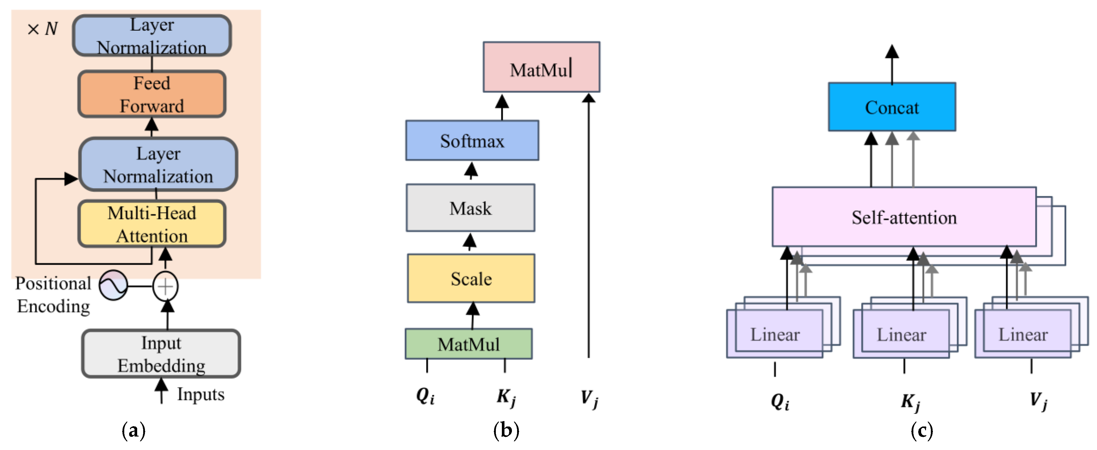
In image classification, the vision transformer (ViT) is widely used, with its core component being the transformer encoder. The encoder structure consists of two layer-normalization operations and a multi-head self-attention mechanism, as shown in Figure 2a.
N represents the depth of the transformer. As the core mechanism of the transformer, self-attention is responsible for learning global features. The input embeddings are transformed into queries ( Q i ), keys ( K j ), and values ( V j ) through a linear layer. The process involves dot product multiplication and Q i and K j scaling, followed by the computation of the autocorrelation coefficient using the softmax function. This coefficient is then multiplied by V j to generate the final self-attention matrix. The process is illustrated in Figure 2b, with the corresponding following mathematical expression:
A ¯ = s o f t m a x Q i T K j d k V j
Queries ( Q i ), keys ( K j ), and values ( V j ) represent different components of the self-attention mechanism, while d k denotes the dimensionality of Q i and K j . Multi-head self-attention is illustrated in Figure 2c, with its mathematical formulation given as follows:
M = c o n c a t   ( A ¯ 1 ,   A ¯ 2 ,   ,   A ¯ n ) W
M represents multi-head self-attention, n represents the number of self-attention heads, A ¯ i represents the self-attention mechanism, and W is the learnable weight matrix.
Although transformers have demonstrated significant advantages in computer vision, their application is constrained by their high computational cost. The primary objective of lightweight transformers is to reduce this complexity by linearizing the softmax function in the self-attention mechanism. Several approaches have been proposed to achieve this. Rewon et al. [41] introduced a method that integrates both local and atrous self-attention into sparse self-attention, resulting in a linearized softmax function. The authors of [42] replaced the self-attention mechanism with a combination of deep and point-wise convolutions. In addition to using the linear function to approximate softmax, the authors of [43,44] proposed approximating the softmax function using a low-rank matrix or third-order polynomials. However, linear transformer performance in downstream tasks remains suboptimal and the application of lightweight transformers in hyperspectral image (HSI) classification is therefore still limited.

2.3. MambaOut

In image classification, MambaOut has been shown to achieve a similar performance to Mamba. As MambaOut is composed solely of convolutional layers and activation functions, its structure is suitable for microprocessors. Therefore, we adopted it as the spatial feature extraction branch basic architecture in this study.
The standard MambaOut, composed of four stacked gated CNN (GCNN) blocks and three downsampling layers, is shown in Figure 3. Of these layers, the downsampling layers adopt convolution for feature downsampling. The core structure of MambaOut is the GCNN block. If the input is X , the GCNN block can be formulated as follows:
X ^ = N o r m ( X )
X C N N = C o n v X ^ w 1 σ X ^ w 2 w 3
where X ^ represents the intermediate variable; X C N N represents the gated CNN block output variable; Norm(·) represents normalization; w 1 , w 2 , w 3 are weights, a learnable parameter with linear operation; and σ is the Gelu activation function.
However, multi-scale global feature extraction cannot be achieved with only one convolution layer; more of these would produce more parameters. In order to improve the lightweight model’s expression ability, we propose the lightweight multi-head MambaOut with a CosTaylorFormer in order to achieve a lightweight module and better classification accuracy.

3. Methods

The framework of the proposed network can be seen in Figure 4. It consists of four main components: The first part involves spatial feature extraction. Hyperspectral images (HSIs) contain both spatial and spectral information, and incorporating spatial features can significantly enhance classification accuracy. To achieve this, spatial features are extracted progressively, moving from local to global. Local spectral features are extracted using the 3D-2D CNN network, a lightweight multi-head MambaOut (LMHMambaOut), with LS2CM as the core module for spatial multi-scale global feature extraction. The second part focuses on spectral feature extraction. Spatial–spectral features are extracted using the 3D-2D CNN network; then, they are focused in the spectrum using an average pooling squeeze feature. The CosTaylorFormer architecture is introduced to capture global spectral features. The third part involves the dynamic information fusion strategy, which fuses the spatial and spectral features. The fourth part uses an MLP layer for classification.

3.1. Spatial Feature Extraction Module

3.1.1. Local Spatial Feature Extraction

Hyperspectral 3D data can be represented as X ϵ R H × W × C , where the spatial dimensions α , β are the core elements used to create 3D patches and spectral dimensionality is reduced through principal component analysis (PCA). Finally, the input features of HSIs can be expressed as X ϵ R p × p × B , where p denotes the patch size and B denotes the spectral dimensionality. For spatial information extraction, a multi-scale 3D-2D network is employed to extract local spatial features. The extracted features are then processed through two 3D convolutional layers with kernel sizes of 1 × 3 × 3 and 1 × 5 × 5. The 3D convolution process is as follows:
X i ,   j x y z = f b i ,   j + m p = 0 p i 1 q = 0 q i 1 t = 0 T i 1 W i ,   j ,   m p ,   q ,   t · X i 1 ,   j x + p y + q z + t
where p, q , and t represent the length, width, and number of spectral bands of the convolution kernel, respectively. W i , j , m p , q , t denotes the weight connected to the mth feature of the i 1 th layer and f represents the activation function.
After two 3D convolutions, spatial information is transformed from a 2D to 1D vector. The hyperspectral data are then expressed as X ϵ R N × C , where N = H × W . These features are subsequently processed using a 2D convolution with a kernel size of 3 × 3. The 2D convolution process is as follows:
X i ,   j x y = f b i ,   j + m p = 0 p i 1 q = 0 q i 1 W i ,   j ,   m p ,   q · X i 1 ,   m x + p y + q
where m is the number of features in layer i 1 ; p i and q i are the length and width of the convolution kernel; W i , j , m p , q is the weight associated with the connection between the kernel position ( p , q ) and the m th feature map in layer i 1 ; b i , j represents the bias of the j th feature in layer i ; and X i 1 ,   m x + p y + q is the eigenvalue of the m th feature map in layer i 1 at position x + p y + q .
After extracting local spatial information, global spatial features were extracted using the LMHMambaOut module. To ensure a lightweight network, the LS2CM was used instead of standard convolution in LMHMambaOut. Residual connections were incorporated to mitigate the risk of gradient vanishing. The spatial feature extraction module consists of two 3D convolutional layers, one 2D convolution layer for spatial local feature extraction, and LMHMambaOut for global spatial extraction. The specific structure spatial feature extraction module is shown in Table 1.

3.1.2. LMHMambaOut

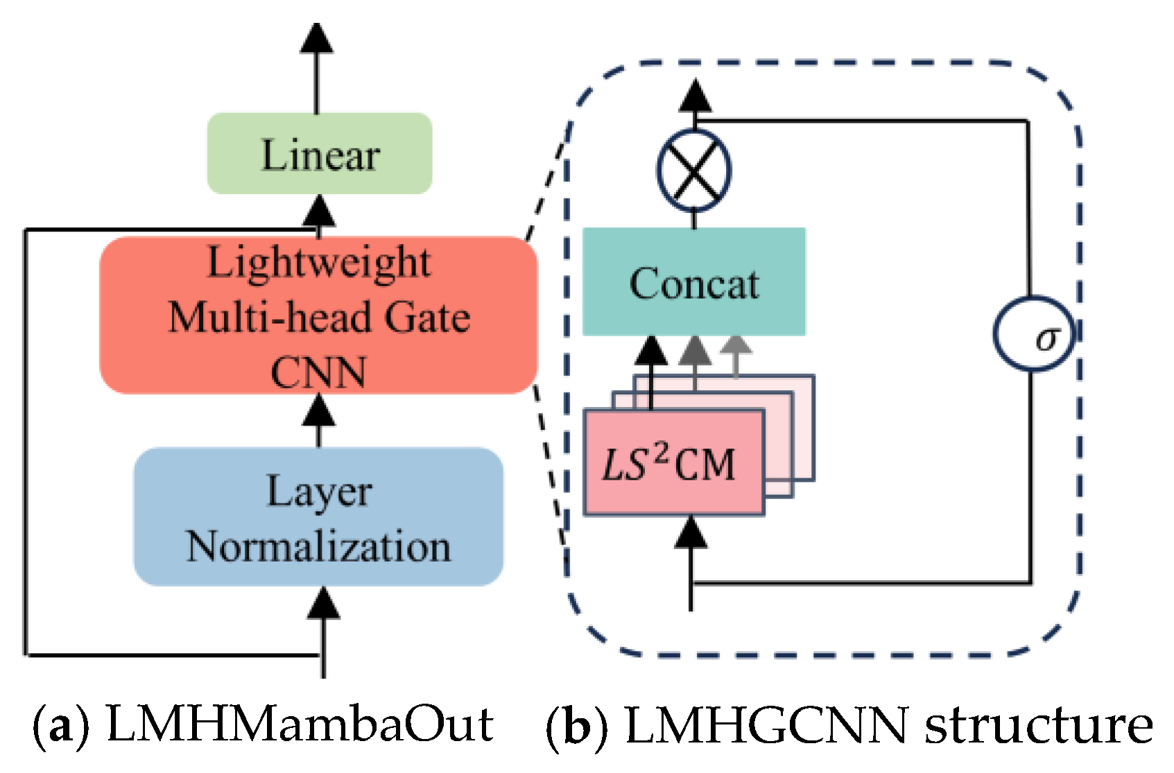
The process of LMHMambaOut consists of a lightweight multi-head gate CNN(LMHGCNN), layer normalization, and a linear layer. It adopts residual connection, as shown in Figure 5a, and the specific process can be described as follows:
X ^ = L i n e a r ( X )
X = L M H G C N N ( L N X i ,   j x y ) + X i ,   j x y
where X i ,   j x y denotes the input feature vector and LN denotes layer normalization. Linear represents the linear layer, and LMHGCNN represents the LMHGCNN operation.
Since it is necessary to extract the global spatial information from multiple scales, we optimized the gate CNN block of the MambaOut core module and proposed a lightweight multi-head gate CNN(LMHGCNN), as shown in Figure 5b.
LMHGCNN is the LMHMambaOut core module. Compared with the core module (GCNN) of MambaOut, standard convolution was substituted with LS2CM. To make up for the fact that GCNN cannot extract global features at multiple scales, LMHGCN adopts LS2CM parallel connections of different convolutional kernels to establish multi-scale global context relationships quickly and effectively. The LMHGCNN can be described as follows:
L M H G C N N = X t o k e n σ ( X L N )
where X t o k e n represents the features after multi-scale fusion vector, σ denotes the Gelu activation function, and X L N denotes the output of the input X i ,   j x y after passing through layer normalization. The activation function represents the activation spatial features and assigns different weights to different spatial feature positions to represent spatial context dependency. The multi-scale LS2CM is used to activate the rich spectral semantic information, which is expressed as follows:
X t o k e n = c o n c a t ( L S 2 C M 1 ,   L S 2 C M 2 ,   L S 2 C M 3 )
where L S 2 C M 1 , L S 2 C M 2 , and L S 2 C M 3 represent depth-wise convolution kernel sizes of 1 × 1 , 3 × 3 , and 5 × 5 , respectively.

3.2. Spectral Feature Extraction Module

3.2.1. Local Spectral Information Extraction

Spectral information extraction consists of two steps: extracting local spectral information using a 3D-2D network and extracting the global equivalent with cosTaylorFormer. To comprehensively capture local spectral features, two 3D convolutional layers with kernel sizes of 3 × 1 × 1 and 5 × 1 × 1 were employed for multi-scale feature extraction in the spectral dimension. After converting spatial information into a 1D representation, a 2D convolution with a kernel size of 3 × 3 was applied to integrate spatial–spectral features. Finally, a global average pooling operation was performed to reduce spatial data variance, emphasizing spectral information as the primary focus. The average pooling operation for information X in the ith channel is defined as follows:
X i = 1 H × W i =   1 H j =   1 W X i ,   j

3.2.2. CosTaylorFormer

We linearized the transformer based on the characteristics of HSI with the aim of reducing its quadratic time and computational complexity. The root cause of the quadratic complexity originates from the self-attention mechanism. To address this, we proposed CosTaylorFormer, which incorporates CosTaylor self-attention as its central mechanism. Inspired by the authors of [45], we introduced the cosine function into TaylorFormer. The specific CosTaylor self-attention design process is as follows:
A ¯ = i e x p Q i T K j / d V j T j = 1 N e x p Q i T K j / d
where A ¯ denotes the self-attention mechanism. Q i R h w × D , K j R h w × D , and V j R h w × D . e x p denote the softmax function, which is an exponential function with a quadratic, thus linearized. When the exponential function is expanded using the Taylor series, the self-attention mechanism can be described as follows:
A t a y l o r = j = 1 N 1 + Q i T K j + 1 2 ! ( Q i T K j ) 2 + 1 3 ! ( Q i T K j ) 3 + + 1 N ! ( Q i T K j ) N V j T j = 1 N 1 + Q i T K j + 1 2 ! ( Q i T K j ) 2 + 1 3 ! ( Q i T K j ) 3 + + 1 N ! ( Q i T K j ) N = j = 1 N 1 + Q i T K j + ο Q i T K j V j T j = 1 N 1 + Q i T K j + ο Q i T K j
where A t a y l o r represents the self-attention mechanism of Taylor series expansion. Linearizing the self-attention mechanism, the higher-order terms tend to approach zero. Ignoring the minimum term and leave only the linear term, the Taylor self-attention mechanism can be described as follows:
A t a y l o r = j = 1 N 1 + Q i T K j V j T j = 1 N 1 + Q i T K j
where A t a y l o r represents the Taylor self-attention mechanism. The exponential function is expanded using a first-order Taylor series. After neglecting the higher-order terms, the original non-linearity is approximated by a linear function, which inevitably introduces an approximation error. Unlike the authors of [41], who employed multi-scale feature extraction, we adjusted the weights based on the spectral curve characteristics of hyperspectral features to enhance training stability. The IP dataset serves as an example here. We randomly selected the more common spectral curves in agricultural classification, chose corn-no-till as the representative of crops, and selected grass-tree and wood as the representatives of common green plants, with the spectral curve characteristics of the wood, grass-tree, and corn-no-till classes extracted, as shown in Figure 6a.
By comparing the spectral curve in Figure 6a, it was found that the spectral curve is approximately the Gaussian function curve. Taking the spectral curve of trees as an example, it was compared with the Gaussian function. When comparing the extracted spectral curve of wood data with the Gaussian function, it generally aligns with a Gaussian normal distribution, as illustrated in Figure 6b. However, weight readjustment primarily considers two factors: (1) the degree to which data conform to the distribution characteristics of the spectral curve, along with its physical interpretability, and (2) the introduction of a decomposable function to induce deviation in the attention matrix. Based on these considerations, we proposed CosTaylorFormer, which incorporates the cosine function for weight readjustment.
This approach offers two advantages. First is that the half-cosine waveform closely resembles the Gaussian waveform. The mathematical expression of the Gaussian function is as follows:
f x = e x 2 2 σ 2
In the formula, x represents any numerical value, σ 2 represents the variance, indicating that the peak value is 1 when x = 0 .
The mathematical expression of the half-cosine function is as follows:
g x = 1 2 ( 1 + c o s π x β , x β   0   ,   x β  
β is a non-zero interval. The half-cosine is consistent with the Gaussian function, and its peak value is 1 when x = 0 .
To compare the similarity between the Gaussian function and the half-cosine, we let β = π σ in the half-wave cosine, indicating that their widths are consistent. The Taylor series expansion at x = 0 , ignoring the higher-order terms; those of the Gaussian function and the half-cosine are, respectively, shown in Formulas (15) and (16):
e x 2 2 σ 2 1 x 2 2 σ 2 + x 4 8 σ 4
1 2 ( 1 + c o s x σ = 1 x 2 4 σ 2 + x 4 48 σ 4  
The second-order terms of both functions are negative quadratic terms, and the second-order approximation error is x 2 4 σ 2 . We calculate the mean square error (MSE) for the Gaussian and half-cosine functions within the interval a , a . The MSE can be described as follows:
M S E = 1 2 a a a ( e x 2 2 σ 2 1 2 ( 1 + c o s π x β ) 2 d x
We let β = 1 , a = 1.5 , and M S E 0.0027 . That is to say, the smaller the width of the half-cosine function, the closer it is to the Gaussian function. The MSE is within 0.005 within the approximate range of [−2, 2]. Image analysis is conducted on two functions with an amplitude of 1 within the range of [−4, 4], analyzing the graph shown in Figure 6c. It can be seen that, within the range of [−1, 1], the two functions basically overlap. The purpose of using the half-cosine function for weight adjustment is to assign high weight values to positions close to the center of the pixel and low values to those that are far away so as to infer the long-distance dependency. Therefore, the half-cosine function is effective.
The second advantage of adopting the cosine function is as follows. Cosine weights can be decomposed into the summation of two functions; this does not increase the complexity of the model, but is beneficial in facilitating linearization.
We add the cosine function to Q i T K j in A t a y l o r for weight adjustment, the mathematical description of which is as follows:
Q i T K j = Q i T K j c o s π i j 2
According to the formula for the sum of two cosine function angles, the above can be described as follows:
Q i T K j cos π i j 2 = Q i T K j c o s π i 2 c o s π j 2 + s i n π i 2 s i n π j 2 = Q i T c o s π i 2 K j c o s π j 2 + Q i T s i n π i 2 K j s i n π j 2 = Q i c o s π i 2 T K j c o s π j 2 + Q i s i n π i 2 T K j s i n π j 2
where Q i ,   K j ϵ R N × d , i ,   j = 1 ,   N , N = h × w represent the space size of the input patch. We let Q i c o s = Q i c o s π i 2 , Q i s i n = Q i s i n π i 2 , K j c o s = K j c o s π j 2 , K j s i n = K j s i n π j 2 . According to the associative law for matrix multiplication, the CosTaylor self-attention mechanism in CosTaylorFormer can be described as follows:
A = j = 1 N 1 + Q i c o s T K j c o s + Q i s i n T K j s i n V j T j = 1 N 1 + Q i c o s T K j c o s + Q i s i n T K j s i n = j = 1 N V j T + Q i c o s T K j c o s V j T + Q i s i n T K j s i n V j T j = 1 N 1 + Q i c o s T K j c o s + Q i s i n T K j s i n = j = 1 N V j T + Q i c o s T j = 1 N K j c o s V j T + Q i s i n T j = 1 N K j s i n V j T N + Q i c o s T j = 1 N K j c o s + Q i s i n T j = 1 N K j s i n
The multi-head CosTaylor self-attention mechanism functions similarly to the transformer, aiming to capture multiple features. The process is as follows:
M = c o n c a t ( A 1 ,   A 2 ,   ,   A N ) W
W is the learnable weight, A i is self-attention at different scales.
According to the comparison of computational complexity, the self-attention mechanism has a complexity of   O ( 2 N 2 d ) . Given that N 2 d in the experimental setting, the complexity of the self-attention mechanism is approximately O ( N 2 ) . In contrast, the complexity of the CosTaylor self-attention mechanism is O ( 2 d 2 N ) O ( N ) . Therefore, its linearization enables global feature extraction while significantly reducing both time and space complexity.

3.3. Dynamic Information Fusion Strategy

Hyperspectral images contain rich spectral information, and classification accuracy can be improved by incorporating spatial information. However, simply applying the Add or Concat operations to spatial and spectral information leads to redundancy. To address this, we propose a dynamic information fusion strategy. As illustrated in Figure 4, this strategy consists of three key processes: information stacking, gate control, and dynamic feature fusion.
Spatial features are denoted as X s p a ϵ R N × C , while spectral features are represented as X s p c ϵ R N × C . The objective is to concatenate spatial and spectral information while regulating their flow through gate control. Concatenation of spatial and spectral features is performed as follows:
X ~ = s t a c k X s p a ,   X s p c
The concatenated features are represented as X ~ ϵ R N × C × Z , where Z denotes the two dimensions (spatial and spectral) in the concatenated space. The gate control process regulates the spatial and spectral feature information flows, primarily through soft attention. Specifically, the feature information X ~ ϵ R N × C × Z along dimension Z is extracted and processed using the softmax function:
a = e A X ~ e A X ~ + e B X ~ ,   b = e B X ~ e A X ~ + e B X ~
where a and b are the vectors generated by the soft attention mechanism, where A   ϵ R 1 × Z and B   ϵ R 1 × Z , w i t h   a and b satisfying the condition a + b = 1 . a and b act as weight coefficients for the spatial and spectral information flows, respectively. The final output feature, represented as X ~ o u t ϵ R N × C , is expressed as follows:
X ~ o u t = a · X s p a + b · X s p c ,   a + b = 1  

4. Results

In this section, we first introduce the experimental data and then provide a detailed explanation of the experimental settings. The effectiveness of the proposed network is demonstrated through comparisons with several popular models.

4.1. Data Description

Experiments were conducted using four publicly available hyperspectral datasets from four different countries: India, Italy, the United States, and China. The dataset categories and sample numbers are shown in Table 2, and the specific details are as follows:
IP: The Indian Pines dataset was gathered by an airborne visible infrared imaging spectrometer (AVIRIS) over northwestern Indiana, USA. The data consist of 145 × 145 pixels and 224 spectral reflection bands; the spatial resolution is approximately 20 m. This dataset includes agriculture-related classes (about two-thirds of the data) as well as forest and natural perennial plants (about one-third). In addition to vegetation, the scene also contains two-lane highways, a railway line, houses, low-density buildings, and smaller roads. The coverage rate of non-vegetation classes is less than 5%, as crops such as corn and soybeans were in their growing season.
WHU-Hi-LongKou: Data were obtained by the headwall nano-hyperspec sensor on the unmanned aerial vehicle (UAV) platform in Longkou Town, Hubei Province, China. The dataset consists of 550 × 400 pixels and 270 spectral reflection bands, and the spatial resolution of the UAV-borne hyperspectral imagery is about 0.463 m. WHU-Hi-LongKou preprocessing includes radiation calibration and geometric correction. The major categories included urban asphalt surfaces, bricks, and metal sheets.
SA: Data were gathered by AVIRIS over the Salinas in northern California. The dataset consists of 512 × 217 pixels and 224 spectral reflection bands; the spatial resolution is 3.7 m. The classification primarily focused on identifying fruits and cultivated land.
PU: Data were collected by a reflective optics system imaging spectrometer (ROSIS) over Pavia University in northern Italy. The dataset consists of 610 × 610 pixels and 103 spectral reflection bands; the spatial resolution is 1.2 m. The PU dataset contains a total of nine land feature categories.

4.2. Experimental Settings

Experiments were conducted on an Intel Xeon (R) Gold 6226R processor and an NVIDIA RTX 4000 graphics processing unit (GPU), both equipped with 8 GB of RAM. The program was implemented using the PyTorch 2.0.0 architecture in Python (3.9.13). To evaluate the performance of the proposed network, classification accuracy was assessed using the following evaluation metrics: overall accuracy (OA), average accuracy (AA), and Kappa statistic. Network complexity was evaluated based on the number of parameters and floating-point operations (FLOPs). The number of parameters represents the video memory occupied, while FLOPs indicate the computational capability required from the GPU. Training and test times were also assessed as auxiliary metrics.
The spatial window size for our network was set to 21 × 21. Due to the high spectral band overlap, PCA was used for spectral band selection, the value of which was set to 30. In CosTaylorFormer, the depth was set to 1, and the number of heads in the multi-head CosTaylor self-attention mechanism was set to 2. The proposed network epoch was set to 150, with a learning rate of 0.001. The Adam optimizer was used for training. For comparative networks, parameter settings followed the optimal values from the original article.
All experiments were conducted using four public datasets: IP, WHU-Hi-Longkou, SA, and PU. For the IP dataset, 10% of each data category was randomly selected for training, while the remaining data served as the test set. Similarly, for the other three datasets (WHU-Hi-Longkou, SA, and PU), 1% of each data category was randomly selected for training, and the rest was used as the test set.

4.3. Classification Results

To evaluate the accuracy and complexity of the proposed network, we compared it with nine classic networks: the traditional SVM [6], 2D CNN [9], HybridSN [23], deep pyramidal residual network (DpresNet) [18] (based on the CNN network), ViT [24], CTMixer [26] (based on the transformer network), and several lightweight networks including ResNet-LS2CM [40], lightweight spectral–spatial squeeze-and-excitation residual bag-of-features learning network (S3EresBof) [46], and LSGA-VIT [33]. All experimental results are reported as the mean and variance of ten runs. Table 3, Table 4, Table 5 and Table 6 present a quantitative comparison of the classification accuracy of the proposed network with the nine other networks across four datasets (i.e., IP, WHU-Hi-Longkou, SA, and PU).
(1) Classification accuracy analysis. The classification results show that the traditional SVM algorithm achieves the lowest accuracy, significantly underperforming compared to deep learning methods. As can be seen in Table 3, on the IP dataset, our method outperforms ViT with an OA improvement of 1.84%, an AA increase of 4.26%, and a Kappa score of 2.15% higher. Compared to the CTMixer network, which combines ViT with a CNN backbone, our network achieves a 0.15% higher OA, a 0.12% higher AA, and an almost identical Kappa score. Additionally, when compared to the deep CNN-based DPresNet, our network achieves a 0.81% higher OA, a 0.95% higher AA, and a 0.93% higher Kappa score.
From the analysis of the classification accuracy of each category, there are a total of 16 categories of IP dataset. The network we proposed has achieved the best classification accuracy in 12 categories. Among them, the classification accuracy of eight categories reached 100%.
Similar classification results were obtained for the other datasets. The proposed network slightly outperformed CTMixer in terms of classification accuracy, primarily because both networks account for global and local features in their structures. The advantage of our network lies in its incorporation of spectral features, as well as its ability to enhance the transformer based on spectral Gaussian normal distribution characteristics. Additionally, since excessive spectral information can lead to overlap, we applied the PCA method to extract the main spectral features. In contrast, the CTMixer network inputs all the spectral information into the network, which may cause information overlap and negatively impact classification accuracy. However, the accuracy of the proposed network did not show significant improvement compared to the CTMixer network, primarily due to the number of model parameters.
From the analysis of the classification accuracy of each category, among the other three datasets, more than 50% of the categories have reached the optimal classification accuracy.
(2) Complexity and classification accuracy comprehensive evaluation. Since the hyperparameter settings of the model are consistent, the number of model parameters remains fixed. Due to the small number of training samples in IP dataset and the imbalance in the number of samples within classes, the classification performance of different networks can be significantly compared on the IP dataset. The IP dataset is used as an example here.
Table 7 compares model complexity using a number of parameters. The number of parameters represents the number of parameters of a model, which is expressed in units of M as 10 6 and FLOPs as primary metrics, FLOPs represents the number of floating-point operations per second, with G as the unit as 10 9 , with model training and testing time as secondary metrics. The training time refers to the period from the start of model training to the preservation of the best model, and it is measured by S-time. The test time is the period from when the test data enter the model to when the classification results are output, and it is timed in seconds.
The classification accuracies of the proposed network and CTMixer are approximately the same. Therefore, we first compared their complexities. In this regard, the parameter count and FLOPs of our network are only 33% and 14% those of CTMixer. Compared to LGSA-VIT, which shows the highest accuracy among lightweight modules, the parameter count of the proposed network was reduced by approximately 57%. Overall, our network has more parameters than the LS2CM network alone, but OA was higher by about 4% and AA was 14% higher. However, the testing time of our network model is the shortest among all networks, indicating that the proposed model is more lightweight when applied to the same test dataset.
However, the proposed network still has limitations. While it meets the requirements for a lightweight network without compromising accuracy, a quantitative analysis of classification accuracy and model complexity shows that it does not substantially outperform other networks in terms of the former. Additionally, the parameter count of the proposed network is not the lowest. However, the network we proposed meets lightweight requirements. In systems with limited resources, lightweight networks require the number of parameters to be less than 1M. The network we proposed achieves the best classification accuracy and strikes a balance between lightweight and performance qualities.
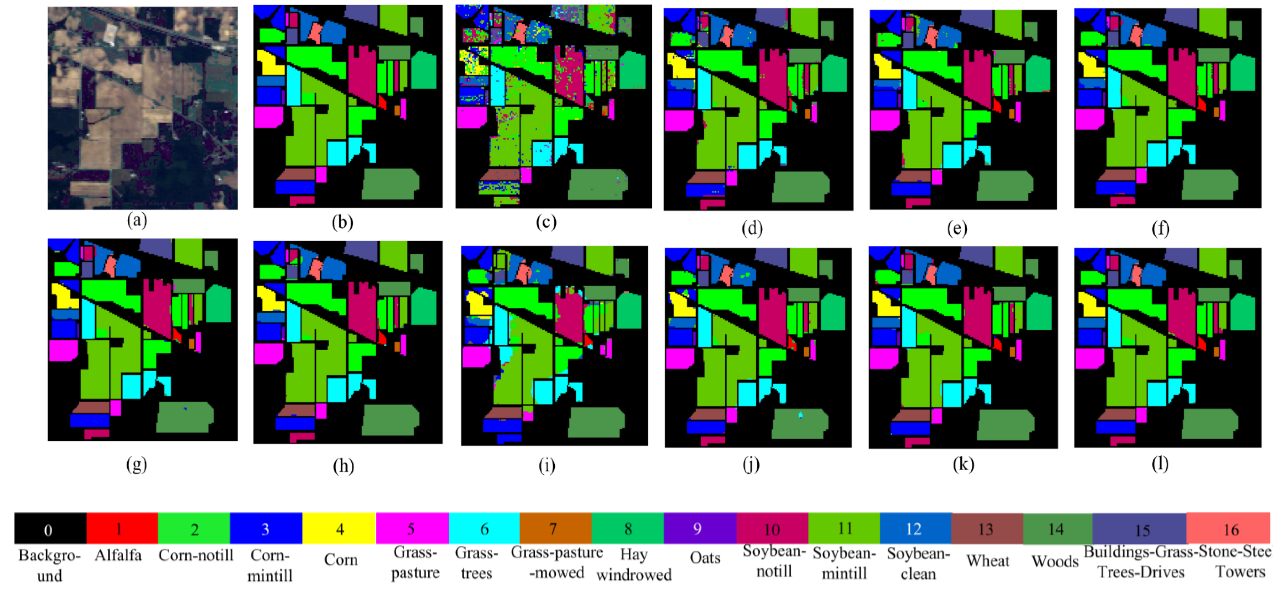
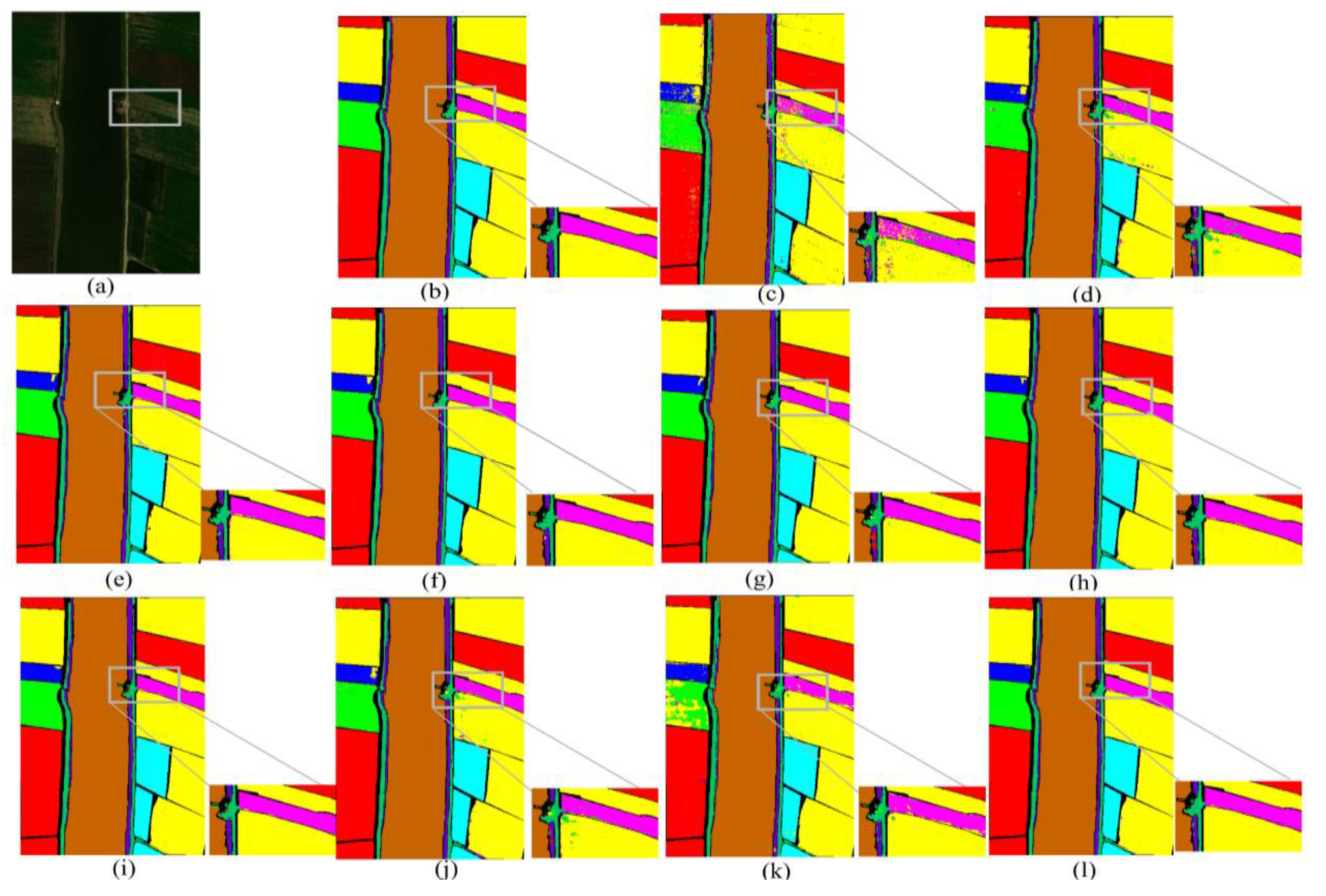
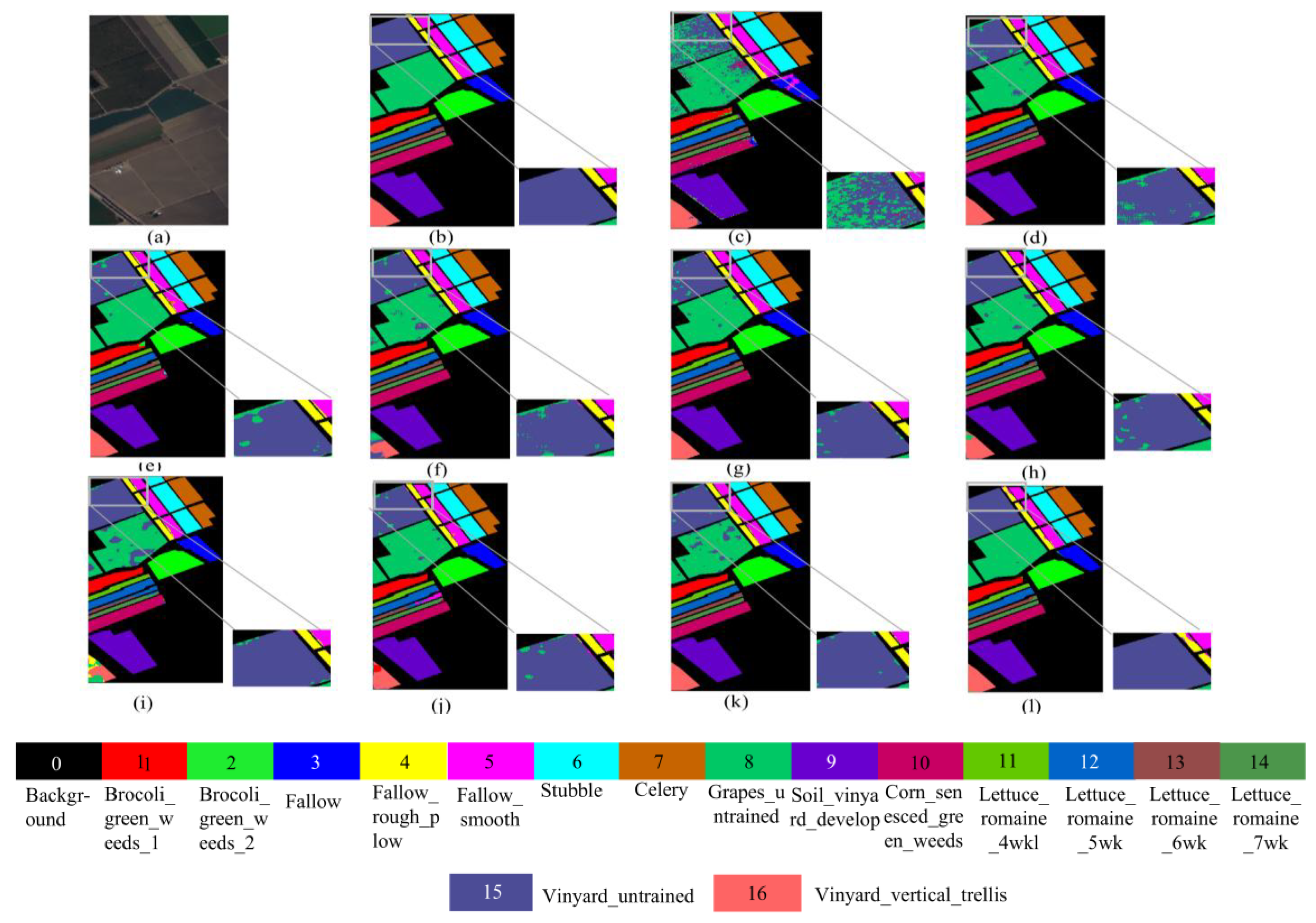
(3) In terms of qualitative analysis, the best trained model was visualized. Figure 7, Figure 8, Figure 9 and Figure 10 display the results on the IP, WHU-Hi-LongKou, SA, and PU datasets. The visualizations for these datasets highlight regions with significant misclassifications, as indicated by the boxes.
On the IP dataset, the area marked with the gray box in the figure is selected for magnification. The main reason is that the area occupied by each category in this area is relatively small. At the same time, the three different types are closely connected, the edge areas are easily confused, and the shape of this area is irregular. The performance of the model can be reflected by observing the classification effect of this area. On the WHU-HI-Longkou dataset, the area of Category 8 is taken as the key comparison area. There are mainly two reasons. Firstly, the training samples for Category 8 are relatively small, making precise discrimination more difficult. Secondly, the distribution of Category 8 is relatively scattered, and the edges of some concentrated areas are irregular, making it difficult to distinguish the boundary areas. On the SA dataset, the key observation area was selected as Area 15 of category, and the edge classification effect of this part was mainly observed. The characteristic of this area is that it is adjacent to Category 8, and the number of training samples in Category 8 is the largest among all categories, which is easily confused with the observation area. On the PU dataset, the main reason for choosing this area as the key observation area is that the irregular edge of this area leads to classification errors in most networks within this area.
The classification results show that our network has fewer errors overall. Specifically, our network exhibits lower classification errors in areas with higher complexity, while misclassifications are minimal in regions with more easily distinguishable samples. Additionally, as can be seen in Figure 10, most networks have many classification error points in this area, and they are mainly distributed in the edge part, resulting in the inability to accurately segment this area, the PU dataset reveals that our proposed network produces smooth, well-defined edges and there are fewer classification error points.
(4) Feature distribution analysis. The IP dataset is characterized by a smaller number of data samples, a larger number of classification types, and more dispersed distributions thereof, making classification more challenging. On the IP dataset, the classification accuracy of different networks varies significantly; the better the network performance, the higher the classification accuracy. To illustrate this, we used the 2D t-SNE method to extract features from the classification results of various networks, as shown in Figure 11. Figure 11a shows the original feature distribution. Different colors represent different categories of features. The spatial spectral features at different positions in the image are different, so the initial feature distribution is completely random. The coordinates in the figure represent the relative positions of different features. Initially, features of different categories overlap each other with relatively small intervals, and features of the same category are scattered. After feature extraction, most networks can aggregate the features of the same category well together, but there are still many scattered feature points distributed in other categories. From the perspective of the coordinate axes, different features are still distributed relatively compactly, such as Figure 11b 2D CNN, (d) DPResNet, and (h) S3EresBof. Especially the 2D CNN, which exhibited the poorest classification performance, shows more incorrectly positioned features and a scattered arrangement of similar features. The proposed network performs better at aggregating similar features; there are hardly any scattered feature points distributed in other category areas. It is indicated that the proposed network can better distinguish different categories and better aggregate the features of the same category together.

5. Discussion

5.1. Ablation Experiment

(1) To validate the effectiveness of the network, we took the 3D-2D network extracted from shallow local spatial–spectral features as the baseline before adding the LMHMambaOut, CosTaylorFormer and dynamic information fusion modules. To assess the effectiveness of the dynamic information fusion strategy (DIFS), the information fusion part adopts the add operation.
The classification results are shown in Table 8. The classification accuracy was lowest when only baseline and few FLOPs were used. This indicates that the computational complexity is relatively low when only using the 3D-2D network model. However, combining LMHMambaOut and CosTaylorFormer features resulted in improved classification accuracy. However, when LMHMambaOut was added, the FLOPs increased significantly, because LMHMambaOut is composed of convolution. The number of model parameters is generated during the feature extraction process. Meanwhile, during the final classification, the two-dimensional feature vectors of the spatial spectrum need to be converted into one-dimensional equivalents, and linear layer classification is adopted. At this time, the number of parameters increases significantly. The computational complexity also increases accordingly. When CosTaylorFormer was added, the number of model parameters actually decreased. This is because CosTaylorFormer performs pooling operations on the input sequence, effectively reducing the number of parameters. Meanwhile, CosTaylorFormer is independent of the length of the input sequence and only related to the embedded feature dimension, which is much smaller than the length. Therefore, introducing CosTaylorFormer significantly reduces the number of model parameters. However, due to the matrix operations inside CosTaylorFormer, the FLOPs increase slightly. Additionally, the adoption of DIFS effectively enhanced the classification accuracy; OA increased by approximately 1% at most, and 0.3% at least, with a negligible impact on the number of model parameters and FLOPs.
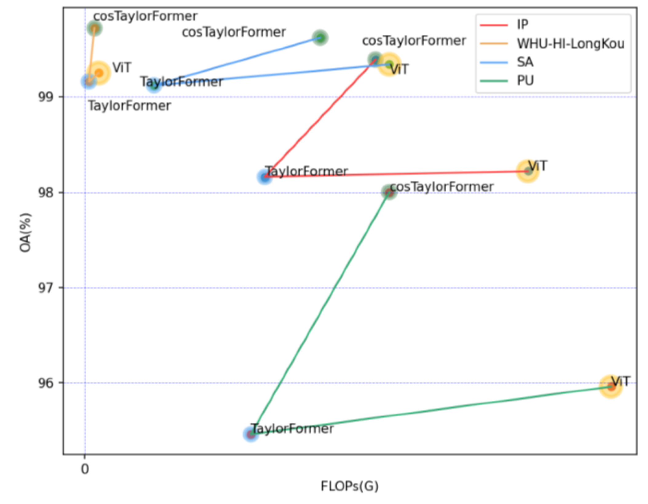
(2) Verification of CosTaylorFormer. To assess the effect of CosTaylorFormer, we focused solely on the spectral branch. In this experiment, the CosTaylorFormer structure was replaced by ViT and TaylorFormer. Since the performance of these three models is affected by the number of heads in the self-attention mechanism and the depth of the model, generally speaking, the more heads there are and the deeper the depth, the better the model performance. To ensure a fair comparison and eliminate any influence from the depth and head number of CosTaylorFormer, and thus demonstrate its stronger expressiveness, we set both the depth and head number to one for ViT, TaylorFormer, and CosTaylorFormer, instead of using their optimal values.
Figure 12 shows the OA, FLOPs, and parameter quantities of different models on four datasets. In the figure, the horizontal and vertical coordinates represent FLOPs and OA, and the size of the circle represents the number of parameters. Under the same hyperparameter settings (depth: 1, head: 1), TaylorFormer exhibits the lowest classification accuracy, despite its linear structure, under the same depth and head number. On the IP dataset, TaylorFormer not only has the lowest overall accuracy (OA) but also the smallest number of parameters and FLOPs. This comparison with ViT confirms the effectiveness of the CosTaylorFormer structure. The OA of CosTaylorFormer is higher than that of TaylorFormer, and classification accuracy increased significantly across all other datasets. Moreover, the circle size of CosTaylorFormer is almost the same as that of TaylorFormer, indicating that the number of parameters of the two models is almost the same, but much smaller than that of ViT, demonstrating that CosTaylorFormer achieves the best classification performance while using fewer parameters than ViT.
(3) To validate the dynamic information fusion strategy, we applied the optimal parameter settings (depth: 1, head number: 2) to CosTaylorFormer. We performed Add and Concat operations on the spatial and spectral features and compared the results with those of the proposed dynamic information fusion strategy. The outcomes across four datasets are shown in Table 9. On the IP dataset, the dynamic information fusion strategy improved the OA by 0.45%, the AA by 1.47%, and the Kappa coefficient by 0.51% compared to the direct Add operation. It also improved the OA by 0.36%, the AA by 0.49%, and the Kappa by 0.42% over the Concat operation. Similar results were observed on the other datasets. These findings confirm that the dynamic information fusion strategy enhances classification accuracy across all datasets.

5.2. Hyperparameter Setting

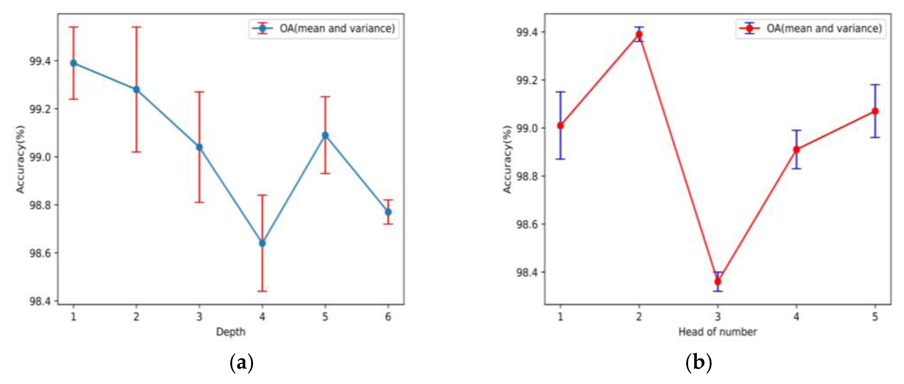
(1) The depth and head number of CosTaylorFormer. Classification accuracy is influenced by the depth and number of multi-head self-attention layers in CosTaylorFormer. To determine the optimal parameters, we conducted ten experimental runs using overall accuracy (OA) as the benchmark; the variance is represented in the form of error bars. The depth was varied from one to six, while the number of heads ranged from one to five. Since the general depth and the number of heads are manually set as integers, the OA values between different depths or the number of heads are presented in a linear connection manner. Taking the IP dataset as an example, as shown in Figure 13, it is clear that the optimal configuration for CosTaylorFormer is a depth of one and two heads.
(2) Patch size and number of spectral bands. The selection of patch size and the number of spectral bands significantly influences the accuracy of hyperspectral image (HSI) classification. The hyperspectral input is represented as X ϵ R B × w × w , where w denotes the patch size and B represents the number of selected bands. Increasing w allows for more spatial information to be incorporated, while increasing B enables the inclusion of additional spectral bands. Although incorporating more information can enhance classification accuracy to some extent, excessive spatial information may lead to interference, and redundant spectral information can result in decreased accuracy.
Therefore, an optimal balance between these factors must be established. To investigate this, we conducted experiments using four public datasets with different combinations of patch sizes, w   = 17 , 19 , 21 , 23 , 25 , and spectral band numbers, B   = 20 , 25 , 30 , 35 , drawing the three-dimensional hot spot map and selecting the best parameters of OA. Figure 14 illustrates the OA achieved by each combination. Our findings indicate that the highest accuracy is achieved when w is set to 21 and B to 30.

5.3. Training with Small Samples

To demonstrate that the proposed network is suitable for small-sample datasets, we randomly selected 1% to 5% of the labeled data from the IP dataset and 0.2%, 0.4%, 0.6%, 0.8%, and 1% of those from the WHU-Hi-LongKou, SA, and PU datasets as the training data, with the remaining data used as the test set. Since overall accuracy (OA) yielded the highest values among the accuracy metrics (OA, AA, and Kappa statistic), it was chosen as the evaluation metric for this experiment. As shown in Figure 15, our proposed lightweight network achieved the best classification results when trained with small-sample data, particularly on the SA dataset.

6. Conclusions

For spatial global extraction, we proposed lightweight multi-head MambaOut, which can effectively extract multi-scale spatial features and ensure a lightweight model. Because it only uses convolution, it can be deployed more easily than Mamba in resource-limited systems. The CosTaylorFormer structure proposed in this paper effectively enhanced the classification accuracy of hyperspectral images (HSIs) for spectral features. The linearization of the transformer addressed the quadratic problem, improving its performance. For spatial–spectral information fusion, a dynamic information fusion strategy was introduced to efficiently control information flow according to input feature. Compared to the lightweight network with the highest accuracy, the proposed LMHMambaOut-CosTaylorFormer significantly reduced the number of parameters and FLOPs without sacrificing classification accuracy. More specifically, the number of parameters was reduced by approximately 57% compared to LSGA-VIT. Although the proposed network achieved the highest classification accuracy among lightweight networks, it does not have the fewest parameters. Meanwhile, this lightweight model is proposed mainly for construction in airborne or unmanned aerial vehicle (UAV) on-board systems in the civilian field; therefore, this model is mainly applicable to airborne and UAV on-board hyperspectral data. In the future, we aim to further optimize the network to maintain classification accuracy in leading networks while minimizing complexity.

Author Contributions

Conceptualization, Y.L. and Y.Z.; methodology, Y.L.; validation, Y.L. and Y.Z.; formal analysis, J.Z.; writing—original draft preparation, Y.L.; writing—review and editing, Y.L. and Y.Z.; visualization, Y.L. All authors have read and agreed to the published version of the manuscript. Please consult CRediT taxonomy for explanations of terms.

Funding

This research received no external funding.

Data Availability Statement

Data availability statements are available at https://www.ehu.eus/ccwintco/index.php/Hyperspectral_Remote_Sensing_Scenes and https://rsidea.whu.edu.cn/resource_WHUHi_sharing.htm (last accessed on 13 February 2025).

Acknowledgments

The authors gratefully acknowledge the Group de Inteligencia Computacional and Wuhan University for the publicly available HSI data.

Conflicts of Interest

The authors declare no conflicts of interest.

Abbreviations

The abbreviations for all key terms in this paper are explained below:
HSIHyperspectral Image
SVMSupport Vector Machine
CNNConvolutional Neural Network
LMHMambaOutLightweight Multi-Head MambaOut
ViTVision Transformer
LS2CMLightweight Spectral–Spatial Convolution Module
GCNNGated CNN
LMHGCNNLightweight Multi-Head Gate CNN
MSEMean Square Error
HybirdSNHybird Spectral-Spatial Network
DPresNetDeep Pyramidal Residual Network
CTMixerConvolution Transformer Mixer network
ResNet-LS2CMLightweight Spectral–Spatial Residual Network
S3EresBofLightweight Spectral-Spatial Squeeze-and-Excitation Residual Bag-of-Features Learning Network
LSGA-VITLight Self-Gaussian-Attention Vision Transformer Network
IPIndian Pines
SASalinas
PUPavia University
OAOverall Accuracy
AAAverage Accuracy
KappaKappa Coefficient
FLOPsFloating-Point Operations

References

  1. Moharram, M.; Divya, M. Land Use and Land Cover Classification with Hyperspectral Data: A Comprehensive Review of Methods, Challenges and Future Directions. Neurocomputing 2023, 536, 90–113. [Google Scholar] [CrossRef]
  2. Yuan, J.; Wang, S.; Wu, C.; Xu, Y. Fine-Grained Classification of Urban Functional Zones and Landscape Pattern Analysis Using Hyperspectral Satellite Imagery: A Case Study of Wuhan. IEEE J. Sel. Top. Appl. Earth Obs. Remote Sens. 2022, 15, 3972–3991. [Google Scholar] [CrossRef]
  3. Calin, M.A.; Calin, A.C.; Nicolae, D.N. Application of airborne and spaceborne hyperspectral imaging techniques for atmospheric research: Past, present, and future. Appl. Spectrosc. Rev. 2021, 56, 289–323. [Google Scholar] [CrossRef]
  4. Zhuo, R.; Guo, Y.; Guo, B. A Hyperspectral Image Classification Method Based on 2-D Compact Variational Mode Decomposition. IEEE Geosci. Remote Sens. Lett. 2023, 20, 1–5. [Google Scholar] [CrossRef]
  5. Ham, J.; Chen, Y.C.; Crawford, M.M.; Ghosh, J. Investigation of the Random Forest Framework for Classification of Hyperspectral Data. IEEE Trans. Geosci. Remote Sens. 2005, 43, 492–501. [Google Scholar] [CrossRef]
  6. Melgani, F.; Bruzzone, L. Classification of Hyperspectral Remote Sensing Images with Support Vector Machines. IEEE Trans. Geosci. Remote Sens. 2004, 42, 1778–1790. [Google Scholar] [CrossRef]
  7. Bai, Y.; Sun, X.; Ji, Y.; Fu, W.; Zhang, J. Two-Stage Multi-Dimensional Convolutional Stacked Autoencoder Network Model for Hyperspectral Images Classification. Multimed. Tools Appl. 2023, 83, 23489–23508. [Google Scholar] [CrossRef]
  8. Subba Reddy, T.; Krishna Reddy, V.V.; Vijaya Kumar Reddy, R.; Kolli, C.S.; Sitharamulu, V.; Chandrababu, M. Shbo-Based U-Net for Image Segmentation and Fshbo-Enabled Dbn for Classification Using Hyperspectral Image. Imaging Sci. J. 2023, 72, 479–498. [Google Scholar] [CrossRef]
  9. Hamouda, M.; Ettabaa, K.S.; Bouhlel, M.S. Smart Feature Extraction and Classification of Hyperspectral Images Based on Convolutional Neural Networks. IET Image Process. 2020, 14, 1999–2005. [Google Scholar] [CrossRef]
  10. Wu, Q.; He, M.; Liu, Z.; Liu, Y. Multi-Scale Spatial-Spectral Residual Attention Network for Hyperspectral Image Classification. Electronics 2024, 13, 262. [Google Scholar] [CrossRef]
  11. Ding, Y.; Zhang, Z.; Zhao, X.; Hong, D.; Yu, C.; Cai, W. Multi-Feature Fusion: Graph Neural Network and Cnn Combining for Hyperspectral Image Classification. Neurocomputing 2022, 501, 246–257. [Google Scholar] [CrossRef]
  12. Gao, Y.; Zhang, M.; Wang, J.; Li, W. Cross-Scale Mixing Attention for Multisource Remote Sensing Data Fusion and Classification. IEEE Trans. Geosci. Remote Sens. 2023, 61, 1–15. [Google Scholar] [CrossRef]
  13. Zhang, M.; Li, W.; Zhao, X.; Liu, H.; Tao, R.; Du, Q. Morphological Transformation and Spatial-Logical Aggregation for Tree Species Classification Using Hyperspectral Imagery. IEEE Trans. Geosci. Remote Sens. 2023, 61, 1–12. [Google Scholar] [CrossRef]
  14. He, K.M.; Zhang, X.; Ren, S.Q.; Sun, J. Deep Residual Learning for Image Recognition. In Proceedings of the 2016 IEEE Conference on Computer Vision and Pattern Recognition (CVPR), Las Vegas, NV, USA, 27–30 June 2016; pp. 770–778. [Google Scholar]
  15. Xia, M.; Yuan, G.; Yang, L.; Xia, K.; Ren, Y.; Shi, Z.; Zhou, H. Few-Shot Hyperspectral Image Classification Based on Convolutional Residuals and SAM Siamese Networks. Electronics 2023, 12, 3415. [Google Scholar] [CrossRef]
  16. Banerjee, A.; Banik, D. Resnet Based Hybrid Convolution Lstm for Hyperspectral Image Classification. Multimed. Tools Appl. 2023, 83, 45059–45070. [Google Scholar] [CrossRef]
  17. Zhang, J.; Zhao, L.; Jiang, H.; Shen, S.; Wang, J.; Zhang, P.; Zhang, W.; Wang, L. Hyperspectral Image Classification Based on Dense Pyramidal Convolution and Multi-Feature Fusion. Remote Sens. 2023, 15, 2990. [Google Scholar] [CrossRef]
  18. Paoletti, M.E.; Haut, J.M.; Fernandez-Beltran, R.; Plaza, J.; Plaza, A.J. Deep Pyramidal Residual Networks for Spectral-Spatial Hyperspectral Image Classification. IEEE Trans. Geosci. Remote Sens. 2019, 57, 740–754. [Google Scholar] [CrossRef]
  19. Ding, C.; Chen, Y.; Li, R.; Wen, D.; Xie, X.; Zhang, L.; Zhang, Y. Integrating Hybrid Pyramid Feature Fusion and Coordinate Attention for Effective Small Sample Hyperspectral Image Classification. Remote Sens. 2022, 14, 2355. [Google Scholar] [CrossRef]
  20. Ma, Q.; Zhang, X.; Zhang, C.; Zhou, H. Hyperspectral Image Classification Based on Capsule Network. Chin. J. Electron. 2022, 31, 146–154. [Google Scholar] [CrossRef]
  21. Cui, Y.; Li, W.; Chen, L.; Gao, S.; Wang, L. Double-Branch Local Context Feature Extraction Network for Hyperspectral Image Classification. IEEE Geosci. Remote Sens. Lett. 2022, 19, 6011005. [Google Scholar] [CrossRef]
  22. Zhang, X.; Guo, Y.; Zhang, X. Hyperspectral Image Classification Based on Optimized Convolutional Neural Networks with 3d Stacked Blocks. Earth Sci. Inform. 2022, 15, 383–395. [Google Scholar] [CrossRef]
  23. Roy, S.K.; Krishna, G.; Dubey, S.R.; Chaudhuri, B.B. Hybridsn: Exploring 3-D–2-D Cnn Feature Hierarchy for Hyperspectral Image Classification. IEEE Geosci. Remote Sens. Lett. 2020, 17, 277–281. [Google Scholar] [CrossRef]
  24. Vaswani, A.; Shazeer, N.; Parmar, N.; Uszkoreit, J.; Jones, L.; Gomez, A.N.; Polosukhin, I. Attention Is All You Need. In Proceedings of the Neural Information Processing Systems (NIPS), Longbeach, CA, USA, 4–9 December 2017. [Google Scholar]
  25. Hong, D.; Han, Z.; Yao, J.; Gao, L.; Zhang, B.; Plaza, A.; Chanussot, J. SpectralFormer: Rethinking Hyperspectral Image Classification with Transformers. IEEE Trans. Geosci. Remote Sens. 2022, 60, 1–15. [Google Scholar] [CrossRef]
  26. Zhang, J.; Meng, Z.; Zhao, F.; Liu, H.; Chang, Z. Convolution Transformer Mixer for Hyperspectral Image Classification. IEEE Geosci. Remote Sens. Lett. 2022, 19, 6014205. [Google Scholar] [CrossRef]
  27. Zhou, X.; Zhou, W.; Fu, X.; Hu, Y.; Liu, J. MDvT: Introducing mobile three-dimensional convolution to a vision transformer for hyperspectral image classification. Int. J. Digit. Earth 2023, 16, 1469–1490. [Google Scholar] [CrossRef]
  28. Ma, Y.; Lan, Y.; Xie, Y.; Yu, L.; Chen, C.; Wu, Y.; Dai, X. A Spatial-Spectral Transformer for Hyperspectral Image Classification Based on Global Dependencies of Multi-Scale Features. Remote Sens. 2024, 16, 404. [Google Scholar] [CrossRef]
  29. Nikita, K.; Lukasz, K.; Anselm, L. Reformer: The Efficient Transformer. arXiv 2020, arXiv:2001.04451. [Google Scholar]
  30. Chen, Y.; Zeng, Q.; Ji, H.; Yang, Y. Skyformer: Remodel Self-Attention with Gaussian Kernel and Nyström Method. Adv. Neural Inf. Process. Syst. 2021, 34, 2122–2135. [Google Scholar]
  31. Wang, S.; Li, B.Z.; Khabsa, M.; Fang, H.; Ma, H. Linformer: Self-Attention with Linear Complexity. arXiv 2020, arXiv:2006.04768. [Google Scholar]
  32. Feng, F.; Zhang, Y.; Zhang, J.; Liu, B. Low-Rank Constrained Attention-Enhanced Multiple Spatial-Spectral Feature Fusion for Small Sample Hyperspectral Image Classification. Remote Sens. 2023, 15, 304. [Google Scholar] [CrossRef]
  33. Ma, C.; Wan, M.; Wu, J.; Kong, X.; Shao, A.; Wang, F.; Gu, G. Light Self-Gaussian-Attention Vision Transformer for Hyperspectral Image Classification. IEEE Trans. Instrum. Meas. 2023, 72, 1–12. [Google Scholar] [CrossRef]
  34. Gu, A.; Dao, T. Mamba: Linear-time sequence modeling with selective state spaces. In Proceedings of the International Conference on Machine Learning (ICML), Vienna, Austria, 21–27 July 2024. [Google Scholar]
  35. Wang, Q.; Zhou, L.; Jin, P.; Qu, X.; Zhong, H.; Song, H.; Shen, T. TrackingMamba: Visual state space model for object tracking. IEEE J. Sel. Top. Appl. Earth Obs. Remote Sens. 2024, 17, 16744–16754. [Google Scholar] [CrossRef]
  36. Yao, J.; Hong, D.; Li, C.; Chanussot, J. SpectralMamba: Efficient Mamba for hyperspectral image classification. arXiv 2024, arXiv:2404.08489. [Google Scholar]
  37. Yu, W.; Wang, X. MambaOut: Do we really need Mamba for vision? In Proceedings of the IEEE/CVF Conference on Computer Vision and Pattern Recognition, Nashville, TN, USA, 10–17 June 2025. [Google Scholar]
  38. Howard, A.G.; Zhu, M.; Chen, B.; Kalenichenko, D.; Wang, W.; Weyand, T.; Adam, H. MobileNets: Efficient Convolutional Neural Networks for Mobile Vision Applications. In Proceedings of the IEEE/CVF Conference on Computer Vision and Pattern Recognition, Honolulu, HA, USA, 21–26 July 2017. [Google Scholar]
  39. Iandola, F.N.; Han, S.; Moskewicz, M.W.; Ashraf, K.; Dally, W.J.; Keutzer, K. SqueezeNet: AlexNet-level accuracy with 50× fewer parameters and <1MB model size. In Proceedings of the 2018 IEEE/CVF Conference on Computer Vision and Pattern Recognition, Salt Lake City, UT, USA, 18–22 June 2018; pp. 7132–7141. [Google Scholar]
  40. Meng, Z.; Jiao, L.; Liang, M.; Zhao, F. A Lightweight Spectral-Spatial Convolution Module for Hyperspectral Image Classification. IEEE Geosci. Remote Sens. Lett. 2022, 19, 5505105. [Google Scholar] [CrossRef]
  41. Child, R.; Gray, S.; Radford, A.; Sutskever, I. Generating Long Sequences with Sparse Transformers. arXiv 2019, arXiv:1904.10509. [Google Scholar]
  42. Hou, Q.; Lu, C.Z.; Cheng, M.M.; Feng, J. Conv2former: A Simple Transformer-Style Convnet for Visual Recognition. IEEE Trans. Pattern Anal. Mach. Intell. (TPAMI) 2024, 46, 8274–8283. [Google Scholar] [CrossRef]
  43. Qin, B.; Li, J.; Tang, S.; Zhuang, Y. DBA: Efficient Transformer with Dynamic Bilinear Low-Rank Attention. IEEE Trans. Neural Netw. Learn. Syst. 2025, 36, 1–15. [Google Scholar] [CrossRef]
  44. Babiloni, F.; Marras, I.; Deng, J.; Kokkinos, F.; Maggioni, M.; Chrysos, G.; Torr, P.; Zafeiriou, S. Linear Complexity Self-Attention with 3rd Order Polynomials. IEEE Trans. Pattern Anal. Mach. Intell. 2023, 45, 12726–12737. [Google Scholar] [CrossRef]
  45. Qiu, Y.; Zhang, K.; Wang, C.; Luo, W.; Li, H.; Jin, Z. Mb-Taylorformer: Multi-Branch Efficient Transformer Expanded by Taylor Formula for Image Dehazing. In Proceedings of the 2023 IEEE/CVF International Conference on Computer Vision (ICCV), Paris, France, 2–3 October 2023; pp. 12756–12767. [Google Scholar]
  46. Roy, S.K.; Chatterjee, S.; Bhattacharyya, S.; Chaudhuri, B.B.; Platoš, J. Lightweight Spectral–Spatial Squeeze-and- Excitation Residual Bag-of-Features Learning for Hyperspectral Classification. IEEE Trans. Geosci. Remote Sens. 2020, 58, 5277–5290. [Google Scholar] [CrossRef]
Figure 1. Differences between a standard convolutional layer (a) and the LS2CM module (b).
Remotesensing 17 01864 g001
Figure 2. Transformer encoder components: (a) transformer encoder, (b) self-attention mechanism, and (c) multi-head self-attention.
Remotesensing 17 01864 g002
Figure 3. MambaOut and gated CNN block structures.
Remotesensing 17 01864 g003
Figure 4. The proposed network. HSIs are divided into spatial and spectral branches after PCA preprocessing. The spatial feature extraction module is divided into local spatial feature extraction using the 3D-2D network and global feature extraction using LMHMambaOut. The spectral feature extraction module is divided into local spectral feature extraction using the 3D-2D network and global spectral feature extraction using CosTaylorFormer. After fusing the spatial and spectral features using the dynamic information fusion strategy, they are finally classified through MLP.
Remotesensing 17 01864 g004
Figure 5. LMHMambaOut structure.
Remotesensing 17 01864 g005
Figure 6. Selection of representative plants and crops in the classification of HSI; (a) spectral curves of wood, grass-tree, and corn-no-till; (b) comparison of wood’s spectral characteristics with the Gaussian function; (c) comparison of the Gaussian function and the half-cosine function with amplitudes of 1 within the range of [−4, 4].
Remotesensing 17 01864 g006
Figure 7. Visualized classification results of different network models on the IP dataset. (a) False color image of the IP dataset, (b) ground truth, (c) SVM, (d) 2D CNN, (e) HybirdSN, (f) DPResNet, (g) ViT, (h) CTMixer, (i) ResNet-LS2CM, (j) S3EresBof, (k) LSGA-VIT, and (l) proposed network.
Remotesensing 17 01864 g007
Figure 8. Visualized classification results of different network models on the WHU-HI-Longkou dataset. (a) False color image of the SA dataset, (b) ground truth, (c) SVM, (d) 2D CNN, (e) HybirdSN, (f) DPResNet, (g) ViT, (h) CTMixer, (i) ResNet-LS2CM, (j) S3EresBof, (k) LSGA-VIT, and (l) proposed network.
Remotesensing 17 01864 g008aRemotesensing 17 01864 g008b
Figure 9. Visualized classification results of different network models on the SA dataset. (a) False color image of the SA dataset, (b) ground truth, (c) SVM, (d) 2D CNN, (e) HybirdSN, (f) DPResNet, (g) ViT, (h) CTMixer, (i) ResNet-LS2CM, (j) S3EresBof, (k) LSGA-VIT, and (l) proposed network.
Remotesensing 17 01864 g009
Figure 10. Visualized classification results of different network models on the PU dataset. (a) False color image of the PU dataset, (b) ground truth, (c) SVM, (d) 2D CNN, (e) HybirdSN, (f) DPResNet, (g) ViT, (h) CTMixer, (i) ResNet-LS2CM, (j) S3EresBof, (k) LSGA-VIT, and (l) proposed network.
Remotesensing 17 01864 g010
Figure 11. The classification results are subjected to feature extraction using 2D t-SNE. (a) IP dataset, (b) 2D CNN, (c) HybirdSN, (d) DPResNet, (e) ViT, (f) CTMixer, (g) ResNet-LS2CM, (h) S3EresBof, (i) LSGA-VIT, and (j) our proposed network. The different colors from 1 to 16 in the figure represent 16 different categories of the IP dataset.
Remotesensing 17 01864 g011
Figure 12. Verification of the effectiveness of CosTaylorFormer on the IP, WHU-Hi-LongKou, SA, and PU datasets in terms of OA, parameters, and FLOPs. The size of the circle in the figure indicates the number of parameters.
Remotesensing 17 01864 g012
Figure 13. Optimal parameter settings for depth and number of heads in CosTaylorFormer: (a) the effect of depth on OA and (b) the effect of the number of heads on OA.
Remotesensing 17 01864 g013
Figure 14. OA of different patch sizes and spectral dimensions three-dimensional hot spot map on (a) IP, (b) WHU-Hi-LongKou, (c) SA, and (d) PU datasets, with red indicating the maximum.
Remotesensing 17 01864 g014
Figure 15. The accuracy trends of 2D CNN, HybirdSN, DPresNet, ResNet-LS2CM, S3EResBof, and our proposed network as a function of training percentage on the IP (a), WHU-Hi-LongKou (b), SA (c), and PU datasets (d). The horizontal axis represents the training percentage, while the vertical axis shows the OA for the current training data.
Remotesensing 17 01864 g015
Table 1. Specific structure of spatial feature extraction module.
NameLayerIn_ChannelsOut_ChannelsKernel Sizewith
13D Conv18(1, 3, 3)-
23D Conv816(1, 5, 5)Relu
32D Conv48060(3, 3)-
4LMHMambaOut6060 × 4(1, 1) (3, 3) (5, 5)-
6LMHMambaOut6060(1, 1) (3, 3) (5, 5)-
Table 2. Categories and sample sizes of the four datasets.
IP
ClassColorTypeTrainingTest
1Remotesensing 17 01864 i001Alfalfa652
2Remotesensing 17 01864 i002Corn-notill1381246
3Remotesensing 17 01864 i003Corn-mintill81729
4Remotesensing 17 01864 i004Corn24217
5Remotesensing 17 01864 i005Grass-pasture48429
6Remotesensing 17 01864 i006Grass-trees71643
7Remotesensing 17 01864 i007Grass-pasture-mowed436
8Remotesensing 17 01864 i008Hay-windrowed47425
9Remotesensing 17 01864 i009Oats329
10Remotesensing 17 01864 i010Soybean-notill97869
11Remotesensing 17 01864 i011Soybean-mintill2372132
12Remotesensing 17 01864 i012Soybean-clean58525
13Remotesensing 17 01864 i013Wheat21188
14Remotesensing 17 01864 i014Woods1231104
15Remotesensing 17 01864 i015Buildings-Grass-Trees-Drives38346
16Remotesensing 17 01864 i016Stone-Steel-Towers1093
Total10069063
WHU-Hi-LongKou
ClassColorTypeTrainingTest
1Remotesensing 17 01864 i001Corn34534,166
2Remotesensing 17 01864 i002Cotton848290
3Remotesensing 17 01864 i003Sesame303001
4Remotesensing 17 01864 i004Broad-leaf soybean63262,580
5Remotesensing 17 01864 i005Narrow-leaf soybean424109
6Remotesensing 17 01864 i006Rice11911,735
7Remotesensing 17 01864 i007Water67166,385
8Remotesensing 17 01864 i008Roads and houses717053
9Remotesensing 17 01864 i009Mixed weed525177
Total2046202,496
SA
ClassColorTypeTrainingTest
1Remotesensing 17 01864 i001Brocoli_green_weeds_1201989
2Remotesensing 17 01864 i002Brocoli_green_weeds_2373689
3Remotesensing 17 01864 i003Fallow201956
4Remotesensing 17 01864 i004Fallow_rough_plow141380
5Remotesensing 17 01864 i005Fallow_smooth272651
6Remotesensing 17 01864 i006Stubble403919
7Remotesensing 17 01864 i007Celery363543
8Remotesensing 17 01864 i008Grapes_untrained11311,158
9Remotesensing 17 01864 i009Soil_vinyard_develop626141
10Remotesensing 17 01864 i010Corn_senesced_green_weeds333245
11Remotesensing 17 01864 i011Lettuce_romaine_4wk111057
12Remotesensing 17 01864 i012Lettuce_romaine_5wk191908
13Remotesensing 17 01864 i013Lettuce_romaine_6wk9907
14Remotesensing 17 01864 i014Lettuce_romaine_7wk111059
15Remotesensing 17 01864 i015Vinyard_untrained737195
16Remotesensing 17 01864 i016Vinyard_vertical_trellis181789
Total54353,586
PU
ClassColorTypeTrainingTest
1Remotesensing 17 01864 i001Alfalfa666565
2Remotesensing 17 01864 i002Meadows18618,463
3Remotesensing 17 01864 i003Gravel212078
4Remotesensing 17 01864 i004Trees313033
5Remotesensing 17 01864 i005Painted metal sheets131332
6Remotesensing 17 01864 i006Bare Soil504979
7Remotesensing 17 01864 i007Bitumen131317
8Remotesensing 17 01864 i008Self-Blocking Bricks373645
9Remotesensing 17 01864 i009Shadows9938
Total42642,350
Table 3. Classification accuracy and complexity of different networks on the IP dataset.
ClassTraditional ModelCNN Architecture NetworkViT Architecture NetworkLightweight Network
SVM2D-CNNHybirdSNDPresNetViTCTMixerResNet-LS2CMS3EresBofLSGA-VITOurs
1 (Alfalfa) 26.2   ±   15.26 95.00   ±   14.3 91.71   ±   7.78 100   ±   0 98.29   ±   4.17 100   ±   0 58.55   ±   23.2 98.37   ±   1.95 92.68   ±   0.02 100   ±   0
2 (Corn-notill) 77.60   ±   1.81 89.77   ±   1.18 93.18   ±   0.66 95.71   ±   0.31 94.17   ±   1.31 98.52   ±   0.37 91.29   ±   1.16 95.45   ±   1.27 98.46   ±   0.17 98.67   ±   0.48
3 (Corn-mintill) 59.83   ±   5.34 97.87   ±   0.62 97.14   ±   1.1 99.31   ±   0.48 97.69   ±   0.71 99.84   ±   0.23 97.25   ±   1.27 96.1   ±   1.72 99.24   ±   0.36 100   ±   0
4 (Corn)52.34   ±   7.95 88.1   ±   4.19 87.23   ±   5.18 99.2   ±   0.8 99.44   ±   1.61 100   ±   0 92.2   ±   4.14 99.79   ±   0.24 96.34   ±   0.44 100   ±   0
5 (Grasspasture)92.88   ±   1.17 90.93   ±   0.67 98.94   ±   0.68 98.62   ±   0.5 99.15   ±   1.36 100   ±   0 93.79   ±   1.14 98.24   ±   2.05 97.88   ±   0.19 100   ±   0
6 (Grass-trees)95.89   ±   1.89 100   ±   0 99.1   ±   0.34 99   ±   0.32 99.33   ±   1.16 99.65   ±   0.28 97.87   ±   0.95 96.57   ±   1.62 98.11   ±   0.07 99.85   ±   0.43
7 (Grass-pasture-mowed)65.38   ±   20.35 100   ±   0 99.2   ±   2.29 100   ±   0 99.11   ±   2.39 100   ±   0 29.2   ±   29.64 87.87   ±   7.41 100   ±   0 100   ±   0
8 (Hay-windrowed)98.61   ±   0.59 100   ±   0 99.95   ±   0.09 100   ±   0 100   ±   0 100   ±   0 99.98   ±   0.07 99.48   ±   0.65 99.81   ±   0.17 100   ±   0
9 (Oats)33.33   ±   23.35 50.00   ±   0 96.55   ±   3.59 92.77   ±   4.14 81.11   ±   5.73 75.00   ±   8.3 33.89   ±   25.89 100   ±   0 98.89   ±   2.12 90.00   ±   1.97
10 (Soybean-notill)68.22   ±   2.66 97.70   ±   0 97.96   ±   1.13 98.48   ±   0.36 96.31   ±   3.34 99.39   ±   0.58 94.24   ±   2.02 97.12   ±   1.36 99.46   ±   0.11 99.54   ±   0.54
11 (Soybean-mintill)83.07   ±   1.29 98.64   ±   0 98.61   ±   0.66 99.36   ±   0.17 99.16   ±   0.5 99.18   ±   0.58 97.36   ±   1.01 96.41   ±   0.44 98.66   ±   0.08 99.82   ±   0.29
12 (Soybean-clean)68.35   ±   3.11 87.74   ±   2.82 90.05   ±   2.46 96.08   ±   1.1 95.67   ±   6.26 97.92   ±   0.97 85.38   ±   4.14 95.96   ±   2.05 95.28   ±   0.21 98.29   ±   0.82
13 (Wheat)95.14   ±   1.82 94.74   ±   0 99.02   ±   1.2 98.91   ±   0.51 98.38   ±   2.85 100   ±   0 97.51   ±   1.85 97.77   ±   1.24 100   ±   0 99.47   ±   1.5
14 (Woods)96.66   ±   1.63 100   ±   0 99.73   ±   0.25 99.9   ±   0.23 99.73   ±   0.4 100   ±   0 99.38   ±   0.43 97.08   ±   0.47 100   ±   0 100   ±   0
15 (Buildings-Grass-Trees-Drives)54.59   ±   8.31 99.43   ±   1.63 98.44   ±   0.93 99.8   ±   0.39 98.88   ±   2.85 99.71   ±   0.82 95.13   ±   2.1 95.14   ±   1.56 97.03   ±   0.35 100   ±   0
16 (Stone-Steel-Towers)94.05   ±   6.32 100   ±   0 94.05   ±   5.95 95.59   ±   1.69 56.31   ±   18.26 98.75   ±   3.58 91.19   ±   11.47 93.92   ±   5.01 87.97   ±   1.18 92.5   ±   5.84
OA80.09   ±   0.63 95.9   ±   0.94 97.09   ±   0.33 98.58   ±   0.09 97.52   ±   1.51 99.24   ±   0.12 95.02   ±   0.45 96.69   ±   0.18 98.49   ±   0.04 99.39   ±   0.15
AA72.64   ±   2.26 93.12   ±   1.13 96.24   ±   0.89 98.3   ±   0.26 93.93   ±   6.17 98.07   ±   1.48 84.63   ±   3.37 96.74   ±   0.53 97.49   ±   0.12 99.19   ±   0.45
Kappa77.19   ±   2.69 95.67   ±   0.26 96.68   ±   0.38 98.38   ±   0.10 97.16   ±   1.73 99.31   ±   0.14 94.28   ±   0.5 96.23   ±   0.2 98.29   ±   0.04 99.38   ±   0.18
Parameter/M1.059.011.860.310.630.010.230.540.22
Training time (s)27.9653.39128.0325.46256.909.0815.8436.1215.15
Test time (s)0.270.7237.520.780.200.231.730.460.17
FLOPs/G0.110.552.930.882.010.450.620.410.32
Table 4. Classification accuracy and complexity of different networks on the WHU-Hi-LongKou dataset.
ClassTraditional ModelCNN Architecture NetworkViT Architecture NetworkLightweight Network
SVM2D-CNNHybirdSNDpresNetViTCTMixerResNet-LS2CMS3EresBofLSGA-VITOurs
1 (Corn)98.81     ±     0.31 99.96   ±   0.01 99.86   ±   0.09 99.97   ±   0.02 99.79   ±   0.25 99.97   ±   0.02 99.92   ±   0.05 99.82   ±   0.04 99.89   ±   0.08 99.97   ±   0.03
2 (Cotton)86.99   ±   2.67 96.86   ±   1.22 98.92   ±   0.8 99.75   ±   0.2 99.67   ±   0.25 99.83   ±   0.09 99.6   ±   0.21 99.37   ±   0.33 99.69   ±   0.32 99.92   ±   0.05
3 (Sesame)77.51   ±   4.15 92.81   ±   3.06 94.43   ±   2.18 96.59   ±   0.73 96.53   ±   1.62 99.74   ±   0.28 96.11   ±   1.41 100   ±   0 98.76   ±   0.44 100   ±   0
4 (Broad-leaf soybean)97.62   ±   0.32 98.86   ±   0.26 99.18   ±   0.48 99.82   ±   0.1 99.76   ±   0.06 99.75   ±   0.03 99.71   ±   0.1 99.26   ±   0.12 99.68   ±   0.06 99.87   ±   0.05
5 (Narrow-leaf soybean)75.54   ±   3.49 94.54   ±   2.35 97.84   ±   1.67 98.75   ±   0 99.02   ±   0.4 98.02   ±   1.46 98.46   ±   0.55 99.63   ±   0.43 98.76   ±   0.79 99.73   ±   0.24
6 (Rice)99.13   ±   0.52 99.54   ±   0.39 99.4   ±   1.14 99.67   ±   0.16 99.04   ±   0.46 99.89   ±   0.07 99.52   ±   0.21 99.04   ±   0.4 99.58   ±   0.26 99.86   ±   0.05
7 (Water)99.93   ±   0.03 99.95   ±   0.0499.83   ±   0.16 99.96   ±   0.01 99.79   ±   0.08 99.96   ±   0.01 99.89   ±   0.05 99.91   ±   0.06 99.91   ±   0.06 99.95   ±   0.01
8 (Roads and houses)87.39   ±   1.97 96.86   ±   0.63 97.69   ±   0.8 96.88   ±   0.4 96.45   ±   0.7 96.78   ±   0.45 95.66   ±   1.64 92.3   ±   0.59 96.50   ±   1.49 98.3   ±   0.33
9 (Mixed weed)81.23   ±   3.75 93.05   ±   2.05 92.34   ±   1.9 95.28   ±   0.58 92.59   ±   0.79 96.35   ±   0.79 91.07   ±   1.78 97.6   ±   1.31 94.46   ±   1.38 95.28   ±   1.15
OA96.71   ±   0.29 98.97   ±   0.12 99.18   ±   0.26 99.59   ±   0.04 99.38   ±   0.09 99.64   ±   0.03 99.35   ±   0.07 99.06   ±   0.13 99.51   ±   0.06 99.72   ±   0.03
AA89.34   ±   0.99 96.94   ±   0.47 97.72   ±   0.34 98.52   ±   0.13 98.08   ±   0.23 98.92   ±   0.15 97.77   ±   0.21 98.55   ±   0.13 98.58   ±   0.23 99.02   ±   0.16
Kappa95.66   ±   0.39 98.64   ±   0.16 98.94   ±   0.34 99.46   ±   0.05 99.19   ±   0.12 99.53   ±   0.04 99.15   ±   0.09 99.06   ±   0.16 99.36   ±   0.08 99.63   ±   0.04
parameter/M1.051.691.860.540.630.010.240.230.22
Training time (s)11.7235.4748.2138.2578.2424.7325.8020.4820.23
Test time (s)3.036.614.857.717.146.176.516.225.17
FLOPs/G2.9312.6840.023.0531.541.012.351.112.22
Table 5. Classification accuracy and complexity of different networks on the SA dataset.
ClassTraditional ModelCNN Architecture NetworkViT Architecture NetworkLightweight Network
SVM2D-CNNHybirdSNDpresNetViTCTMixerResNet-LS2CMS3EresBofLSGA-VITOurs
1 (Brocoli_green_weeds_1)96.62   ±   1.19 99.81   ±   0.38 99.95   ±   0.08 98.51   ±   0.61 100   ±   0 99.98   ±   0.05 99.22   ±   1.36 99.69   ±   0.77 99.99   ±   0.02 100   ±   0
2 (Brocoli_green_weeds_2)99.27   ±   0.52 100   ±   0 100   ±   0 99.8   ±   0.53 100   ±   0 100   ±   0 99.96   ±   0.04 99.93   ±   0.09 99.89   ±   0.1 100   ±   0
3 (Fallow)95.62   ±   2.34 98.4   ±   4.33 99.38   ±   1.39 99.87   ±   0.18 100   ±   0 99.99   ±   0.02 99.9   ±   0.2 99.96   ±   0.07 99.99   ±   0.02 100   ±   0
4 (Fallow_rough_plow)98.92   ±   1.07 99.00   ±   1.39 98.31   ±   3.81 99.33   ±   0.7 99.53   ±   0.38 99.83   ±   0.18 98.6   ±   0.95 97.88   ±   1.52 99.55   ±   0.37 99.52   ±   1.14
5 (Fallow_smooth)94.86   ±   1.01 98.77   ±   1.73 98.22   ±   0.55 95.9   ±   1.63 98.95   ±   0.63 99.15   ±   0.49 98.27   ±   0.8 97.51   ±   2.29 98.98   ±   0.87 98.68   ±   1.44
6 (Stubble)99.36   ±   0.68 99.74   ±   0.28 99.93   ±   0.05 99.7   ±   0.82 99.74   ±   0.16 99.97   ±   0.05 99.89   ±   0.08 99.83   ±   0.13 100   ±   0 100   ±   0
7 (Celery)99.43   ±   0.15 99.96   ±   0.1 99.83   ±   0.22 99.51   ±   0.4 99.78   ±   0.26 99.81   ±   0.46 99.53   ±   0.36 99.82   ±   0.42 100   ±   0 100   ±   0
8 (Grapes_untrained)89.18   ±   2.48 97.36   ±   0.9596.78   ±   0.49 97.91   ±   2.81 98.03   ±   0.35 97.06   ±   2.4 97.72   ±   1.76 97.57   ±   2 94.76   ±   1.49 100   ±   0
9 (Soil_vinyard_develop)98.62   ±   1.00 100   ±   0 99.99   ±   0.02 99.98   ±   0.07 100   ±   0 100   ±   0 99.96   ±   0.1 99.85   ±   0.16 100   ±   0 100   ±   0.01
10 (Corn_senesced_green_weeds)87.00   ±   4.50 99.15   ±   1.41 99.18   ±   0.53 98.8   ±   1.18 99.45   ±   0.38 98.97   ±   0.37 98.74   ±   0.62 99.13   ±   0.75 98.72   ±   0.6 99.26   ±   0.33
11 (Lettuce_romaine_4wk)90.34   ±   3.44 98.58   ±   0.87 99.1   ±   0.15 99.06   ±   1.46 99.44   ±   1.14 99.53   ±   0.39 99.54   ±   0.4 99.89   ±   0.17 100   ±   0 100   ±   0
12 (Lettuce_romaine_5wk)98.83   ±   2.75 98.69   ±   3.3 99.57   ±   0.42 97.46   ±   5.6 99.86   ±   0.15 99.85   ±   35.3 98.29   ±   1.87 98.69   ±   0.92 99.61   ±   0.37 99.71   ±   0.65
13 (Lettuce_romaine_6wk) 97.85   ±   0.61 94.50   ±   10.8 97.95   ±   2.45 90.32   ±   16.88 92.34   ±   7.22 95.18   ±   2.68 70.91   ±   1.71 87.76   ±   1.32 95.37   ±   1.68 98.11   ±   3.14
14 (Lettuce_romaine_7wk)91.8   ±   1.36 96.58   ±   3.34 98.94   ±   1.24 96.27   ±   3.96 98.86   ±   0.57 98.33   ±   1.75 93.5   ±   4.95 92.29   ±   4.77 99.19   ±   0.35 98.83   ±   1.16
15 (Vinyard_untrained)50.33   ±   5.48 93.34   ±   8.81 88.81   ±   5.4 96.05   ±   3.52 95.19   ±   1.27 98.17   ±   0.79 94.33   ±   2.34 97.33   ±   2.33 96.45   ±   1.77 98.39   ±   1.24
16 (Vinyard_vertical_trellis)94.96   ±   3.24 99.72   ±   0.42 99.22   ±   0.19 98.61   ±   2.12 99.32   ±   0.47 99.8   ±   0.14 99.26   ±   0.71 99.65   ±   0.54 99.65   ±   0.23 99.94   ±   0.54
OA88.92   ±   0.58 98.08   ±   1.74 97.49   ±   0.91 97.98   ±   1.1 98.62   ±   30.27 98.88   ±   0.43 97.77   ±   0.63 98.34   ±   0.27 98.21   ±   0.28 99.62   ±   0.12
AA92.72   ±   0.43 98.35   ±   1.99 98.45   ±   0.77 98.03   ±   0.96 98.8   ±   0.46 99.1   ±   0.27 96.73   ±   1.57 97.92   ±   0.72 99.05   ±   0.12 99.30   ±   0.44
Kappa87.62   ±   0.66 97.86   ±   1.95 97.2   ±   1.02 97.75   ±   1.22 98.46   ±   0.3 98.76   ±   0.48 97.52   ±   0.7 98.15   ±   0.29 98.01   ±   0.31 99.58   ±   0.14
parameter/M1.053.701.860.270.630.010.240.540.22
Training time (s)10.7716.1216.8111.6744.3313.9118.4126.1213.78
Test time (s)2.341.906.661.734.241.457.282.461.17
FLOPs/G0.332.2547.611.4011.541.183.202.452.15
Table 6. Classification accuracy and complexity of different networks on the PU dataset.
ClassTraditional ModelCNN Architecture NetworkViT Architecture NetworkLightweight Network
SVM2D-CNNHybirdSNDpresNetViTCTMixerResNet-LS2CMS3EresBofLSGA-VITOurs
1 (Alfalfa) 87.94   ±   4.09 88.57   ±   2.82 90.38   ±   5.18 95.30   ±   1.7 97.87   ±   0.9 98.23   ±   1.0 93.98   ±   1.85 91.6   ±   1.68 97.32   ±   3.9 98.51   ±   1.08
2 (Meadows) 97.29   ±   0.53 98.77   ±   0.64 99.65   ±   0.24 99.96   ±   0.04 99.78   ±   0.09 99.79   ±   0.35 99.58   ±   0.2 99.53   ±   0.09 99.62   ±   0.49 99.68   ±   0.18
3 (Gravel) 62.78   ±   6.49 65.8   ±   1.97 66.15   ±   6.9 81.06   ±   5.52 88.85   ±   2.73 86.26   ±   3.76 83.02   ±   8.73 92.08   ±   5.19 88.77   ±   2.52 94.82   ±   3.61
4 (Trees) 87.21   ±   2.26 87.24   ±   2.94 87.88   ±   2.16 92.22   ±   1.54 85.45   ±   4.36 94.02   ±   1.05 89.12   ±   3.59 91.23   ±   3.08 94.08   ±   2.82 85.21   ±   3.75
5 (Painted metal sheets) 98.83   ±   0.34 99.12   ±   0.97 100   ±   0 98.01   ±   2.28 99.57   ±   0.59 99.73   ±   0.14 98.34   ±   1.1 97.19   ±   0.08 99.85   ±   0.18 96.2   ±   1.82
6 (Bare Soil) 70.12   ±   2.23 82.2   ±   5.58 82.22   ±   8.45 99.19   ±   0.61 97.11   ±   1.94 99.93   ±   0.07 97.88   ±   2.31 99.07   ±   0.15 96.39   ±   1.69 99.99   ±   0.03
7 (Bitumen) 74.89   ±   6.69 69.15   ±   13.42 87.1   ±   8.44 93.49   ±   2.72 98.77   ±   1.35 100   ±   0 95.52   ±   3.53 96.95   ±   0.48 97.38   ±   5.24 100   ±   0
8 (Self-Blocking Bricks) 85.12   ±   2.39 70.62   ±   5.4 79.74   ±   8.67 91.57   ±   3.63 90.51   ±   2.32 95.20   ±   1.76 88.06   ±   3.61 82.97   ±   3.04 90.75   ±   2.46 97.06   ±   0.98
9 (Shadows) 99.74   ±   0.14 78.26   ±   12.11 71.03   ±   11.14 90.02   ±   4.86 93.53   ±   4.7 95.78   ±   1.2 92.47   ±   4.2 90.62   ±   1.86 97.11   ±   1.26 91.06   ±   4.94
OA 88.59   ±   0.30 89.01   ±   0.77 90.95   ±   0.59 96.47   ±   0.38 96.64   ±   0.69 97.30   ±   0.29 95.66   ±   0.58 96.19   ±   0.38 97.07   ±   0.99 98.00   ±   0.25
AA 84.88   ±   0.67 82.19   ±   1.89 84.91   ±   1.79 93.43   ±   0.78 94.61   ±   1.31 93.61   ±   0.74 93.15   ±   1.05 95.19   ±   1.13 95.7   ±   1.38 96.53   ±   0.25
Kappa 84.67   ±   0.38 85.28   ±   1.04 89.12   ±   3.49 95.31   ±   0.51 95.53   ±   0.92 96.42   ±   0.39 94.24   ±   0.78 94.93   ±   0.56 96.12   ±   1.32 97.34   ±   0.34
parameter/M1.051.711.860.270.630.010.240.540.22
Training time (s)2.963.3815.186.3939.3810.7518.9536.122.07
Test time (s)0.469.915.111.0611.871.286.280.460.43
FLOPs/G0.321.3828.101.1725.935.3715.272.451.06
Table 7. Model complexity comparison.
Model2D-CNNHybirdSNDPresNetViTCTMixerResNet-LS2CMS3EresBofLSGA-VITOurs
Paramparas/M1.059.011.860.310.630.010.230.540.22
Training time (s)27.9653.39128.0325.46256.909.0815.8436.1215.15
Test time (s)0.270.7237.520.780.200.231.730.460.17
FLOPs/G0.110.552.930.882.010.450.620.410.32
Table 8. Verification of the effectiveness of LMHMambaOut, CosTaylorFormer, and DIFS on the IP, WHU-Hi-LongKou, SA, and PU datasets.
DataModelOAAAKappaParameter/MFLOPs/G
IPBaseline 93.23   ±   0.12 91.73   ±   0.42 93.11   ±   0.02 0.470.02
Baseline + LMHMambaOut 96.63   ±   0.32 96.53   ±   0.42 96.67   ±   0.02 0.600.30
Baseline + LMHMambaOut + CosTaylorformer 98.94   ±   0.24 97.72   ±   0.35 98.80   ±   0.27 0.220.32
Baseline + LMHMambaOut + CosTaylorformer + DIFS 99.39   ±   0.15 99.19   ±   0.45 99.31   ±   0.18 0.220.32
WHU-HI-LongkouBaseline96.62 ± 0.0194.29 ± 0.1395.36 ± 0.130.470.08
Baseline + LMHMambaOut 98.55   ±   0.02 97.39   ±   0.13 98.41   ±   0.13 0.601.46
Baseline + LMHMambaOut + CosTaylorformer99.53   ±   0.07 98.54   ±   0.03 99.38   ±   0.09 0.222.22
Baseline + LMHMambaOut + CosTaylorformer + DIFS 99.72   ±   0.03 99.02   ±   0.16 99.63   ±   0.04 0.222.22
SABaseline 96.08   ±   0.17 95.47   ±   0.16 95.83   ±   0.24 0.470.86
Baseline + LMHMambaOut 98.78   ±   0.03 97.52   ±   0.22 98.73   ±   0.15 0.601.58
Baseline + LMHMambaOut + CosTaylorformer99.30   ±   0.05 98.83   ±   0.26 99.22   ±   0.06 0.222.15
Baseline + LMHMambaOut + CosTaylorformer + DIFS 99.62   ±   0.12 99.30   ±   0.44 99.58   ±   0.14 0.222.15
PUBaseline 92.46   ±   0.41 91.58   ±   0.36 92.25   ±   0.57 0.470.52
Baseline + LMHMambaOut 95.81   ±   0.37 93.57   ±   0.51 94.45   ±   0.49 0.600.91
Baseline + LMHMambaOut + CosTaylorformer97.21   ±   0.41 95.05   ±   0.83 96.31   ±   0.54 0.221.06
Baseline + LMHMambaOut + CosTaylorformer + DIFS 98.00   ±   0.25 96.53   ±   0.25 97.34   ±   0.34 0.221.06
Table 9. Comparison of classification accuracy: dynamic information fusion strategy vs. concatenation and addition operations.
DataOperationOAAAKappa
IPConcat99.03   ±   0.07 98.70   ±   0.41 98.89   ±   0.11
Add98.94   ±   0.24 97.72   ±   0.35 98.80   ±   0.27
Dynamic information fusion strategy99.39   ±   0.15 99.19   ±   0.45 99.31   ±   0.18
WHU-Hi-LongKouConcat99.54   ±   0.06 98.45   ±   0.13 99.39   ±   0.07
Add99.53   ±   0.07 98.54   ±   0.03 99.38   ±   0.09
Dynamic information fusion strategy99.72   ±   0.03 99.02   ±   0.16 99.63   ±   0.04
SAConcat99.55   ±   0.05 99.19   ±   0.10 99.51   ±   0.05
Add99.30   ±   0.05 98.83   ±   0.26 99.22   ±   0.06
Dynamic information fusion strategy99.62   ±   0.12 99.3 0   ±   0.44 99.58   ±   0.14
PUConcat97.07   ±   0.54 95.42   ±   0.75 96.11   ±   0.73
Add97.21   ±   0.41 95.05   ±   0.83 96.31   ±   0.54
Dynamic information fusion strategy97.30   ±   0.29 93.61   ±   0.74 96.42   ±   0.39
Disclaimer/Publisher’s Note: The statements, opinions and data contained in all publications are solely those of the individual author(s) and contributor(s) and not of MDPI and/or the editor(s). MDPI and/or the editor(s) disclaim responsibility for any injury to people or property resulting from any ideas, methods, instructions or products referred to in the content.