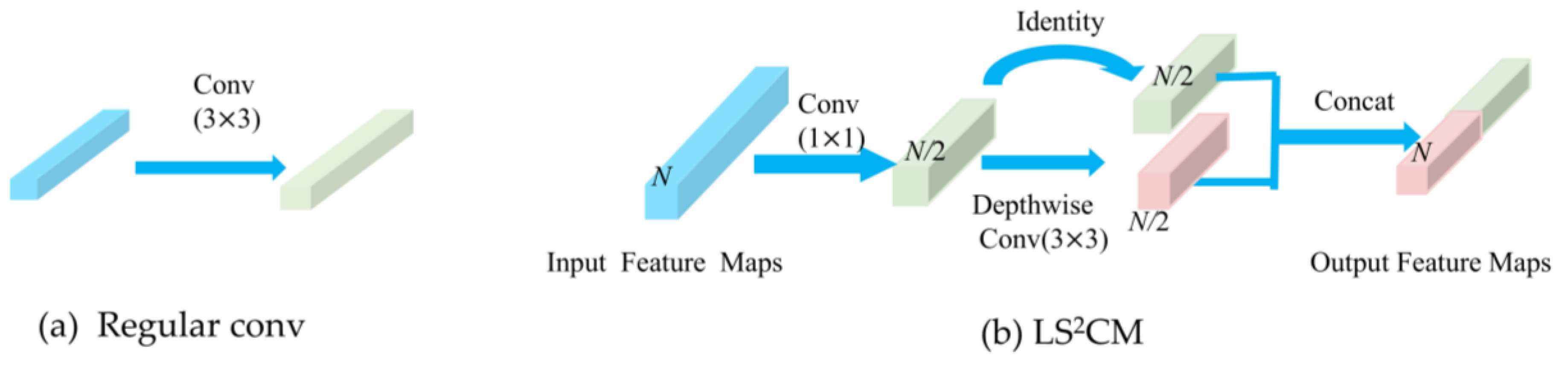
Figure 1.
Differences between a standard convolutional layer (a) and the LS2CM module (b).
Figure 1.
Differences between a standard convolutional layer (a) and the LS2CM module (b).
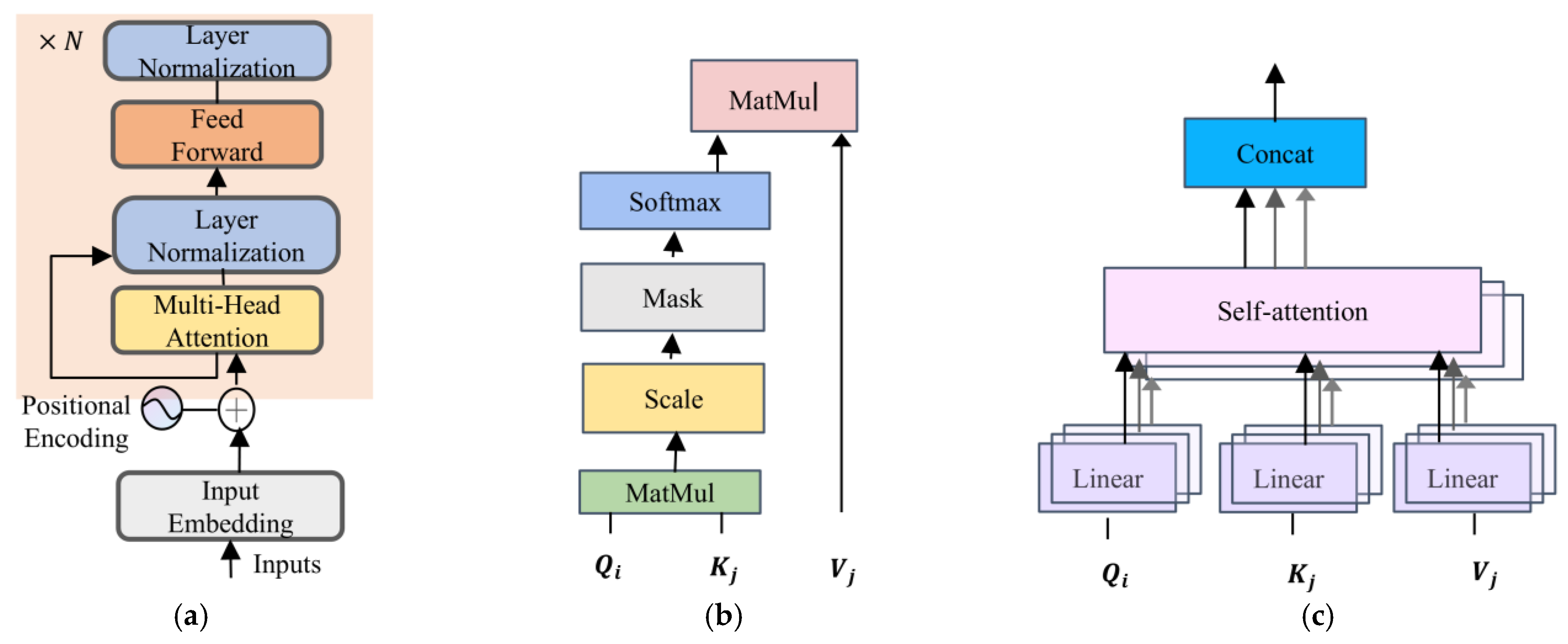
Figure 2.
Transformer encoder components: (a) transformer encoder, (b) self-attention mechanism, and (c) multi-head self-attention.
Figure 2.
Transformer encoder components: (a) transformer encoder, (b) self-attention mechanism, and (c) multi-head self-attention.
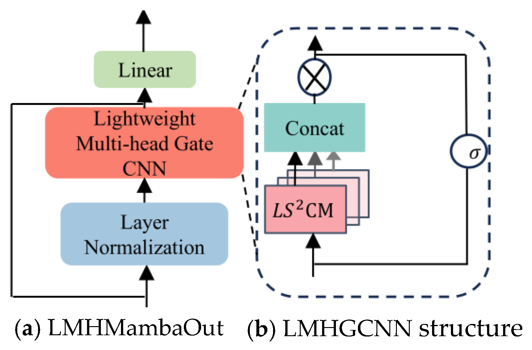
Figure 3.
MambaOut and gated CNN block structures.
Figure 3.
MambaOut and gated CNN block structures.
Figure 4.
The proposed network. HSIs are divided into spatial and spectral branches after PCA preprocessing. The spatial feature extraction module is divided into local spatial feature extraction using the 3D-2D network and global feature extraction using LMHMambaOut. The spectral feature extraction module is divided into local spectral feature extraction using the 3D-2D network and global spectral feature extraction using CosTaylorFormer. After fusing the spatial and spectral features using the dynamic information fusion strategy, they are finally classified through MLP.
Figure 5.
LMHMambaOut structure.
Figure 5.
LMHMambaOut structure.
Figure 6.
Selection of representative plants and crops in the classification of HSI; (a) spectral curves of wood, grass-tree, and corn-no-till; (b) comparison of wood’s spectral characteristics with the Gaussian function; (c) comparison of the Gaussian function and the half-cosine function with amplitudes of 1 within the range of [−4, 4].
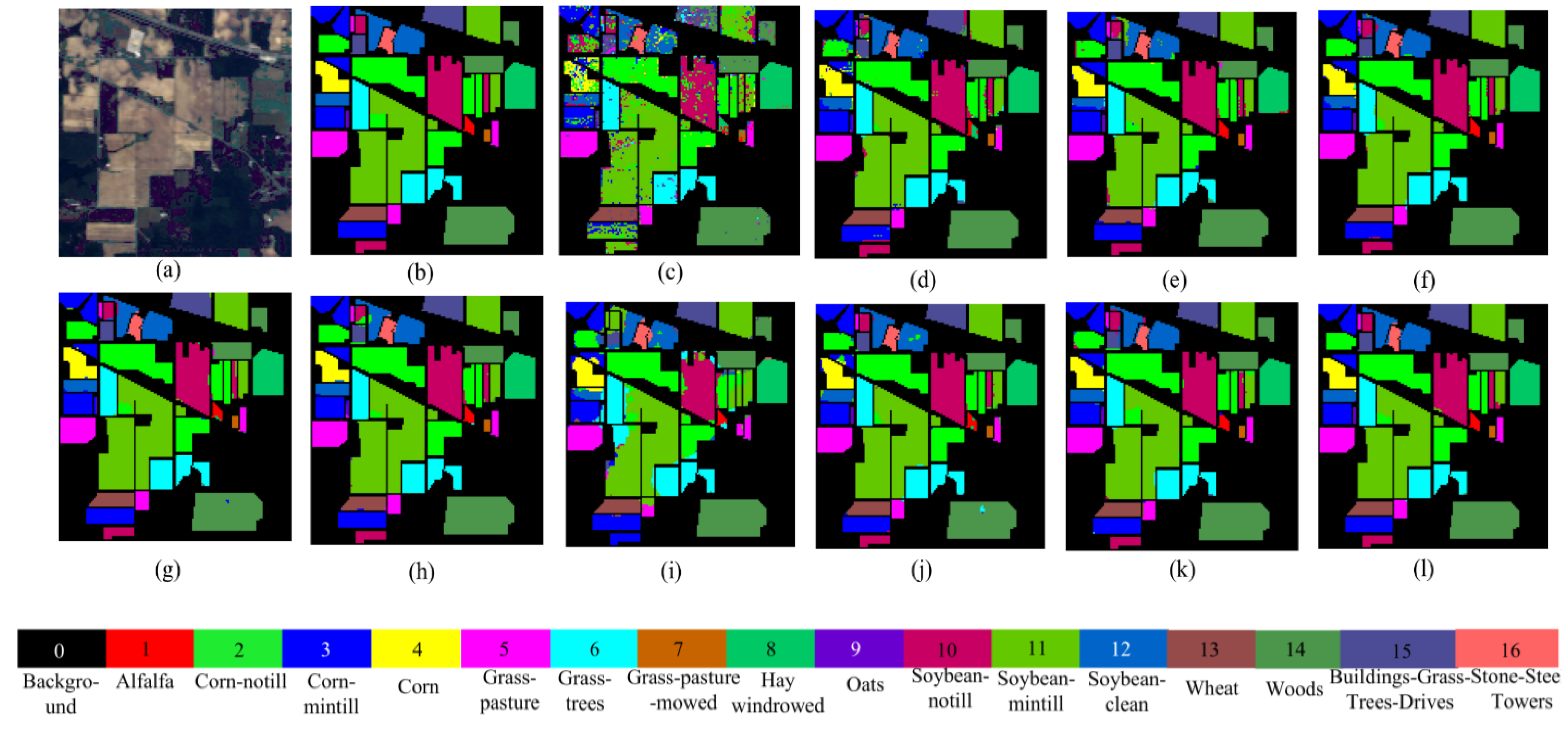
Figure 7.
Visualized classification results of different network models on the IP dataset. (a) False color image of the IP dataset, (b) ground truth, (c) SVM, (d) 2D CNN, (e) HybirdSN, (f) DPResNet, (g) ViT, (h) CTMixer, (i) ResNet-LS2CM, (j) S3EresBof, (k) LSGA-VIT, and (l) proposed network.
Figure 7.
Visualized classification results of different network models on the IP dataset. (a) False color image of the IP dataset, (b) ground truth, (c) SVM, (d) 2D CNN, (e) HybirdSN, (f) DPResNet, (g) ViT, (h) CTMixer, (i) ResNet-LS2CM, (j) S3EresBof, (k) LSGA-VIT, and (l) proposed network.
Figure 8.
Visualized classification results of different network models on the WHU-HI-Longkou dataset. (a) False color image of the SA dataset, (b) ground truth, (c) SVM, (d) 2D CNN, (e) HybirdSN, (f) DPResNet, (g) ViT, (h) CTMixer, (i) ResNet-LS2CM, (j) S3EresBof, (k) LSGA-VIT, and (l) proposed network.
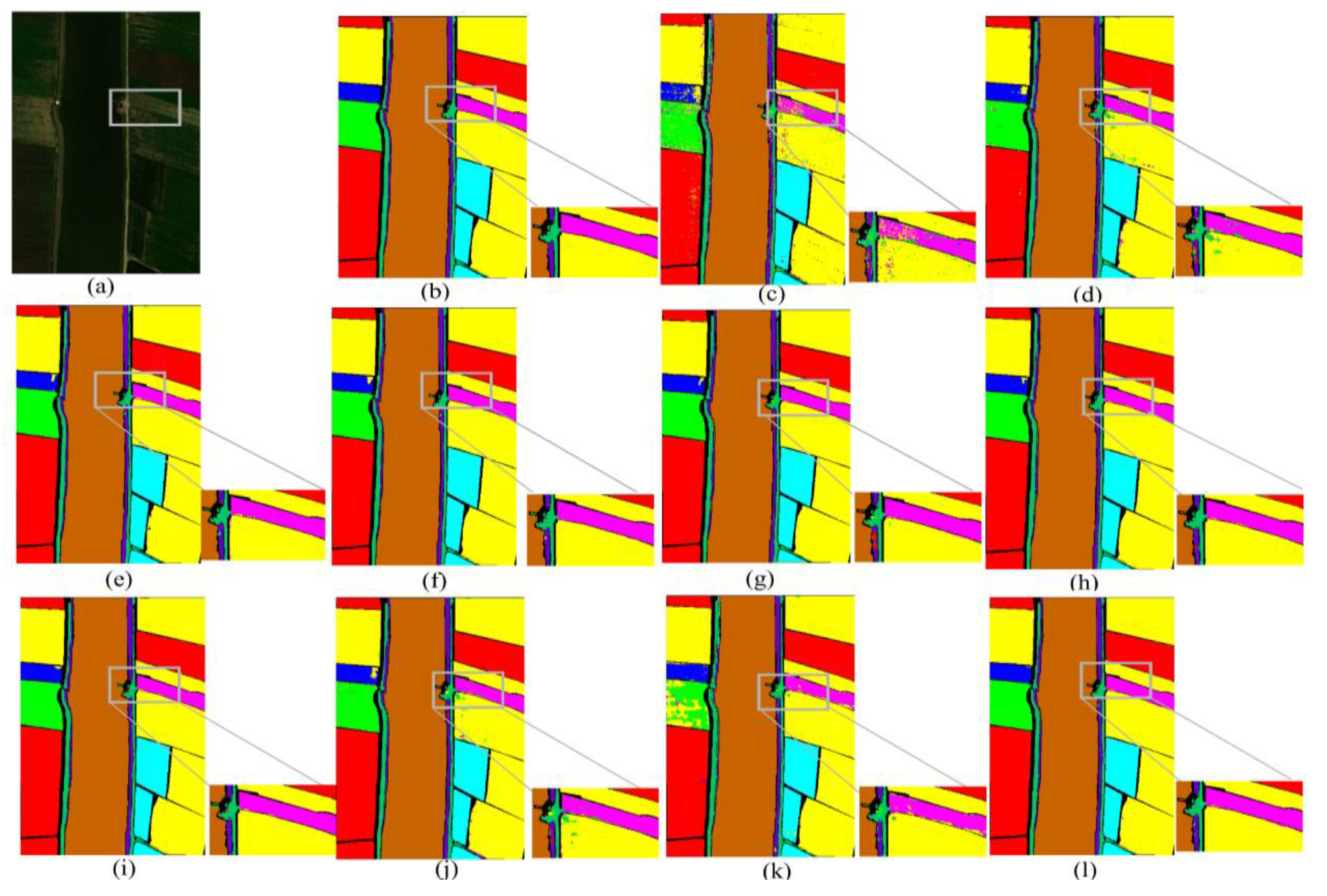
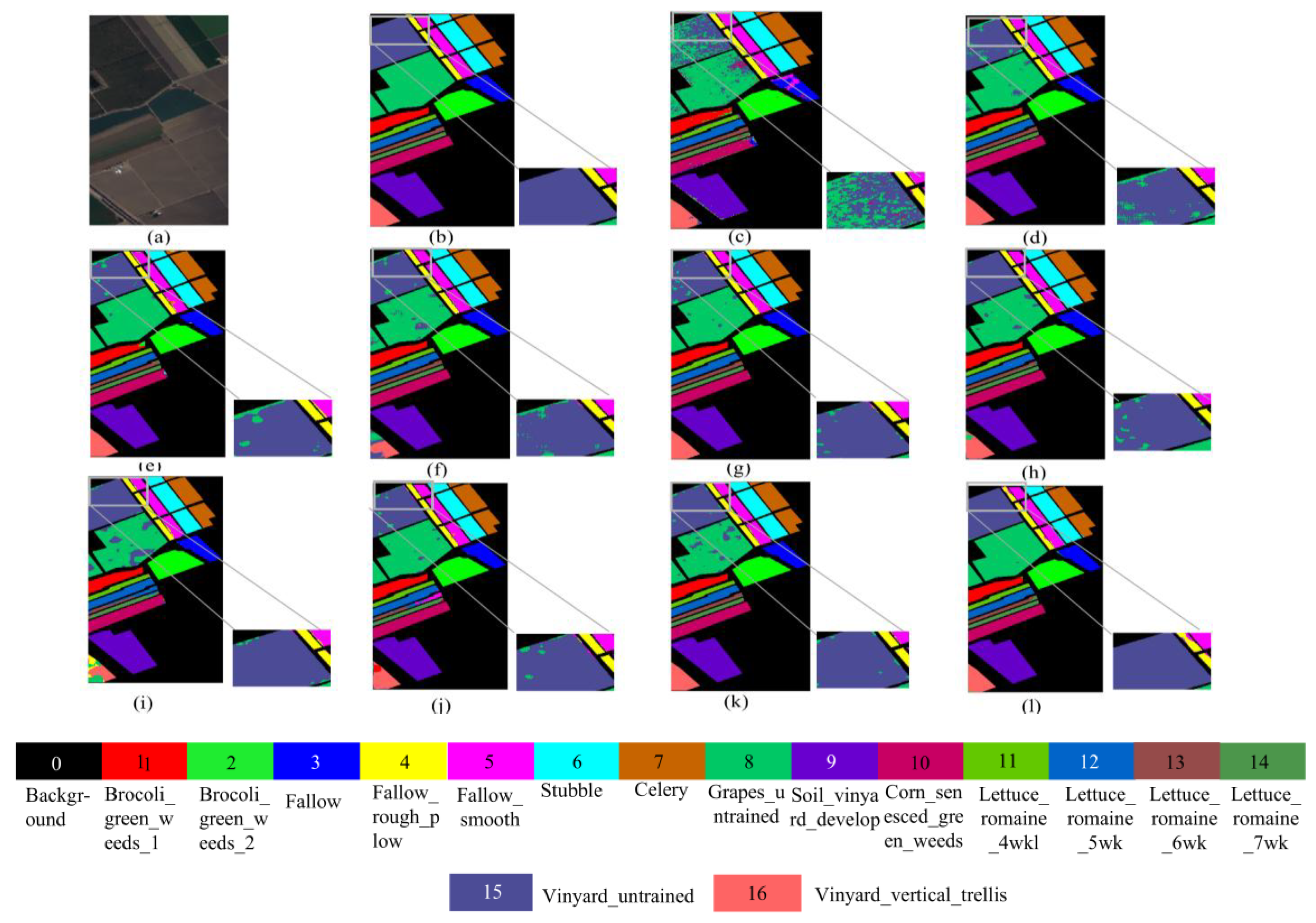
Figure 9.
Visualized classification results of different network models on the SA dataset. (a) False color image of the SA dataset, (b) ground truth, (c) SVM, (d) 2D CNN, (e) HybirdSN, (f) DPResNet, (g) ViT, (h) CTMixer, (i) ResNet-LS2CM, (j) S3EresBof, (k) LSGA-VIT, and (l) proposed network.
Figure 9.
Visualized classification results of different network models on the SA dataset. (a) False color image of the SA dataset, (b) ground truth, (c) SVM, (d) 2D CNN, (e) HybirdSN, (f) DPResNet, (g) ViT, (h) CTMixer, (i) ResNet-LS2CM, (j) S3EresBof, (k) LSGA-VIT, and (l) proposed network.
Figure 10.
Visualized classification results of different network models on the PU dataset. (a) False color image of the PU dataset, (b) ground truth, (c) SVM, (d) 2D CNN, (e) HybirdSN, (f) DPResNet, (g) ViT, (h) CTMixer, (i) ResNet-LS2CM, (j) S3EresBof, (k) LSGA-VIT, and (l) proposed network.
Figure 10.
Visualized classification results of different network models on the PU dataset. (a) False color image of the PU dataset, (b) ground truth, (c) SVM, (d) 2D CNN, (e) HybirdSN, (f) DPResNet, (g) ViT, (h) CTMixer, (i) ResNet-LS2CM, (j) S3EresBof, (k) LSGA-VIT, and (l) proposed network.
Figure 11.
The classification results are subjected to feature extraction using 2D t-SNE. (a) IP dataset, (b) 2D CNN, (c) HybirdSN, (d) DPResNet, (e) ViT, (f) CTMixer, (g) ResNet-LS2CM, (h) S3EresBof, (i) LSGA-VIT, and (j) our proposed network. The different colors from 1 to 16 in the figure represent 16 different categories of the IP dataset.
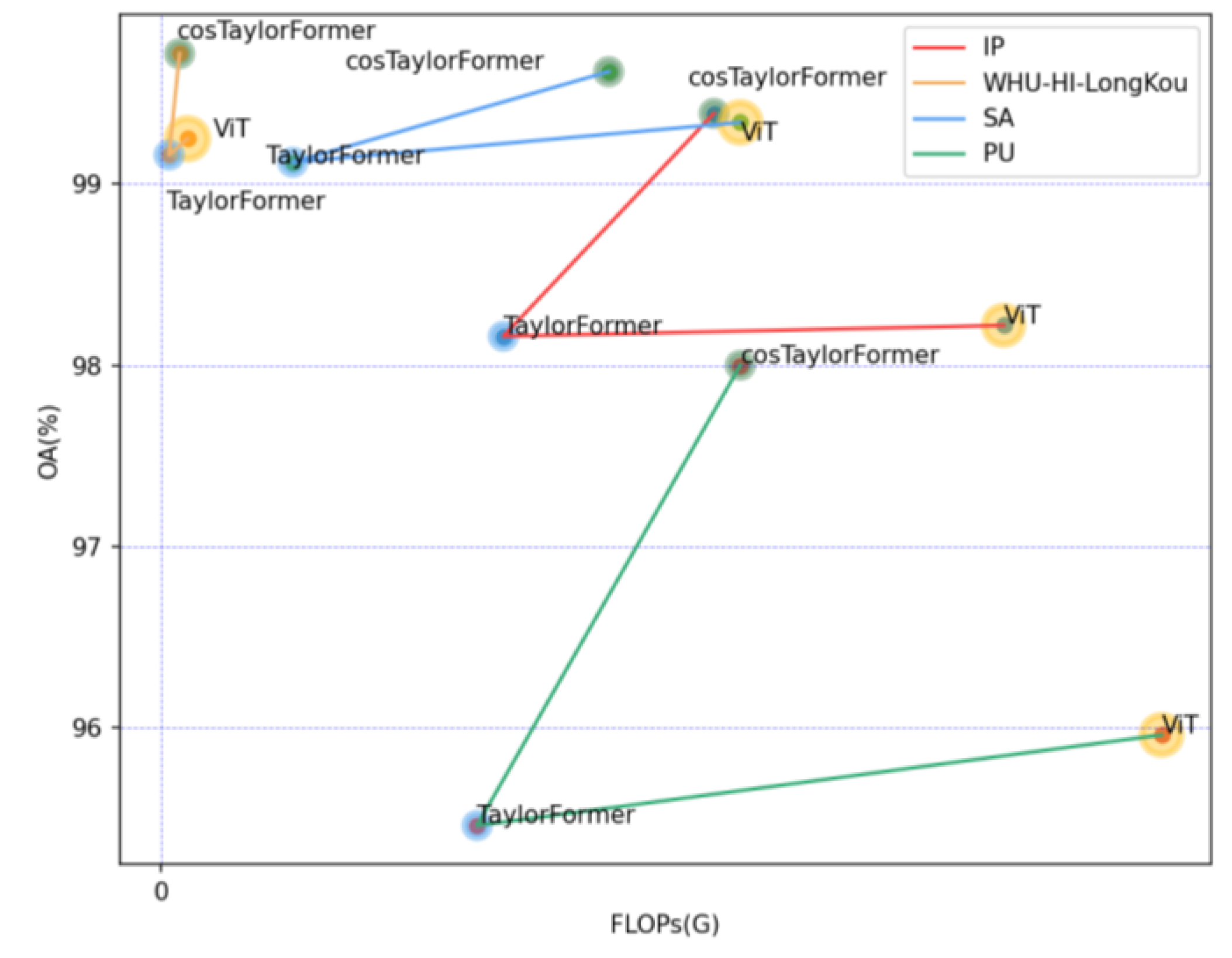
Figure 12.
Verification of the effectiveness of CosTaylorFormer on the IP, WHU-Hi-LongKou, SA, and PU datasets in terms of OA, parameters, and FLOPs. The size of the circle in the figure indicates the number of parameters.
Figure 12.
Verification of the effectiveness of CosTaylorFormer on the IP, WHU-Hi-LongKou, SA, and PU datasets in terms of OA, parameters, and FLOPs. The size of the circle in the figure indicates the number of parameters.
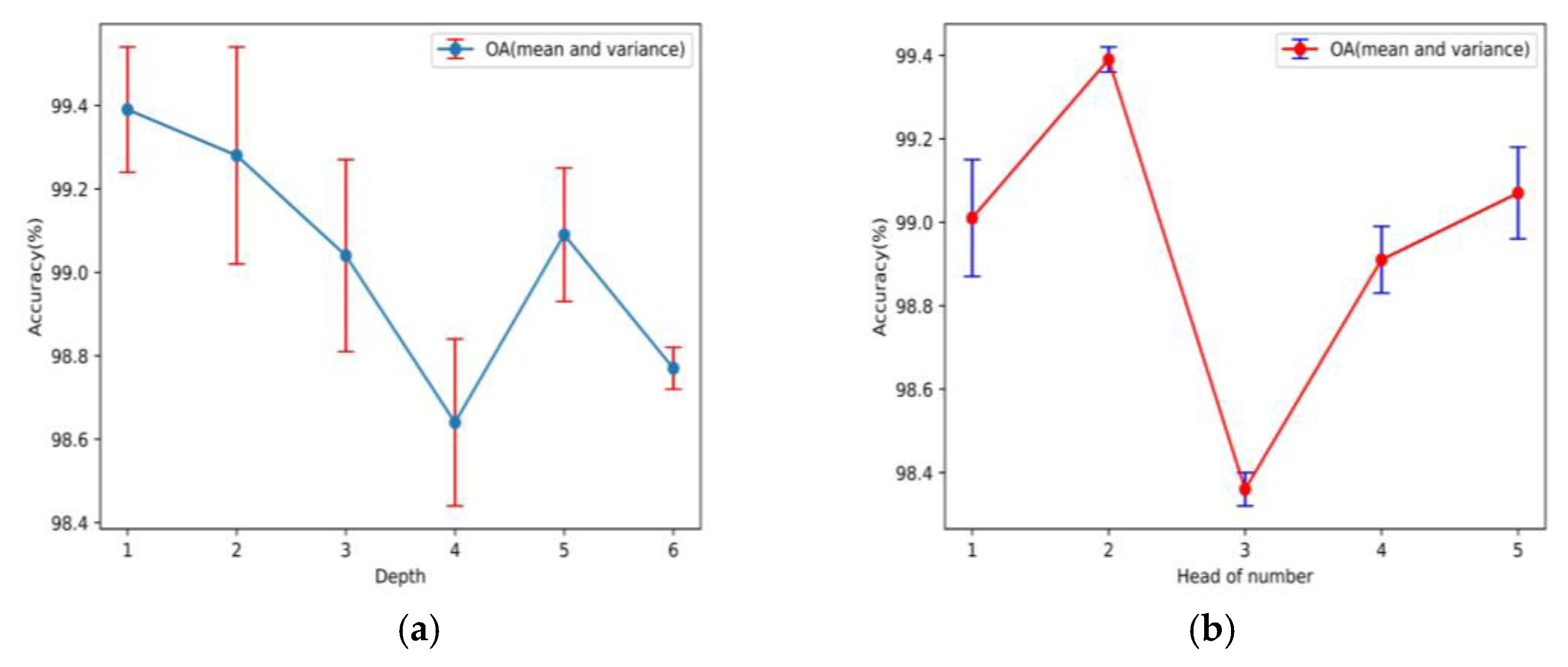
Figure 13.
Optimal parameter settings for depth and number of heads in CosTaylorFormer: (a) the effect of depth on OA and (b) the effect of the number of heads on OA.
Figure 13.
Optimal parameter settings for depth and number of heads in CosTaylorFormer: (a) the effect of depth on OA and (b) the effect of the number of heads on OA.
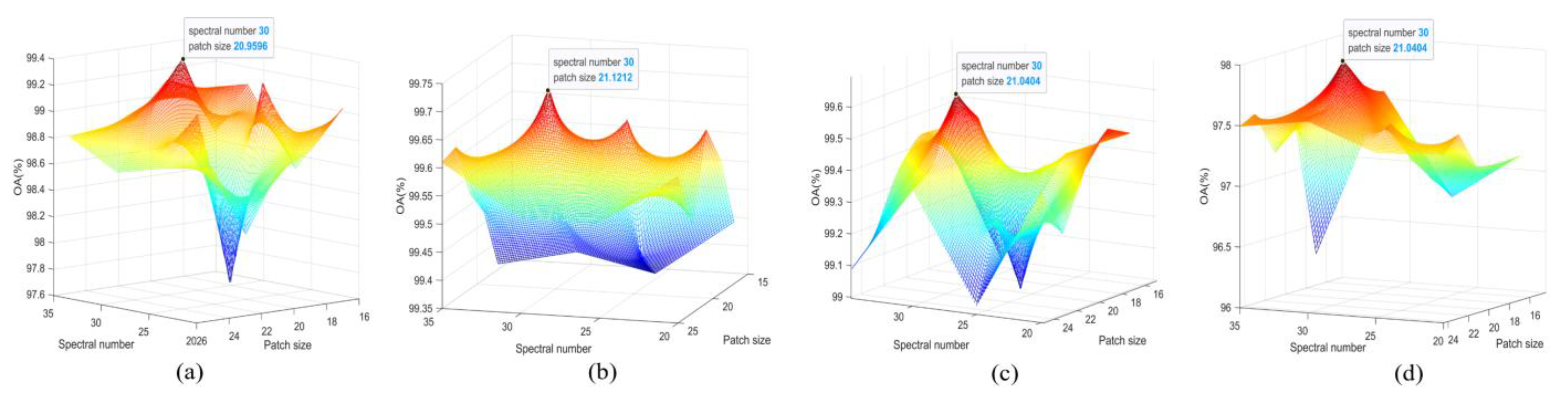
Figure 14.
OA of different patch sizes and spectral dimensions three-dimensional hot spot map on (a) IP, (b) WHU-Hi-LongKou, (c) SA, and (d) PU datasets, with red indicating the maximum.
Figure 14.
OA of different patch sizes and spectral dimensions three-dimensional hot spot map on (a) IP, (b) WHU-Hi-LongKou, (c) SA, and (d) PU datasets, with red indicating the maximum.
Figure 15.
The accuracy trends of 2D CNN, HybirdSN, DPresNet, ResNet-LS2CM, S3EResBof, and our proposed network as a function of training percentage on the IP (a), WHU-Hi-LongKou (b), SA (c), and PU datasets (d). The horizontal axis represents the training percentage, while the vertical axis shows the OA for the current training data.
Table 1.
Specific structure of spatial feature extraction module.
Table 1.
Specific structure of spatial feature extraction module.
| Name | Layer | In_Channels | Out_Channels | Kernel Size | with |
|---|
| 1 | 3D Conv | 1 | 8 | (1, 3, 3) | - |
| 2 | 3D Conv | 8 | 16 | (1, 5, 5) | Relu |
| 3 | 2D Conv | 480 | 60 | (3, 3) | - |
| 4 | LMHMambaOut | 60 | 60 × 4 | (1, 1) (3, 3) (5, 5) | - |
| 6 | LMHMambaOut | 60 | 60 | (1, 1) (3, 3) (5, 5) | - |
Table 2.
Categories and sample sizes of the four datasets.
Table 3.
Classification accuracy and complexity of different networks on the IP dataset.
Table 3.
Classification accuracy and complexity of different networks on the IP dataset.
| Class | Traditional Model | CNN Architecture Network | ViT Architecture Network | Lightweight Network |
|---|
| SVM | 2D-CNN | HybirdSN | DPresNet | ViT | CTMixer | ResNet-LS2CM | S3EresBof | LSGA-VIT | Ours |
|---|
| 1 (Alfalfa) | | 95.00 | 91.71 | | 98.29 | | 58.55 | 98.37 | 92.68 | |
| 2 (Corn-notill) | | 89.77 | 93.18 | 95.71 | 94.17 | 98.52 | 91.29 | 95.45 | 98.46 | 98.67 |
| 3 (Corn-mintill) | | 97.87 | 97.14 | 99.31 | 97.69 | 99.84 | 97.25 | 96.1 | 99.24 | |
| 4 (Corn) | 52.34 | 88.1 | 87.23 | 99.2 | 99.44 | | 92.2 | 99.79 | 96.34 | |
| 5 (Grasspasture) | 92.88 | 90.93 | 98.94 | 98.62 | 99.15 | | 93.79 | 98.24 | 97.88 | |
| 6 (Grass-trees) | 95.89 | 100 | 99.1 | 99 | 99.33 | 99.65 | 97.87 | 96.57 | 98.11 | |
| 7 (Grass-pasture-mowed) | 65.38 | | 99.2 | | 99.11 | | 29.2 | 87.87 | | |
| 8 (Hay-windrowed) | 98.61 | | 99.95 | | 1000 | | 99.98 | 99.48 | 99.81 | |
| 9 (Oats) | 33.33 | 50.00 | 96.55 | 92.77 | 81.11 | 75.00 | 33.89 | | 98.89 | 90.00 |
| 10 (Soybean-notill) | 68.22 | 97.70 | 97.96 | 98.48 | 96.31 | 99.39 | 94.24 | 97.12 | 99.46 | |
| 11 (Soybean-mintill) | 83.07 | 98.64 | 98.61 | 99.36 | 99.16 | 99.18 | 97.36 | 96.41 | 98.66 | |
| 12 (Soybean-clean) | 68.35 | 87.74 | 90.05 | 96.08 | 95.67 | 97.92 | 85.38 | 95.96 | 95.28 | |
| 13 (Wheat) | 95.14 | 94.74 | 99.02 | 98.91 | 98.38 | | 97.51 | 97.77 | | 99.47 |
| 14 (Woods) | 96.66 | | 99.73 | 99.9 | 99.73 | | 99.38 | 97.08 | | |
| 15 (Buildings-Grass-Trees-Drives) | 54.59 | 99.43 | 98.44 | 99.8 | 98.88 | 99.71 | 95.13 | 95.14 | 97.03 | |
| 16 (Stone-Steel-Towers) | 94.05 | | 94.05 | 95.59 | 56.31 | 98.75 | 91.19 | 93.92 | 87.97 | 92.5 |
| OA | 80.09 | 95.9 | 97.09 | 98.58 | 97.52 | 99.24 | 95.02 | 96.69 | 98.49 | |
| AA | 72.64 | 93.12 | 96.24 | 98.3 | 93.93 | 98.07 | 84.63 | 96.74 | 97.49 | |
| Kappa | 77.19 | 95.67 | 96.68 | 98.38 | 97.16 | 99.31 | 94.28 | 96.23 | 98.29 | |
| Parameter/M | — | 1.05 | 9.01 | 1.86 | 0.31 | 0.63 | 0.01 | 0.23 | 0.54 | 0.22 |
| Training time (s) | — | 27.96 | 53.39 | 128.03 | 25.46 | 256.90 | 9.08 | 15.84 | 36.12 | 15.15 |
| Test time (s) | — | 0.27 | 0.72 | 37.52 | 0.78 | 0.20 | 0.23 | 1.73 | 0.46 | 0.17 |
| FLOPs/G | — | 0.11 | 0.55 | 2.93 | 0.88 | 2.01 | 0.45 | 0.62 | 0.41 | 0.32 |
Table 4.
Classification accuracy and complexity of different networks on the WHU-Hi-LongKou dataset.
Table 4.
Classification accuracy and complexity of different networks on the WHU-Hi-LongKou dataset.
| Class | Traditional Model | CNN Architecture Network | ViT Architecture Network | Lightweight Network |
|---|
| SVM | 2D-CNN | HybirdSN | DpresNet | ViT | CTMixer | ResNet-LS2CM | S3EresBof | LSGA-VIT | Ours |
|---|
| 1 (Corn) | 98.81 | 99.96 | 99.86 | 99.97 | 99.79 | | 99.92 | 99.82 | 99.89 | |
| 2 (Cotton) | 86.99 | 96.86 | 98.92 | 99.75 | 99.67 | 99.83 | 99.6 | 99.37 | 99.69 | |
| 3 (Sesame) | 77.51 | 92.81 | 94.43 | 96.59 | 96.53 | 99.74 | 96.11 | | 98.76 | |
| 4 (Broad-leaf soybean) | 97.62 | 98.86 | 99.18 | 99.82 | 99.76 | 99.75 | 99.71 | 99.26 | 99.68 | |
| 5 (Narrow-leaf soybean) | 75.54 | 94.54 | 97.84 | 98.75 | 99.02 | 98.02 | 98.46 | 99.63 | 98.76 | |
| 6 (Rice) | 99.13 | 99.54 | 99.4 | 99.67 | 99.04 | | 99.52 | 99.04 | 99.58 | 99.86 |
| 7 (Water) | 99.93 | 99.950.04 | 99.83 | 99.96 | 99.79 | | 99.89 | 99.91 | 99.91 | 99.95 |
| 8 (Roads and houses) | 87.39 | 96.86 | 97.69 | 96.88 | 96.45 | 96.78 | 95.66 | 92.3 | 96.50 | |
| 9 (Mixed weed) | 81.23 | 93.05 | 92.34 | 95.28 | 92.59 | | 91.07 | 97.6 | 94.46 | 95.28 |
| OA | 96.71 | 98.97 | 99.18 | 99.59 | 99.38 | 99.64 | 99.35 | 99.06 | 99.51 | |
| AA | 89.34 | 96.94 | 97.72 | 98.52 | 98.08 | 98.92 | 97.77 | 98.55 | 98.58 | |
| Kappa | 95.66 | 98.64 | 98.94 | 99.46 | 99.19 | 99.53 | 99.15 | 99.06 | 99.36 | |
| parameter/M | — | 1.05 | 1.69 | 1.86 | 0.54 | 0.63 | 0.01 | 0.24 | 0.23 | 0.22 |
| Training time (s) | — | 11.72 | 35.47 | 48.21 | 38.25 | 78.24 | 24.73 | 25.80 | 20.48 | 20.23 |
| Test time (s) | — | 3.03 | 6.61 | 4.85 | 7.71 | 7.14 | 6.17 | 6.51 | 6.22 | 5.17 |
| FLOPs/G | — | 2.93 | 12.68 | 40.02 | 3.05 | 31.54 | 1.01 | 2.35 | 1.11 | 2.22 |
Table 5.
Classification accuracy and complexity of different networks on the SA dataset.
Table 5.
Classification accuracy and complexity of different networks on the SA dataset.
| Class | Traditional Model | CNN Architecture Network | ViT Architecture Network | Lightweight Network |
|---|
| SVM | 2D-CNN | HybirdSN | DpresNet | ViT | CTMixer | ResNet-LS2CM | S3EresBof | LSGA-VIT | Ours |
|---|
| 1 (Brocoli_green_weeds_1) | 96.62 | 99.81 | 99.95 | 98.51 | 100 | 99.98 | 99.22 | 99.69 | 99.99 | |
| 2 (Brocoli_green_weeds_2) | 99.27 | 100 | 100 | 99.8 | 100 | 100 | 99.96 | 99.93 | 99.89 | |
| 3 (Fallow) | 95.62 | 98.4 | 99.38 | 99.87 | | 99.99 | 99.9 | 99.96 | 99.99 | |
| 4 (Fallow_rough_plow) | 98.92 | 99.00 | 98.31 | 99.33 | 99.53 | 99.83 | 98.6 | 97.88 | | 99.52 |
| 5 (Fallow_smooth) | 94.86 | 98.77 | 98.22 | 95.9 | 98.95 | 99.15 | 98.27 | 97.51 | | 98.68 |
| 6 (Stubble) | 99.36 | 99.74 | 99.93 | 99.7 | 99.74 | 99.97 | 99.89 | 99.83 | | |
| 7 (Celery) | 99.43 | 99.96 | 99.83 | 99.51 | 99.78 | 99.81 | 99.53 | 99.82 | | |
| 8 (Grapes_untrained) | 89.18 | 97.360.95 | 96.78 | 97.91 | 98.03 | 97.06 | 97.72 | 97.57 | 94.76 | |
| 9 (Soil_vinyard_develop) | 98.62 | 100 | 99.99 | 99.98 | 100 | 100 | 99.96 | 99.85 | | |
| 10 (Corn_senesced_green_weeds) | 87.00 | 99.15 | 99.18 | 98.8 | | 98.97 | 98.74 | 99.13 | 98.72 | 99.26 |
| 11 (Lettuce_romaine_4wk) | 90.34 | 98.58 | 99.1 | 99.06 | 99.44 | 99.53 | 99.54 | 99.89 | | |
| 12 (Lettuce_romaine_5wk) | 98.83 | 98.69 | 99.57 | 97.46 | | 99.85 | 98.29 | 98.69 | 99.61 | 99.71 |
| 13 (Lettuce_romaine_6wk) | | 94.50 | 97.95 | 90.32 | 92.34 | 95.18 | 70.91 | 87.76 | 95.37 | |
| 14 (Lettuce_romaine_7wk) | 91.8 | 96.58 | 98.94 | 96.27 | 98.86 | 98.33 | 93.5 | 92.29 | | 98.83 |
| 15 (Vinyard_untrained) | 50.33 | 93.34 | 88.81 | 96.05 | 95.19 | 98.17 | 94.33 | 97.33 | 96.45 | |
| 16 (Vinyard_vertical_trellis) | 94.96 | 99.72 | 99.22 | 98.61 | 99.32 | 99.8 | 99.26 | 99.65 | 99.65 | |
| OA | 88.92 | 98.08 | 97.49 | 97.98 | 98.62 | 98.88 | 97.77 | 98.34 | 98.21 | |
| AA | 92.72 | 98.35 | 98.45 | 98.03 | 98.8 | 99.1 | 96.73 | 97.92 | 99.05 | |
| Kappa | 87.62 | 97.86 | 97.2 | 97.75 | 98.46 | 98.76 | 97.52 | 98.15 | 98.01 | |
| parameter/M | — | 1.05 | 3.70 | 1.86 | 0.27 | 0.63 | 0.01 | 0.24 | 0.54 | 0.22 |
| Training time (s) | — | 10.77 | 16.12 | 16.81 | 11.67 | 44.33 | 13.91 | 18.41 | 26.12 | 13.78 |
| Test time (s) | — | 2.34 | 1.90 | 6.66 | 1.73 | 4.24 | 1.45 | 7.28 | 2.46 | 1.17 |
| FLOPs/G | — | 0.33 | 2.25 | 47.61 | 1.40 | 11.54 | 1.18 | 3.20 | 2.45 | 2.15 |
Table 6.
Classification accuracy and complexity of different networks on the PU dataset.
Table 6.
Classification accuracy and complexity of different networks on the PU dataset.
| Class | Traditional Model | CNN Architecture Network | ViT Architecture Network | Lightweight Network |
|---|
| SVM | 2D-CNN | HybirdSN | DpresNet | ViT | CTMixer | ResNet-LS2CM | S3EresBof | LSGA-VIT | Ours |
|---|
| 1 (Alfalfa) | | | | | | | | | | |
| 2 (Meadows) | | | | | | | | | | |
| 3 (Gravel) | | | | | | | | | | |
| 4 (Trees) | | | | | | | | | | |
| 5 (Painted metal sheets) | | | | | | | | | | |
| 6 (Bare Soil) | | | | | | | | | | |
| 7 (Bitumen) | | | | | | | | | | |
| 8 (Self-Blocking Bricks) | | | | | | | | | | |
| 9 (Shadows) | | | | | | | | | | |
| OA | | | | | | | | | | |
| AA | | | | | | | | | | |
| Kappa | | | | | | | | | | |
| parameter/M | — | 1.05 | 1.71 | 1.86 | 0.27 | 0.63 | 0.01 | 0.24 | 0.54 | 0.22 |
| Training time (s) | — | 2.96 | 3.38 | 15.18 | 6.39 | 39.38 | 10.75 | 18.95 | 36.12 | 2.07 |
| Test time (s) | — | 0.46 | 9.91 | 5.11 | 1.06 | 11.87 | 1.28 | 6.28 | 0.46 | 0.43 |
| FLOPs/G | — | 0.32 | 1.38 | 28.10 | 1.17 | 25.93 | 5.37 | 15.27 | 2.45 | 1.06 |
Table 7.
Model complexity comparison.
Table 7.
Model complexity comparison.
| Model | 2D-CNN | HybirdSN | DPresNet | ViT | CTMixer | ResNet-LS2CM | S3EresBof | LSGA-VIT | Ours |
|---|
| Paramparas/M | 1.05 | 9.01 | 1.86 | 0.31 | 0.63 | 0.01 | 0.23 | 0.54 | 0.22 |
| Training time (s) | 27.96 | 53.39 | 128.03 | 25.46 | 256.90 | 9.08 | 15.84 | 36.12 | 15.15 |
| Test time (s) | 0.27 | 0.72 | 37.52 | 0.78 | 0.20 | 0.23 | 1.73 | 0.46 | 0.17 |
| FLOPs/G | 0.11 | 0.55 | 2.93 | 0.88 | 2.01 | 0.45 | 0.62 | 0.41 | 0.32 |
Table 8.
Verification of the effectiveness of LMHMambaOut, CosTaylorFormer, and DIFS on the IP, WHU-Hi-LongKou, SA, and PU datasets.
Table 8.
Verification of the effectiveness of LMHMambaOut, CosTaylorFormer, and DIFS on the IP, WHU-Hi-LongKou, SA, and PU datasets.
| Data | Model | OA | AA | Kappa | Parameter/M | FLOPs/G |
|---|
| IP | Baseline | | | | 0.47 | 0.02 |
| Baseline + LMHMambaOut | | | | 0.60 | 0.30 |
| Baseline + LMHMambaOut + CosTaylorformer | | | | 0.22 | 0.32 |
| Baseline + LMHMambaOut + CosTaylorformer + DIFS | | | | 0.22 | 0.32 |
| WHU-HI-Longkou | Baseline | 96.62 ± 0.01 | 94.29 ± 0.13 | 95.36 ± 0.13 | 0.47 | 0.08 |
| Baseline + LMHMambaOut | | | | 0.60 | 1.46 |
| Baseline + LMHMambaOut + CosTaylorformer | 99.53 | 98.54 | 99.38 | 0.22 | 2.22 |
| Baseline + LMHMambaOut + CosTaylorformer + DIFS | | | | 0.22 | 2.22 |
| SA | Baseline | | | | 0.47 | 0.86 |
| Baseline + LMHMambaOut | | | | 0.60 | 1.58 |
| Baseline + LMHMambaOut + CosTaylorformer | 99.30 | 98.83 | 99.22 | 0.22 | 2.15 |
| Baseline + LMHMambaOut + CosTaylorformer + DIFS | | | | 0.22 | 2.15 |
| PU | Baseline | | | | 0.47 | 0.52 |
| Baseline + LMHMambaOut | | | | 0.60 | 0.91 |
| Baseline + LMHMambaOut + CosTaylorformer | 97.21 | 95.05 | 96.31 | 0.22 | 1.06 |
| Baseline + LMHMambaOut + CosTaylorformer + DIFS | | | | 0.22 | 1.06 |
Table 9.
Comparison of classification accuracy: dynamic information fusion strategy vs. concatenation and addition operations.
Table 9.
Comparison of classification accuracy: dynamic information fusion strategy vs. concatenation and addition operations.
| Data | Operation | OA | AA | Kappa |
|---|
| IP | Concat | 99.03 | 98.70 | 98.89 |
| Add | 98.94 | 97.72 | 98.80 |
| Dynamic information fusion strategy | 99.39 | 99.19 | 99.31 |
| WHU-Hi-LongKou | Concat | 99.54 | 98.45 | 99.39 |
| Add | 99.53 | 98.54 | 99.38 |
| Dynamic information fusion strategy | 99.72 | 99.02 | 99.63 |
| SA | Concat | 99.55 | 99.19 | 99.51 |
| Add | 99.30 | 98.83 | 99.22 |
| Dynamic information fusion strategy | 99.62 | 99.3 | 99.58 |
| PU | Concat | 97.07 | 95.42 | 96.11 |
| Add | 97.21 | 95.05 | 96.31 |
| Dynamic information fusion strategy | 97.30 | 93.61 | 96.42 |


