Retrieving Inland Water Quality Parameters via Satellite Remote Sensing: Sensor Evaluation, Atmospheric Correction, and Machine Learning Approaches

Ansari, Mohsen; Knudby, Anders; Amani, Meisam; Sawada, Michael

doi:10.3390/rs17101734

Open AccessReview

Retrieving Inland Water Quality Parameters via Satellite Remote Sensing: Sensor Evaluation, Atmospheric Correction, and Machine Learning Approaches

¹

Department of Geography, Environment and Geomatics, University of Ottawa, 75 Laurier Avenue East, Ottawa, ON K1N 6N5, Canada

²

Canada Centre for Mapping and Earth Observation, Natural Resources Canada, 560 Rochester Street, Ottawa, ON K1S 4M2, Canada

^*

Author to whom correspondence should be addressed.

Remote Sens. 2025, 17(10), 1734; https://doi.org/10.3390/rs17101734

Submission received: 10 April 2025 / Revised: 10 May 2025 / Accepted: 12 May 2025 / Published: 15 May 2025

(This article belongs to the Special Issue River and Lake Dynamic Monitoring and Ecological Assessment Based on Remote Sensing)

Download

Browse Figures

Review Reports Versions Notes

Abstract

:

Satellite remote sensing provides a cost-effective and large-scale alternative to traditional methods for retrieving water quality parameters for inland waters. Effective water quality parameter retrieval via optical satellite remote sensing requires three key components: (1) a sensor whose measurements are sensitive to variations in water quality; (2) accurate atmospheric correction to eliminate the effect of absorption and scattering in the atmosphere and retrieve the water-leaving radiance/reflectance; and (3) a bio-optical model used to estimate water quality from the optical signal. This study provides a literature review and an evaluation of these three components. First, a review of decommissioned, active, and upcoming satellite sensors is presented, highlighting their advantages and limitations, and a ranking method is introduced to assess their suitability for retrieving chlorophyll-a, colored dissolved organic matter, and non-algal particles in inland waters. This ranking can aid in selecting appropriate sensors for future studies. Second, the strengths and weaknesses of atmospheric correction algorithms used over inland waters are examined. The results show that no atmospheric correction algorithm performed consistently across all conditions. However, understanding their strengths and weaknesses allows users to select the most suitable algorithm for a specific use case. Third, the challenges, limitations, and recent advances of machine learning use in bio-optical models for inland water quality parameter retrieval are discussed. Machine learning models have limitations, including low generalizability, low dimensionality, spatial/temporal autocorrelation, and information leakage. These issues highlight the importance of locally trained models, rigorous cross-validation methods, and integrating auxiliary data to enhance dimensionality. Finally, recommendations for promising research directions are provided.

Keywords:

satellite remote sensing; inland water quality parameters; water quality retrieval; machine learning models; atmospheric correction; bio-optical methods

1. Introduction

Limnology, the study of inland waters, focuses on the 1% of the Earth’s surface covered by lakes, rivers, wetlands, and other inland water bodies [1]. Inland waters are crucial for biogeochemical cycles, ecology, and human history [2,3]. However, only 60% of known inland waters meet good ambient water quality standards, based on five Water Quality Parameters (WQPs): oxygen, salinity, nitrogen, phosphorus, and acidity [4]. This finding underscores the need for sustainable management of WQPs. Additionally, the risk of water crises, including the decline in freshwater quality, is a global and regional concern [5]. For example, water crises are widely evident in countries like the United States [6], Iran [7], and even Brazil [8], which has the world’s largest supply of freshwater.

Inland waters also act as indicators of environmental change, including climate change [9], land use changes [10], and pollution [11], all of which can lead to harmful impacts such as eutrophication [12]. One of the key challenges in environmental resource management is low-cost enforcement and monitoring [13]. Remote Sensing (RS) offers cost-effective, large-scale, and frequent observations compared to traditional WQP monitoring methods. Given the importance of mapping and monitoring WQPs in inland waters and the advantages of RS methods, as well as the diverse methodologies available, research on retrieving inland WQPs using RS has gained increasing attention (Figure 1).

WQPs can be categorized into three groups: (1) physical parameters, such as temperature, turbidity, Secchi disk depth, salinity, and concentrations of Total Suspended Matter (TSM) or Total Suspended Solids (TSSs), (2) chemical parameters, such as pH and concentrations of Total Dissolved Solid (TDS), nitrogen, Colored Dissolved Organic Matter (CDOM), and phosphorus, and (3) biological parameters, such as concentrations of Chlorophyll-a (Chl-a) and total bacteria. RS methods are used to monitor these WQPs by detecting the optical properties of WQPs. These optical properties are divided into two categories: (1) Apparent Optical Properties (AOPs), which depend on the light field, and (2) Inherent Optical Properties (IOPs), which are independent of the light field.

Accurately monitoring inland WQPs using satellite sensors necessitates a sensor with the following five characteristics:

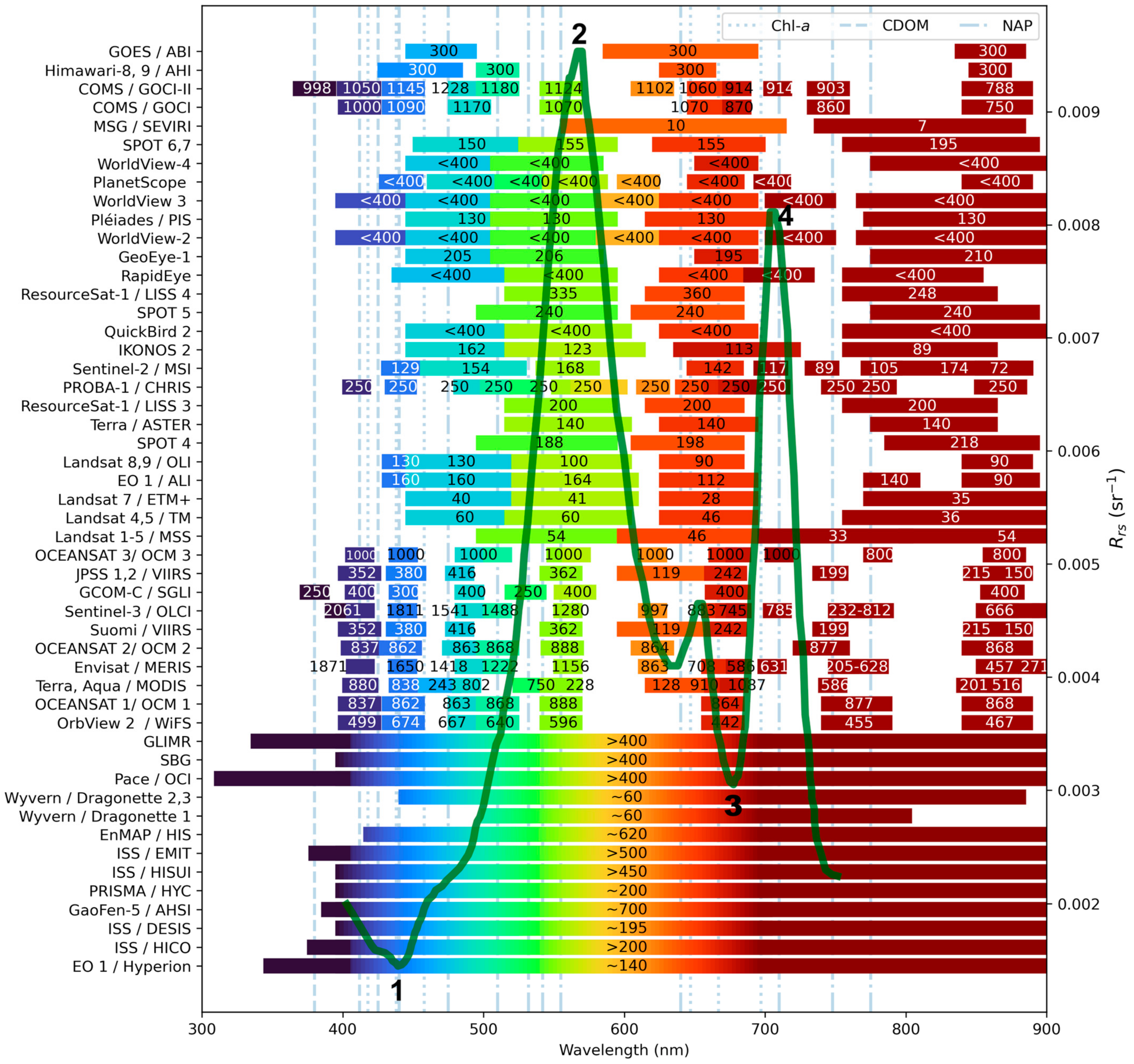
A spatial resolution sufficient for the size of the targeted inland water bodies, which vary from large lakes to narrow rivers;
A high radiometric sensitivity and Signal-to-Noise Ratio (SNR) to capture weak water-leaving radiance/reflectance;
Spectral bands that are sensitive to variations in WQPs;
Frequent temporal coverage to capture the dynamic nature of inland waters;
Design features such as a tilting mechanism to minimize sun glint effects (the specular reflection of direct sunlight from the water surface [14]).

However, due to operational limitations, no single sensor currently meets all these requirements. Reviewing past, present, and upcoming sensors will help determine which sensors meet these requirements and to what extent. Such an evaluation also highlights the potential for combining complementary sensors, enabling the integration of multi-sensor data. This multi-sensor integration approach can enhance inland water monitoring by providing higher temporal [15] or spatial resolution [16] observations compared to those obtained from a single sensor.

The radiance captured at the Top of Atmosphere (TOA) by sensors is affected by atmospheric attenuation and surface reflection at the air–water interface, making robust Atmospheric Correction (AC) essential to mitigate these effects and to enable accurate retrieval of remote sensing reflectance (R_rs) and in turn WQPs from satellite data. While AC methods for open ocean waters are well established [17], additional challenges exist for AC over inland waters. These challenges include the influence of atmospheric aerosols from urban pollution, high turbidity, and the Adjacency Effect (AE) [3,18], leading to uncertainties in WQP modeling. Several AC algorithms have thus been developed for retrieving inland WQPs, each with their own strengths and limitations.

Bio-optical models [19] describe the relationship between optical properties and water constituents and can be classified as physics-based models (e.g., analytical models) and empirical models (including machine learning (ML) models). Physics-based models work by inverting radiative transfer models based on mechanistic principles. They offer physical interpretations and require several parameters like attenuation coefficients of optically active WQPs (e.g., Chl-a, NAP, and CDOM). Physics-based approaches only model optically active WQPs. This is because non-optically active WQPs (e.g., concentrations of TDS, nitrogen, and phosphorus), do not directly affect the attenuation of light in water [20,21]. As a result, non-optically active WQPs cannot be modeled with radiative transfer models.

Empirical models, which are typically based on correlations between in situ measurements of WQPs and radiometric data from satellite sensors, can estimate both optically active and non-optically active WQPs [20]. For non-optically active WQPs, modeling can be performed explicitly by indirectly estimating them from satellite-derived optically active WQPs [22,23]. Alternatively, it can be carried out implicitly, assuming that non-optically active WQPs do not attenuate light in the visible spectrum but still influence the overall optical characteristics of water through correlations with optically active WQPs [20,21]. Empirical models are widely used in inland WQP studies [24] and have surpassed physics-based models in publication volume in recent years (Figure 1). Among empirical models, ML models have become the most popular approach for retrieving WQPs in inland waters (Figure 1). However, the performance of ML models depends on the quality, quantity, and dimensionality of the input data. They may be prone to overfitting if the dataset is insufficient or if overfitting prevention techniques [25,26]—such as cross-validation and regularization—are not properly applied. Additionally, ML models do not inherently incorporate physical principles; instead, they infer patterns from data that may implicitly reflect such principles [27]. Consequently, they are vulnerable to spatial and temporal autocorrelation issues and often exhibit limited generalizability [28,29].

This paper provides a comprehensive and up-to-date overview of past, present, and future satellite sensors capable of retrieving inland WQPs, evaluating their suitability for retrieving optically active WQPs (Section 3). It also explores AC algorithms used in the context of monitoring inland WQPs (Section 4). Furthermore, it discusses the strengths and challenges of ML models for retrieving inland WQPs (e.g., generalizability, spatial and temporal autocorrelation between the data used for training and/or testing, and data dimensionality) and recent methods to address these challenges (Section 5). The review is limited in scope; it is not a meta-analysis, and it does not address the integration of in situ field data with WQP monitoring, nor does it provide a practical evaluation of AC algorithms or bio-optical models through direct implementation and comparison.

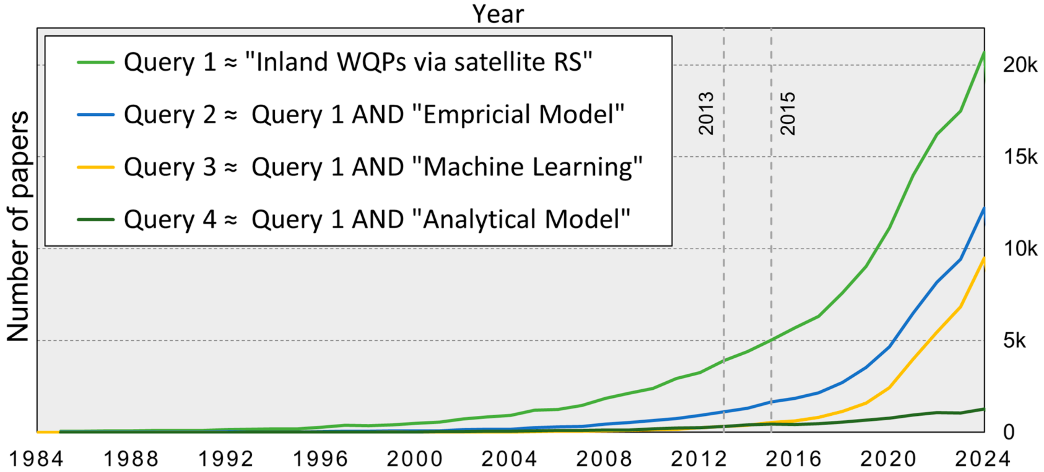
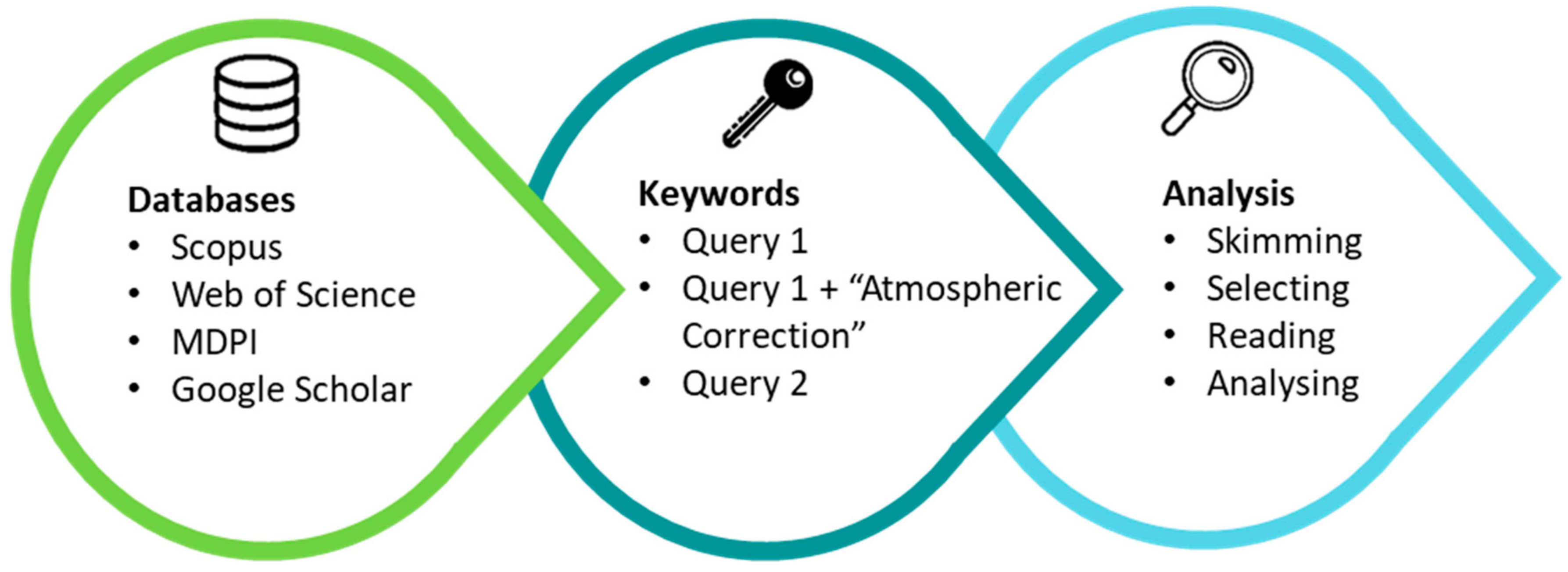
2. Methodology for Article Selection and Filtering

Articles were selected for inclusion in this review using a multi-stage process. First, articles were retrieved from the following databases: Scopus™, Web of Science™, Multidisciplinary Digital Publishing Institute (MDPI), and Google Scholar™. Next, filtering was performed using Query 1 and Query 2 (detailed in Appendix A), along with Query 1 AND “atmospheric correction” to refine results. Priority was given to studies published since 2013. Next, articles were skimmed, and those relevant to Section 3, Section 4 and Section 5 were selected. The chosen papers were then read in detail, and only those deemed suitable (number of articles = 164) were included in the review. The overall selection process is summarized in Figure 2.

3. Earth Observation Satellite Sensors for Modeling WQPs in Inland Waters

The initial step in modeling WQPs in inland waters is to choose a sensor that meets the requirements for modeling the target WQP. Since the design of a satellite sensor is determined by the objectives of its mission, most sensors are optimized for oceanic or terrestrial applications rather than inland WQP monitoring. This section outlines the key sensor specifications required for inland WQP monitoring and concludes with a summary of past, current, and upcoming satellites, detailing their characteristics and suitability for estimating optically active WQPs. The names of the satellites and sensors and their corresponding acronyms are listed in the Abbreviations Section.

First, to obtain a valid pixel over a water body, it is generally recommended to use a square configuration of approximately 3 × 3 or 4 × 4 pixels [18]. This criterion makes sensor selection dependent on the size of the study area. For example, 36.52% of global lakes cover areas larger than 100 km² [30], meaning that even sensors with coarse spatial resolution, such as the Ocean Color Imager (OCI) on the Plankton, Aerosol, Cloud, ocean Ecosystem (PACE) satellite (1200 m), could be suitable. However, for narrow inland water bodies like most rivers, which are often under 10 m wide [18] (requiring an approximately 3 m spatial resolution), sensors with mid-to-high spatial resolution are essential.

Second, a suitable sensor must include spectral bands sensitive to variations in the WQP of interest. Ideally, the sensor should have a spectral resolution of 5 nm from 380 to 737 nm [31]. Table 1 lists the key optically active WQPs, some of the main non-optically active WQPs that can be indirectly estimated from optically active WQPs, and the associated references.

Figure 3 illustrates a typical R_rs spectrum for inland waters within the 400–750 nm range [41], identifying four critical points where optically active WQP attenuation is pronounced. Due to the absorption of Chl-a at around 438 and 676 nm, two prominent local minima (i.e., points 1 and 3 in Figure 3) are observed in R_rs around these wavelengths. Thus, spectral bands around 418, 438, and 458 nm (referred to as series 1), as well as 647, 667, and 697 nm (referred to as series 2), are useful for monitoring the concentration of Chl-a and any parameters that covary with it [18]. Unlike Chl-a, CDOM does not scatter light measurably and shows a smooth decrease in absorption from blue to red wavelengths. As a result, CDOM does not have a distinct spectral band for RS estimation [3]. To monitor the concentration of CDOM, spectral bands outside the pigment absorption regions, particularly in the blue-to-green spectrum, such as 380, 412, 425, and 440 nm, are recommended [18]. For monitoring Non-Algal Particle (NAP) concentration, it is recommended to use spectral bands that fall outside the algal pigment absorption and fluorescence regions [18]. In Figure 3, points 2 and 4 correspond to wavelengths where algal pigment absorption is minimal and where only pure water exhibits strong absorption, respectively [3,18,41]. Accordingly, wavelengths near point 2, such as 475, 510, 532, 542, 555, and 640 nm [18,42] (referred to as Series 1), and near point 4, such as 710, 748, and 775 nm [18,43,44] (referred to as Series 2), are effective for NAP concentration monitoring [3,18]. This is because they minimize residual pigment absorption [45]. Given that NAPs are a key component of TSM, which also includes algal biomass [18], selecting appropriate wavelengths is essential for accurate TSM concentration monitoring. In this regard, while longer wavelengths (>700 nm) are more effective for high TSS concentrations, shorter wavelengths, particularly in the green region, yield better results for lower TSS levels [44].

Third, given that water absorbs most light and contributes only about 10% of the radiance detected by sensors [46], a sensor with high radiometric sensitivity and SNR is required. This ensures the detection of subtle variations in the weak water-leaving radiance. The sensor SNR value is typically determined using a standard target with a 5% spectrally uniform albedo [47]. However, water reflectivity often falls below 5%, particularly in the NIR region, and the optical complexity of inland waters leads to a non-uniform reflectance pattern. Consequently, the actual SNR observed in inland waters tends to be lower than the prescribed SNR [47,48]. On the other hand, spectral bands with narrow bandwidths, which are sensitive to the absorption peaks of water constituents, are essential for retrieving WQPs in inland waters. However, both these narrower bandwidths, and the high spatial resolution required for small water bodies, reduce the SNR. To reduce noise and improve the SNR, spatial resolution can be degraded through spatial aggregation [49] where possible, but in studies of small inland waters, where water pixel availability is limited [50,51], spatial resolution degradation may not be a feasible solution.

For effective retrieval of WQPs, an SNR above 1000 is recommended for visible bands and at least 600 for NIR bands [52]. Meanwhile, in practice, more uncertainty (related to the SNR) in retrieving R_rs arises from the AC process (using the NIR bands; see Section 4 for more details) rather than sensor noise [53]. Additionally, the uncertainty caused by the AC process using NIR bands decreases only slightly once the NIR SNR exceeds ~600 [54]. Consequently, a study determined the minimum SNR for visible bands, aiming to achieve an uncertainty level comparable to that associated with the AC process [53]. A minimum SNR of ~400 for visible bands was recommended when the NIR SNR was above 600 [53]. This is because increasing the visible band SNR beyond this threshold does not significantly improve the overall uncertainty reduction. However, this criterion does not account for AC algorithms that utilize short-wave infrared (SWIR) bands (see Section 4 for more details).

Fourth, sufficient temporal resolution is necessary to consistently monitor dynamic inland waters and capture phenomena that vary on time scales from hourly (e.g., algal cycles) to monthly (e.g., seasonal biomass changes) [18]. Geostationary satellites are positioned ~36,000 km from the Earth and offer long integration times by maintaining a fixed view of the location. Their high temporal resolution (e.g., 5 min) makes them ideal for monitoring hourly or daily phenomena. These satellites can address challenges such as cloud cover over inland waters and AE correction by capturing images at varying sun angles throughout the day [55].

Fifth, similar to ocean color sensors, appropriate sensors for inland waters typically incorporate features such as a depolarizer to minimize polarization sensitivity from atmospheric Rayleigh radiance, have elements that include tilting mechanisms to avoid sun glint, and employ methods for tracking sensor (e.g., internal lamps, solar diffusers, and lunar views) [56].

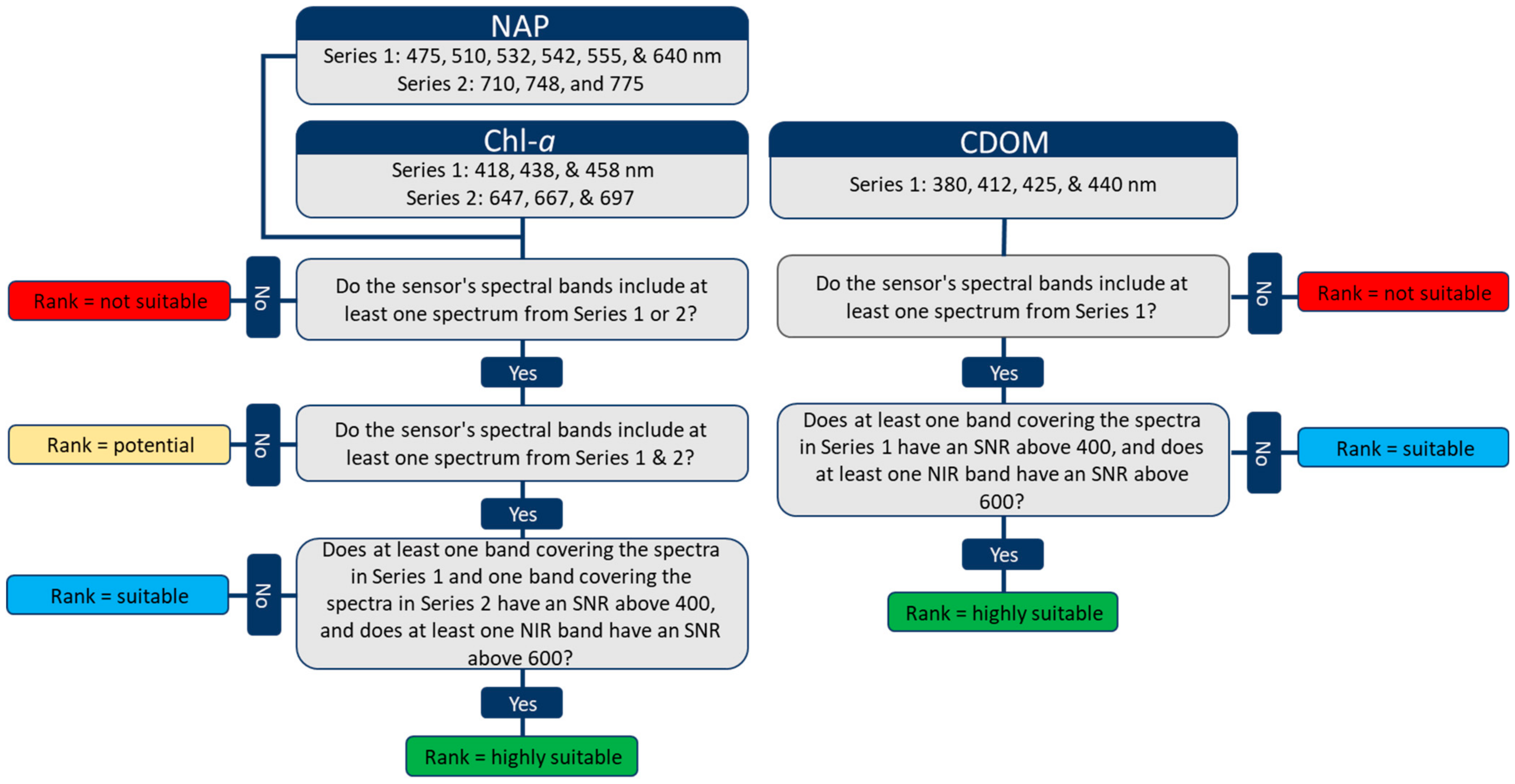
Ranking Satellite Sensors for Retrieving Chl-a, CDOM, and NAP

Table 2, adapted and updated from [18,24,57], presents a list of satellite sensors capable of retrieving WQPs, along with their specifications. Each sensor is assigned a suitability rating from “not suitable” to “highly suitable” for retrieving three optically active inland WQPs based on its spectral bands and SNR (see Figure 3). The ranking methodology is illustrated in Figure 4. As explained earlier, monitoring Chl-a and NAP concentration typically involves two series of spectral bands, while CDOM concentration typically involves one series. First, the spectral coverage of the sensor is checked to ensure it includes the useful bands. Next, the suitability of the spectral bands is assessed by verifying whether their SNR meets the minimum requirement: 400 in the visible spectrum when the NIR SNR is above 600 [53]. It is important to emphasize that the ranking assumes the selected sensor’s spatial and temporal resolutions are adequate for the intended use case. To categorize satellite sensors, a prioritization hierarchy is applied to address overlapping classifications. Sensors classified as ocean color are prioritized under the ocean color category, followed by hyperspectral sensors, and then sensors with mid-to-high spatial resolution. The remaining sensors are all geostationary.

Table 2. Overview of satellite sensors for modeling WQPs in inland waters. Green dot = highly suitable; blue dot = suitable; yellow dot = potential; red dot = not suitable; Free? = available for research. ✗ denotes sensors without SWIR band, while ✓ indicates those with SWIR band.

Type	Satellite/Sensor	Spatial Res. (m)	Spectral Res. between ~400–900 (nm) (Number of Bands)	SWIR Band	Temporal Res. (Days)	Data Record Period (Year)	Data Cost	WQPs
Type	Satellite/Sensor	Spatial Res. (m)	Spectral Res. between ~400–900 (nm) (Number of Bands)	SWIR Band	Temporal Res. (Days)	Data Record Period (Year)	Data Cost	CDOM	Chl-a	NAP
Ocean-Color	OrbView-2/SeaWiFS	1100	402–885 (8)	✗	1–2	1997–2010	Free
	OCEANSAT 1/OCM 1	360	402–885 (8)	✗	2	1999–2010	Free
	Terra, Aqua/MODIS	250, 500, 1k	405–877 (13)	✓	1–2	1999–now	Free
	Envisat/MERIS	300	407–905 (15)	✗	2–3	2002–2012	Free
	OCEANSAT 2/OCM 2	360	404–885 (8)	✗	2	2009–2022	Free
	Suomi/VIIRS	375, 750	402–885 (9)	✓	1	2011–2018	Free
	Sentinel 3/OLCI	300	392–905 (19)	✓	2–3	2016–now	Free
	GCOM-C/SGLI	250	374–878 (8)	✓	2–4	2017–2022	Free
	JPSS 1,2/VIIRS	375, 750	402–885 (9)	✓	1	2011–2018	Free
	OCEANSAT 3/OCM 3	360, 1080	407–880 (12)	✓	2	2022–now	Free
	Pace/OCI	1200	314–895 (280)	✓	1–2	2024–now	Free
	SBG	30	400–2500 (63)	✓	16	2028	Free
	GLIMR	300	340–1040 (250)	✓	4 h	2026	Free
Hyperspectral	EO-1/Hyperion	60	349–896 (60)	✓	16	2000–2017	Free
	ISS/HICO	90	380–960 (100)	✓	~3	2009–2014	Free
	ISS/DESIS	30	400–1000 (235)	✓	3–5	2018–2023	Free?
	GaoFen-5/AHSI	30	390–900 (100)	✓	5	2018–now	Free?
	PRISMA/HYC	30	400–1010 (66)	✓	29	2019–now	Free?
	ISS/HISUI	30	400–970 (60)	✓	2–60	2019–2023	Free?
	ISS/EMIT	60	381–1001 (84)	✓	~1	2022–now	Free
	EnMAP/HIS	30	420–900 (90)	✓	4, 27	2022–now	Free?
	Wyvern/Dragonette 1	5.3	503–799 (23)	✗	~2	2023–now	Charge
	Wyvern/Dragonette 2,3	5.3	445–880 (32)	✗	~2	2023–now	Charge
Mid Spatial Resolution	Landsat 1–5/MSS	60	500–1100 (4)	✗	16	1972–2013	Free
	Landsat 4,5/TM	30	450–900 (4)	✓	16	1982–2013	Free
	SPOT 4	20	500–890 (3)	✓	26	1998–2013	Charge
	Terra/ASTER	15	520–860 (3)	✓	16	1999-now	Free
	Landsat 7/ETM+	30	450–900 (4)	✓	16	1999–2022	Free
	EO 1/ALI	30	433–890 (6)	✓	16	2000–2017	Free
	PROBA-1/CHRIS	18	405–880 (17)	✓	7	2001–2021	Free
	ResourceSat-1/LISS 3	23.5	520–860 (3)	✓	24	2003–2013	Free?
	Landsat 8,9/OLI	30	433–885 (5)	✓	16	2013–now	Free
	Sentinel-2/MSI	10, 20, 60	442–875 (9)	✓	5	2015–now	Free
High Spatial Resolution	IKONOS 2	4	450–860(4)	✗	3	1999–2015	Charge
	QuickBird 2	2.4	450–900 (4)	✗	3	2001–2015	Charge
	SPOT 5	10	500–890 (3)	✓	26	2002–2015	Charge
	ResourceSat-1/LISS 4	5.8	520–860 (3)	✗	24	2003–2013	Free?
	RapidEye	6.5	440–850 (5)	✗	1	2008–2020	Charge
	GeoEye-1	1.64	450–920 (4)	✗	4	2008–now	Charge
	WorldView 2	1.8	400–1040 (8)	✗	1	2009–now	Charge
	Pléiades/HiRI	2	450–915 (4)	✗	1	2011–now	Charge
	WorldView 3	1.24	400–1040 (8)	✓	1	2014–now	Charge
	PlanetScope	3	431–885 (8)	✗	1	2014–2023	Charge
	WorldView 4	1.24	450–920 (4)	✗	1	2016–now	Charge
	SPOT 6,7	6	455–890 (4)	✗	26	2021–now	Charge
Geostationary	MSG/SEVIRI	1000	560–880 (2)	✗	15 min	2002–now	Free
	COMS/GOCI	500	402–885 (8)	✗	1 h	2010–2021	Free
	COMS/GOCI-II	250	370–885 (12)	✗	1 h	2020–now	Free
	Himawari-8, 9/AHI	1000	430–870 (4)	✓	10 min	2014–now	Free
	GOES/ABI	1000	450–880 (3)	✓	10 min	2016–now	Free

4. Atmospheric Correction for Inland Waters

Figure 5 illustrates the pathways through which sunlight can reach a satellite sensor, highlighting the complexity of AC. AC models the absorption of gasses and water vapor, Rayleigh scattering, aerosol absorption and scattering, and surface reflection at the air–water interface distorting the radiation reflected from the Earth’s surface detected at the TOA [17]. This process is challenging for water bodies, as water absorbs most light, contributing only about 10% of the radiance detected by sensors, while 90% originates from the atmosphere [46]. AC for inland waters is particularly challenging due to three factors [3]:

Light from surrounding land areas or floating objects can reflect into the sensor’s view, causing non-negligible water reflectance in the NIR region. This interference disrupts AC algorithms that use NIR to derive the aerosol type and optical thickness, potentially resulting in overcorrection of R_rs in visible wavelengths [3,58,59].
The atmosphere over inland waters is often heterogeneous due to atmospheric advection and pollution from terrestrial sources.
Inland waters typically exhibit high turbidity, leading to non-negligible reflectance in the NIR and even SWIR bands.

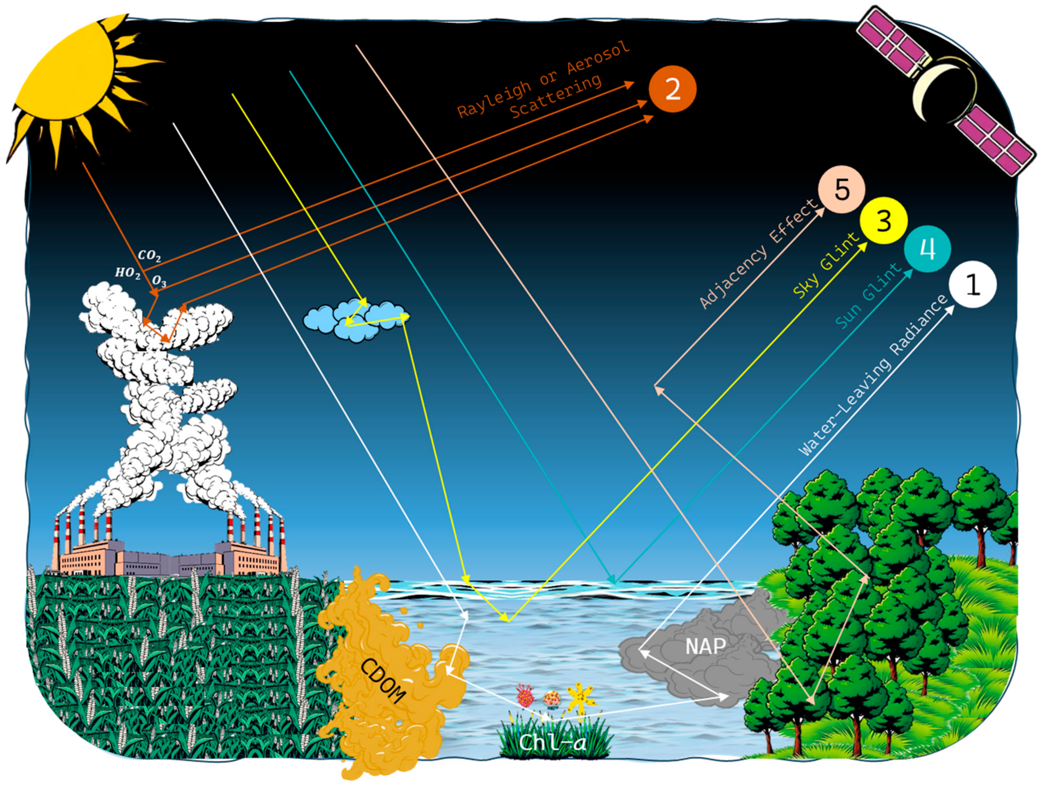
Figure 5. Concept diagram showing the pathways through which sunlight reaches a remote sensing detector. The image was generated with the help of DeepAI [60].

4.1. Additive and Multiplicative Atmospheric Effects

Atmospheric effects vary by wavelength and include additive components, such as haze, and multiplicative components, such as atmospheric transmittance [61,62]. To address additive components, simple image-based methods like Dark Object Subtraction (DOS) [63] are commonly used. DOS identifies dark objects (e.g., deep clear water or shadows) manually or through a histogram method. In the histogram approach, a sharp increase in the number of pixels at a nonzero radiance value is used to detect the dark object. The dark object radiance values are then subtracted from each pixel in the image, reducing the influence of atmospheric effects without requiring auxiliary data. Image-based methods are thus simple to implement, but their performance is often limited in inland waters [64] potentially due to atmospheric heterogeneity. To handle multiplicative effects such as downward atmospheric transmittance, the cosine of the sun zenith angle (COST) [61] method can be used. A more advanced image-based approach is the QUick AC (QUAC) algorithm [65,66], which relies on assumptions such as the presence of at least 10 endmembers and sufficiently dark pixels for baseline correction. However, these assumptions may not always hold in practice. While image-based methods have been used in various studies [67,68,69], AC algorithms based on radiative transfer models are generally preferred when meteorological data are available [70]. Examples of such models include the Second Simulation of a Satellite Signal in the Solar Spectrum (6S) [71] and libRadtran [72].

4.2. Sun Glint and Air–Water Interface Correction

AC algorithms like Fast Line-of-sight Atmospheric Analysis of Spectral Hypercubes (FLAASH), ATCOR [73], Land Surface Reflectance Code (LaSRC) [74], and Sentinel-2 Correction (Sen2Cor) [75] were designed to correct both additive and multiplicative atmospheric effects over land and water. However, they perform poorly in the removal of surface reflection at the air–water interface (e.g., sky glint and sun glint, see path #3 and #4 in Figure 5, respectively) [76], making them ineffective for inland waters.

To mitigate sun glint effects, statistical models of the sea surface, such as the Cox and Munk model [77], calculate the probability of glint based on wind speed and direction. This probability is then used to predict glint for a given wind vector, sun, and sensor position. Such methods rely on predicting glint using a probability distribution of sea surface slopes, which is effective at the 100–1000 m scale of ocean color sensors [14]. However, for higher resolution images (1–10 m), suitable for some inland waters, the pixel size may be comparable to the sea surface slopes, making statistical models of the sea surface less accurate [14]. For high-spatial-resolution images, some glint correction methods assume negligible water-leaving radiance in the NIR [78,79,80] or SWIR [81] bands or relate glint to the depth of the oxygen absorption feature [82]. Alternatively, in situations where high spatial resolution is not required, spatial aggregation could be used to facilitate statistical glint correction models to be applied to the data.

4.3. Water Vapor Absorption, Rayleigh Scattering, and Gas Absorption

Beyond sun glint, other atmospheric effects, such as water vapor absorption, Rayleigh scattering, and gas absorption could impact the accuracy of AC (see path #2 in Figure 5). Water vapor absorption can be modeled using specific absorption bands, depending on the available sensor bands [83,84]. Rayleigh scattering and gas absorption, which are generally stable [85], can be addressed with radiative transfer models like Successive Order of Scattering (SOS) [86] or 6S [87].

4.4. Aerosol Contributions

Accurately quantifying spatial and temporal variability of aerosol contributions to TOA radiance (see path #2 in Figure 5) is crucial for reliable AC [83]. One common method for estimating aerosol contributions is the black-pixel assumption in the NIR region because the water-leaving radiance (see path #1 in Figure 5) is negligible in the NIR. The NIR black-pixel method estimates aerosol type and optical thickness by analyzing the reflectance ratio in two NIR bands at the TOA, which is then extended to the visible spectrum. Over open oceans, where aerosols are largely non-absorptive and water absorption in NIR is high, this method can reach an accuracy of up to 95% [88]. However, its effectiveness is reduced for inland waters, where turbidity makes water-leaving radiance in the NIR region non-negligible [89], leading to potential overestimation of aerosol effects. Thus, three alternatives are commonly employed:

Using the SWIR black-pixel assumption for wavelengths like 1240, 1640, and 2130 nm to retrieve aerosol contributions [90]. The AC for the Operational Land Imager lite (ACOLITE) exponential extrapolation mode [50] employs this approach. However, SWIR bands often have a low SNR, especially in sensors designed for land observation like the Operational Land Imager (OLI); this can be improved by a spatially averaged filter [91] or by using a cross-calibration method from less turbid waters [92]. Additionally, not all sensors have a SWIR band. For example, as shown in Table 2, 20 out of 50 sensors lack a SWIR band, which limits the use of this approach.
Modeling marine contributions to NIR bands, a method critical for sensors like the Sea-viewing Wide Field-of-view Sensor (SeaWiFS), Medium Resolution Imaging Spectrometer (MERIS), and Geostationary Ocean Color Imager (GOCI), which lack SWIR bands. Marine contributions to NIR can be modeled by identifying the aerosol type over clear waters and transferring it to turbid waters using the nearest neighbor approach [58]. Another method involves using a bio-optical model to estimate the backscattering of particles in the NIR band from the backscattering of particles in the green band (e.g., 670 nm) and subsequently calculating the water-leaving radiance in the NIR, after which the NIR black-pixel assumption AC algorithm is applied [93]. Alternatively, aerosol scattering in NIR bands can be calculated by assuming spatial homogeneity in the NIR band ratios for aerosol and water-leaving reflectance [59].
Combining or switching between NIR and SWIR bands is a method where turbid pixels are processed using the SWIR-based AC algorithms, while non-turbid pixels are handled with the NIR-based AC algorithms. This method has been applied in the SeaDAS [94] and the Level 2 generator (L2gen) [90]. However, the success of L2gen depends on accurately determining the aerosol type.

Besides NIR/SWIR black-pixel assumption methods, other methods have been developed for AC over inland waters. For instance, the ACOLITE’s Dark Spectrum Fitting (DSF) mode [87,95], an image-based method, estimates the aerosol type and optical thickness by selecting black targets with the lowest observed TOA reflectance across all available bands. This approach differs from traditional methods that rely on predefined dark bands, such as NIR and SWIR. Thus, it minimizes the risk of overcorrected reflectance after the AC process.

Land-based methods, such as Image correction for atmospheric effects (iCOR) [96] and the AC algorithm for inLand and Nearshore Coastal waters (ACLANC) [97], extend aerosol information from dark land pixels (like dark vegetation) or adjacent areas to water areas. These methods, however, perform poorly due to the limited availability or absence of dark land pixels and the variable aerosol properties across different terrains due to terrestrial sources.

Neural Network (NN)-based AC algorithms simultaneously retrieve R_rs and optically active WQPs by analyzing the visible and NIR TOA radiance. The Ocean Color Simultaneous Marine and Aerosol Retrieval Tool (OC-SMART) [98], Case 2 Regional Coast Color (C2RCC) [99], Case2eXtreme (C2X) [100], and C2X Complex Net (C2XC) are examples of NN-based AC algorithms. A recent study has shown that the use of NN-based AC algorithms for Multispectral Imagers (MSIs) is increasing [101], likely due to their assumption-free nature, ease of implementation, or applicability across a range of water conditions, from very clear to ultra-oligotrophic [102]. NN-based AC algorithms perform according to the dataset they are trained on, and they therefore tend to produce better results when the IOP values in the areas where they are applied match those in the training dataset. For example, a study comparing C2RCC, C2X, and C2XC to retrieve Chl-a using MSIs in 32 small reservoirs across Spain found that C2RCC outperformed the other models [103], likely due to differences in training datasets. Because NN-based AC algorithms’ performance depends on the training data, their usefulness can be limited in heterogeneous inland waters. The NN-based AC algorithms mentioned above depend on several auxiliary data —such as salinity, temperature, ozone concentration, atmospheric pressure, and elevation—limiting their use as these auxiliary data are not always readily available. Spectral-based algorithms employ either spectral optimization, such as POLYMER [86], or spectral fitting, such as Glint Removal for Sentinel-2 (GRS) [81], to simultaneously correct for aerosol and sun glint contributions. These algorithms require substantial computational resources. Alternatively, the Empirical Line Method (ELM) [104] uses in situ reflectance spectra and applies linear regression for each band to adjust the surface reflectance. While effective, ELM requires concurrent in situ spectra, which are not always available.

4.5. Adjacency Effect

The AE, which occurs when light from surrounding land areas reflects into the sensor view (see #5 in Figure 5), complicates AC, especially over inland waters [3]. This effect, influenced by aerosol optical thickness, scene geometry, and topography, can be observed on water pixels up to 36 km from the coast [105]. To resolve this issue, the Improving Contrast between Ocean and Land (ICOL) processor, designed for the MERIS sensor, applies AE correction to the TOA signal before the AC process. However, it remains unadopted for mid-to-high spatial resolution sensors like OLI or MSI, widely used in inland water studies. The SIMilarity Environment Correction (SIMEC) method [106], used in Sen2Cor and iCOR, assumes that water’s spectral shape in the NIR range is stable. However, it relies on assumptions related to red-edge and NIR bands, making it sensitive to factors such as shallow water, turbidity, and algal blooms. The SIMEC method may perform poorly due to its insufficient consideration of the aerosol type and concentration, the complexity of three-dimensional (3D) geometry, and the variability in spectral reflectance across different land cover types. Simple AE correction is supported by 6S, but it is limited to isotropically reflecting objects, making it less suitable for inland water studies.

Correcting for the AE requires defining the point spread function of the atmosphere, which explains the origin of scattered radiation from the Earth’s surface and how radiation from different surface areas contributes to the measurements made by the sensor [107]. Some methods have been developed to address the point spread function, such as [108], which calculates azimuthally symmetric point spread functions for Lambertian surfaces. However, this method performs poorly with off-nadir observations and water specular reflectance. Additionally, the Adaptive Window by Proportion (AWP-Inland Water) model uses the point spread function to compute the contribution of the AE for the MSI [109]. The AWP-Inland Water model estimates the horizontal range of the AE required to compute reflectance due to the AE on a pixel-by-pixel basis, considering the proportion of land and water pixels within a 5 km window. A recent study introduced the Remote Sensing Adjacency Correction (RAdCor) method [110], a physics-based approach for correcting adjacency effects. RAdCor constructs the point spread function by simulating the top-of-atmosphere radiance generated by a single unit-reflectance pixel surrounded by non-reflective neighbors. Using the 6SV radiative transfer model, RAdCor estimates how radiance from surrounding land pixels is scattered into the sensor’s view. By repeating this simulation across different distances and directions, RAdCor derives a scene-specific 2D point spread function, enabling correction over heterogeneous inland water environments. Recent studies have employed 3D Monte Carlo methods [107,111,112] to account for the AE by incorporating diverse atmospheric profiles and topographies, simulating light transfer in a 3D ocean–land–atmosphere system. Additionally, the Genetic Algorithm for AC (GAAC) method [113] retrieves the AE by solving a set of physics-based equations with seven unknown variables, including the aerosol optical depth and type, using a genetic algorithm. The number of equations matches the number of sensor spectral bands, excluding SWIR bands.

4.6. Comparison of Atmospheric Correction Algorithms for OLI and MSI Sensors

Recent studies have compared AC algorithms across different sensors to evaluate their effectiveness in retrieving R_rs and WQPs. The OLI onboard Landsat 8 and 9 and the MSI onboard Sentinel-2 have been frequently used in inland water studies. As shown in Figure 1, the number of publications related to these sensors has notably increased since their launch. The following highlights recent studies comparing AC algorithms in this context. For the OLI sensor, two image-based AC algorithms (DOC and COST), three physics-based algorithms (ACOLITE’s exponential extrapolation mode, ATCOR, and FLAASH), and TOA reflectance were compared to estimate suspended particulate matter [62]. The image-based methods outperformed TOA reflectance and physics-based methods, with the latter underperforming due to poor atmospheric inputs and overcorrection. In another study with OLI data, ACOLITE’s DSF mode, C2RCC, iCOR, L2gen, and POLYMER were evaluated for retrieving R_rs by comparing them with a global set of in situ R_rs measurements [114], finding that L2gen was the most accurate method.

For the MSI sensor, AC algorithms used for monitoring Chl-a concentration have been summarized [100], highlighting the frequent application of Sen2Cor, ACOLITE’s DSF mode, C2RCC, and POLYMER. However, TOA reflectance has remained frequently used in most ecosystems except marine environments [100]. POLYMER and C2RCC have been found to provide the best statistical outcomes when compared with ACOLITE’s DSF mode, iCOR, L2gen, and Sen2Cor for retrieving R_rs [115,116]. Additionally, ACOLITE’s DSF mode, C2RCC, FLAASH, iCOR, and L2gen have been evaluated by comparing observed and estimated R_rs [89]; iCOR performed best in the Blue and NIR bands, while ACOLITE’s DSF mode performed best in the green and red bands.

In one study, algorithms such as L2gen, ACOLITE’s DSF mode, Sen2Cor, LaSRC, iCOR, C2RCC, C2X, and POLYMER were compared for R_rs retrieval from for both OLI and MSI [117]. The results showed that ACOLITE’s DSF mode preserved the spectral shape the best, while NN-based AC algorithms had the lowest errors and bias. Another similar study [118] evaluated ACOLITE’s DSF mode, OC-SMART, SeaDAS, C2X, POLYMER, and iCOR, identifying iCOR, OC-SMART, and ACOLITE’s DSF mode as top performers.

In conclusion, various AC algorithms have been developed, each with unique strengths and limitations, as summarized in Table 3. No single approach consistently performs the best across all inland waters and sensors. Consequently, in some cases, researchers use raw TOA data without AC for modeling WQPs via empirical models, such as cyanobacteria [119,120] and Chl-a [100]. Furthermore, while various AE algorithms have been introduced recently, their performance in retrieving WQPs remains largely unassessed and warrants further investigation.

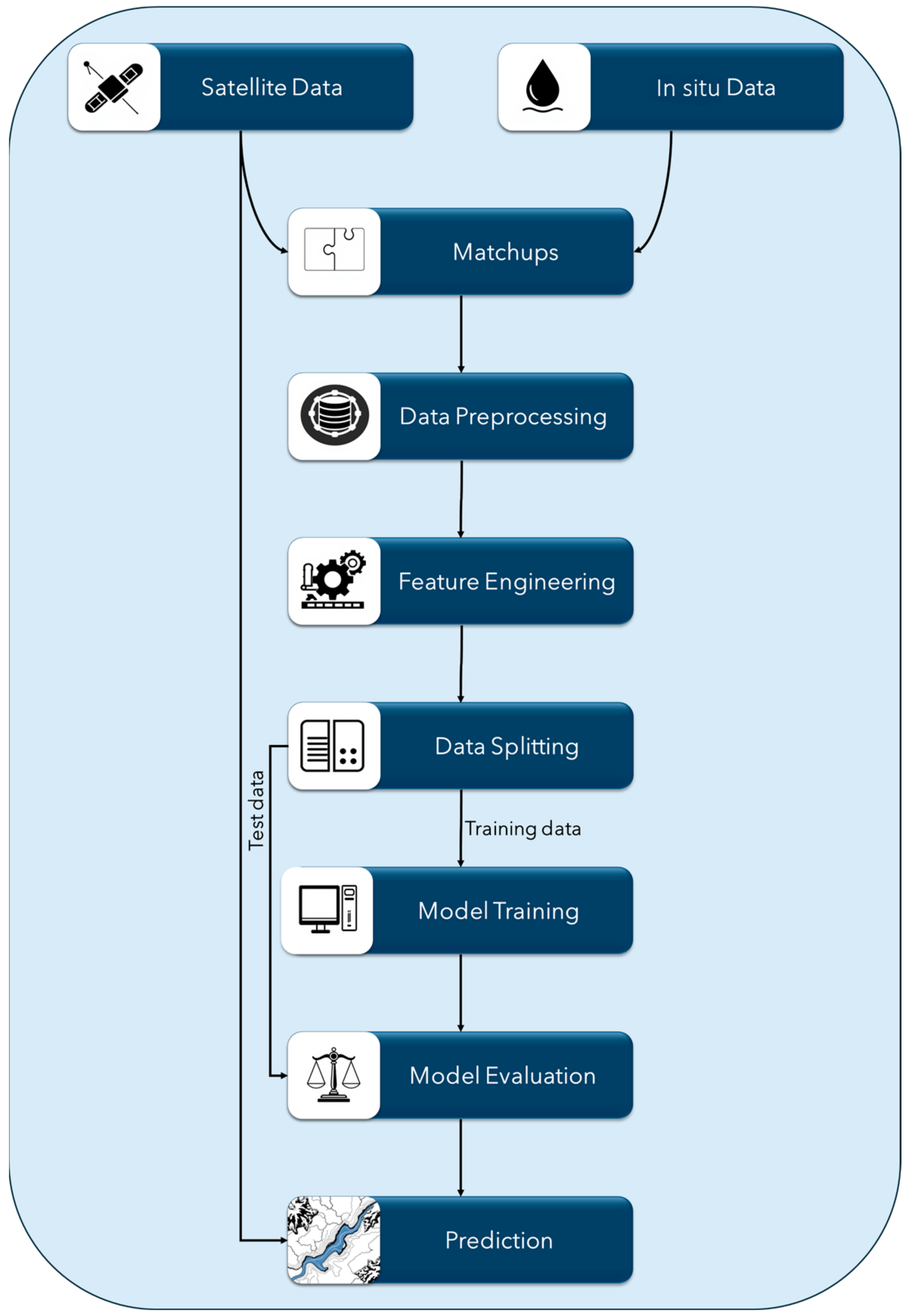
5. Machine Learning Models for Retrieving Water Quality Parameters

ML models are algorithms that make predictions of a variable (the response) based on data related to that variable (the predictors); these models are trained to recognize relationships between the predictors and the response through optimizing model parameters to minimize a cost function, e.g., the difference between the predictions and a set of validation data. One of the primary types of ML models is the supervised model, where labeled data are used to train the model. In supervised machine learning, as illustrated in Figure 6, the process begins with satellite and in situ data. These are then combined through a matchup process to align the corresponding observations. Next, optional data preprocessing steps may be performed to clean the data, remove outliers, normalize and transform variables, and handle missing values. This is followed by feature engineering, where meaningful features, such as value from spectral bands or indices, are derived from the raw data. The dataset is then split into training and test sets, with the training data used for model training to learn patterns. The trained model is then assessed through model evaluation using the test data to measure its performance. Finally, the model is applied for prediction. Supervised models can be divided into four major categories:

Statistical models, which include linear models like ordinary least squares regression and non-linear models like generalized additive models;
Kernel-based models, such as support vector regression, which operate by mapping input variables into higher-dimensional feature spaces using a kernel function;
Tree-based models, such as Decision Trees (DTs), which are structured hierarchically, with each node representing a decision based on a specific feature;
NN models, such as multilayer perceptrons, which process raw data through multiple layers, each transforming the data into more abstract representations than the previous layer.

Numerous studies have compared ML model performance for retrieving inland WQPs [32,37,119,121,122,123,124,125,126,127,128,129,130,131,132,133,134,135,136,137]. Recent review studies have examined ML models used for estimating organic matter and harmful algal blooms [138], TDS and TSS [38], and Chl-a [101]. These reviews generally conclude that no single ML model consistently outperforms others across all WQPs and study areas [139]. However, a key takeaway is that empirical methods, particularly ML models, generally outperform other bio-optical models in estimating WQPs [15,101,139]. It should be noted, however, that the performance of empirical methods is often limited to the specific regions or conditions on which they were trained, as discussed in Section 5.1. In contrast, other bio-optical models may offer better performance for extrapolation. This review focuses on the challenges associated with ML models and recent efforts to overcome them.

5.1. Improving Accuracy and Generalization in Machine Learning

One approach for improving ML model performance in modeling WQPs is ensemble modeling, where the outputs of several ML models are combined. For example, multiple DTs can form an ensemble model like random forest [140] or extreme gradient boosting [141,142]. The underlying assumption is that an ensemble model can yield more reliable predictions in regression tasks and enhance the model’s generalization by capturing diverse relationships that might be missed when relying on a single regression method. It is also possible to combine the outputs of different ML methods using simple mathematical operators, such as averaging [143], or statistical methods like least absolute shrinkage and selection operator [144] and BayesianRidge [145]. Another method for combining ML outputs is Bayesian maximum entropy-based fusion [121,128], which integrates the predictions of different ML models using weighted averaging.

The main advantage of ML is its lack of assumptions (e.g., about atmospheric composition). However, due to the absence of a physical basis, ML models often perform poorly when applied beyond their calibrated range, resulting in unreliable predictions during extrapolation in ML models. To address this, a global model was developed using a Mixture Density Network (MDN) trained on optically active WQPs from various locations worldwide [146,147]. However, the MDN has certain shortcoming: (1) it is sensitive to uncertainties in the AC process, which can affect its performance under different atmospheric or water conditions [147,148,149], and (2) it may not perform well when the target WQPs fall outside its calibrated range. For example, the globally trained MDN overestimated C-Phycocyanin concentration in the Billings Reservoir [120], likely due to a lower C-Phycocyanin to Chl-a ratio compared to the global training dataset used for MDN calibration [150]. Similarly, another study [151] trained a random forest model using both local and global datasets (i.e., GLORIA dataset [152]) to map Secchi disk depth in the Finger Lakes, USA. The results showed that the locally trained model outperformed the global one, possibly because the GLORIA dataset is skewed toward eutrophic water bodies, and as a result, the global model may be biased when applied to oligotrophic waters like the Finger Lakes. Therefore, it appears that locally trained ML models generally outperform globally trained ones when evaluated within the same region that the locally trained ML models were trained on. However, this performance advantage may not hold when applied to new or unseen locations.

5.2. Challenges and Solutions for Addressing Spatial and Temporal Autocorrelation in Machine Learning Models

Spatial and temporal autocorrelation occurs when nearby data points influence each other or are impacted by the same spatially/temporally variable factors. This is generally present in spatial data, such as satellite imagery. Autocorrelation indicates that unmodeled spatial/temporal processes might be influencing the variable of interest [153] and violates the independence assumption, leading to biased estimates and unreliable conclusions. Moreover, based on Tobler’s First Law of Geography [154], assessing spatial autocorrelation in model residuals is crucial for spatial regression models [37,155] because identification of spatial patterns in residuals helps determine whether the model captures all spatial dependencies in the data.

Importantly, for estimating spatial/temporal parameters like WQPs, data-driven methods need to be evaluated to understand the extent to which their outputs are influenced by spatial autocorrelation [29]. This is crucial because these methods rely solely on data, without a physical foundation built in to the model structure [28]. Moran’s I is the most commonly used statistical tool to evaluate spatial autocorrelation [144,153,156,157]. To address spatial autocorrelation, several methods have been proposed. The spatial lag and spatial error models [158] account for autocorrelation by incorporating spatially lagged variables or spatially correlated error terms. Additionally, the geographically weighted regression model [159] enables localized modeling by incorporating spatially varying coefficients based on geographical coordinates. Another strategy is to include spatial and temporal information as input features. Although this may reduce the model’s capacity for extrapolation, it enhances the ability to capture spatial and temporal patterns, leading to improved model performance for the training area. This was demonstrated in multiple studies [39,130,131,160] where longitude, latitude, month, day of the week, and day of the year were used as spatial and temporal parameters.

A related issue is information leakage between training and test sets. This occurs when spatial autocorrelation exists between the training set samples and the surrounding test set samples [161]. For example, if test and training data are split randomly, adjacent spatially autocorrelated data points will often end up in both sets, leading to overestimation of model performance caused by incomplete independence between the datasets [28]. Other methods for splitting training and test datasets, such as leave-one-out [146], K-fold cross-validation [145,162,163], or Monte Carlo simulations [120], have been employed in previous studies. However, like random splitting, they do not ensure the complete prevention of information leakage. Methods like spatial or temporal cross-validation [130], checkerboard evaluation [164], and block or buffered cross-validation [165] have been employed in previous studies to reduce or prevent information leakage. These methods train models on data from certain regions or periods and evaluate their performance on data from different regions or periods [166].

5.3. Enhancing Dimensionality in Inland Water Remote Sensing

Since ML models are data-driven, their accuracy largely depends on the quality, quantity, and dimensionality of training data. Generally, more training data lead to better model performance. Moreover, the quality, quantity, and dimensionality of the training dataset exert a higher influence on model performance than the data-driven modeling approach itself [28]. The quality of data can be improved during the “data preprocessing” step (see Figure 6). This step involves cleaning the data, removing outliers, normalizing and transforming variables, and handling missing values to enhance overall data quality. To increase the quantity of training data, one possible approach is the use of generative artificial intelligence to create synthetic data. For instance, a recent study [167] employed a Generative Adversarial Network (GAN) for data augmentation, generating synthetic training data to enhance water quality management via RS.

Unlike terrestrial RS, which utilizes high-dimensional data such as spectral bands, spatial patterns, 3D modeling, and polarization, RS of inland waters is constrained to fewer dimensions, primarily spectral bands. This limitation reduces the ability to develop the multiple layers of representation needed to train complex ML models effectively. To overcome this limitation and enhance data dimensionality, recent studies have incorporated auxiliary data and spectral indices in inland and coastal water studies. For instance, some studies have utilized water salinity, water currents, and bathymetry data [131] or water temperature and wind speed [142] to map eutrophication indicators. For example, a study on Lake Simcoe in Toronto, Canada [168], employed a wide range of auxiliary data, including air temperature, sea level, precipitation, wind speed and direction, water temperature, urban and farmland areas, nighttime light (as an indicator of economic development and human activity), and the number of mobile devices connected to cellular towers (as a proxy for population distribution) to map Chl-a, total phosphorus, total nitrogen, Secchi disk depth, dissolved organic carbon, and dissolved oxygen. In this context, the degree of polarization provided by the OCI could be considered a new dimension for enhancing future studies, adding another layer of information that could improve the accuracy of inland WQP estimation.

Another approach is to extract more information from spectral bands through feature engineering. For example, spectral indices combine different spectral bands through mathematical operations, either linearly or nonlinearly, and have been used in recent studies to improve the performance of ML models [124,140,169,170]. Furthermore, derivative spectroscopy has emerged as a novel method for extracting spectral features in inland water studies using hyperspectral data. Derivative spectroscopy leverages integer-order [171] or fractional-order derivatives [32,140], enabling the representation of higher-order derivatives.

6. Conclusions

This study reviewed decommissioned, active, and future sensors that have the potential to estimate WQPs in inland waters. We also discussed proposed AC algorithms and the challenges of estimating WQPs using ML approaches, along with proposed solutions. Below, we summarize key findings and offer recommendations for future research on WQP modeling in inland waters:

Not all sensors are suitable for retrieving Chl-a, CDOM, and NAP concentrations. Before initiating modeling, it is important to address whether the selected sensor can effectively model the target WQP (Table 2). Leveraging a multi-sensor integration strategy - especially combining sensors with complementary strengths - can help overcome individual limitations.
High spatial resolution sensors may lack the necessary spectral resolution and SNR for inland WQP estimation, but they are the only option for small inland waters.
The Surface Biology and Geology (SBG) sensor, set to launch in 2028, is highly suitable for modeling Chl-a, NAP, and CDOM concentrations (Table 2). It has spatial and temporal resolutions similar to the Landsat OLI but offers higher spectral resolution, an improved SNR, and a tilting mechanism to minimize sun glint, making it highly suitable for inland WQP monitoring. However, its performance remains to be validated once operational data become available.
No AC algorithm has consistently outperformed others across all atmospheric and water conditions. Therefore, it is important to evaluate the suitability of a given algorithm for the specific sensor, water type, and atmospheric context before implementation. Moreover, although new AE correction methods have been proposed in recent research, their performance has not been thoroughly evaluated.
Recent studies demonstrate that ensemble methods achieve higher accuracy and robustness compared to single machine learning models.
Locally trained ML models generally outperform globally trained ones when evaluated within the same region the local model was trained on. This is because ML models tend to perform poorly in regions where they have not been calibrated, due to differences in atmospheric conditions or variations in WQP concentrations between the training data and the target area.
Addressing the impact of spatial and temporal autocorrelation in WQP modeling is important, particularly when using data-driven models, as it can result in biased estimates and unreliable conclusions. Additionally, identifying spatial patterns in residuals is key to assessing whether the model has captured all spatial dependencies in the data.
Ensuring the prevention of information leakage during the separation of training and test data is necessary for reliable performance evaluation. Such leakage can lead to inflated performance estimates and undermine the validity of the results. Methods like spatial/temporal cross-validation, checkerboard evaluation, and buffered cross-validation help mitigate the risk of information leakage.
Increasing data dimensionality through the integration of auxiliary variables—such as meteorological parameters—can improve the performance of ML models. This approach compensates for the limited spectral and spatial information typically available in inland water RS and allows models to capture more complex patterns. However, this may lead to overfitting if cross-validation and regularization techniques are not properly applied.

Improvements in WQP monitoring over the coming years are likely to result from gradual improvements in sensor characteristics, data quality, AC, and other pre-processing factors, as well as improvements in ML models and an understanding of how to apply such models effectively to the available data. Improvements may come from these components in isolation; for example, improved ML models, e.g., from deep learning, may produce better WQP monitoring on their own, independently of other factors. Or improvement may come from combinations of factors, such as ML models being increasingly able to extract information from the additional dimensionality of hyperspectral data or the varied information provided through multi-sensor integration. In this study, we have identified some of the most promising avenues for future improvement in WQP monitoring using remote sensing technology, and real-world testing will demonstrate which of these will provide the greatest value over the coming years.

Author Contributions

M.A. (Mohsen Ansari): conceptualization, data curation, formal analysis, investigation, methodology, resources, visualization, writing—original draft. A.K.: conceptualization, methodology, project administration, supervision, writing—review and editing. M.A. (Meisam Amani): writing—review and editing. M.S.: writing—review and editing. All authors have read and agreed to the published version of the manuscript.

Funding

This research received no external funding.

Data Availability Statement

No new data were created or analyzed in this study.

Acknowledgments

Declaration of generative AI and AI-assisted technologies in the writing process: During the preparation of this work, we used OpenAI’s ChatGPT (GPT-4-turbo) for English grammar corrections. For Figure 5 and Figure 6, image generation was assisted by DeepAI. After using these tools, we thoroughly reviewed and edited the content as needed and take full responsibility for the content of the publication.

Conflicts of Interest

The authors declare no conflict of interest.

Abbreviations

The following abbreviations are used in this manuscript:

SeaWiFS	Sea-viewing Wide Field-of-view Sensor
OCM	Ocean Color Monitor
JPSS	Joint Polar Satellite System
VIIRS	Visible Infrared Imaging Radiometer Suite
OLCI	Ocean and Land Color Instrument
SGLI	Second Generation Global Imager
OCI	Ocean Color Imager
GLIMR	Geostationary Littoral Imaging and Monitoring Radiometer
HICO	Hyperspectral Imager for the Coastal Ocean
AHI	Advanced Himawari Imager
AHSI	Advanced Hyperspectral Imager
HYC	Hyperspectral Camera
COMS	Communication, Ocean, and Meteorological Satellite
EMIT	Earth Surface Mineral Dust Source Investigation
MSS	Multispectral Scanner
TM	Thematic Mapper
ASTER	Advanced Spaceborne Thermal Emission and Reflection Radiometer
ETM+	Enhanced Thematic Mapper Plus
ALI	Advanced Land Imager
CHRIS	Compact High Resolution Imaging Spectrometer
MODIS	Moderate Resolution Imaging Spectroradiometer
SPOT	Satellite Pour l’Observation de la Terre
MSI	Multispectral Imager
HiRI	High Resolution Imager
SEVIRI	Spinning Enhanced Visible and InfraRed Imager
GOCI	Geostationary Ocean Color Imager
OLI	Operational Land Imager
ABI	Advanced Baseline Imager
MERIS	Medium Resolution Imaging Spectrometer
PACE	Plankton, Aerosol, Cloud, ocean Ecosystem
SBG	Surface Biology and Geology
EO	Earth Observing
ISS	International Space Station
EnMAP	Environmental Mapping and Analysis Program
LISS	Linear Imaging and Self-Scanning Sensor
MSG	Meteosat Second Generation
HISUI	Hyperspectral Imager Suite
GOES	Geostationary Operational Environmental Satellite
PROBA	Project for On-Board Autonomy
HIS	Hyperspectral Imager
DESIS	DLR Earth Sensing Imaging Spectrometer

Appendix A

We defined the search terms to minimize temporal bias and ensure broad coverage of relevant studies. Nonetheless, we acknowledge that shifts in terminology, such as the transition from “machine learning” to “AI”, may influence search trends.

The following query formulations were used to retrieve publications for trend analysis in Figure 1:

Query 1: (“inland water*” OR “river*” OR “lake*” OR “reservoir*” OR “wetland*” OR “freshwater” OR “estuary*” OR “aquatic system*”) AND (“remote sensing” OR “satellite imagery” OR “Earth observation” OR “hyperspectral imaging” OR “multispectral imaging”) AND (“water quality” OR “turbidity” OR “chlorophyll*” OR “total suspended solid*” OR “total dissolved solid*” OR “salinity” OR “colored dissolved organic matter” OR “dissolved organic carbon” OR “particulate organic carbon” OR “electrical conductivity” OR “Secchi disk depth” OR “eutrophication” OR “harmful algal bloom*” OR “phytoplankton” OR “cyanobacteria” OR “non-algal particle*” OR “water transparency” OR “biogeochemical cycle*” OR “optically active constituent*” OR “optically inactive constituent*” OR “non-optically active constituent*”);
Query 2: (“empirical model*” OR “data-driven model*” OR “statistical model*” OR “supervised learning” OR “unsupervised learning” OR “regression” OR “machine learning” OR “deep learning” OR “statistical analysis” OR “linear regression” OR “Bayesian” OR “ensemble learning “);
Query 3: (“machine learning” OR “deep learning” OR “Bayesian” OR “ensemble learning “);
Query 4: (“physical model*” OR “mechanistic model*” OR “analytical model*” OR “semi-analytical model*” OR “quasi-analytical model*” OR “radiative transfer model*” OR “radiative transfer code*” OR “radiative transfer equation*”).

References

Likens, G.E. Inland Waters. In Encyclopedia of Inland Waters; Academic Press: Oxford, UK, 2009; pp. 1–5. ISBN 978-0-12-370626-3. [Google Scholar]
Bastviken, D.; Tranvik, L.J.; Downing, J.A.; Crill, P.M.; Enrich-Prast, A. Freshwater Methane Emissions Offset the Continental Carbon Sink. Science 2011, 331, 50. [Google Scholar] [CrossRef] [PubMed]
Mishra, D.R.; Ogashawara, I.; Gitelson, A.A. Bio-Optical Modeling and Remote Sensing of Inland Waters; Elsevier: Amsterdam, The Netherlands, 2017; ISBN 978-0-12-804654-8. [Google Scholar]
United Nations. The United Nations World Water Development Report 2023: Partnerships and Cooperation for Water; UNESCO: Paris, France, 2023. [Google Scholar]
Franco; Granados, E.; Kuritzky, M.; Lukacs, R.; Zahidi, S. The Global Risks Report 2020; World Economic Forum: Cologny, Switzerland, 2020. [Google Scholar]
Mueller, J.T.; Gasteyer, S. The Widespread and Unjust Drinking Water and Clean Water Crisis in the United States. Nat. Commun. 2021, 12, 3544. [Google Scholar] [CrossRef] [PubMed]
Barati, A.A.; Pour, M.D.; Sardooei, M.A. Water Crisis in Iran: A System Dynamics Approach on Water, Energy, Food, Land and Climate (WEFLC) Nexus. Sci. Total Environ. 2023, 882, 163549. [Google Scholar] [CrossRef]
Getirana, A.; Libonati, R.; Cataldi, M. Brazil Is in Water Crisis—It Needs a Drought Plan. Nature 2021, 600, 218–220. [Google Scholar] [CrossRef]
Christodoulou, A.; Christidis, P.; Bisselink, B. Forecasting the Impacts of Climate Change on Inland Waterways. Transp. Res. Part Transp. Environ. 2020, 82, 102159. [Google Scholar] [CrossRef]
Yao, S.; Chen, C.; He, M.; Cui, Z.; Mo, K.; Pang, R.; Chen, Q. Land Use as an Important Indicator for Water Quality Prediction in a Region under Rapid Urbanization. Ecol. Indic. 2023, 146, 109768. [Google Scholar] [CrossRef]
Parmar, T.K.; Rawtani, D.; Agrawal, Y.K. Bioindicators: The Natural Indicator of Environmental Pollution. Front. Life Sci. 2016, 9, 110–118. [Google Scholar] [CrossRef]
Klemas, V. Remote Sensing of Algal Blooms: An Overview with Case Studies. J. Coast. Res. 2011, 28, 34–43. [Google Scholar] [CrossRef]
National Research Council. The Drama of the Commons; National Academies Press: Washington, DC, USA, 2002; ISBN 978-0-309-08250-1. [Google Scholar]
Kay, S.; Hedley, J.D.; Lavender, S. Sun Glint Correction of High and Low Spatial Resolution Images of Aquatic Scenes: A Review of Methods for Visible and Near-Infrared Wavelengths. Remote Sens. 2009, 1, 697–730. [Google Scholar] [CrossRef]
Sagan, V.; Peterson, K.T.; Maimaitijiang, M.; Sidike, P.; Sloan, J.; Greeling, B.A.; Maalouf, S.; Adams, C. Monitoring Inland Water Quality Using Remote Sensing: Potential and Limitations of Spectral Indices, Bio-Optical Simulations, Machine Learning, and Cloud Computing. Earth-Sci. Rev. 2020, 205, 103187. [Google Scholar] [CrossRef]
Declaro, A.; Kanae, S. Enhancing Surface Water Monitoring through Multi-Satellite Data-Fusion of Landsat-8/9, Sentinel-2, and Sentinel-1 SAR. Remote Sens. 2024, 16, 3329. [Google Scholar] [CrossRef]
International Ocean-Colour Coordinating Group (IOCCG). Atmospheric Correction for Remotely-Sensed Ocean-Colour Products; IOCCG Report Series; International Ocean Colour Coordinating Group: Dartmouth, NS, Canada, 2010. [Google Scholar]
International Ocean-Colour Coordinating Group (IOCCG). Earth Observations in Support of Global Water Quality Monitoring; IOCCG Report Series; International Ocean Colour Coordinating Group: Dartmouth, NS, Canada, 2018. [Google Scholar]
Smith, R.C.; Baker, K.S. The Bio-Optical State of Ocean Waters and Remote Sensing. Limnol. Oceanogr. 1978, 23, 247–259. [Google Scholar] [CrossRef]
Gholizadeh, M.H.; Melesse, A.M.; Reddi, L. A Comprehensive Review on Water Quality Parameters Estimation Using Remote Sensing Techniques. Sensors 2016, 16, 1298. [Google Scholar] [CrossRef]
Tesfaye, A. Remote Sensing-Based Water Quality Parameters Retrieval Methods: A Review. East Afr. J. Environ. Nat. Resour. 2024, 7, 80–97. [Google Scholar] [CrossRef]
Vakili, T.; Amanollahi, J. Determination of Optically Inactive Water Quality Variables Using Landsat 8 Data: A Case Study in Geshlagh Reservoir Affected by Agricultural Land Use. J. Clean. Prod. 2020, 247, 119134. [Google Scholar] [CrossRef]
Chen, L.; Liu, L.; Liu, S.; Shi, Z.; Shi, C. The Application of Remote Sensing Technology in Inland Water Quality Monitoring and Water Environment Science: Recent Progress and Perspectives. Remote Sens. 2025, 17, 667. [Google Scholar] [CrossRef]
Matthews, M.W. A Current Review of Empirical Procedures of Remote Sensing in Inland and Near-Coastal Transitional Waters. Int. J. Remote Sens. 2011, 32, 6855–6899. [Google Scholar] [CrossRef]
Deng, Y.; Zhang, Y.; Pan, D.; Yang, S.X.; Gharabaghi, B. Review of Recent Advances in Remote Sensing and Machine Learning Methods for Lake Water Quality Management. Remote Sens. 2024, 16, 4196. [Google Scholar] [CrossRef]
Elmotawakkil, A.; Enneya, N.; Bhagat, S.K.; Ouda, M.M.; Kumar, V. Advanced Machine Learning Models for Robust Prediction of Water Quality Index and Classification. J. Hydroinformatics 2025, 27, 299–319. [Google Scholar] [CrossRef]
Koldasbayeva, D.; Tregubova, P.; Gasanov, M.; Zaytsev, A.; Petrovskaia, A.; Burnaev, E. Challenges in Data-Driven Geospatial Modeling for Environmental Research and Practice. Nat. Commun. 2024, 15, 10700. [Google Scholar] [CrossRef]
Gray, P.C.; Boss, E.; Prochaska, J.X.; Kerner, H.; Demeaux, C.B.; Lehahn, Y. The Promise and Pitfalls of Machine Learning in Ocean Remote Sensing. Oceanography 2024, 37, 52–63. [Google Scholar] [CrossRef]
Liu, X.; Kounadi, O.; Zurita-Milla, R. Incorporating Spatial Autocorrelation in Machine Learning Models Using Spatial Lag and Eigenvector Spatial Filtering Features. ISPRS Int. J. Geo-Inf. 2022, 11, 242. [Google Scholar] [CrossRef]
Cao, Z.; Ma, R.; Duan, H.; Xue, K. Effects of Broad Bandwidth on the Remote Sensing of Inland Waters: Implications for High Spatial Resolution Satellite Data Applications. ISPRS J. Photogramm. Remote Sens. 2019, 153, 110–122. [Google Scholar] [CrossRef]
Dekker, A.G.; Pinnel, N.; Gege, P.; Briottet, X.; Court, A.; Peters, S.; Turpie, K.R.; Sterckx, S.; Costa, M.; Giardino, C.; et al. Feasibility Study for an Aquatic Ecosystem Earth Observing System Version 1.2. In Feasibility Study for an Aquatic Ecosystem Earth Observing System; CEOS: Rapid City, SD, USA, 2018. [Google Scholar]
Fu, B.; Li, S.; Lao, Z.; Wei, Y.; Song, K.; Deng, T.; Wang, Y. A Novel Hierarchical Approach to Insight to Spectral Characteristics in Surface Water of Karst Wetlands and Estimate Its Non-Optically Active Parameters Using Field Hyperspectral Data. Water Res. 2024, 257, 121673. [Google Scholar] [CrossRef]
Zhou, Y.; Li, W.; Cao, X.; He, B.; Feng, Q.; Yang, F.; Liu, H.; Kutser, T.; Xu, M.; Xiao, F.; et al. Spatial-Temporal Distribution of Labeled Set Bias Remote Sensing Estimation: An Implication for Supervised Machine Learning in Water Quality Monitoring. Int. J. Appl. Earth Obs. Geoinf. 2024, 131, 103959. [Google Scholar] [CrossRef]
D’Sa, E.J.; Hu, C.; Muller-Karger, F.E.; Carder, K.L. Estimation of Colored Dissolved Organic Matter and Salinity Fields in Case 2 Waters Using SeaWiFS: Examples from Florida Bay and Florida Shelf. J. Earth Syst. Sci. 2002, 111, 197–207. [Google Scholar] [CrossRef]
Siddorn, J.R.; Bowers, D.G.; Hoguane, A.M. Detecting the Zambezi River Plume Using Observed Optical Properties. Mar. Pollut. Bull. 2001, 42, 942–950. [Google Scholar] [CrossRef]
Blough, N.V.; Zafiriou, O.C.; Bonilla, J. Optical Absorption Spectra of Waters from the Orinoco River Outflow: Terrestrial Input of Colored Organic Matter to the Caribbean. J. Geophys. Res. Ocean. 1993, 98, 2271–2278. [Google Scholar] [CrossRef]
Ansari, M.; Knudby, A.; Homayouni, S. River Salinity Mapping through Machine Learning and Statistical Modeling Using Landsat 8 OLI Imagery. Adv. Space Res. 2025, 75, 6981–7002. [Google Scholar] [CrossRef]
Adjovu, G.E.; Stephen, H.; James, D.; Ahmad, S. Measurement of Total Dissolved Solids and Total Suspended Solids in Water Systems: A Review of the Issues, Conventional, and Remote Sensing Techniques. Remote Sens. 2023, 15, 3534. [Google Scholar] [CrossRef]
Khadim, F.K.; Su, H.; Xu, L. A Spatially Weighted Optimization Model (SWOM) for Salinity Mapping in Florida Bay Using Landsat Images and in Situ Observations. Phys. Chem. Earth Parts ABC 2017, 101, 86–101. [Google Scholar] [CrossRef]
Lavery, P.; Pattiaratchi, C.; Wyllie, A.; Hick, P. Water Quality Monitoring in Estuarine Waters Using the Landsat Thematic Mapper. Remote Sens. Environ. 1993, 46, 268–280. [Google Scholar] [CrossRef]
Gurlin, D. Near Infrared-Red Models for the Remote Estimation of Chlorophyll-α Concentration in Optically Complex Turbid Productive Waters: From in Situ Measurements to Aerial Imagery. Ph.D. Thesis, University of Nebraska—Lincoln, Lincoln, NE, USA, 2012. [Google Scholar]
Wolanin, A.; Soppa, M.A.; Bracher, A. Investigation of Spectral Band Requirements for Improving Retrievals of Phytoplankton Functional Types. Remote Sens. 2016, 8, 871. [Google Scholar] [CrossRef]
Gilerson, A.; Zhou, J.; Hlaing, S.; Ioannou, I.; Gross, B.; Moshary, F.; Ahmed, S. Fluorescence Component in the Reflectance Spectra from Coastal Waters. II. Performance of Retrieval Algorithms. Opt. Express 2008, 16, 2446–2460. [Google Scholar] [CrossRef]
Ruddick, K.G.; De Cauwer, V.; Park, Y.-J.; Moore, G. Seaborne Measurements of near Infrared Water-Leaving Reflectance: The Similarity Spectrum for Turbid Waters. Limnol. Oceanogr. 2006, 51, 1167–1179. [Google Scholar] [CrossRef]
Babin, M.; Stramski, D.; Ferrari, G.M.; Claustre, H.; Bricaud, A.; Obolensky, G.; Hoepffner, N. Variations in the Light Absorption Coefficients of Phytoplankton, Nonalgal Particles, and Dissolved Organic Matter in Coastal Waters around Europe. J. Geophys. Res. Ocean. 2003, 108. [Google Scholar] [CrossRef]
Gordon, H.R. Removal of Atmospheric Effects from Satellite Imagery of the Oceans. Appl. Opt. 1978, 17, 1631–1636. [Google Scholar] [CrossRef]
Moses, W.J.; Bowles, J.H.; Lucke, R.L.; Corson, M.R. Impact of Signal-to-Noise Ratio in a Hyperspectral Sensor on the Accuracy of Biophysical Parameter Estimation in Case II Waters. Opt. Express 2012, 20, 4309–4330. [Google Scholar] [CrossRef]
Pahlevan, N.; Lee, Z.; Wei, J.; Schaaf, C.B.; Schott, J.R.; Berk, A. On-Orbit Radiometric Characterization of OLI (Landsat-8) for Applications in Aquatic Remote Sensing. Remote Sens. Environ. 2014, 154, 272–284. [Google Scholar] [CrossRef]
Schröder, T.; Schmidt, S.I.; Kutzner, R.D.; Bernert, H.; Stelzer, K.; Friese, K.; Rinke, K. Exploring Spatial Aggregations and Temporal Windows for Water Quality Match-Up Analysis Using Sentinel-2 MSI and Sentinel-3 OLCI Data. Remote Sens. 2024, 16, 2798. [Google Scholar] [CrossRef]
Vanhellemont, Q.; Ruddick, K. Advantages of High Quality SWIR Bands for Ocean Colour Processing: Examples from Landsat-8. Remote Sens. Environ. 2015, 161, 89–106. [Google Scholar] [CrossRef]
Jorge, D.S.F.; Barbosa, C.C.F.; De Carvalho, L.A.S.; Affonso, A.G.; Lobo, F.D.L.; Novo, E.M.L.D.M. SNR (Signal-To-Noise Ratio) Impact on Water Constituent Retrieval from Simulated Images of Optically Complex Amazon Lakes. Remote Sens. 2017, 9, 644. [Google Scholar] [CrossRef]
International Ocean Colour Coordinating Group (IOCCG). Mission Requirements for Future Ocean-Colour Sensors; IOCCG Report Series; International Ocean Colour Coordinating Group: Dartmouth, NS, Canada, 2012. [Google Scholar]
Qi, L.; Lee, Z.; Hu, C.; Wang, M. Requirement of Minimal Signal-to-Noise Ratios of Ocean Color Sensors and Uncertainties of Ocean Color Products. J. Geophys. Res. Ocean. 2017, 122, 2595–2611. [Google Scholar] [CrossRef]
Cetinic, I.; McClain, C.R.; Werdell, P.J. Pre-Aerosol, Clouds, and Ocean Ecosystem (PACE) Mission Science Definition Team Report: PACE Technical Report Series—Volume 2; National Aeronautics and Space Administration: Washington, DC, USA, 2018. [Google Scholar]
International Ocean Colour Coordinating Group (IOCCG). Ocean-Colour Observations from a Geostationary Orbit; IOCCG Report Series; International Ocean Colour Coordinating Group: Dartmouth, NS, Canada, 2012. [Google Scholar]
Werdell, P.J.; McClain, C.R. Satellite Remote Sensing: Ocean Color. In Encyclopedia of Ocean Sciences; GSFC-E-DAA-TN65587; Elsevier: Amsterdam, The Netherlands, 2019; Volume 5, pp. 443–455. ISBN 978-0-12-813082-7. [Google Scholar]
Dekker, A.G.; Hestir, E.L. Evaluating the Feasibility of Systematic Inland Water Quality Monitoring with Satellite Remote Sensing; Commonwealth Scientific and Industrial Research Organization: Canberra, Australia, 2012. [Google Scholar]
Hu, C.; Carder, K.L.; Muller-Karger, F.E. Atmospheric Correction of SeaWiFS Imagery over Turbid Coastal Waters: A Practical Method. Remote Sens. Environ. 2000, 74, 195–206. [Google Scholar] [CrossRef]
Ruddick, K.G.; Ovidio, F.; Rijkeboer, M. Atmospheric Correction of SeaWiFS Imagery for Turbid Coastal and Inland Waters. Appl. Opt. 2000, 39, 897–912. [Google Scholar] [CrossRef]
DeepAI. Available online: https://deepai.org/ (accessed on 5 April 2025).
Chavez, P.S. Image-Based Atmospheric Corrections—Revisited and Improved. Photogramm. Eng. Remote Sens. 1996, 62, 1025–1035. [Google Scholar]
El Alem, A.; Lhissou, R.; Chokmani, K.; Oubennaceur, K. Remote Retrieval of Suspended Particulate Matter in Inland Waters: Image-Based or Physical Atmospheric Correction Models? Water 2021, 13, 2149. [Google Scholar] [CrossRef]
Chavez, P.S. An Improved Dark-Object Subtraction Technique for Atmospheric Scattering Correction of Multispectral Data. Remote Sens. Environ. 1988, 24, 459–479. [Google Scholar] [CrossRef]
Gong, S.; Huang, J.; Li, Y.; Wang, H. Comparison of Atmospheric Correction Algorithms for TM Image in Inland Waters. Int. J. Remote Sens. 2008, 29, 2199–2210. [Google Scholar] [CrossRef]
Bernstein, L.S.; Adler-Golden, S.M.; Sundberg, R.L.; Levine, R.Y.; Perkins, T.C.; Berk, A.; Ratkowski, A.J.; Felde, G.; Hoke, M.L. Validation of the QUick Atmospheric Correction (QUAC) Algorithm for VNIR-SWIR Multi- and Hyperspectral Imagery. In Proceedings of the Algorithms and Technologies for Multispectral, Hyperspectral, and Ultraspectral Imagery XI SPIE, Orlando, FL, USA, 28 March–1 April 2005; Volume 5806, pp. 668–678. [Google Scholar]
Bernstein, L.S.; Adler-Golden, S.M.; Sundberg, R.L.; Levine, R.Y.; Perkins, T.C.; Berk, A.; Ratkowski, A.J.; Felde, G.; Hoke, M.L. A New Method for Atmospheric Correction and Aerosol Optical Property Retrieval for VIS-SWIR Multi- and Hyperspectral Imaging Sensors: QUAC (QUick Atmospheric Correction). In Proceedings of the 2005 IEEE International Geoscience and Remote Sensing Symposium, Seoul, Republic of Korea, 29 July 2005; Volume 5, pp. 3549–3552. [Google Scholar]
Mancino, G.; Nolè, A.; Urbano, V.; Amato, M.; Ferrara, A. Assessing Water Quality by Remote Sensing in Small Lakes: The Case Study of Monticchio Lakes in Southern Italy. IForest—Biogeosci. For. 2009, 2, 154–161. [Google Scholar] [CrossRef]
Moses, W.J.; Gitelson, A.A.; Perk, R.L.; Gurlin, D.; Rundquist, D.C.; Leavitt, B.C.; Barrow, T.M.; Brakhage, P. Estimation of Chlorophyll-a Concentration in Turbid Productive Waters Using Airborne Hyperspectral Data. Water Res. 2012, 46, 993–1004. [Google Scholar] [CrossRef] [PubMed]
Zhou, W.; Wang, S.; Zhou, Y.; Troy, A. Mapping the Concentrations of Total Suspended Matter in Lake Taihu, China, Using Landsat-5 TM Data. Int. J. Remote Sens. 2006, 27, 1177–1191. [Google Scholar] [CrossRef]
Allan, M.G.; Hamilton, D.P.; Hicks, B.J.; Brabyn, L. Landsat Remote Sensing of Chlorophyll a Concentrations in Central North Island Lakes of New Zealand. Int. J. Remote Sens. 2011, 32, 2037–2055. [Google Scholar] [CrossRef]
Vermote, E.F.; Tanre, D.; Deuze, J.L.; Herman, M.; Morcette, J.-J. Second Simulation of the Satellite Signal in the Solar Spectrum, 6S: An Overview. IEEE Trans. Geosci. Remote Sens. 1997, 35, 675–686. [Google Scholar] [CrossRef]
Emde, C.; Buras-Schnell, R.; Kylling, A.; Mayer, B.; Gasteiger, J.; Hamann, U.; Kylling, J.; Richter, B.; Pause, C.; Dowling, T.; et al. The libRadtran Software Package for Radiative Transfer Calculations (Version 2.0.1). Geosci. Model Dev. 2016, 9, 1647–1672. [Google Scholar] [CrossRef]
Richter, R.; Schlapfer, D. Atmospheric and Topographic Correction (ATCOR Theoretical Background Document). DLR IB 2023, 1, 564-03. [Google Scholar]
U.S. Geological Survey. Landsat 8 Surface Reflectance Code (LASRC) Poduct Guide; U.S. Geological Survey: Reston, VA, USA, 2019. [Google Scholar]
Main-Knorn, M.; Pflug, B.; Louis, J.; Debaecker, V.; Müller-Wilm, U.; Gascon, F. Sen2Cor for Sentinel-2. In Proceedings of the Image and Signal Processing for Remote Sensing XXIII, At SPIE Remote Sensing, Warsaw, Poland, 11–13 September 2017; Volume 10427, pp. 37–48. [Google Scholar]
Cao, Z.; Ma, R.; Liu, J.; Ding, J. Improved Radiometric and Spatial Capabilities of the Coastal Zone Imager Onboard Chinese HY-1C Satellite for Inland Lakes. IEEE Geosci. Remote Sens. Lett. 2021, 18, 193–197. [Google Scholar] [CrossRef]
Cox, C.; Munk, W. Statistics of the Sea Surface Derived from Sun Glitter. J. Mar. Res. 1954, 13, 198–227. [Google Scholar]
Goodman, J.A.; Lee, Z.; Ustin, S.L. Influence of Atmospheric and Sea-Surface Corrections on Retrieval of Bottom Depth and Reflectance Using a Semi-Analytical Model: A Case Study in Kaneohe Bay, Hawaii. Appl. Opt. 2008, 47, F1–F11. [Google Scholar] [CrossRef]
Hedley, J.D.; Harborne, A.R.; Mumby, P.J. Technical Note: Simple and Robust Removal of Sun Glint for Mapping Shallow-water Benthos. Int. J. Remote Sens. 2005, 26, 2107–2112. [Google Scholar] [CrossRef]
Lyzenga, D.R.; Malinas, N.P.; Tanis, F.J. Multispectral Bathymetry Using a Simple Physically Based Algorithm. IEEE Trans. Geosci. Remote Sens. 2006, 44, 2251–2259. [Google Scholar] [CrossRef]
Harmel, T.; Chami, M.; Tormos, T.; Reynaud, N.; Danis, P.-A. Sunglint Correction of the Multi-Spectral Instrument (MSI)-SENTINEL-2 Imagery over Inland and Sea Waters from SWIR Bands. Remote Sens. Environ. 2018, 204, 308–321. [Google Scholar] [CrossRef]
Kutser, T.; Vahtmäe, E.; Praks, J. A Sun Glint Correction Method for Hyperspectral Imagery Containing Areas with Non-Negligible Water Leaving NIR Signal. Remote Sens. Environ. 2009, 113, 2267–2274. [Google Scholar] [CrossRef]
Emberton, S.; Chittka, L.; Cavallaro, A.; Wang, M. Sensor Capability and Atmospheric Correction in Ocean Colour Remote Sensing. Remote Sens. 2016, 8, 1. [Google Scholar] [CrossRef]
Griffin, M.K.; Burke, H.K. Compensation of Hyperspectral Data for Atmospheric Effects. Linc. Lab. J. 2003, 14, 29–54. [Google Scholar]
Mobley, C.D.; Werdell, J.; Franz, B.; Ahmad, Z.; Bailey, S. Atmospheric Correction for Satellite Ocean Color Radiometry; NASA: Washington, DC, USA, 2016. [Google Scholar]
Steinmetz, F.; Deschamps, P.-Y.; Ramon, D. Atmospheric Correction in Presence of Sun Glint: Application to MERIS. Opt. Express 2011, 19, 9783–9800. [Google Scholar] [CrossRef]
Vanhellemont, Q.; Ruddick, K. Atmospheric Correction of Metre-Scale Optical Satellite Data for Inland and Coastal Water Applications. Remote Sens. Environ. 2018, 216, 586–597. [Google Scholar] [CrossRef]
McClain, C.R.; Cleave, M.L.; Feldman, G.C.; Gregg, W.W.; Hooker, S.B.; Kuring, N. Science Quality SeaWiFS Data for Global Biosphere Research: Ocean Color Is Back, Providing Global Estimates of Oceanic Chlorophyll-a, Other Bio-Optical Quantities—Data Critical for Understanding Temporal Variability of Marine Ecosystems. Sea Technol. 1998, 39, 10–16. [Google Scholar]
Wang, D.; Tang, B.-H.; Li, Z.-L. Evaluation of Five Atmospheric Correction Algorithms for Multispectral Remote Sensing Data over Plateau Lake. Ecol. Inform. 2024, 82, 102666. [Google Scholar] [CrossRef]
Shi, W.; Wang, M. An Assessment of the Black Ocean Pixel Assumption for MODIS SWIR Bands. Remote Sens. Environ. 2009, 113, 1587–1597. [Google Scholar] [CrossRef]
Wang, M.; Shi, W. Sensor Noise Effects of the SWIR Bands on MODIS-Derived Ocean Color Products. IEEE Trans. Geosci. Remote Sens. 2012, 50, 3280–3292. [Google Scholar] [CrossRef]
Chen, J.; Cui, T.; Lin, C. An Improved SWIR Atmospheric Correction Model: A Cross-Calibration-Based Model. IEEE Trans. Geosci. Remote Sens. 2013, 52, 3959–3967. [Google Scholar] [CrossRef]
Stumpf, R.P.; Arnone, R.A.; Gould, R.W., Jr.; Martinolich, P.M.; Ransibrahmanakul, V. A Partially Coupled Ocean-Atmosphere Model for Retrieval of Water-Leaving Radiance from SeaWiFS in Coastal Waters. NASA Tech. Memo.—SeaWIFS Postlaunch Tech. Rep. Ser. 2003, 22, 51–59. [Google Scholar]
Pahlevan, N.; Schott, J.R.; Franz, B.A.; Zibordi, G.; Markham, B.; Bailey, S.; Schaaf, C.B.; Ondrusek, M.; Greb, S.; Strait, C.M. Landsat 8 Remote Sensing Reflectance (Rrs) Products: Evaluations, Intercomparisons, and Enhancements. Remote Sens. Environ. 2017, 190, 289–301. [Google Scholar] [CrossRef]
Vanhellemont, Q. Adaptation of the Dark Spectrum Fitting Atmospheric Correction for Aquatic Applications of the Landsat and Sentinel-2 Archives. Remote Sens. Environ. 2019, 225, 175–192. [Google Scholar] [CrossRef]
De Keukelaere, L.; Sterckx, S.; Adriaensen, S.; Knaeps, E.; Reusen, I.; Giardino, C.; Bresciani, M.; Hunter, P.; Neil, C.; Van der Zande, D.; et al. Atmospheric Correction of Landsat-8/OLI and Sentinel-2/MSI Data Using iCOR Algorithm: Validation for Coastal and Inland Waters. Eur. J. Remote Sens. 2018, 51, 525–542. [Google Scholar] [CrossRef]
Zhao, D.; Feng, L.; Sun, K. Development of a Practical Atmospheric Correction Algorithm for Inland and Nearshore Coastal Waters. IEEE Trans. Geosci. Remote Sens. 2022, 60, 5402515. [Google Scholar] [CrossRef]
Fan, Y.; Li, W.; Gatebe, C.K.; Jamet, C.; Zibordi, G.; Schroeder, T.; Stamnes, K. Atmospheric Correction over Coastal Waters Using Multilayer Neural Networks. Remote Sens. Environ. 2017, 199, 218–240. [Google Scholar] [CrossRef]
Brockmann, C.; Doerffer, R.; Peters, M.; Kerstin, S.; Embacher, S.; Ruescas, A. Evolution of the C2RCC Neural Network for Sentinel 2 and 3 for the Retrieval of Ocean Colour Products in Normal and Extreme Optically Complex Waters. Living Planet Symp. 2016, 740, 54. [Google Scholar]
Hieronymi, M.; Krasemann, H.; Mueller, D.; Brockmann, C.; Ruescas, A.; Stelzer, K.; Nechad, B.; Ruddick, K.; Simis, S.; Tilstone, G.; et al. Ocean Colour Remote Sensing of Extreme Case-2 Waters. In Proceedings of the 2016 ESA Living Planet Symposium, Prague, Czech Republic, 9–13 May 2016. [Google Scholar]
Llodrà-Llabrés, J.; Martínez-López, J.; Postma, T.; Pérez-Martínez, C.; Alcaraz-Segura, D. Retrieving Water Chlorophyll-a Concentration in Inland Waters from Sentinel-2 Imagery: Review of Operability, Performance and Ways Forward. Int. J. Appl. Earth Obs. Geoinf. 2023, 125, 103605. [Google Scholar] [CrossRef]
Radin, C.; Sòria-Perpinyà, X.; Delegido, J. Estudio multitemporal de calidad del agua del embalse de Sitjar (Castelló, España) utilizando imágenes Sentinel-2. Rev. Teledetec. 2020, 56, 117–130. [Google Scholar] [CrossRef]
Cuartero, A.; Cáceres-Merino, J.; Torrecilla-Pinero, J.A. An Application of C2-Net Atmospheric Corrections for Chlorophyll-a Estimation in Small Reservoirs. Remote Sens. Appl. Soc. Environ. 2023, 32, 101021. [Google Scholar] [CrossRef]
Karpouzli, E.; Malthus, T. The Empirical Line Method for the Atmospheric Correction of IKONOS Imagery. Int. J. Remote Sens. 2003, 24, 1143–1150. [Google Scholar] [CrossRef]
Bulgarelli, B.; Zibordi, G. On the Detectability of Adjacency Effects in Ocean Color Remote Sensing of Mid-Latitude Coastal Environments by SeaWiFS, MODIS-A, MERIS, OLCI, OLI and MSI. Remote Sens. Environ. 2018, 209, 423–438. [Google Scholar] [CrossRef]
Sterckx, S.; Knaeps, E.; Ruddick, K. Detection and Correction of Adjacency Effects in Hyperspectral Airborne Data of Coastal and Inland Waters: The Use of the near Infrared Similarity Spectrum. Int. J. Remote Sens. 2011, 32, 6479–6505. [Google Scholar] [CrossRef]
Wu, Y.; Knudby, A.; Pahlevan, N.; Lapen, D.; Zeng, C. Sensor-Generic Adjacency-Effect Correction for Remote Sensing of Coastal and Inland Waters. Remote Sens. Environ. 2024, 315, 114433. [Google Scholar] [CrossRef]
Sei, A. Efficient Correction of Adjacency Effects for High-Resolution Imagery: Integral Equations, Analytic Continuation, and Padé Approximants. Appl. Opt. 2015, 54, 3748–3758. [Google Scholar] [CrossRef]
Paulino, R.S.; Martins, V.S.; Novo, E.M.L.M.; Barbosa, C.C.F.; de Carvalho, L.A.S.; Begliomini, F.N. Assessment of Adjacency Correction over Inland Waters Using Sentinel-2 MSI Images. Remote Sens. 2022, 14, 1829. [Google Scholar] [CrossRef]
Castagna, A.; Vanhellemont, Q. A Generalized Physics-Based Correction for Adjacency Effects. Appl. Opt. 2025, 64, 2719–2743. [Google Scholar] [CrossRef]
Wu, Y.; Knudby, A.; Lapen, D. Topography-Adjusted Monte Carlo Simulation of the Adjacency Effect in Remote Sensing of Coastal and Inland Waters. J. Quant. Spectrosc. Radiat. Transf. 2023, 303, 108589. [Google Scholar] [CrossRef]
Bulgarelli, B.; Kiselev, V.; Zibordi, G. Simulation and Analysis of Adjacency Effects in Coastal Waters: A Case Study. Appl. Opt. 2014, 53, 1523–1545. [Google Scholar] [CrossRef] [PubMed]
Pan, Y.; Bélanger, S. Genetic Algorithm for Atmospheric Correction (GAAC) of Water Bodies Impacted by Adjacency Effects. Remote Sens. Environ. 2025, 317, 114508. [Google Scholar] [CrossRef]
Yan, N.; Sun, Z.; Huang, W.; Jun, Z.; Sun, S. Assessing Landsat-8 Atmospheric Correction Schemes in Low to Moderate Turbidity Waters from a Global Perspective. Int. J. Digit. Earth 2023, 16, 66–92. [Google Scholar] [CrossRef]
Pereira-Sandoval, M.; Ruescas, A.; Urrego, P.; Ruiz-Verdú, A.; Delegido, J.; Tenjo, C.; Soria-Perpinyà, X.; Vicente, E.; Soria, J.; Moreno, J. Evaluation of Atmospheric Correction Algorithms over Spanish Inland Waters for Sentinel-2 Multi Spectral Imagery Data. Remote Sens. 2019, 11, 1469. [Google Scholar] [CrossRef]
Warren, M.A.; Simis, S.G.H.; Martinez-Vicente, V.; Poser, K.; Bresciani, M.; Alikas, K.; Spyrakos, E.; Giardino, C.; Ansper, A. Assessment of Atmospheric Correction Algorithms for the Sentinel-2A MultiSpectral Imager over Coastal and Inland Waters. Remote Sens. Environ. 2019, 225, 267–289. [Google Scholar] [CrossRef]
Pan, Y.; Bélanger, S.; Huot, Y. Evaluation of Atmospheric Correction Algorithms over Lakes for High-Resolution Multispectral Imagery: Implications of Adjacency Effect. Remote Sens. 2022, 14, 2979. [Google Scholar] [CrossRef]
Pahlevan, N.; Mangin, A.; Balasubramanian, S.V.; Smith, B.; Alikas, K.; Arai, K.; Barbosa, C.; Bélanger, S.; Binding, C.; Bresciani, M.; et al. ACIX-Aqua: A Global Assessment of Atmospheric Correction Methods for Landsat-8 and Sentinel-2 over Lakes, Rivers, and Coastal Waters. Remote Sens. Environ. 2021, 258, 112366. [Google Scholar] [CrossRef]
Ge, Y.; Shen, F.; Sklenička, P.; Vymazal, J.; Baxa, M.; Chen, Z. Machine Learning for Cyanobacteria Inversion via Remote Sensing and AlgaeTorch in the Třeboň Fishponds, Czech Republic. Sci. Total Environ. 2024, 947, 174504. [Google Scholar] [CrossRef]
Begliomini, F.N.; Barbosa, C.C.F.; Martins, V.S.; Novo, E.M.L.M.; Paulino, R.S.; Maciel, D.A.; Lima, T.M.A.; O’Shea, R.E.; Pahlevan, N.; Lamparelli, M.C. Machine Learning for Cyanobacteria Mapping on Tropical Urban Reservoirs Using PRISMA Hyperspectral Data. ISPRS J. Photogramm. Remote Sens. 2023, 204, 378–396. [Google Scholar] [CrossRef]
Fooladi, M.; Nikoo, M.R.; Mirghafari, R.; Madramootoo, C.A.; Al-Rawas, G.; Nazari, R. Robust Clustering-Based Hybrid Technique Enabling Reliable Reservoir Water Quality Prediction with Uncertainty Quantification and Spatial Analysis. J. Environ. Manage. 2024, 362, 121259. [Google Scholar] [CrossRef]
Gao, L.; Shangguan, Y.; Sun, Z.; Shen, Q.; Shi, Z. Estimation of Non-Optically Active Water Quality Parameters in Zhejiang Province Based on Machine Learning. Remote Sens. 2024, 16, 514. [Google Scholar] [CrossRef]
Guo, H.; Huang, J.J.; Zhu, X.; Tian, S.; Wang, B. Spatiotemporal Variation Reconstruction of Total Phosphorus in the Great Lakes since 2002 Using Remote Sensing and Deep Neural Network. Water Res. 2024, 255, 121493. [Google Scholar] [CrossRef] [PubMed]
Jiang, D.; Dong, C.; Ma, Z.; Wang, X.; Lin, K.; Yang, F.; Chen, X. Monitoring Saltwater Intrusion to Estuaries Based on UAV and Satellite Imagery with Machine Learning Models. Remote Sens. Environ. 2024, 308, 114198. [Google Scholar] [CrossRef]
Khan, R.M.; Salehi, B.; Niroumand-Jadidi, M.; Mahdianpari, M. Mapping Water Clarity in Small Oligotrophic Lakes Using Sentinel-2 Imagery and Machine Learning Methods: A Case Study of Canandaigua Lake in Finger Lakes, New York. IEEE J. Sel. Top. Appl. Earth Obs. Remote Sens. 2024, 17, 4674–4688. [Google Scholar] [CrossRef]
Leggesse, E.; Zimale, F.; Sultan, D.; Enku, T.; Tilahun, S.A. Advancing Non-Optical Water Quality Monitoring in Lake Tana, Ethiopia: Insights from Machine Learning and Remote Sensing Techniques. Front. Water 2024, 6, 1432280. [Google Scholar] [CrossRef]
Mamun, M.; Hasan, M.; An, K.-G. Advancing Reservoirs Water Quality Parameters Estimation Using Sentinel-2 and Landsat-8 Satellite Data with Machine Learning Approaches. Ecol. Inform. 2024, 81, 102608. [Google Scholar] [CrossRef]
Nikoo, M.R.; Zamani, M.G.; Zadeh, M.M.; Al-Rawas, G.; Al-Wardy, M.; Gandomi, A.H. Mapping Reservoir Water Quality from Sentinel-2 Satellite Data Based on a New Approach of Weighted Averaging: Application of Bayesian Maximum Entropy. Sci. Rep. 2024, 14, 16438. [Google Scholar] [CrossRef]
Tian, D.; Zhao, X.; Gao, L.; Liang, Z.; Yang, Z.; Zhang, P.; Wu, Q.; Ren, K.; Li, R.; Yang, C.; et al. Estimation of Water Quality Variables Based on Machine Learning Model and Cluster Analysis-Based Empirical Model Using Multi-Source Remote Sensing Data in Inland Reservoirs, South China. Environ. Pollut. 2024, 342, 123104. [Google Scholar] [CrossRef]
Zhao, Y.; He, X.; Pan, S.; Bai, Y.; Wang, D.; Li, T.; Gong, F.; Zhang, X. Satellite Retrievals of Water Quality for Diverse Inland Waters from Sentinel-2 Images: An Example from Zhejiang Province, China. Int. J. Appl. Earth Obs. Geoinf. 2024, 132, 104048. [Google Scholar] [CrossRef]
Zhu, L.; Cui, T.; Runa, A.; Pan, X.; Zhao, W.; Xiang, J.; Cao, M. Robust Remote Sensing Retrieval of Key Eutrophication Indicators in Coastal Waters Based on Explainable Machine Learning. ISPRS J. Photogramm. Remote Sens. 2024, 211, 262–280. [Google Scholar] [CrossRef]
Ansari, M.; Akhoondzadeh, M. Mapping Water Salinity Using Landsat-8 OLI Satellite Images (Case Study: Karun Basin Located in Iran). Adv. Space Res. 2020, 65, 1490–1502. [Google Scholar] [CrossRef]
Ansari, M.; Akhoondzadeh, M. Generation of Karun River Water Salinity Map from Landsat-8 Satellite Images using Support Vector Regression, Multilayer Perceptron and Genetic Algorithm. J. Environ. Stud. 2021, 46, 581–600. [Google Scholar] [CrossRef]
Ansari, M.; Akhoondzadeh, M. Water Salinity Mapping of Karun Basin Located In Iran Using the SVR Method. Int. Arch. Photogramm. Remote Sens. Spat. Inf. Sci. 2019, XLII-4-W18, 97–101. [Google Scholar] [CrossRef]
Yan, Z.; Fang, C.; Song, K.; Wang, X.; Wen, Z.; Shang, Y.; Tao, H.; Lyu, Y. Spatiotemporal Variation in Biomass Abundance of Different Algal Species in Lake Hulun Using Machine Learning and Sentinel-3 Images. Sci. Rep. 2025, 15, 2739. [Google Scholar] [CrossRef]
Feng, P.; Song, K.; Wen, Z.; Tao, H.; Yu, X.; Shang, Y. Remote Sensing Estimation of CDOM for Songhua River of China: Distributions and Implications. Remote Sens. 2024, 16, 4608. [Google Scholar] [CrossRef]
Wang, Q.; Liu, G.; Song, K.; Wen, Z.; Shang, Y.; Li, S.; Fang, C.; Tao, H. Comparison of Machine Learning Algorithms for Estimating Global Lake Clarity With Landsat TOA Data. IEEE Trans. Geosci. Remote Sens. 2024, 62, 4206514. [Google Scholar] [CrossRef]
Nguyen, X.C.; Bui, V.K.H.; Cho, K.H.; Hur, J. Practical Application of Machine Learning for Organic Matter and Harmful Algal Blooms in Freshwater Systems: A Review. Crit. Rev. Environ. Sci. Technol. 2024, 54, 953–975. [Google Scholar] [CrossRef]
Yan, X.; Zhang, T.; Du, W.; Meng, Q.; Xu, X.; Zhao, X. A Comprehensive Review of Machine Learning for Water Quality Prediction over the Past Five Years. J. Mar. Sci. Eng. 2024, 12, 159. [Google Scholar] [CrossRef]
Xia, K.; Wu, T.; Li, X.; Wang, S.; Tang, H.; Zu, Y.; Yang, Y. A Novel Method for Assessing Water Quality Status Using MODIS Images: A Case Study of Large Lakes and Reservoirs in China. J. Hydrol. 2024, 638, 131545. [Google Scholar] [CrossRef]
Li, Z.; Yang, X.; Zhou, T.; Cai, S.; Zhang, W.; Mao, K.; Ou, H.; Ran, L.; Yang, Q.; Wang, Y. Monitoring Chlorophyll-a Concentration Variation in Fish Ponds from 2013 to 2022 in the Guangdong-Hong Kong-Macao Greater Bay Area, China. Remote Sens. 2024, 16, 2033. [Google Scholar] [CrossRef]
Sillen, S.J.; Ross, M.R.V.; Collins, S.M. Long-Term Trends in Productivity Across Intermountain West Lakes Provide No Evidence of Widespread Eutrophication. Water Resour. Res. 2024, 60, e2023WR034997. [Google Scholar] [CrossRef]
Park, J.; Khanal, S.; Zhao, K.; Byun, K. Remote Sensing of Chlorophyll-a and Water Quality over Inland Lakes: How to Alleviate Geo-Location Error and Temporal Discrepancy in Model Training. Remote Sens. 2024, 16, 2761. [Google Scholar] [CrossRef]
Peng, C.; Xie, Z.; Jin, X. Using Ensemble Learning for Remote Sensing Inversion of Water Quality Parameters in Poyang Lake. Sustainability 2024, 16, 3355. [Google Scholar] [CrossRef]
Zhang, J.; Fu, P.; Meng, F.; Yang, X.; Xu, J.; Cui, Y. Estimation Algorithm for Chlorophyll-a Concentrations in Water from Hyperspectral Images Based on Feature Derivation and Ensemble Learning. Ecol. Inform. 2022, 71, 101783. [Google Scholar] [CrossRef]
Pahlevan, N.; Smith, B.; Alikas, K.; Anstee, J.; Barbosa, C.; Binding, C.; Bresciani, M.; Cremella, B.; Giardino, C.; Gurlin, D.; et al. Simultaneous Retrieval of Selected Optical Water Quality Indicators from Landsat-8, Sentinel-2, and Sentinel-3. Remote Sens. Environ. 2022, 270, 112860. [Google Scholar] [CrossRef]
Pahlevan, N.; Smith, B.; Schalles, J.; Binding, C.; Cao, Z.; Ma, R.; Alikas, K.; Kangro, K.; Gurlin, D.; Hà, N.; et al. Seamless Retrievals of Chlorophyll-a from Sentinel-2 (MSI) and Sentinel-3 (OLCI) in Inland and Coastal Waters: A Machine-Learning Approach. Remote Sens. Environ. 2020, 240, 111604. [Google Scholar] [CrossRef]
Chegoonian, A.M.; Pahlevan, N.; Zolfaghari, K.; Leavitt, P.R.; Davies, J.-M.; Baulch, H.M.; Duguay, C.R. Comparative Analysis of Empirical and Machine Learning Models for Chla Extraction Using Sentinel-2 and Landsat OLI Data: Opportunities, Limitations, and Challenges. Can. J. Remote Sens. 2023, 49, 2215333. [Google Scholar] [CrossRef]
Smith, B.; Pahlevan, N.; Schalles, J.; Ruberg, S.; Errera, R.; Ma, R.; Giardino, C.; Bresciani, M.; Barbosa, C.; Moore, T.; et al. A Chlorophyll-a Algorithm for Landsat-8 Based on Mixture Density Networks. Front. Remote Sens. 2021, 1, 623678. [Google Scholar] [CrossRef]
O’Shea, R.E.; Pahlevan, N.; Smith, B.; Bresciani, M.; Egerton, T.; Giardino, C.; Li, L.; Moore, T.; Ruiz-Verdu, A.; Ruberg, S.; et al. Advancing Cyanobacteria Biomass Estimation from Hyperspectral Observations: Demonstrations with HICO and PRISMA Imagery. Remote Sens. Environ. 2021, 266, 112693. [Google Scholar] [CrossRef]
Khan, R.M.; Salehi, B.; Niroumand-Jadidi, M.; Mahdianpari, M. Global vs Local Random Forest Model for Water Quality Monitoring: Assessment in Finger Lakes Using Sentinel-2 Imagery and Gloria Dataset. In Proceedings of the IGARSS 2024-2024 IEEE International Geoscience and Remote Sensing Symposium, Athens, Greece, 7–12 July 2024; pp. 4389–4392. [Google Scholar]
Lehmann, M.K.; Gurlin, D.; Pahlevan, N.; Alikas, K.; Conroy, T.; Anstee, J.; Balasubramanian, S.V.; Barbosa, C.C.F.; Binding, C.; Bracher, A.; et al. GLORIA—A Globally Representative Hyperspectral in Situ Dataset for Optical Sensing of Water Quality. Sci. Data 2023, 10, 100. [Google Scholar] [CrossRef]
Mainali, J.; Chang, H.; Chun, Y. A Review of Spatial Statistical Approaches to Modeling Water Quality. Prog. Phys. Geogr. Earth Environ. 2019, 43, 801–826. [Google Scholar] [CrossRef]
Tobler, W.R. A Computer Movie Simulating Urban Growth in the Detroit Region. Econ. Geogr. 1970, 46, 234–240. [Google Scholar] [CrossRef]
Kelly, M. The Standard Errors of Persistence. SSRN. 2019. Available online: https://ssrn.com/abstract=3398303 (accessed on 14 April 2025).
Zheng, Y.; Wei, C.; Fu, H.; Li, H.; Fu, M.; Zheng, Y.; He, Q.; Yu, D. Spatial-Temporal Evolution Analysis of Pollutants in Daitou River Watershed Based on Sentinel-2 Satellite Images. Ecol. Indic. 2024, 166, 112436. [Google Scholar] [CrossRef]
Mahboobi, H.; Shakiba, A.; Mirbagheri, B. Improving Groundwater Nitrate Concentration Prediction Using Local Ensemble of Machine Learning Models. J. Environ. Manage. 2023, 345, 118782. [Google Scholar] [CrossRef] [PubMed]
Anselin, L. Rao’s Score Test in Spatial Econometrics. J. Stat. Plan. Inference 2001, 97, 113–139. [Google Scholar] [CrossRef]
Brunsdon, C.; Fotheringham, S.; Charlton, M. Geographically Weighted Regression. J. R. Stat. Soc. Ser. Stat. 1998, 47, 431–443. [Google Scholar] [CrossRef]
Nguyen, P.T.B.; Koedsin, W.; McNeil, D.; Van, T.P.D. Remote Sensing Techniques to Predict Salinity Intrusion: Application for a Data-Poor Area of the Coastal Mekong Delta, Vietnam. Int. J. Remote Sens. 2018, 39, 6676–6691. [Google Scholar] [CrossRef]
Feng, H.; Wang, Y.; Li, Z.; Zhang, N.; Zhang, Y.; Gao, Y. Information Leakage in Deep Learning-Based Hyperspectral Image Classification: A Survey. Remote Sens. 2023, 15, 3793. [Google Scholar] [CrossRef]
Zhao, R.; Yang, Q.; Wen, Z.; Fang, C.; Li, S.; Shang, Y.; Liu, G.; Tao, H.; Lyu, L.; Song, K. Satellite Estimation of pCO₂ and Quantification of CO₂ Fluxes in China’s Chagan Lake in the Context of Climate Change. Remote Sens. 2023, 15, 5680. [Google Scholar] [CrossRef]
Wang, X.; Jiang, Y.; Jiang, M.; Cao, Z.; Li, X.; Ma, R.; Xu, L.; Xiong, J. Estimation of Total Phosphorus Concentration in Lakes in the Yangtze-Huaihe Region Based on Sentinel-3/OLCI Images. Remote Sens. 2023, 15, 4487. [Google Scholar] [CrossRef]
Rolf, E.; Proctor, J.; Carleton, T.; Bolliger, I.; Shankar, V.; Ishihara, M.; Recht, B.; Hsiang, S. A Generalizable and Accessible Approach to Machine Learning with Global Satellite Imagery. Nat. Commun. 2021, 12, 4392. [Google Scholar] [CrossRef] [PubMed]
Knudby, A.; Richardson, G. Incorporation of Neighborhood Information Improves Performance of SDB Models. Remote Sens. Appl. Soc. Environ. 2023, 32, 101033. [Google Scholar] [CrossRef]
Rolf, E. Evaluation Challenges for Geospatial ML. arXiv 2023, arXiv:2303.18087v1. [Google Scholar]
Thopanaiah, C.K.; Gireesh Babu, C.N.; Gurani, V.; Rajani, T.; Pavani, A.; Muthukumaran, D.; Deivasigamani, S. Advanced Remote Sensing and Generative Models for Comprehensive Water Quality Management in a Changing Climate. Remote Sens. Earth Syst. Sci. 2024, 7, 596–611. [Google Scholar] [CrossRef]
Guo, H.; Zhu, X.; Jeanne Huang, J.; Zhang, Z.; Tian, S.; Chen, Y. An Enhanced Deep Learning Approach to Assessing Inland Lake Water Quality and Its Response to Climate and Anthropogenic Factors. J. Hydrol. 2023, 620, 129466. [Google Scholar] [CrossRef]
Adilakshmi, A.; Venkatesan, V. Effective Monitoring of Noyyal River Surface Water Quality Using Remote Sensing and Machine Learning and GIS Techniques. Desalination Water Treat. 2024, 320, 100630. [Google Scholar] [CrossRef]
Shahvaran, A.R.; Kheyrollah Pour, H.; Van Cappellen, P. Comparative Evaluation of Semi-Empirical Approaches to Retrieve Satellite-Derived Chlorophyll-a Concentrations from Nearshore and Offshore Waters of a Large Lake (Lake Ontario). Remote Sens. 2024, 16, 1595. [Google Scholar] [CrossRef]
Hou, Y.; Zhang, A.; Lv, R.; Zhao, S.; Ma, J.; Zhang, H.; Li, Z. A Study on Water Quality Parameters Estimation for Urban Rivers Based on Ground Hyperspectral Remote Sensing Technology. Environ. Sci. Pollut. Res. 2022, 29, 63640–63654. [Google Scholar] [CrossRef]

Figure 1. Yearly publications from 1984 to 2024 were indexed by Scopus, the largest peer-reviewed article citation database. Data were downloaded on 15 March 2025. The vertical dashed lines indicate the launch years of Landsat 8 (2013) and Sentinel-2 (2015). The full Queries (1–4) used for data collection are detailed in Appendix A.

Figure 2. Overview of selection and filtering process.

Figure 3. Representative R_rs spectrum (dark green solid line) for inland waters in the 400 to 750 nm range [3,41] and the spectral range of the sensors listed in Table 2. The spectral range corresponding to the visible region (400–700 nm) is shown using true colors, while wavelengths above 700 nm are displayed in dark red and those below 400 nm in dark blue. The SNR values are annotated within the corresponding spectral ranges. For bands where exact SNR values were not available, approximate values are indicated using the symbol "~" or expressed as being greater than (>) or less than (<) a certain threshold. For hyperspectral sensors, a general representative SNR value is reported. Vertical lines mark the key spectral bands relevant for modeling Chl-a, CDOM, and NAP. Labels 1–4 indicate critical points of the R_rs spectrum characteristic of inland waters.

Figure 4. Methodology for ranking satellite sensors based on their suitability for monitoring concentration of Chl-a, NAP, and CDOM.

Figure 6. Workflow of supervised machine learning models. The image was generated with the help of DeepAI [60].

Table 1. Optically active and inactive WQPs.

Optically Active WQPs	Correlated Non-Optically Active WQPs	References
Chl-a	Phosphorus, nitrogen, dissolved oxygen, and chemical oxygen	[15,32,33]
CDOM	TDS, salinity, and electrical conductivity	[34,35,36,37]
TSM and TSS	TDS, salinity, and electrical conductivity	[38,39,40]

Table 3. Overview of atmospheric correction algorithms for inland water remote sensing, highlighting their main advantages and disadvantages along with example algorithms.

AC Algorithms	Example	Main Advantage	Main Disadvantage
Image-based methods	DOS, COST, QUAC	Simple to implement	Provides only partial correction
Radiative transfer models	FLAASH, ATCOR, LaSRC, Sen2Cor	Corrects both additive and multiplicative atmospheric effects	Has limitations in surface reflection removal (e.g., sky glint, sun glint)
SWIR black-pixel assumption	ACOLITE’s exponential extrapolation mode	Addresses nonnegligible water-leaving radiance in NIR	Limited to sensors with SWIR bands
Modeling marine contributions to NIR	[58,59,93]	Useful for sensors lacking SWIR bands	Based on assumptions that may not always hold
Combining/switching between NIR and SWIR	SeaDAS, L2gen	Addresses nonnegligible water-leaving radiance in NIR	Requires precise aerosol type determination
Land-based methods	iCOR, ACLANC	Addresses nonnegligible water-leaving radiance in NIR	Limited by availability of dark land pixels and variable aerosol properties
NN-based AC algorithms	OC-SMART, C2RCC, C2X, C2XC	Simultaneously retrieves R_rs and optically active WQPs; assumption-free	Requires multiple auxiliary data; highly data-dependent
Spectral-based algorithms	POLYMER, GRS	Corrects aerosol and sun glint simultaneously	Computationally intensive

Disclaimer/Publisher’s Note: The statements, opinions and data contained in all publications are solely those of the individual author(s) and contributor(s) and not of MDPI and/or the editor(s). MDPI and/or the editor(s) disclaim responsibility for any injury to people or property resulting from any ideas, methods, instructions or products referred to in the content.

© 2025 by the authors. Licensee MDPI, Basel, Switzerland. This article is an open access article distributed under the terms and conditions of the Creative Commons Attribution (CC BY) license (https://creativecommons.org/licenses/by/4.0/).

Share and Cite

MDPI and ACS Style

Ansari, M.; Knudby, A.; Amani, M.; Sawada, M. Retrieving Inland Water Quality Parameters via Satellite Remote Sensing: Sensor Evaluation, Atmospheric Correction, and Machine Learning Approaches. Remote Sens. 2025, 17, 1734. https://doi.org/10.3390/rs17101734

AMA Style

Ansari M, Knudby A, Amani M, Sawada M. Retrieving Inland Water Quality Parameters via Satellite Remote Sensing: Sensor Evaluation, Atmospheric Correction, and Machine Learning Approaches. Remote Sensing. 2025; 17(10):1734. https://doi.org/10.3390/rs17101734

Chicago/Turabian Style

Ansari, Mohsen, Anders Knudby, Meisam Amani, and Michael Sawada. 2025. "Retrieving Inland Water Quality Parameters via Satellite Remote Sensing: Sensor Evaluation, Atmospheric Correction, and Machine Learning Approaches" Remote Sensing 17, no. 10: 1734. https://doi.org/10.3390/rs17101734

APA Style

Ansari, M., Knudby, A., Amani, M., & Sawada, M. (2025). Retrieving Inland Water Quality Parameters via Satellite Remote Sensing: Sensor Evaluation, Atmospheric Correction, and Machine Learning Approaches. Remote Sensing, 17(10), 1734. https://doi.org/10.3390/rs17101734

Note that from the first issue of 2016, this journal uses article numbers instead of page numbers. See further details here.

Article Menu

Retrieving Inland Water Quality Parameters via Satellite Remote Sensing: Sensor Evaluation, Atmospheric Correction, and Machine Learning Approaches

Abstract

1. Introduction

2. Methodology for Article Selection and Filtering

3. Earth Observation Satellite Sensors for Modeling WQPs in Inland Waters

Ranking Satellite Sensors for Retrieving Chl-a, CDOM, and NAP

4. Atmospheric Correction for Inland Waters

4.1. Additive and Multiplicative Atmospheric Effects

4.2. Sun Glint and Air–Water Interface Correction

4.3. Water Vapor Absorption, Rayleigh Scattering, and Gas Absorption

4.4. Aerosol Contributions

4.5. Adjacency Effect

4.6. Comparison of Atmospheric Correction Algorithms for OLI and MSI Sensors

5. Machine Learning Models for Retrieving Water Quality Parameters

5.1. Improving Accuracy and Generalization in Machine Learning

5.2. Challenges and Solutions for Addressing Spatial and Temporal Autocorrelation in Machine Learning Models

5.3. Enhancing Dimensionality in Inland Water Remote Sensing

6. Conclusions

Author Contributions

Funding

Data Availability Statement

Acknowledgments

Conflicts of Interest

Abbreviations

Appendix A

References

Share and Cite

Article Metrics

Article Access Statistics

Further Information

Guidelines

MDPI Initiatives

Follow MDPI