Estimations of Dynamic Water Depth and Volume of Global Lakes Using Machine Learning

Abstract

Water volume, a fundamental characteristic of lakes, serves as a crucial indicator for understanding regional climate, ecological systems, and hydrological processes. However, limitations in existing estimation methods and datasets for water depth, such as the insufficient observation of small and medium-sized lakes and unclear temporal information, have hindered a comprehensive understanding of global lake water volumes. To address these challenges, this study develops a machine learning (ML)-based approach to estimate the dynamic water depths of global lakes. By incorporating various lake features and employing multiple innovative water depth extraction methods, we generated an extensive water depth dataset to train the model. Validation results demonstrate the model’s high accuracy, with the bias of −0.08 m, a MAE of 1.09 m, an RMSE of 4.78 m, and an R² of 0.95. The proposed method provides dynamic monthly estimates of global lake water depths and volumes in 2000~2020. This study offers a cost-effective and efficient solution for estimating global lake water dynamics, providing reliable data to support the monitoring, analysis, and management of regional and global lake systems.

1. Introduction

Lakes are an integral component of ecosystems and play a crucial role in maintaining ecological balance. Although lakes cover approximately 4% of the global land surface area, they store more than 80% of the Earth’s liquid freshwater [1,2,3,4]. Lake volume holds profound implications for water quality, hydrological processes, biodiversity, and overall ecological equilibrium [5,6,7,8]. Accumulating evidence highlights significant spatiotemporal variations in lake water volume due to climatic changes and increased human activities in recent decades [3,9,10,11,12].

Despite their importance, detailed estimations and records of global lake volumes remain scarce, often limited to over-generalized documents, localized regional studies, or unclear measured methods and data sources. Lake extent, water level, and water depth are the three primary indicators of water volume [13,14,15]. Remote sensing satellites have proven effective for the global monitoring of land surface water (including lake extents) extraction and mapping [16,17,18]. Various radar altimetry missions, e.g., Topex Poseidon, Jason-1/2/3, CryoSat2, Envisat, and the latest Surface Water and Ocean Topography (SWOT), as well as laser altimetry satellites, i.e., the Ice, Cloud, and land Elevation Satellite (ICESat) and ICESat-2, have been employed to measure lake water levels. Many studies rely on water level measurements to infer regional or even global lake volume changes, analyzing trends and driving factors based on these data [9,12,19,20,21,22,23,24]. However, directly acquiring lake water depth from satellite imagery is challenging. The main limitation is the unknown lakebed elevation, which cannot be measured by satellites. Without this information, it is impossible to accurately obtain the water depth solely from water levels.

Several approaches are available for measuring lake water depth in the field, including the following: (1) stage-height measurements of water level at a fixed location over time combined with one or more (low temporal frequency) bathymetry surveys; (2) regular bathymetry surveys by acoustic remote sensing combined with a GPS-equipped floating platform or boat; and (3) an estimation of water depth from the differential absorption of VNIR solar light [13,14,15]. However, the high costs and inefficiencies with in situ measurements limit their widespread and continuous application on a large scale [25]. Spectral-based measurements are strongly dependent on water composition and are generally applicable only to shallow and clear water [26,27]. Despite these limitations, several in situ lake available datasets provide water depth or volume information, including but not limited to the Global Lake Bathymetry Database (BathybaseDb), Database for Hydrological Time Series of Inland Water (DAHITI), Global Reservoir and Dam dataset (GRanD) [28], HYDROLARE database, Lake Water Physical Environment Dataset (LWPED), Reservoir Morphology Database (RMD), Texas Rivers, Streams, & Waterbodies (TRSW), and Water Data for Texas (WDFT). These datasets cover multiple lakes within localized regions.

Although retrieving lakebed elevations through satellite observations remains a significant challenge, many studies have attempted to develop methods for estimating water depth using remote sensing technology. These estimation approaches can generally be classified into two categories: one relies on in situ measured water depths to establish empirical relationships with lake features, while the other uses only remote sensing data to estimate water depth (i.e., without relying on in situ measurements).

The first approach primarily establishes an empirical relationship between in situ measured water depths and other lake features (e.g., water reflection characteristics, lake area, and the surrounding topography of lakes), which can be observed by remote sensing satellites. This relationship is then applied to estimate the unknown water depths. For instance, numerous studies have employed in situ water depth data combined with multispectral characteristics to establish empirical relationships (i.e., water depth inversion based on water spectral transmittance in the visible/near-infrared range) for estimating water depth [13,15,26,27,29,30,31,32]. However, this method is only applicable to shallow and clear lakes. In addition, some studies considered that relevant relationships exist between lake water depth and other features. These works have utilized lake area and in situ water depth data to establish functional relationships for estimating unknown water depths [33,34,35,36,37]. Further improvements have incorporated additional lake features, such as lake shape, surrounding topography, and catchment topography, to estimate lakebed shape and elevation [2,5,28,38,39,40,41,42,43,44]. These studies have demonstrated that incorporating lake features related to surrounding or catchment topography enhances the understanding of lakebed elevation. As a result, several available datasets have been produced, including the Database for Hydrological Time Series of Inland Water (DAHITI), HydroLAKES database [2], Global lakes bathymetry dataset (GLOBathy), Global Lakes and Wetlands Datasets (GLWDs), and the Global Reservoir Geometry Database (ReGeom). While these datasets offer estimations over larger areas, they are constrained by the limited availability of in situ measurements. Some datasets also lack precise temporal data on water depth. Due to scarce measurements in the small and medium-sized lakes, the methods based on in situ data have high uncertainty on these lakes. Previous research [2] artificially adjusted water depth estimates guided by histograms of depth frequency distributions and expert judgment for lakes of less than 500 km².

Given the scarcity of globally available in situ water depth measurements, scholars have sought to estimate lake depths using remote sensing observations alone, without relying on in situ data. Some studies have employed laser altimetry data from ICESat/GLAS and ICESat-2/ATLAS (collectively referred to as ICESat/ICESat-2) to estimate water depth. For example, Fair et al. [45] manually screened elevation points obtained from laser reflections off the water surface or lakebed, calculating water depth as the difference between the water level and lakebed elevation. Other studies [46,47] have established an empirical relationship between lake area and water level, assuming that the elevation corresponding to a lake area of zero (i.e., the lake disappearing) represents the lowest bottom elevation. This approach enables the calculation of water depth as the difference between the water level and the lowest elevation of the entire lake. Additionally, some studies have examined the relationship between water-body-occurrence frequency over a defined period and water levels, using the elevation during dry conditions as the bottom elevation to estimate water depths [48,49,50,51]. Moreover, methods based on digital elevation models (DEMs) have been proposed to estimate water depth. For instance, some studies predicted lakebed topographic slopes by extrapolating from the slopes of the surrounding terrain, facilitating the calculation of lake bathymetry distributions [52,53]. A novel method by Bemmelen et al. [54] involved creating virtual reservoirs near existing ones to derive area–volume relationships for the existing reservoirs. Studies focusing on lakes with fully exposed lakebed elevation during DEM acquisition [55,56] have introduced a new method for estimating the dynamic water depths of lakes with exposed lakebed topography at some point in time. Unfortunately, some methods require extensive artificial involvement and computational intensity (e.g., manually screening data or creating virtual lakes). Other methods are limited to specific lakes (e.g., those with sufficient satellite observations or meeting special conditions). Those questions hinder their widespread adoption of such methods.

To overcome the uncertainties related to conflicting evidence in the literature on the water depth in small and medium-sized lakes and the scarcity of time series, which led to a challenging generalization of the available estimates, we developed an ML approach to estimate the water depths of global lakes. Our method combines two key strategies, i.e., using estimated methods to obtain water depths as reference, then establishing relationships as various features (i.e., morphology and topography) to estimate the dynamic water depth of global lakes. In this study, we refer to features related to a lake water surface as “morphological” and to features related to the terrain surrounding a lake as “topographic”. The morphological features represent the size and shape of the free water surface, and the topographical features represent the elevation and terrain around a lake. To generate the necessary training sets, the approach employs three methods: (1) searching lakes whose lakebed elevations were exposed and observed at the acquired time of the DEM (so called “dry lakes”) [56] and estimating the water depth when the dry lakes are inundated; (2) searching for the date when the monthly lake area is nearest to the area provided by the available lake datasets, then setting the date as the timestamp of the mean water depth of the lake datasets without time information; (3) converting the water levels measured by ICESat/ICESat-2 into water depths by co-locating the ICESat/ICESat-2 measurements and reference data on lake water depth. The relative importance of the morphological and topographical features is quantitatively assessed based on their influence on water depths. Finally, dynamic lake volumes are estimated by combining the estimated lake extents and water depths. The remainder of this paper is organized as follows: Section 2 introduces the multiple data used in this study. The proposed methodology and framework are described in Section 3. In Section 4, the results and the related analysis are listed. Section 5 discusses the advantages and uncertainty of the assessment results. Finally, we conclude this study and highlight the potential advantages of the novel framework and lake dataset in Section 6.

2. Materials

In this study, we utilize multiple sources of remote sensing imagery and datasets, including global surface water maps, global lake extents, digital elevation models (DEMs), available lake datasets, and ICESat/ICESat-2 observations, to implement the proposed method. Detailed descriptions of the data are provided below and listed in

Table 1. Datasets used in the study and their sources.

Data	Format	Source	URLs	Description
GSWED	Raster image	Big Data for Sustainable Development Goals	https://data.casearth.cn/thematic/GWRD_2023/275 (accessed on 14 March 2025)	Global surface water maps
GLAKES	Shapefile	Pi et al., 2022 [16]	https://zenodo.org/records/7016548 (accessed on 14 March 2025)	Global lake extents
Bare-Earth SRTM DEM	Raster image	O’Loughlin et al., 2015 [57]	https://data.bris.ac.uk/data/dataset/10tv0p32gizt01nh9edcjzd6wa (accessed on 14 March 2025)	DEM
BathybaseDb	Raster image	Open contribution and access	http://bathybase.org/ (accessed on 14 March 2025)	Lake bathymetric data
HydroLAKES	Shapefile	HydroSHEDS project	https://www.hydrosheds.org/products/hydrolakes (accessed on 14 March 2025)	Global lake data
GLWD	Shapefile	WWF and the Center for Environmental Systems Research, University of Kassel, Germany	https://worldwildlife.org/pages/global-lakes-and-wetlands-database (accessed on 14 March 2025)	Global lakes and wetlands database
GRanD	Shapefile	Global Water System Project [28]	https://www.globaldamwatch.org/grand (accessed on 14 March 2025)	Global Reservoir and Dam database
ReGeom	Shapefile	Yigzaw et al., 2018 [1]	https://zenodo.org/records/1322884 (accessed on 14 March 2025)	Global Reservoir and Dam database
LWPED	Table	Big Earth Data Center	https://data.casearth.cn/dataset/65387d82819aec0f26f0adc0 (accessed on 14 March 2025)	Lake field-observed data
WDFT	Table	Texas Water Development Board	https://waterdatafortexas.org/reservoirs/statewide (accessed on 14 March 2025)	Monitored water supply reservoirs
HydroBASINS	Shapefile	HydroSHEDS project	https://hydrosheds.org/products/hydrobasins (accessed on 14 March 2025)	Global sub-basin boundaries
ICESat-2/ATLAS	HDF5	NASA National Snow and Ice Data Center	https://nsidc.org/data/glah14/versions/34 (accessed on 14 March 2025) https://nsidc.org/data/atl13/versions/5 (accessed on 14 March 2025)	Ice, cloud, and land elevation

.

2.1. Global Surface Water Maps and Lake Extents

To obtain dynamic global lake extents, this study uses the Global Surface Water Extent Dataset (GSWED) [18] as the primary source for extracting changes in global lake extent. The GSWED, derived from the Moderate Resolution Imaging Spectroradiometer (MODIS) onboard NASA’s Terra and Aqua satellites, has an 8-day temporal resolution and a spatial resolution of 250 m. The dataset is downloaded as raster images from the Data Sharing and Service Portal of the Big Earth Data Science Engineering Project (CASEarth). Compared with other water datasets, such as the Joint Research Centre’s Global Surface Water Dataset (JRC GSWD) [58] and Global Surface Water Dynamics [17], the GSWED offers distinct advantages, including seamless coverage, high-frequency observations, and moderate spatial resolution. The dataset categorizes land cover into 5 classes: 1 for water, 3 for ice and snow, 4 for land, 5 for mountain shadow, and 6 for clouds (with “1” for preliminary extracted surface water and “2” for temporally interpolated surface water merged into “1” in the latest version of the GSWED). The processing methodology is detailed in Section 3.1. Additionally, this study utilizes the global lakes dataset (GLAKES) [16], derived from the JRC GSWD, to refine lake extents within the land surface water maps. The GLAKES maps 3.4 million lakes globally, detailing their maximum extents and probability-weighted area changes over the past four decades. By integrating these refined lake extents, this study effectively excludes water bodies such as rivers, estuaries, coastlines, and marshes from the surface water maps.

2.2. DEM Data

The Shuttle Radar Topography Mission (SRTM) DEMs, produced by NASA and the National Geospatial-Intelligence Agency (NGA), are selected as the reference elevation data for this study. Acquired over a 12-day period in February 2000, the SRTM DEM avoids the temporal inconsistencies caused by topography and land cover changes. In contrast, other DEMs, such as the Advanced Land Observing Satellite Global Digital Elevation Model (AW3D30), are acquired over a longer period (2006~2011), while the TerraSAR-X add-on for Digital Elevation Measurements (TanDEM-X) DEM covers 2010~2015, and the Multi-Error-Removed Improved-Terrain (MERIT) DEM [59] combines multi-source data with varying acquisition times. A key advantage of the SRTM DEM is its derivation from both X-band and C-band radars, enabling it to penetrate vegetation and forest layers and provide elevations closer to bare ground. This capability is crucial for accurately representing the terrain surface. The literature also supports the use of the SRTM DEM, as it shows good agreement with ICESat/ICESat-2 observations [60]. For this study, the “Bare-Earth” SRTM DEM [57] with a spatial resolution of 90 m is chosen as the base DEM. This improved version of the SRTM DEM removes vegetation contamination by integrating multiple remote sensing datasets. The use of this enhanced SRTM DEM is expected to minimize disturbances from vegetation cover and provide more accurate land surface elevations.

2.3. Available Datasets

This study uses several available lake datasets which provide effective lake water depth information for relationship construction. There datasets encompass BathybaseDb, HydroLAKES, GLWD, GRanD, ReGeom, LWPED, and WDFT. BathybaseDb is a single, organized, openly accessible dataset mapping the world’s inland waters. It has been collecting 1322 lakes with their bathymetry as pixel-wise information without clear timestamps. The data are provided as they are and originate from many different sources and researchers worldwide. HydroLAKES is developed as a team effort in the Global HydroLAB and widely applied in geographical and hydrological studies. Although the dataset was published in 2016 and has not incorporated newly emerged lakes and reservoirs in recent years, it remains one of the most important and comprehensive lake databases. The GLWD, developed by the World Wide Fund (WWF) and the Center for Environmental Systems Research at the University of Kassel, Germany, amalgamates globally available resources on lakes and wetlands. Our study specifically utilizes Level 1 (GLWD-1), which comprises over 3000 large lakes and 600 reservoirs worldwide, along with extensive attribute data. GRanD, a product of the Global Water System Project, is the result of a collaborative international effort to collate existing dam and reservoir datasets with the aim of providing a single, geographically explicit, and reliable database for the scientific community. We employ the latest version 1.3 of the GRanD, which contains over 7000 reservoirs. ReGeom is an improved and extended reservoir dataset based on the GRanD. It was supported by the U.S. Department of Energy, Office of Science, as part of research in the Multi-Sector Dynamics, Earth and Environmental System Modeling Program. The dataset computes the storage and depth from an optimal geometric shape selected iteratively from five possible regular geometric shapes and has the same unique lake ID with the GRanD. LWPED is an open-access dataset provided by the Big Earth Data Center and encompasses four lakes in China. It provides the multiple attributes of four lakes at different hydrological stations during 2016~2018. The WDFT partners with several data providers, including the United States Geological Survey (USGS), International Boundary Water Commission (IBWC), United States Army Corps of Engineers (USACE), United Stated States Bureau of Reclamation (USBR), etc., to obtain and verify water-related data and offer the WDFT data. There are additional lake datasets providing water depth or water volumes, but they all have disadvantages. For example, DAHITI data only offer bathymetry within a partial extent of a lake. We cannot calculate the mean water depth from it to generate the water depth samples. There are several outliers in the TRSW data, and we do not know how to remove such outliers effectively and judge data accuracy. GLOBathy data are an addition to HydroLAKES, which include estimates of the maximum water depth. HydroLAKES has been used in this study. We did not use those datasets in model building for the reasons explained above.

In addition to the above available data for lakes, a catchment dataset, namely HydroBASINS, is used to delineate lake catchments. HydroBASINS consists of a series of vectorized polygon layers that depict sub-basin boundaries at a global scale. The dataset is provided by HydroSHEDS and extracted from the gridded HydroSHEDS at arc-second resolution. All the available datasets of lakes used in our study are openly accessible and available online.

2.4. ICESat/ICESat-2

The ICESat/ICESat-2 data, publicly available through the NASA National Snow and Ice Data Center, are used as a reference to evaluate the estimated water level. ICESat/GLAS, launched in January 2003 and retired in October 2009, operated at an altitude of approximately 600 km and carried three laser sensors to collect data from latitudes between 86°S and 86°N. ICESat-2/ATLAS, launched in September 2018, has an inclination of 92° and an exact repeat cycle of 91 days. Compared to the first-generation ICESat/GLAS measurements, ICESat-2/ATLAS offers significant improvements in both detection capability and application potential. In this study, the ICESat/GLAS Global Land Surface Altimetry Data (GLAH14) in HDF5 format from 2003 to 2009 and the ICESat-2/ATLAS ATL13 (inland water surface height) version 5 from 2018 to 2020 are collected and processed. The processing method is detailed in the next section.

3. Methodology

The methodology applied in this study includes three main elements and multiple steps, as illustrated in Figure 1: (a) computing lake features, (b) generating training sets on water depth, and (c) building a relationship between candidate features (predictors) and water depth (predictand) using ML to estimate the water depth and volume of global lakes. Specifically, three ML algorithms are selected to estimate the required relationship. To construct the input datasets, this study generates monthly dynamic lake extents in 2000~2020 using the 8-day GSWED and GLAKES. Next, using the monthly lake extents and DEM, multiple lake features are computed as training features, including the morphological features of the lake water surface and the topographical features of the lake buffer zone and catchment. These features potentially influence lake water volume and lakebed topography. As shown in Figure 1b, this study applies three independent approaches to generate water depth data. The first approach estimates the water depth of the lakes which were dry at some point in time and where lakebed elevations were captured in a DEM and the lake water surface could be observed at any other time. Water depth is estimated as the difference between the elevation of the water surface and the lakebed (see Section 3.4.1 for a detailed explanation). The second approach searches for the date when the monthly lake area is nearest to the area provided by the available lake datasets, setting the date as the timestamp of the mean water depth of available lake datasets without time information. The third approach estimates lake water depth using the ICESat/ICESat-2 water level observations, which requires concurrent ICESat/ICESat-2 observations and estimates based on the first two methods. Using the water depth for these common dates as a reference, ICESat/ICESat-2 water levels are correlated with water depths, with the resulting relationship being usable as an estimator of lake water depth. The three methods are described in more detail in Section 3.4. Finally, the lake features and water depth estimates are used to establish relationships by applying ML methods. Dynamic water volumes are calculated by combining the monthly water surface area by GSWED and the monthly mean water depth estimates of each lake. To evaluate the models, we use the performance metrics described in Supplementary SB.

3.1. Machine Learning Models

The experiment applied three ML algorithms’ methods, i.e., Random Forest (RF), Gradient Boosting (GB), and Bagging (Bg) regressors, to estimate a relationship between the lake water depth and the multiple features of a lake and its surroundings. Specifically, the training and testing features capture the morphology of the lake water surface and the surrounding terrain, as explained in detail in Section 3.3. The RF is a meta estimator that fits a number of decision tree regressors on various sub-samples of the training dataset, and uses an averaging approach to improve the predictive accuracy and to control overfitting [61,62]. It is suitable for dealing with high-dimensional data and for dealing with problems characterized by complex interactions. The GB builds an additive empirical relationship in a forward stage-wise fashion. It allows for the optimization of arbitrary differentiable loss functions. In each stage, a regression tree is fitted on the negative gradient of the given loss function [63,64]. It is suitable for dealing with complex nonlinear relationships and problems with strong feature interactions. The Bg regressor is an ensemble meta-estimator that fits each base regressor on a random subset of the original dataset and then aggregates their individual predictions (either by voting or by averaging) to form a final prediction [65,66]. Such a meta-estimator can typically be used as a way to reduce the variance of a black-box estimator (e.g., a decision tree) by introducing randomization into its construction procedure and then making an ensemble out of it. It is suitable for working with large datasets and dealing with low-variance problems. The three methods are classic and commonly used ML methods. The three ML algorithms are all ensembled learning methods, which improve the performance and stability of a model by combining multiple weak learners. Integrated learning methods usually have better generalization ability and robustness than single models (e.g., linear regression, support vector machines, etc.), especially when dealing with complex datasets. These algorithms were chosen to take full advantage of integrated learning and to avoid overfitting or underfitting problems that might exist with a single model. In this study, we mainly use Python 3.11.6 and scikit-learn library to implement the three methods and to test multiple operating parameters to obtain the best performances.

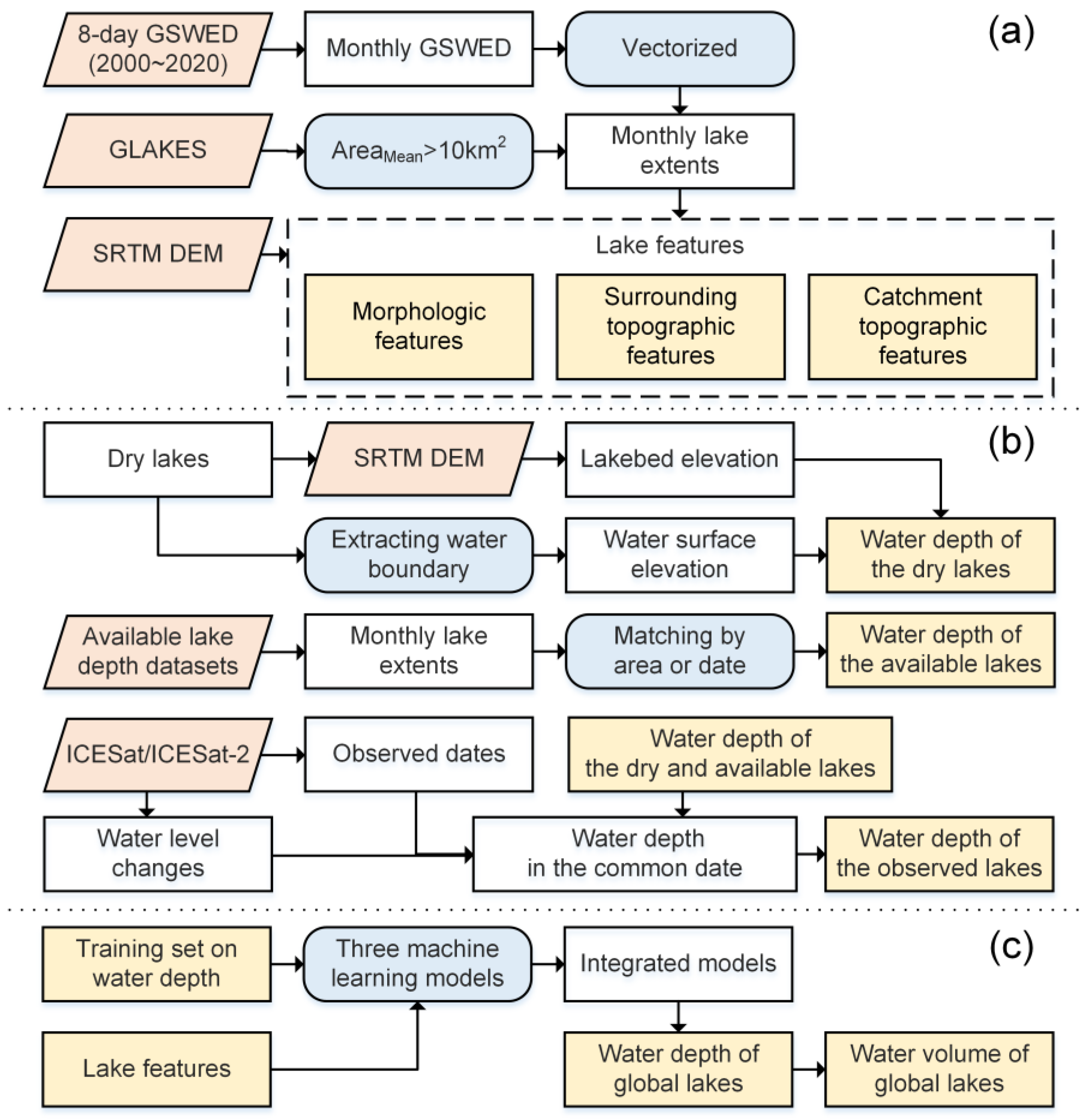
3.2. Monthly Global Lake Extents

The 8-day GSWED provides continuous and spatiotemporal surface water maps in 2000~2020, including the lake extents. The approach converted the 8-day data into monthly values and extracted the lake extents accordingly. Using the integration approach shown in Figure 2, a pixel was designated as water if it contained any water cover during a given month. After completing the processes including image mosaicking (where the initial images, downloaded from the website, have been segmented into equal regions), vectorization, and the selection of water features, this study derived the monthly global water surface extents in a refined vector format using ArcGIS Pro. To specifically isolate lake extents, the study employed the GLAKES dataset as a spatial mask, which was systematically intersected with monthly water surface extents. This spatial filtering process retained only those water bodies within the GLAKES boundaries as monthly lake extents, while effectively excluding non-lake water features including river systems, estuarine environments, coastal zones, and wetland marshes. The lake extents were identified consistently with the GLAKES dataset. Notably, lakes located at latitudes exceeding 60°N and 56°S or with surface areas smaller than 10 km² were excluded, as the elevation information from the SRTM DEM pertains only to the range between 56°S and 60°N.

3.3. Lake Features

In this study, we integrated previous findings and employed a variety of lake features (

Table 2. The detailed parameters of the lake features.

Features	Type	Unit	Description
Area	Morphologic features	km2	The surface area of a lake
Perimeter		km	The perimeter of a lake
SRatio		\	The ratio of the surface area and perimeter
Length		km	The range (maximum–minimum) of the longitude of a lake
Width		km	The range (maximum–minimum) of the latitude of a lake
LRatio		\	The ratio of the length and width
MeanS100	Surrounding topographic features	%	The mean slope in the 100 m buffer zone around a lake
Median S100		%	The median slope in the 100 m buffer zone around a lake
MaxS100		%	The maximum slope in the 100 m buffer zone around a lake
RangeS100		%	The range (maximum–minimum) of the slope in the 100 m buffer zone around a lake
STDS100		%	The standard deviation of the slope in the 100 m buffer zone around a lake
MeanHybas	Catchment topographic features	meter	The mean elevation in the hydrological basin where a lake is located
MedianHybas		meter	The median elevation in the hydrological basin where a lake is located
MaxHybas		meter	The maximum elevation in the hydrological basin where a lake is located
STDHybas		meter	The standard deviation of elevation in the hydrological basin where a lake is located

) as training and testing features for the ML models and took the monthly mean water depth of each lake as the target value. For the sake of conciseness, we used the term “morphological” to refer to the lake water surface and “topographic” to refer to the terrain surrounding a lake. The morphological features represent the size and shape of the free water surface, which indirectly reflect the lake water volume. The topographical features represent the elevation and terrain around the lake and in the catchment, which potentially affect the shape of the lakebed.

In detail, the morphological features include surface area, perimeter, the area–perimeter ratio (SRatio), length, width, and the length–width ratio (LRatio). The surface area and perimeter of a lake serve as indicators of its size, reflecting the capacity of a lake to hold water. The SRatio is a measure of the complexity of a lake water surface. A smaller ratio indicates simpler shapes, like circles or ellipses. The different ratios are caused by the terrain morphology, which determines the lake water depth. The length, width, and LRatio of a lake reflect a lake orientation. In general, tectonic lakes have larger length–width ratios and tend to be deeper, while volcanic lakes have a length–width ratio close to 1.

The surrounding topography determines the shape of the lakebed. For example, steep mountainous topography is often associated with deeper lakes (e.g., tectonic or glacial lakes), whereas shallower lakes, formed by wind or water erosion, are usually found in gently sloping plains. In addition, the surrounding topography indirectly affects lake volume and depth by influencing local climate (e.g., more precipitation on windward slopes, less on leeward slopes). Terrain morphology may reduce irradiance and therefore evaporation at a lake surface and maintain lake depth. A 100 m wide buffer zone around a lake boundary was defined and applied to calculate slope-related features. The latter included the following: mean slope (Mean_S100), median slope (Median_S100), maximum slope (Max_S100), slope range (Range_S100), and standard deviation of slope (STD_S100). The mean and median values reflect the average and intermediate values of the surrounding terrain slope, respectively. The mean is sensitive to extreme values, but it provides an overall representation of the terrain surrounding a water body. In contrast, the median is less affected by outliers. The maximum slope highlights the extreme values of the surrounding terrain slope, while the range and standard deviation capture the variability of the slope.

The topography of the catchment in which a lake is located affects the depth of the lake in a number of ways. A larger catchment area usually means that more precipitation is pooled into the lake, while a smaller catchment area may result in insufficient water inflow and a shallower lake. Steep terrain increases runoff and water inputs. Multiple topographic features of a lake catchment were used: mean (Mean_Hybas), median (Median_Hybas), and maximum elevation (Max_Hybas) and the standard deviation of elevation (STD_Hybas). The mean and median elevation values reflect the overall altitude of the catchment. The standard deviation of elevation measures the terrain ruggedness, aiding in the assessment of the spatial distribution of lake depth.

The parameters of area and perimeter are basic and well-known metrics and thus are not discussed further. We introduce two additional parameters: SRatio and LRatio, which are calculated as follows:

$$p=2 \sqrt{\mathrm{Area}\ast \pi }$$

(1)

$$\mathrm{SRatio}={\displaystyle \frac{Perimeter-p}{Perimeter+p}}$$

(2)

$$\mathrm{LRatio}={\displaystyle \frac{Length-Width}{Length+Width}}$$

(3)

where $p$ represents the equivalent perimeter of a lake, defined as the perimeter of a circle with the same area as the lake, and $Perimeter$ is the actual perimeter of the lake. Both ratio parameters are normalized: SRatio ranges from 0 to 1, and LRatio spans from −1 to 1. When SRatio is close to 0, the lake’s shape approximates a perfect circle. Conversely, as the SRatio increases, the shape becomes more irregular. A value of LRatio near −1 indicates a lake elongated in the north–south direction, whereas a value near 1 suggests a broader, east–west orientation.

As regards the topographic features in the surroundings of a lake, this study first estimated the slope for the entire SRTM DEM including the lake. This operation was carried out by applying the “Slope” tool in ArcGIS Pro. Then, the 100 m wide buffer zone around each monthly lake extent was applied as a mask to extract the slope values in the buffer zone and used to calculate the five topographic features. The five metrics were calculated with the “Zonal Statistics as Table” tool in ArcGIS Pro. The tool can summarize the statistical values of a raster within the zones of other data. Further, the catchment of each lake was determined according to the HydroBASINS Level 4 dataset. Then, the four indicators representing the catchment topographic features were likewise calculated by applying the “Zonal Statistics as Table” tool to the HydroBASINS and bare-earth SRTM DEM data.

3.4. Training Sets on Water Depth

This section introduces the three methods described in Figure 1b, which are used to generate water depth samples for training ML models.

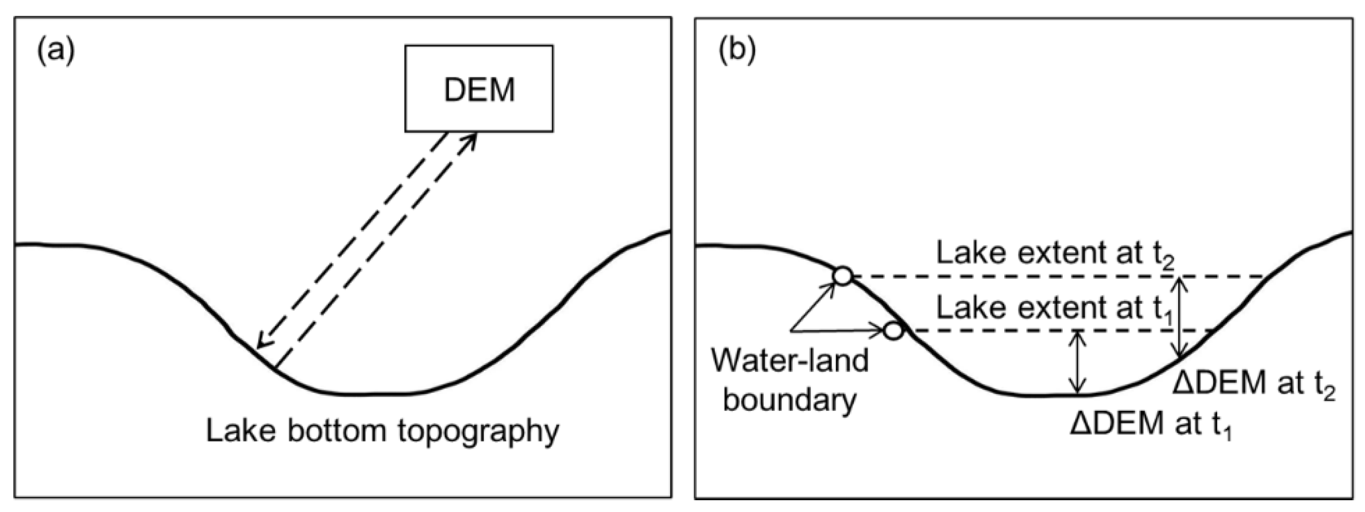
3.4.1. Training Set on the Dry Lakes

The water depth of so-called “dry lakes”, where lakebed elevations were exposed at a moment in time when a DEM could be generated and where the extent of the water surface was observed and delineated at any other time, can be calculated as the difference between the water level and lakebed elevations. This method has been validated in previous studies [56]. As shown in Figure 3, dry lakes (i.e., those with fully exposed lakebeds) were identified by comparing the lake extent images from February 2000 (the time when the SRTM DEM was acquired) with those from subsequent months. The SRTM DEM provides the elevation of these exposed lakebeds in February 2000. These elevations, combined with the vectorized monthly lake extents, were used to estimate the lake water surface elevation for each month between March 2000 and 2020. The estimation process involves the following steps: (1) converting the monthly lake water extents (polygons) into water boundary polylines; (2) creating a 30 m buffer zone around the water boundary; (3) using the ‘Zonal Statistics as Table’ tool in ArcGIS Pro to calculate the mean elevation values of the SRTM DEM within the buffer zone along the water boundary. The average elevation of the buffered water boundary serves as an estimate for the monthly lake water surface elevation, i.e., water level. Furthermore, estimates with significant inaccuracies in water boundaries (indicated by large standard deviations) would increase the uncertainty in water depth calculations. Considering that the elevations on the water boundary are nearly equal because the water surface is horizontal, a large standard deviation in the elevations on the water boundary pinpoints inaccuracies in the land–water boundary. To improve accuracy and reduce uncertainty, samples with water boundary elevation standard deviations exceeding 10 m were excluded.

Monthly maps of water surface elevations were generated following this methodology. For each month of inundation from March 2000 to December 2020, the water surface elevations were calculated on a pixel-wise basis. This involved subtracting the lakebed elevations in February 2000. Using this approach, a substantial global dataset on water depths was generated and utilized as training and testing samples. We calculated the monthly average water depth of the dry lakes as the training samples.

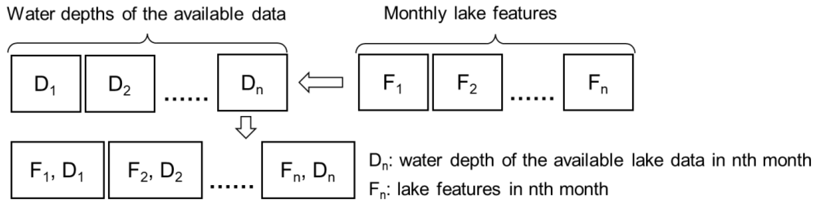
3.4.2. Training Set on the Available Lakes

Most available datasets provide only mean surface area and water depth values without temporal information, but they also offer valuable information improving the accuracy of water depth estimates. This study used the seven datasets introduced in Section 2.3. For the BathybaseDb, HydroLAKES, GLWD, GRanD, and ReGeom, and this study extracted the mean area and water depth values for special lakes. For the LWPED and WDFT, we obtained the water depth time series for several lakes in Asia and America. Due to the different geographical coverages and the unclear timestamps in the original data, these data need the necessary preprocessing and timestamp alignment.

BathybaseDb contains over 1200 lakes, providing their spatial extent and bathymetry in raster images but lacking clear timestamps. To address this, this study vectorized the raster images into polygons, extracted the geographical coordinates of each lake, and aligned them with the lake extents produced in Section 3.2. By calculating the average water depth and polygon area, this study estimated the surface area and mean water depth for each lake. Datasets such as HydroLAKES, GLWD, GRanD, and ReGeom offer precise spatial coordinates and polygons for lakes worldwide, along with attributes like average water depth and volume in lake shapefiles. However, these datasets lack temporal information, thus providing only static water depths. This study matched the lakes in these datasets with our lake extents based on their geographic location, then extracted their area and mean water depth. The LWPED dataset includes monthly in situ measurements from four lakes in China during 2016~2018, with multiple stations in each lake. This study assigned the same IDs to these lakes as in the lake extents, calculated the average water depth from the station data, and derived the monthly water depth for each lake during this period. The WDFT dataset provides in situ data with lake names, real-time surface areas, and volumes. Using Google Earth and the dataset’s published website, this study identified the corresponding lakes within our lake extents, then calculated the mean water depth by computing the ratio of water volume to surface area. The daily water depths were averaged to obtain the monthly water depths. Through these approaches, this study effectively organized the available data from multiple sources.

Although the available lake datasets, after preliminary processing, provide water depths for lakes, the absence of timestamps hinders their integration with dynamic lake features. To assign appropriate timestamps to the available data, this study adopted two matching approaches: one based on lake area and the other on available timestamps. The approach based on surface area assumes that a lake maintains a similar water depth under similar surface area conditions. As shown in Figure 4, the matching process based on the lake area involves the following steps:

(1)

extract the mean surface area and water depth of the target lake (A_t, D_t);

(2)

determine the monthly lake area from the lake extent data (A₁, A₂, … A_n);

(3)

identify the mth month where the lake area (A_m) most closely matches the mean area (A_t);

(4)

use the lake features and corresponding water depth for the mth month as a training sample (F_m, D_t).

Figure 4. The matching method for the available dataset based on lake area.

Figure 4. The matching method for the available dataset based on lake area.

This method was applied to datasets from BathybaseDb, GLWD, GRanD, HydroLAKES, and ReGeom. In contrast, the LWPED and WDFT datasets provide dynamic water depths. To synchronize these with the lake features, this study used the acquired timestamps to integrate the water depths with the corresponding lake features (listed in Table 2), as shown in Figure 5. The dynamic water depths (D_n) were subsequently aligned with the timestamps, generating feature-depth samples (F_n, D_n) for each timestamp. Notably, while the WDFT observations date back to the 1950s, this study focused only on the 2000~2020 period. Therefore, only the WDFT data within this timeframe were considered.

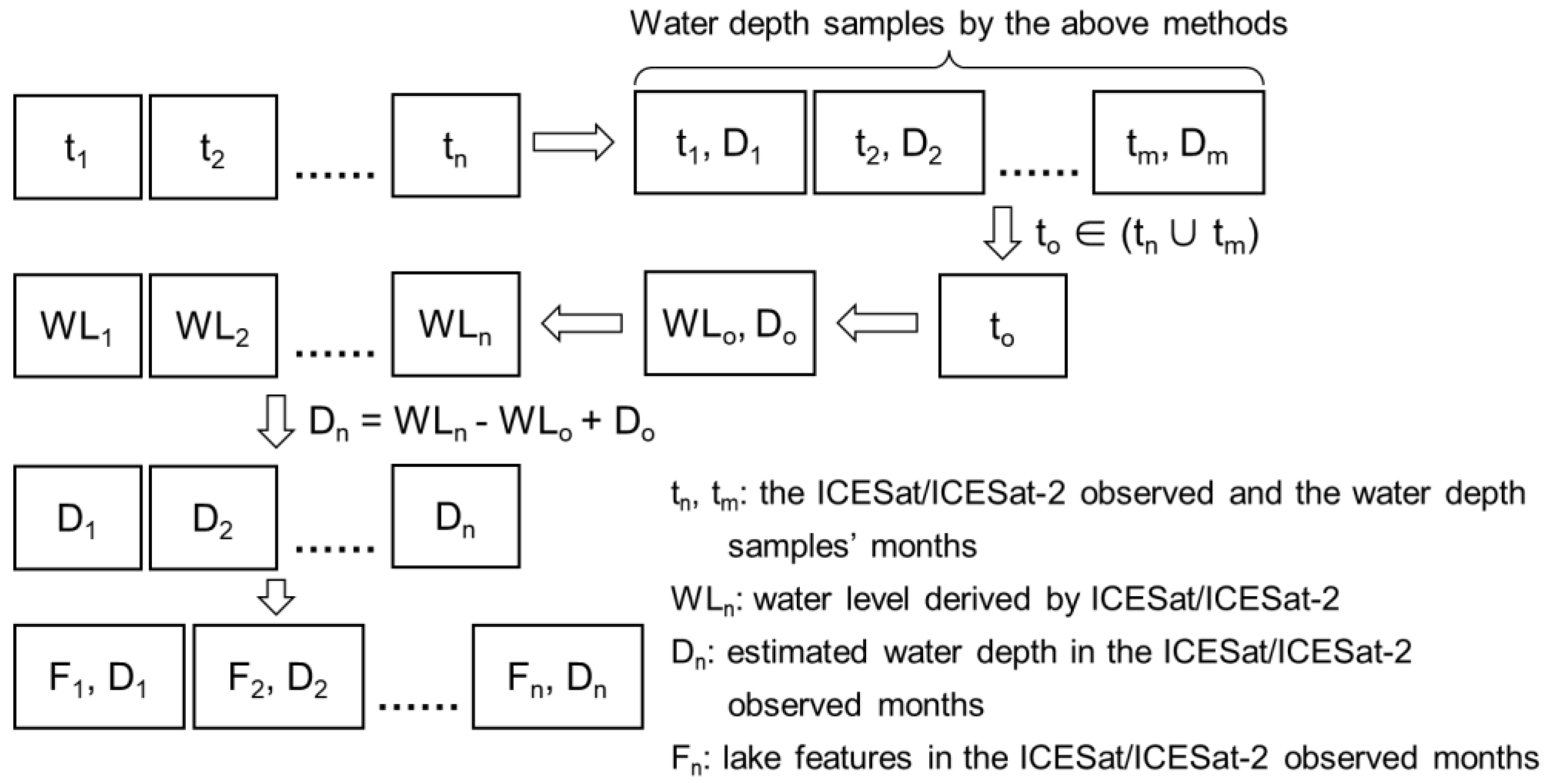
3.4.3. Training Set on the Lakes Observed by ICESat/ICESat-2

ICESat/ICESat-2 have demonstrated their ability to provide the remote sensing measurements of lake water levels [19,60,67]. Assuming negligible fluctuations in lakebed elevation, the lakebed elevation can be estimated as the difference between the lake water level and the water depth (if known):

$${\mathrm{WL}}_1-{\mathrm{WD}}_1={ \mathrm{WL}}_2-{\mathrm{WD}}_2=Lakebed elevation$$

(4)

$${\mathrm{WD}}_2={ \mathrm{WL}}_2-{\mathrm{WL}}_1+{\mathrm{WD}}_1$$

(5)

where ${\mathrm{WL}}_1$ and ${\mathrm{WL}}_2$ represent the water levels at different times, and ${\mathrm{WD}}_1$ and ${\mathrm{WD}}_2$ represent the water depths at corresponding times. Once the water depth is determined at a specific moment during ICESat/ICESat-2 observations, water depths at other observed times can be extrapolated using the recorded fluctuations in the water level. Therefore, this study operated under the assumption presented in the previous section, which posits that individual lakes maintain approximately equal water depths when subjected to the same or similar surface area conditions. A matching method for the ICESat/ICESat-2 observed lakes is illustrated in Figure 5. The monthly water levels of global lakes have been derived by processing the ICESat/ICESat-2 data, as detailed in Supplementary SA. As shown in Figure 6, the matching process can be divided into several steps:

(1)

determine in which months (t_n) the water level of a given lake was observed by ICESat/ICESat-2;

(2)

compare the observed months with the training sample months (t_m) generated by the previous methods, and identify the coincident months (t_o);

(3)

establish the corresponding water level from ICESat/ICESat-2 measurements and the water depth from the training sample for the coincident month (WL_o, D_o);

(4)

convert the ICESat/ICESat-2 water levels into water depths as a baseline (WL_o, D_o);

(5)

integrate the lake features (listed in Table 1) and water depths according to their timestamps to create new training samples (F_n, D_n).

Figure 6. The converting method for the water levels derived by ICESat/ICESat-2.

Figure 6. The converting method for the water levels derived by ICESat/ICESat-2.

4. Results and Analysis

4.1. Model Performance

4.1.1. Water Depth of the Global Dry Lakes

Figure 7 illustrates the global distribution and proportions of dry lakes relative to total lakes, highlighting significant regional disparities. Dry lakes account for ~7% of all lakes globally, amounting to 665 out of 8889 lakes. Their distribution is uneven across continents: Africa (~12.6%), Asia (~13.2%), and South America (~18.3%) exhibit significantly higher proportions of dry lakes, while Oceania (~9.3%), Europe (~3.7%), and North America (~1.7%) show much lower values. Dry lakes are concentrated in arid or semi-arid regions of the Northern Hemisphere, such as the western interior of North America (e.g., the “Great Basin” region of the United States), central Asia (e.g., northwestern China, Central Asia), and the Sahel region of Africa. These distribution patterns are likely influenced by regional climatic, topographic, and hydrological variations.

Despite accounting for a small proportion of global lakes, dry lakes hold considerable scientific significance. The dry lakes serve as key sources of water depth data during subsequent periods of inundation, as their exposed lakebeds allow for accurate elevation measurements. Using the estimation methods described in Section 3.4.1, this study extracted a substantial number of water depth samples from these regions, contributing to a better support for the water depth estimation.

This study also calculated the multi-year averages of their surface areas and the mean water depths of the dry lakes, as illustrated in Figure 8. The majority of dry lakes have a surface area of less than 100 km², and their mean water depths are predominantly below 4 m. These findings indicate that most dry lakes are medium or small sized. The accurate estimation of dry lake water depths provides valuable Supplementary Data to address the scarcity of field observations, particularly for small lakes. Field measurements for such lakes are limited, as they often receive less attention from researchers and organizations despite their widespread distribution. The scatterplot in Figure 8c illustrates the relationship between the multi-year averages of surface area and mean water depths for dry lakes. However, the analysis reveals no significant correlation to support the assumption that larger surface areas correspond to greater water depths. Small lakes can also exhibit relatively large water depths, undermining the reliability of estimating water depth based solely on surface area. This highlights the complex and multifaceted nature of the factors influencing the lakebed topography, even lake water depths, underscoring the need for further in-depth studies to understand these relationships.

The estimated water depths of the dry lakes play a crucial role in constructing the ML relationships, because they add key dynamic information into the training samples. Thus, the accuracy of these estimates directly impacts the performance of these relationships. As detailed in Section 3.4.1, the key to estimate the dynamic water depths of these lakes is the estimation of water levels. We used the water levels observed by ICESat/ICESat-2 as a reference to evaluate the estimated water levels. There are 763 ICESat/ICESat-2 observations (497 from ICESat and 266 from ICESat-2) and concurrent estimates based on our procedure. The results of the comparison (

Table 3. Comparative analysis of water levels observed by the ICESat\ICESat-2 and estimated by the water boundary method.

	Number	Bias (m)	MAE (m)	RMSE (m)	R2	KGE
ICESat	497	0.91	2.41	3.12	0.999	0.997
ICESat-2	266	2.10	3.35	5.35	0.999	0.996
Total	763	1.33	2.74	4.04	0.999	0.997

) are quite encouraging, e.g., an overall MAE of 2.74 m. Both the R² and KGE approach 1, indicating excellent performance. These results verify that the water levels estimated using the water boundary method align strongly with the ICESat\ICESat-2 observations. The estimated lake water depths are sufficiently reliable as a reference dataset to establish ML relationships applicable to all lakes.

4.1.2. Lake Training Samples

This study collected 76,030 training samples from 6472 lakes, representing approximately 73% of global lakes (Figure 9). Among these, a majority of the 56,976 samples (~75%) derived the estimated water depths of dry lakes. This method effectively addressed the gap in data for small and medium-sized lakes, which were often neglected in global lake studies and provided critical support to develop an empirical relationship to estimate lakebed elevation. In addition to the dry lake samples, the ICESat-derived method contributed 9424 samples, offering complementary dynamic water depth information. Together, these two methods supplied the majority of training samples, facilitating the modeling of lakes across all sizes. Moreover, available lake datasets, such as HydroLAKES (4145 samples), WDFT (3201 samples), and GRanD (1161 samples), contributed approximately 13% of the total samples (9630). These datasets were particularly valuable to estimate the lakebed elevations of large lakes. Although some lakes only have single-date samples that lack dynamic water depth information, they provide essential data that compensate the limitations of the dry lake approach. The integration of multiple data sources improved the spatial and geomorphological coverage of the lake training samples. Although the integration of multiple data sources might introduce uncertainties, these datasets contained valuable reference information that could not be ignored. Therefore, this study retained these datasets and leveraged their complementary strengths to improve the accuracy and robustness of the analysis. The training samples also exhibited a realistic distribution pattern, with a dominance of small lakes and relatively fewer large ones. The abundant and widely distributed training samples play a pivotal role in enhancing the performance and reliability of these models, particularly in improving water depth predictions for lakes of varying sizes.

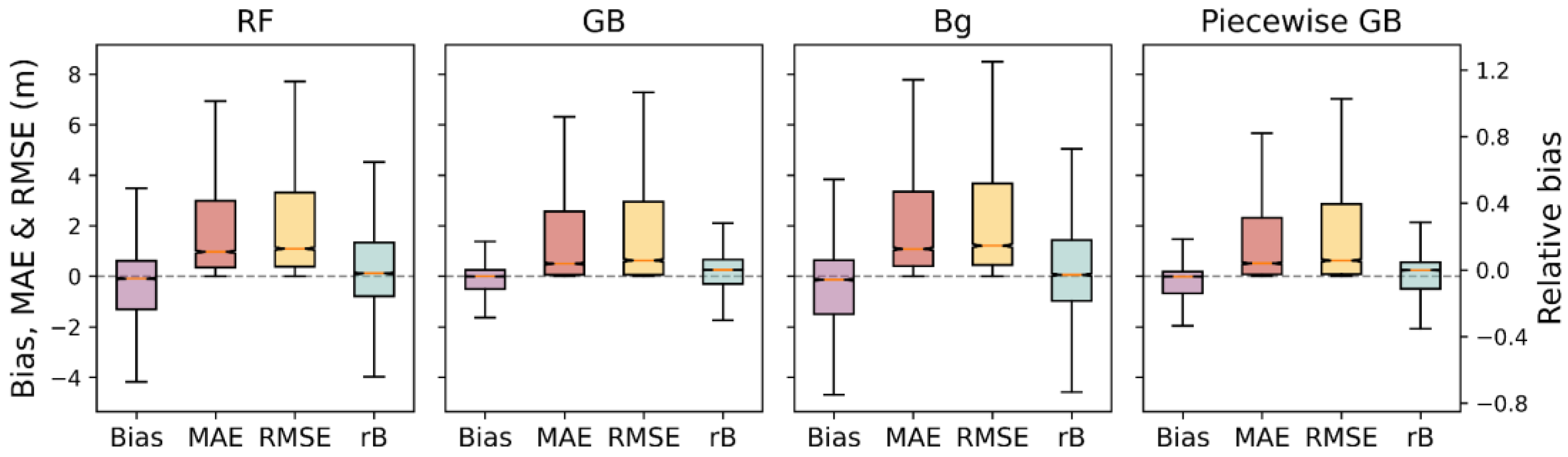
4.1.3. Reliability of ML Models

This study utilized a large water depth training dataset to explore the relationship between lake features and water depth using ML models. The original samples were randomly divided into a training set consisting of 80% of the original data and the remaining 20% was set aside as an independent testing set. The testing data were set as the reference to evaluate the estimates of lake water depths. To construct the ML relationships, we applied a hierarchical 5-fold cross-evaluation to the training set to optimize the hyperparameters of each of the three ML models. In addition, we applied thresholds to the maximum depth and the minimum number of splitting samples to reduce the model’s complexity and mitigate against overfitting. The grid search was applied to find the optimal parameters in each ML model with detailed information provided in Supplementary SC Table S1. After determining the optimal parameters, we applied the random segmentation to the testing samples five times to fully evaluate the performance of the relationships. Furthermore, a piecewise GB model was developed by the piecewise subsets of the training dataset. The piecewise subsets included samples with lake areas in the ranges of 0~1 km², 1~10 km², 10~10² km², 10²~10³ km², 10³~10⁴ km², and more than 10⁴ km² (noting that some lakes did not always maintain areas larger than 10 km²).

Table 4. The train and test mean performances of the three models.

	Number	Sample	Bias (m)	MAE (m)	RMSE (m)	R2	KGE
RF	76,030	train	0.01	0.45	1.99	0.99	0.97
		test	0.03	1.19	4.74	0.95	0.94
GB	76,030	train	−0.06	0.12	1.45	0.99	0.98
		test	−0.03	1.12	5.20	0.95	0.96
Bg	76,030	train	0.02	0.57	2.42	0.99	0.97
		test	0.06	1.24	4.77	0.95	0.94
Piecewise GB	76,030	train	−0.02	0.19	1.17	0.99	0.96
		test	−0.08	1.09	4.78	0.96	0.95
Piecewise GB (0~1 km2)	6672	train	−0.02	0.05	0.18	0.99	0.97
		test	0.01	0.44	0.81	0.39	0.51
Piecewise GB (1~10 km2)	26,251	train	−0.08	0.14	2.13	0.91	0.84
		test	−0.06	0.58	3.07	0.54	0.65
Piecewise GB (10~102 km2)	34,847	train	−0.09	0.17	1.74	0.97	0.94
		test	−0.10	1.22	4.97	0.76	0.82
Piecewise GB (102~103 km2)	6366	train	−0.09	0.16	1.07	0.99	0.97
		test	0.01	2.15	6.82	0.88	0.91
Piecewise GB (103~104 km2)	1502	train	−0.32	0.58	1.77	0.99	0.98
		test	−0.38	2.96	9.25	0.97	0.97
Piecewise GB (~104 km2)	392	train	−3.38	5.89	10.16	0.99	0.95
		test	−1.81	10.38	22.60	0.99	0.95

summarizes the average performance metrics of the three ML models under the five strategies and the total performance of the piecewise GB model, using metrics such as bias, MAE, RMSE, R², and KGE for both training and testing datasets. The detailed individual performance metrics of the three models under each splitting strategy are available in Supplementary SC Table S2. Additionally, scatterplots illustrating the comparison between the reference and predicted water depths for both training and testing datasets across the four models are presented in Figure 10. The compared scatterplots for the piecewise GB model in different lake area ranges are in Supplementary SC Figure S1.

The three ML methods demonstrated similar and outstanding performances in estimating water depth. In capturing the relationship between water depth and selected features, the models achieved average R² and KGE values near 1, showcasing their excellent ability to fit the data and explain the variation in mean water depth. In terms of error metrics, the biases were 0.01 m, −0.06 m, and 0.02 m; the MAEs were 0.45 m, 0.12 m, and 0.57 m; and the RMSEs were 1.99 m, 1.45 m, and 2.42 m. These results indicate that the models consistently produced low error rates compared to the training samples. Overall, the three models proved to be reliable and robust, offering strong support for accurate water depth predictions in future applications. The test performances of the three methods remained strong, with R² and KGE values also near 1. These results indicate that all methods effectively captured the relationship between lakebed elevation and lake features, even for the unknown water depth with no reference. In terms of error metrics, the biases were 0.03 m, −0.03 m, and 0.06 m; the MAEs were 1.19 m, 1.12 m, and 1.24 m; and the RMSEs were 4.74 m, 5.20 m, and 4.77 m. While the MAE values were satisfactory, the larger RMSE values suggest that predictions were generally accurate, but individual lakes exhibited larger errors. This discrepancy highlights the challenges in predicting water depths for certain lakes with specific conditions. Among the three methods, GB demonstrated the best overall performance, followed by RF, showcasing their robustness and adaptability to complex datasets. Although the performance on the test set was slightly worse than on the training set, the results underscored their strong generalization ability, delivering stable and accurate estimates across diverse datasets. Water depth, as a multifaceted attribute influenced by numerous factors, reflects the complexity of lake systems. The capability of ML algorithms to adapt to such intricate relationships proves to be a significant advantage, further affirming their suitability for large-scale water depth estimation.

Similarly, the assessment of the piecewise GB methods demonstrates their robust overall performance on both the training and testing samples in Table 4. For lakes across different area ranges, the models consistently achieved high R² values and KGE values, along with low biases, MAEs, and RMSEs, indicating their ability to accurately estimate known water depths. For the testing dataset, the models exhibited strong performance for lakes with areas larger than 10 km². Specifically, R² values were 0.76, 0.88, 0.97, and 0.99, and KGE values were 0.82, 0.91, 0.97, and 0.95 for lakes in the ranges of 10~10² km², 10²~10³ km², 10³~10⁴ km², and more than 10⁴ km², respectively. However, the performance significantly deteriorated for smaller lakes. For lakes with areas of 0~1 km² and 1~10 km², the R² values were only 0.39 and 0.54, and the KGE values dropped to 0.51 and 0.65, respectively. These results suggest that the piecewise GB models would provide uncertain estimations for smaller lakes. The reason will be discussed in Section 5.

4.2. Results and Assessment

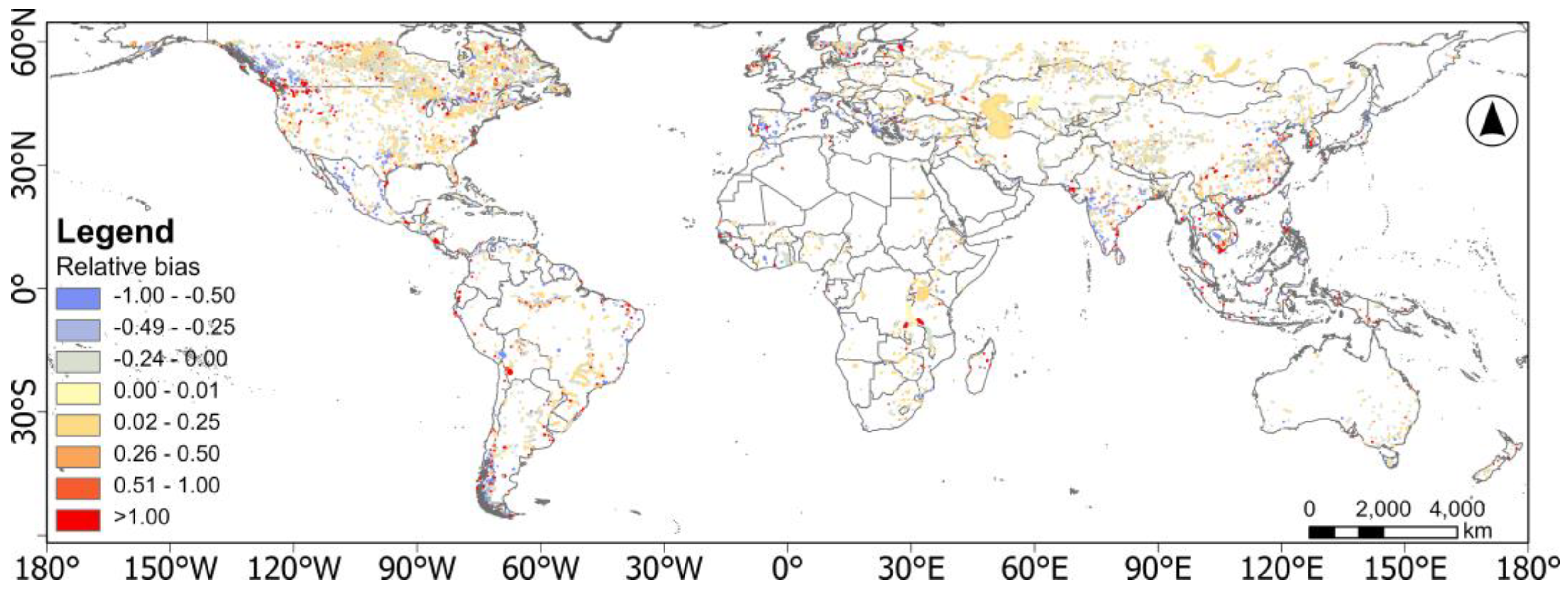
4.2.1. Assessment of the Individual Lakes

There are 6472 lakes which have water depths provided by the three generation methods. This section compares the estimates of the four models and the observed water depths wherever the latter were available. Figure 11 and Figure 12 presented the boxplots and spatial distributions of the performance metrics for the four methods. The results showed that the model performance on the individual lakes was consistent with the overall evaluation: the GB and the piecewise GB outperformed the other methods. The piecewise GB method achieved the best overall performance, with a lower bias, MAE, RMSE, and relative bias compared to the standard GB model. Specifically, the piecewise GB model achieved average values of −1.86 m (Bias), 3.59 m (MAE), 3.91 m (RMSE), and 0.27 (relative Bias), outperforming the standard GB model, which had values of −1.13 m, 3.69 m, 3.99 m, and 0.74, respectively. The superior performance of the piecewise GB model stemmed from its ability to capture the nuanced relationships between lake features and lakebed elevations across different lake size intervals. In particular, the piecewise GB model was effective in mitigating the disruption caused by the frequent oscillations in the water levels of small lakes compared with larger lakes. In contrast, the standard GB model struggled to fully describe these relationships without area-based segmentation. Based on these results, the piecewise GB model was selected as the final method of estimation, as it offers better adaptability to diverse lake characteristics and supports more accurate water depth estimation.

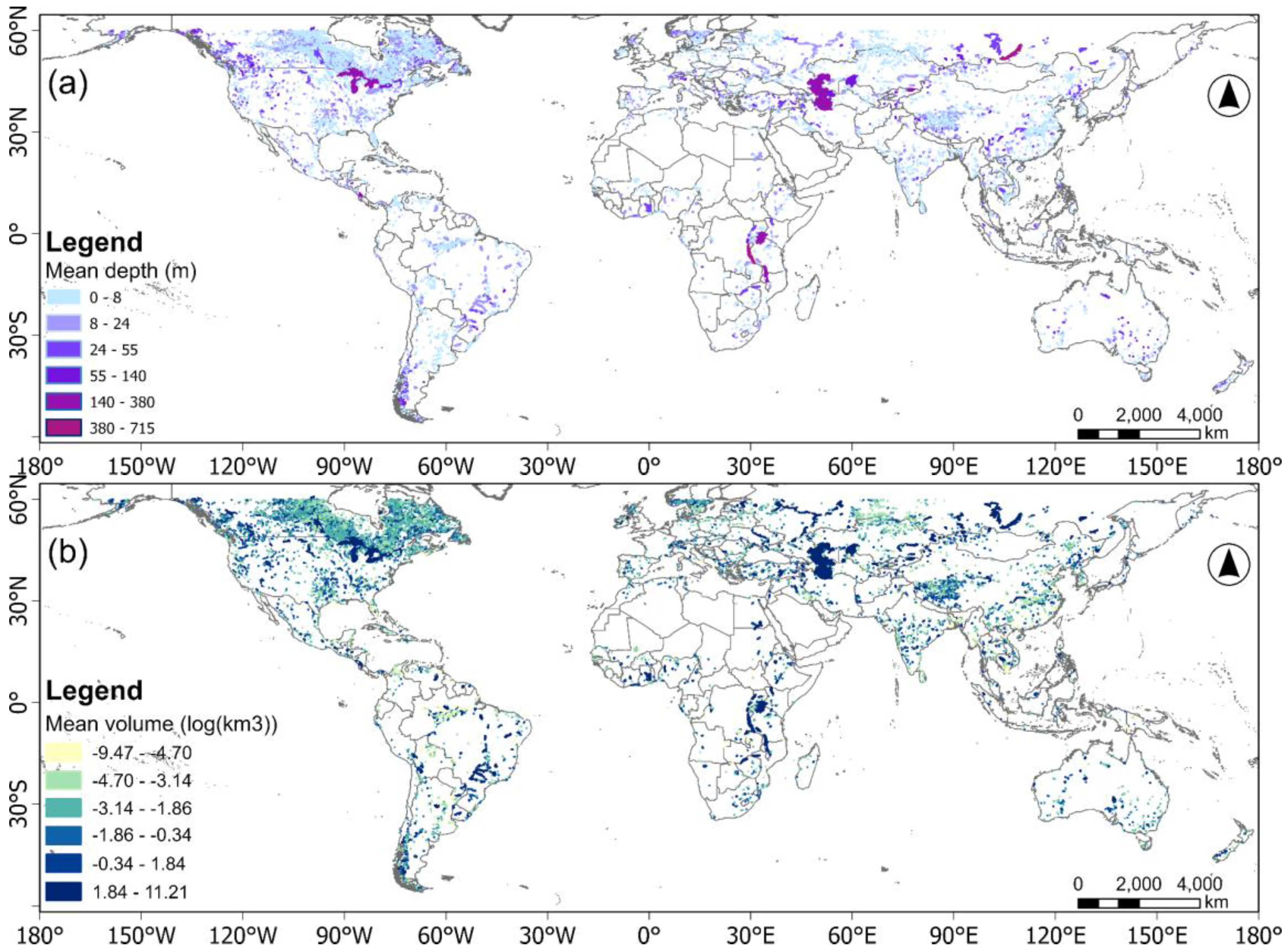
4.2.2. Estimated Water Depth

The monthly water volumes are calculated as the product of the lake area and the corresponding water depth for each month (Figure 13). According to the GLAKES database, the total area of the lakes analyzed in this study is ~1.628 million km², which accounts for about 85% of the total area of global natural lakes larger than 10 km² [16]. In terms of water depth distribution, the global lakes have an average water depth of 8.5 m and a median of 5.1 m. Notably, 951 lakes have a mean water depth of less than 1 m, while 6821 lakes have a mean water depth of less than 10 m, representing ~10.7% and ~72.6% of the total number of global lakes, respectively. This indicates that the majority of lakes worldwide have water depths ranging between 1 and 10 m. In addition, Supplementary SC Figure S2 illustrates the dynamic water depth of the selected lakes. This figure provides a visual representation of temporal changes, highlighting the methods’ capabilities to capture fluctuations in water depth over time.

In addition, the total water volume of global lakes is estimated to be approximately 188.5 × 10³ km³, which is about 8.0% higher than the ~174.2 × 10³ km³ reported by HydroLAKES. In terms of water volume distribution, the global lakes have an average water volume of 21.2 km³ and a median of 0.12 km³. Notably, 7676 lakes have water volumes of less than 1 km³, accounting for approximately 86.3% of the total number of global lakes but only ~0.63% of the total water volume. Similarly, 8619 lakes, representing ~97.0% of the total number of lakes, hold less than 10 km³ of water, contributing just ~2.12% of the global lake water volume. These findings highlight that while the majority of the global lake water volume is concentrated in large lakes, the widely distributed small and medium-sized lakes play a crucial complementary role in regulating water balance within regional catchments.

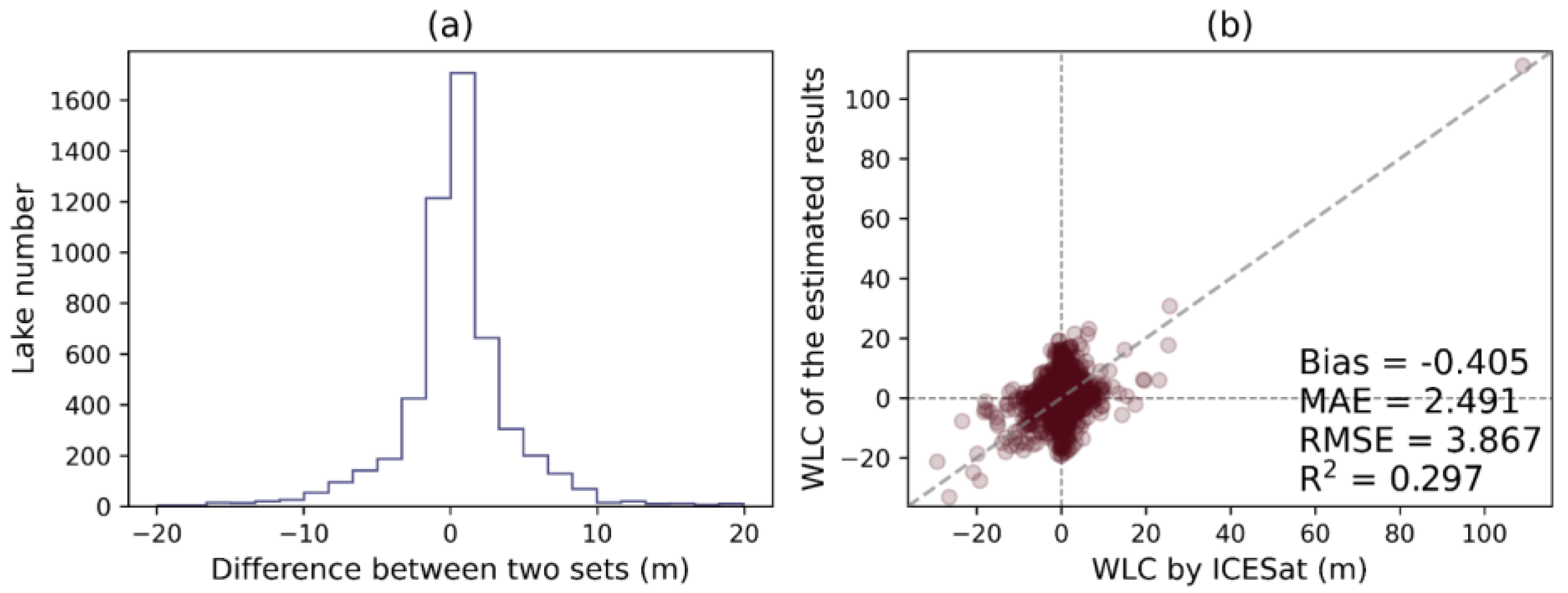
4.2.3. Comparison with the ICESat/ICESat-2 Observations

For the lakes with the ICESat/ICESat-2 observations, this study calculated the water level changes at the first and last observed months. Concurrently, the water depth changes in our estimates of those lakes at the coincident months (the first and last observed months of the ICESat/ICESat-2) were calculated as comparisons. The distribution of differences between the ICESat/ICESat-2 and our retrievals (Figure 14) is centered around zero, indicating that the majority of the differences are small. This suggests that while the model performs reasonably well overall, there are outliers where the discrepancies are more pronounced. Figure 13b provides a scatterplot comparing the estimated water depth changes with the ICESat water level changes for individual lakes. While many data points cluster around this line, some deviation is evident, particularly for larger change values. Key performance metrics are also presented: a bias of −0.405 m indicates a slight underestimation by the model on average. The MAE of 2.491 m and the RMSE of 3.867 m quantify the magnitude of errors, while the R² value of 0.297 reflects a moderate correlation between the estimates and ICESat/ICESat-2 observations. Overall, the figure highlights that our method obtains similar water depth changes with the ICESat/ICESat-2 observations.

This study further analyzed the monthly observation frequency (Figure 14) of ICESat and ICESat-2 over their operational periods (January 2003 to October 2009 for ICESat and September 2018 to December 2020 for ICESat-2), covering a total of 109 months. Given the sparse observations collected by these laser altimeters, larger lakes are more likely to receive frequent observations. To examine the quantitative frequency of observations, we categorized lakes by size and analyzed their observation frequencies, as shown in Figure 15. The results reveal a clear correlation between lake size and observation frequency. For lakes larger than 5000 km², the observation counts exceeded 10 times, with 42% (11 out of 26) being observed more than 55 times. The lake with the highest observation frequency was recorded 62 times, equivalent to ~57% of the total operational months of ICESat/ICESat-2. However, even for such large lakes, the data are not continuous, requiring time gaps to be filled. The situation is even worse for smaller lakes. Many lakes smaller than 5000 km² have significant gaps or even no observations. Notably, ~23% of the lakes within the 10~50 km² range were not observed at all, and ~96% of these lakes were observed no more than 11 times. This sparse observation frequency is insufficient for detailed analyses of water volume and depth changes in smaller lakes. By comparison, the water depths and volumes estimated by our model offer a significant advantage, as they achieve a temporal resolution comparable to that of optical satellites, enabling a more consistent and reliable analysis of lake dynamics.

4.3. Lake Feature Analysis

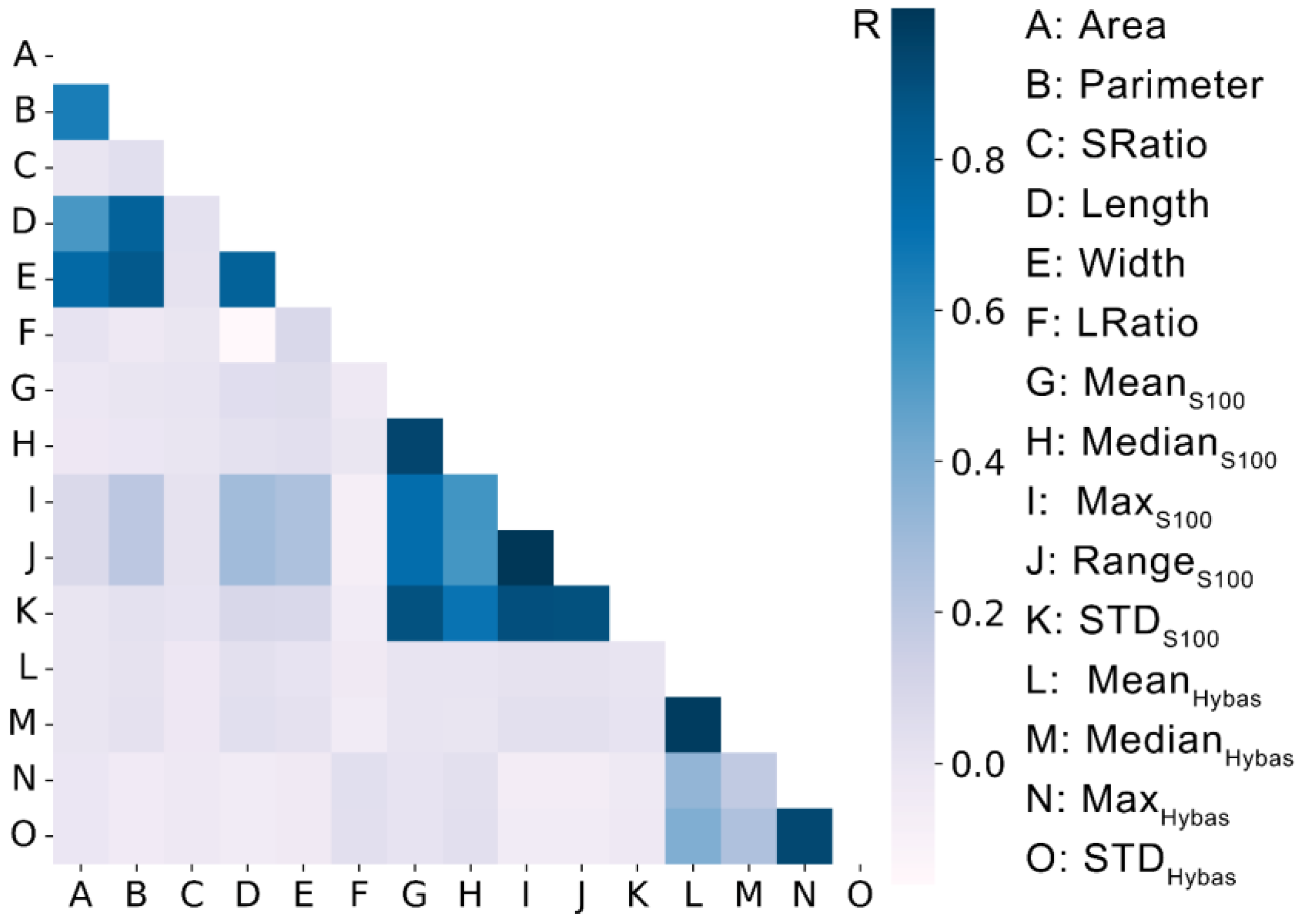
4.3.1. Feature Pairwise Correlations

The pairwise correlations among features were calculated to examine the relationships between them, as shown in Figure 16. The results indicate that most features exhibit low correlations with each other, highlighting their unique contributions. This diversity in lake features supports the construction of multidimensional relationships by ML methods. However, the same type of feature shows moderate to high correlations. For instance, lake area, perimeter, length, and width have pairwise correlations of approximately 0.7. Similarly, the statistical metrics of Mean_S100, Median_S100, Max_S100, Range_S100, and STD_S100 exhibit correlations around 0.9. Likewise, Mean_Hybas, Median_Hybas, Max_Hybas, and STD_Hybas have correlations near 0.7. This pattern aligns with traditional understanding, where larger lakes tend to have a greater area, perimeter, length, and width. Similarly, statistical values describing the topographical characteristics of the surrounding terrain or hydrological basin naturally correlate with each other. This is particularly important for capturing the multifaceted drivers of lakebed elevation, where different features may exhibit varying levels of importance depending on lake size, topography, or other conditions. Moreover, features with low correlations to others often provide unique and valuable information that enhances model performance and generalization. For instance, while features like lake area and perimeter are highly correlated, they may provide complementary information in describing different aspects of lake morphology. For example, when lakes are of the same area, lakes with longer perimeters are likely to have differences in lakebeds due to more complex surrounding topography. Similarly, the topographical features of the catchment may reveal patterns not captured by other variables. The next section on feature importance further elaborates on the relative contribution.

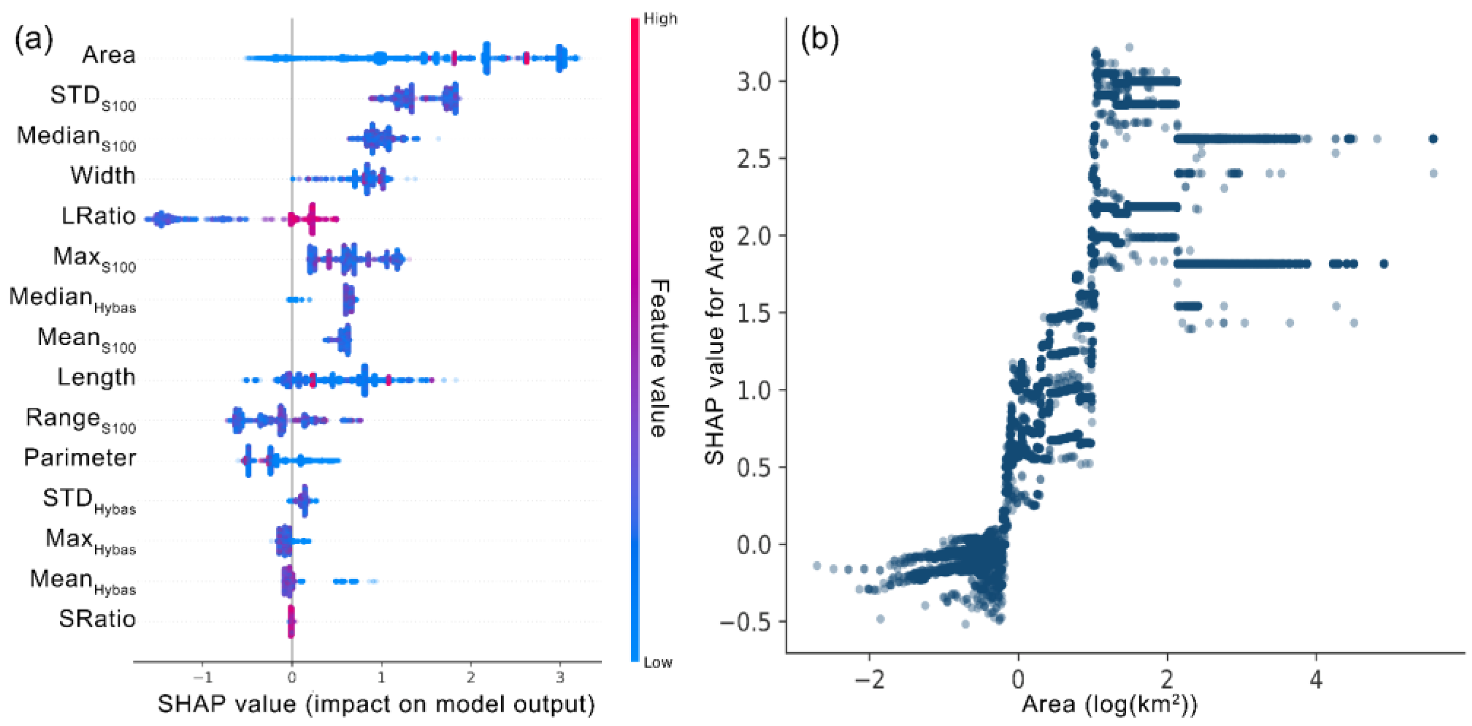
4.3.2. Feature Importance

To gain deeper insights into the significance and impact of various lake features, this study utilized SHapley Additive exPlanations (SHAP) to analyze the results obtained with the ML algorithms applied in the experiment. SHAP is a game-theory framework designed to interpret the outputs of ML algorithms. It links optimal credit allocation to local feature explanations by leveraging the classical Shapley values from game theory and their extended adaptations. For an ML model, the SHAP value measures the contribution of each feature to the model estimate, and SHAP decomposes the estimated value into the sum of the contributions of each feature, improving the transparency and consistency of interpretation [68,69].

To identify the key features influencing the GB model, SHAP values were analyzed and visualized across all samples (Figure 17). Features were ranked by the total magnitude of their SHAP values, reflecting their overall contribution to the estimated relationship. Among them, the lake area was the most significant predictor of lakebed elevation, though its relationship with water depth was nonlinear and complex, indicating interactions with other factors. The second and third most important features were the standard deviation and median of the elevation slopes around the lake, capturing terrain variability and general slope decline, respectively. Despite correlations between topographic features, each contributed unique information. Notably, the median slope had a greater impact than the mean, likely due to its robustness to outliers. In contrast, catchment topographic features were less influential, likely because of their long-term stability and limited variability. These features primarily served as contextual references, with a minimal direct impact on water depth estimates.

Further analysis of the influence of the lake area on the GB model’s predictions, as shown in Figure 17b, reveals a clear segmentation pattern with thresholds around 1 km², 10 km², and 10² km². This observation supports this study’s implementation of a piecewise GB relationship and aligns with previous research emphasizing stage-based relationships between lake area and water depth. For lakes in the 0~1 km² range, SHAP values generally increased with lake area, indicating a positive correlation. However, some samples displayed negative SHAP values, implying that additional, complex factors—such as local hydrological or topographical variability—may reduce the contribution of lake area to water depth estimates for smaller lakes. In the 1~10 km² range, SHAP values showed a steeper increase with lake area, demonstrating a strong positive influence of area on water depth predictions within this interval. For larger lakes (10~10² km² and more than 10² km²), SHAP values stabilized, indicating a consistent, albeit less pronounced, impact of lake area on estimates. Notably, the influence of lake area was slightly reduced for lakes larger than 10² km² compared to those in the 10~10² km² range, suggesting diminishing returns in its predictive power as the lake size increases further. This segmentation highlights the nonlinear and scale-dependent relationship between lake area and water depth, reinforcing the necessity of a piecewise modeling approach to better capture these dynamics across different lake size ranges.

The mean absolute SHAP values for each feature in the piecewise GB model are shown in Figure 18. In the area-based piecewise GB model, area characteristics are no longer the dominant influencing factors. Lakes of varying sizes exhibit different patterns of feature importance. For lakes smaller than 10 km², the median slope of the surrounding elevation emerges as the most important feature. In this context, we believe that the overall slope plays a crucial role. As the lake area increases to 10~10³ km², the maximum slope and the range of the slope become the most influential factors. These two metrics essentially represent the range of extreme slope values. For lakes of 10³~10⁴ km², the lake area becomes more significant. For lakes larger than 10⁴ km², the standard deviation of the slope ranks highest, followed by the mean slope. For smaller lakes with shorter shorelines, the range of slope extremes and variations is limited, meaning that the overall slope plays a more significant role in shaping the lake’s bottom topography. As the lake size increases and the shoreline lengthens, the range of terrain around the lake becomes more relevant, and the range of extreme slope values becomes more important than the overall slope. Finally, for very large lakes, greater variation in the surrounding terrain’s slope makes the standard deviation the most influential indicator. This finding will contribute to a better understanding of how the lake surface topography influences the formation and variation in the lakebed topography.

5. Discussion

5.1. Uncertainty in Small Lakes

Although the results and evaluation indicate that the proposed method achieves high accuracy for most lakes, some uncertainty remains, particularly for smaller lakes. According to Table 4 in Section 4.1.3, the piecewise GB model improves the R² values of 0.39 and 0.54, and the KGE values of 0.51 and 0.65, respectively, in the lakes with areas of 0~1 km² and 1~10 km². Several factors may contribute to the lower accuracy in small lakes. First, in many small lakes, there may be more anomalous relationships between lake features and water depth. The ML algorithm may overlook these specificities while identifying and interpreting general relationships, leading to errors. Second, the spatial resolution limitations of the surface water maps and the DEM data used in this study, along with the issue of mixed pixels caused by coarse resolution, are particularly problematic for small lakes. This may result in errors in the estimation and affect the relationships established by machine learning. Finally, smaller lakes typically have shallow water depths, and the inherent small errors in the method may be amplified in lakes with lower depths, further increasing relative bias.

5.2. Limitations of Surface Water Maps

Several global land surface water datasets are available, including the JRC GSWD [58] and the GSWED used in this study. The JRC GSWD provides lake water extent at 30 m spatial resolution, but with significant gaps in spatial and temporal coverage. The GSWED offers a seamless surface water map with 250 m of spatial resolution, that includes explicit classifications for ice and snow, effectively addressing the data gaps in frozen or snow-covered regions.

However, it is important to acknowledge the limitations of the GSWED. One key limitation is its spatial resolution of 250 m, which is considerably coarser than the 30 m resolution of the JRC GSWD. Lv et al. [56] showed that finer spatial resolution significantly improves the accuracy of water depth estimation, especially for small lakes. We hypothesize that the lower spatial resolution of the GSWED contributes to the reduced accuracy of the piecewise relationships when applied to small lakes compared to larger ones. Another limitation of the GSWED is its inability to distinguish whether ice and snow are located within the lake itself, a challenging but critical task. Although the study uses the GLAKES dataset to refine lake extents from the surface water data, it cannot differentiate dynamic lake extents that are covered by ice or snow. This limitation results in the loss of valuable dynamic information for lakes that are seasonally glaciated or snow-covered, thereby increasing the uncertainty in establishing the water depth estimator. Future advancements in surface water maps with finer spatial resolution and improved methods for identifying dynamic lake extents, including those influenced by ice and snow, are expected to significantly enhance the accuracy and reliability of water depth estimation models.

5.3. Applicability of the Methodology

The proposed method delivers dynamic estimates of lake water depth, but the temporal resolution is limited to one month by the GSWED satellite data products applied to delineate lake water surfaces. The monthly estimates of lake water depth are deemed sufficient to establish the required ML relationships. This implies that the proposed method cannot be applied for the real-time monitoring of lake water depth, since it is designed for long-term change and trend analysis.

6. Conclusions

The estimation of water depth and volume in global lakes has long been a complex and pressing challenge. Historically, only fragmented and approximate information about global lake depths and volumes has been available, with dynamic changes often inferred indirectly and partially through variations in lake water levels. The proposed method introduced an innovative sampling framework that generated comprehensive training datasets for ML models through multiple data approaches. This framework addressed two critical limitations of previous research: (1) it provided extensive coverage of lakes across all size categories, with emphasis on small and medium-sized lakes that were underrepresented in existing datasets; (2) it enabled continuous water depth estimation. The resulting dynamic estimates of global lake depth and volume represented a significant advancement in monitoring and managing lake water resources, particularly in response to climate change and anthropogenic impacts. Using these relationships, this study produced integrated monthly water depth and volume datasets for global lakes spanning 2000~2020. Accuracy evaluations and subsequent analyses demonstrate that the results provide reliable and essential data for advancing the analysis and management of global lakes.

The analysis highlights the varying importance and influence of different lake features on water depth. Among these, lake surface area emerges as the most critical factor, exhibiting a distinct piecewise relationship with thresholds at 1 km², 10 km², and 10² km². This finding justifies the adoption of a piecewise relationship in this study. Within each interval, surrounding topographic features, i.e., slopes around the lake, play a significant role in the estimation. For lakes smaller than 10 km², water depth is primarily influenced by localized topographic features, whereas larger lakes are more affected by the range of extreme slope values and standard deviation. Additionally, the median slope value proved more representative of general topographic trends than the mean slope value. In contrast, watershed-scale topographic features showed relatively low relevance and influence on water depth estimation.

While the research has achieved notable results, there is room for improvement. Due to computational constraints, this study primarily focused on lakes with surface areas exceeding 10 km². However, a vast number of smaller lakes, those less than 10 km² in area, are widely distributed across the globe. Expanding the method to dynamically estimate the water depth and volume for these smaller lakes remains a key objective. Furthermore, this study’s reliance on average water depth could be enhanced by acquiring pixel-wise bathymetry data, particularly for dry lakes. This finer-scale information would provide deeper insights into the lakebed topography. Future research will aim to address these limitations and advance the methodology further.

References

1. Yigzaw, W.; Li, H.Y.; Demissie, Y.; Hejazi, M.I.; Leung, L.R.; Voisin, N.; Payn, R. A New Global Storage-Area-Depth Data Set for Modeling Reservoirs in Land Surface and Earth System Models. Water Resour. Res. 2018, 54, 10372–10386. [Google Scholar] [CrossRef]
2. Messager, M.L.; Lehner, B.; Grill, G.; Nedeva, I.; Schmitt, O. Estimating the volume and age of water stored in global lakes using a geo-statistical approach. Nat. Commun. 2016, 7, 13603. [Google Scholar] [CrossRef]
3. Woolway, R.I.; Kraemer, B.M.; Lenters, J.D.; Merchant, C.J.; O’Reilly, C.M.; Sharma, S. Global lake responses to climate change. Nat. Rev. Earth Environ. 2020, 1, 388–403. [Google Scholar] [CrossRef]
4. Allen, G.H.; Pavelsky, T.M. Global extent of rivers and streams. Science 2018, 361, 585–588. [Google Scholar] [CrossRef]
5. Sobek, S. Predicting the depth and volume of lakes from map-derived parameters. Inland Waters 2011, 1, 177–184. [Google Scholar] [CrossRef]
6. Zhao, G.; Gao, H.; Cai, X. Estimating lake temperature profile and evaporation losses by leveraging MODIS LST data. Remote Sens. Environ. 2020, 251, 112104. [Google Scholar] [CrossRef]
7. Zhao, G.; Gao, H. Estimating reservoir evaporation losses for the United States: Fusing remote sensing and modeling approaches. Remote Sens. Environ. 2019, 226, 109–124. [Google Scholar] [CrossRef]
8. Obertegger, U.; Flaim, G.; Braioni, M.G.; Sommaruga, R.; Corradini, F.; Borsato, A. Water residence time as a driving force of zooplankton structure and succession. Aquat. Sci. 2007, 69, 575–583. [Google Scholar] [CrossRef]
9. Feng, Y.; Zhang, H.; Tao, S.; Ao, Z.; Song, C.; Chave, J.; Le Toan, T.; Xue, B.; Zhu, J.; Pan, J.; et al. Decadal Lake Volume Changes (2003–2020) and Driving Forces at a Global Scale. Remote Sens. 2022, 14, 1032. [Google Scholar] [CrossRef]
10. Grafton, R.Q.; Pittock, J.; Davis, R.; Williams, J.; Fu, G.; Warburton, M.; Udall, B.; McKenzie, R.; Yu, X.; Che, N.; et al. Global insights into water resources, climate change and governance. Nat. Clim. Change 2012, 3, 315–321. [Google Scholar] [CrossRef]
11. Verpoorter, C.; Kutser, T.; Seekell, D.A.; Tranvik, L.J. A global inventory of lakes based on high-resolution satellite imagery. Geophys. Res. Lett. 2014, 41, 6396–6402. [Google Scholar] [CrossRef]
12. Luo, S.; Song, C.; Ke, L.; Zhan, P.; Fan, C.; Liu, K.; Chen, T.; Wang, J.; Zhu, J. Satellite Laser Altimetry Reveals a Net Water Mass Gain in Global Lakes with Spatial Heterogeneity in the Early 21st Century. Geophys. Res. Lett. 2022, 49, e2021GL096676. [Google Scholar] [CrossRef]
13. Ma, Y.; Xu, N.; Liu, Z.; Yang, B.; Yang, F.; Wang, X.H.; Li, S. Satellite-derived bathymetry using the ICESat-2 lidar and Sentinel-2 imagery datasets. Remote Sens. Environ. 2020, 250, 112047. [Google Scholar] [CrossRef]
14. Liu, K.; Song, C.; Zhan, P.; Luo, S.; Fan, C. A Low-Cost Approach for Lake Volume Estimation on the Tibetan Plateau: Coupling the Lake Hypsometric Curve and Bottom Elevation. Front. Earth Sci. 2022, 10, 925944. [Google Scholar] [CrossRef]
15. Li, J.; Knapp, D.E.; Lyons, M.; Roelfsema, C.; Phinn, S.; Schill, S.R.; Asner, G.P. Automated Global Shallow Water Bathymetry Mapping Using Google Earth Engine. Remote Sens. 2021, 1, 1469. [Google Scholar] [CrossRef]
16. Pi, X.; Luo, Q.; Feng, L.; Xu, Y.; Tang, J.; Liang, X.; Ma, E.; Cheng, R.; Fensholt, R.; Brandt, M.; et al. Mapping global lake dynamics reveals the emerging roles of small lakes. Nat. Commun. 2022, 13, 5777. [Google Scholar] [CrossRef]
17. Pickens, A.H.; Hansen, M.C.; Hancher, M.; Stehman, S.V.; Tyukavina, A.; Potapov, P.; Marroquin, B.; Sherani, Z. Mapping and sampling to characterize global inland water dynamics from 1999 to 2018 with full Landsat time-series. Remote Sens. Environ. 2020, 243, 111792. [Google Scholar] [CrossRef]
18. Han, Q.; Niu, Z. Construction of the Long-Term Global Surface Water Extent Dataset Based on Water-NDVI Spatio-Temporal Parameter Set. Remote Sens. 2020, 12, 2675. [Google Scholar] [CrossRef]
19. Ma, S.; Liao, J.; Jing, R.; Chen, J. A dataset of lake level changes in China between 2002 and 2023 using multi-altimeter data. Big Earth Data 2024, 8, 166–188. [Google Scholar] [CrossRef]
20. Xu, N.; Ma, Y.; Zhang, W.; Wang, X.H. Surface-Water-Level Changes During 2003–2019 in Australia Revealed by ICESat/ICESat-2 Altimetry and Landsat Imagery. IEEE Geosci. Remote Sens. Lett. 2021, 18, 1129–1133. [Google Scholar] [CrossRef]
21. Luo, S.; Song, C.; Zhan, P.; Liu, K.; Chen, T.; Li, W.; Ke, L. Refined estimation of lake water level and storage changes on the Tibetan Plateau from ICESat/ICESat-2. Catena 2021, 200, 105177. [Google Scholar] [CrossRef]
22. Zhang, G.; Chen, W.; Xie, H. Tibetan Plateau’s Lake Level and Volume Changes from NASA’s ICESat/ICESat-2 and Landsat Missions. Geophys. Res. Lett. 2019, 46, 13107–13118. [Google Scholar] [CrossRef]
23. Qiao, B.; Zhu, L.; Wang, J.; Ju, J.; Ma, Q.; Huang, L.; Chen, H.; Liu, C.; Xu, T. Estimation of lake water storage and changes based on bathymetric data and altimetry data and the association with climate change in the central Tibetan Plateau. J. Hydrol. 2019, 578, 124052. [Google Scholar] [CrossRef]
24. Fang, Y.; Li, H.; Wan, W.; Zhu, S.; Wang, Z.; Hong, Y.; Wang, H. Assessment of Water Storage Change in China’s Lakes and Reservoirs over the Last Three Decades. Remote Sens. 2019, 11, 1467. [Google Scholar] [CrossRef]
25. Xie, J.; Li, B.; Jiao, H.; Zhou, Q.; Mei, Y.; Xie, D.; Wu, Y.; Sun, X.; Fu, Y. Water Level Change Monitoring Based on a New Denoising Algorithm Using Data from Landsat and ICESat-2: A Case Study of Miyun Reservoir in Beijing. Remote Sens. 2022, 14, 4344. [Google Scholar] [CrossRef]
26. Mateo-Pérez, V.; Corral-Bobadilla, M.; Ortega-Fernández, F.; Vergara-González, E.P. Port Bathymetry Mapping Using Support Vector Machine Technique and Sentinel-2 Satellite Imagery. Remote Sens. 2020, 12, 2069. [Google Scholar] [CrossRef]
27. Yang, H.; Guo, H.; Dai, W.; Nie, B.; Qiao, B.; Zhu, L. Bathymetric mapping and estimation of water storage in a shallow lake using a remote sensing inversion method based on machine learning. Int. J. Digit. Earth 2022, 15, 789–812. [Google Scholar] [CrossRef]
28. Lehner, B.; Liermann, C.R.; Revenga, C.; Vörösmarty, C.; Fekete, B.; Crouzet, P.; Döll, P.; Endejan, M.; Frenken, K.; Magome, J.; et al. High-resolution mapping of the world’s reservoirs and dams for sustainable river-flow management. Front. Ecol. Environ. 2011, 9, 494–502. [Google Scholar] [CrossRef]
29. Caballero, I.; Stumpf, R.P. Retrieval of nearshore bathymetry from Sentinel-2A and 2B satellites in South Florida coastal waters. Estuar. Coast. Shelf Sci. 2019, 226, 106277. [Google Scholar] [CrossRef]
30. Tsolakidis, I.; Vafiadis, M. Comparison of Hydrographic Survey and Satellite Bathymetry in Monitoring Kerkini Reservoir Storage. Environ. Process. 2019, 6, 1031–1049. [Google Scholar] [CrossRef]
31. Wan, J.; Ma, Y. Shallow Water Bathymetry Mapping of Xinji Island Based on Multispectral Satellite Image using Deep Learning. J. Indian Soc. Remote Sens. 2021, 49, 2019–2032. [Google Scholar] [CrossRef]
32. Yang, N.; Li, J.H.; Mo, W.B.; Luo, W.J.; Wu, D.; Gao, W.C.; Sun, C.H. Water depth retrieval models of East Dongting Lake, China, using GF-1 multi-spectral remote sensing images. Glob. Ecol. Conserv. 2020, 22, e01004. [Google Scholar] [CrossRef]
33. Qi, M.; Liu, S.; Wu, K.; Zhu, Y.; Xie, F.; Jin, H.; Gao, Y.; Yao, X. Improving the accuracy of glacial lake volume estimation: A case study in the Poiqu basin, central Himalayas. J. Hydrol. 2022, 610, 127973. [Google Scholar] [CrossRef]
34. Qiao, B.; Ju, J.; Zhu, L.; Chen, H.; Kai, J.; Kou, Q. Improve the Accuracy of Water Storage Estimation—A Case Study from Two Lakes in the Hohxil Region of North Tibetan Plateau. Remote Sens. 2021, 13, 293. [Google Scholar] [CrossRef]
35. Gu, Z.; Zhang, Y.; Fan, H. Mapping inter- and intra-annual dynamics in water surface area of the Tonle Sap Lake with Landsat time-series and water level data. J. Hydrol. 2021, 601, 126644. [Google Scholar] [CrossRef]
36. Haakanson, L.; Peters, R.H. Predictive Limnology: Methods for Predictive Modelling; Wiley: Hoboken, NJ, USA, 1995. [Google Scholar] [CrossRef]
37. Håkanson, L.; Karlsson, B. On the Relationship between Regional Geomorphology and Lake Morphometry—A Swedish Example. Geogr. Ann. Ser. A Phys. Geogr. 1984, 66, 103–119. [Google Scholar] [CrossRef]
38. Heathcote, A.J.; del Giorgio, P.A.; Prairie, Y.T.; Brickman, D. Predicting bathymetric features of lakes from the topography of their surrounding landscape. Can. J. Fish. Aquat.Sci. 2015, 72, 643–650. [Google Scholar] [CrossRef]
39. Cai, X.; Gan, W.; Ji, W.; Zhao, X.; Wang, X.; Chen, X. Optimizing Remote Sensing-Based Level–Area Modeling of Large Lake Wetlands: Case Study of Poyang Lake. IEEE J. Sel. Top. Appl. Earth Obs. Remote Sens. 2015, 8, 471–479. [Google Scholar] [CrossRef]
40. Hollister, J.W.; Milstead, W.B.; Urrutia, M.A. Predicting maximum lake depth from surrounding topography. PLoS ONE 2011, 6, e25764. [Google Scholar] [CrossRef]
41. Hollister, J.; Milstead, W.B. Using GIS to estimate lake volume from limited data. Lake Reserv. Manag. 2010, 26, 194–199. [Google Scholar] [CrossRef]
42. Lehner, B.; Döll, P. Development and validation of a global database of lakes, reservoirs and wetlands. J. Hydrol. 2004, 296, 1–22. [Google Scholar] [CrossRef]
43. Delaney, C.; Li, X.; Holmberg, K.; Wilson, B.; Heathcote, A.; Nieber, J. Estimating Lake Water Volume with Regression and Machine Learning Methods. Front. Water 2022, 4, 886964. [Google Scholar] [CrossRef]
44. Muñoz, R.; Huggel, C.; Frey, H.; Cochachin, A.; Haeberli, W. Glacial lake depth and volume estimation based on a large bathymetric dataset from the Cordillera Blanca, Peru. Earth Surf. Process. Landf. 2020, 45, 1510–1527. [Google Scholar] [CrossRef]
45. Fair, Z.; Flanner, M.; Brunt, K.M.; Fricker, H.A.; Gardner, A. Using ICESat-2 and Operation IceBridge altimetry for supraglacial lake depth retrievals. Cryosphere 2020, 14, 4253–4263. [Google Scholar] [CrossRef]
46. Weekley, D.; Li, X. Tracking lake surface elevations with proportional hypsometric relationships, Landsat imagery, and multiple DEMs. Water Resour. Res. 2021, 57, e2020WR027666. [Google Scholar] [CrossRef]
47. Weekley, D.; Li, X. Tracking Multidecadal Lake Water Dynamics with Landsat Imagery and Topography/Bathymetry. Water Resour. Res. 2019, 55, 8350–8367. [Google Scholar] [CrossRef]
48. Yang, H.; Qiao, B.; Huang, S.; Fu, Y.; Guo, H. Fitting profile water depth to improve the accuracy of lake depth inversion without bathymetric data based on ICESat-2 and Sentinel-2 data. Int. J. Appl. Earth Obs. Geoinf. 2023, 119, 103310. [Google Scholar] [CrossRef]
49. Xu, N.; Ma, Y.; Zhou, H.; Zhang, W.; Zhang, Z.; Wang, X.H. A Method to Derive Bathymetry for Dynamic Water Bodies Using ICESat-2 and GSWD Data Sets. IEEE Geosci. Remote Sens. Lett. 2022, 19, 1–5. [Google Scholar] [CrossRef]
50. Li, Y.; Gao, H.; Zhao, G.; Tseng, K.-H. A high-resolution bathymetry dataset for global reservoirs using multi-source satellite imagery and altimetry. Remote Sens. Environ. 2020, 244, 111831. [Google Scholar] [CrossRef]
51. Armon, M.; Dente, E.; Shmilovitz, Y.; Mushkin, A.; Cohen, T.J.; Morin, E.; Enzel, Y. Determining Bathymetry of Shallow and Ephemeral Desert Lakes Using Satellite Imagery and Altimetry. Geophys. Res. Lett. 2020, 47, e2020GL087367. [Google Scholar] [CrossRef]
52. Fang, C.; Lu, S.; Li, M.; Wang, Y.; Li, X.; Tang, H.; Odion Ikhumhen, H. Lake water storage estimation method based on similar characteristics of above-water and underwater topography. J. Hydrol. 2023, 618, 129146. [Google Scholar] [CrossRef]
53. Liu, K.; Song, C. Modeling lake bathymetry and water storage from DEM data constrained by limited underwater surveys. J. Hydrol. 2022, 604, 127260. [Google Scholar] [CrossRef]
54. Bemmelen, C.W.T.; Mann, M.; Ridder, M.P.; Rutten, M.M.; Giesen, N.C. Determining water reservoir characteristics with global elevation data. Geophys. Res. Lett. 2016, 43, 1–11. [Google Scholar] [CrossRef]
55. Liu, K.; Song, C.; Zhao, S.; Wang, J.; Chen, T.; Zhan, P.; Fan, C.; Zhu, J. Mapping inundated bathymetry for estimating lake water storage changes from SRTM DEM: A global investigation. Remote Sens. Environ. 2024, 301, 113960. [Google Scholar] [CrossRef]
56. Lv, Y.; Jia, L.; Menenti, M.; Zheng, C.; Jiang, M.; Lu, J.; Zeng, Y.; Chen, Q.; Bennour, A. A novel remote sensing method to estimate pixel-wise lake water depth using dynamic water-land boundary and lakebed topography. Int. J. Digit. Earth 2024, 17, 2440443. [Google Scholar] [CrossRef]
57. O’Loughlin, F.E.; Paiva, R.C.D.; Durand, M.; Alsdorf, D.E.; Bates, P.D. A multi-sensor approach towards a global vegetation corrected SRTM DEM product. Remote Sens. Environ. 2016, 182, 49–59. [Google Scholar] [CrossRef]
58. Pekel, J.F.; Cottam, A.; Gorelick, N.; Belward, A.S. High-resolution mapping of global surface water and its long-term changes. Nature 2016, 540, 418–422. [Google Scholar] [CrossRef]
59. Yamazaki, D.; Ikeshima, D.; Tawatari, R.; Yamaguchi, T.; O’Loughlin, F.; Neal, J.C.; Sampson, C.C.; Kanae, S.; Bates, P.D. A high-accuracy map of global terrain elevations. Geophys. Res. Lett. 2017, 44, 5844–5853. [Google Scholar] [CrossRef]
60. Zhan, P.; Song, C.; Luo, S.; Liu, K.; Ke, L.; Chen, T. Lake Level Reconstructed from DEM-Based Virtual Station: Comparison of Multisource DEMs with Laser Altimetry and UAV-LiDAR Measurements. IEEE Geosci. Remote Sens. Lett. 2022, 19, 1–5. [Google Scholar] [CrossRef]
61. Geurts, P.; Ernst, D.; Wehenkel, L. Extremely randomized trees. Mach. Learn. 2006, 63, 3–42. [Google Scholar] [CrossRef]
62. Breiman, L. Random Forests. Mach. Learn. 2001, 45, 5–32. [Google Scholar] [CrossRef]
63. Demiriz, A.; Bennett, K.P.; Shawe-Taylor, J. Linear Programming Boosting via Column Generation. Mach. Learn. 2002, 46, 225–254. [Google Scholar] [CrossRef]
64. Friedman, J.H. Stochastic gradient boosting. Comput. Stat. Data Anal. 2002, 38, 367–378. [Google Scholar] [CrossRef]
65. Ho, T.K. The Random Subspace Method for Constructing Decision Forests. IEEE Trans. Pattern Anal. Mach. Intell. 1998, 20, 832–844. [Google Scholar]
66. Breiman, L. Bagging Predictors. Mach. Learn. 1996, 24, 123–140. [Google Scholar] [CrossRef]
67. Zou, F.; Tenzer, R.; Jin, S. Water Storage Variations in Tibet from GRACE, ICESat, and Hydrological Data. Remote Sens. 2019, 11, 1103. [Google Scholar] [CrossRef]
68. Aas, K.; Jullum, M.; Løland, A. Explaining individual predictions when features are dependent: More accurate approximations to Shapley values. Artif. Intell. 2021, 298, 103502. [Google Scholar] [CrossRef]
69. Lundberg, S.M.; Lee, S.I. A Unified Approach to Interpreting Model Predictions. In Proceedings of the 31st Conference on Neural Information Processing Systems (NIPS 2017), Long Beach, CA, USA, 22 May 2017. [Google Scholar]
70. Shen, C.; Jia, L.; Ren, S. Inter- and Intra-Annual Glacier Elevation Change in High Mountain Asia Region Based on ICESat-1&2 Data Using Elevation-Aspect Bin Analysis Method. Remote Sens. 2022, 14, 1630. [Google Scholar] [CrossRef]
71. Huang, T.; Jia, L.; Menenti, M.; Lu, J.; Zhou, J.; Hu, G. A New Method to Estimate Changes in Glacier Surface Elevation Based on Polynomial Fitting of Sparse ICESat-GLAS Footprints. Sensors 2017, 17, 1803. [Google Scholar] [CrossRef]
72. Gupta, H.V.; Kling, H. On typical range, sensitivity, and normalization of Mean Squared Error and Nash-Sutcliffe Efficiency type metrics. Water Resour. Res. 2011, 47. [Google Scholar] [CrossRef]
Figure 1. The flowchart of the proposed method: (a) computing the lake features, (b) generating the training sets on water depth, and (c) building the relationship by ML between the candidate features and water depth to estimate the water depth and volume of global lakes. The red boxes are the input data, the blue boxes are the key processing, and the yellow boxes are the productions and results during the method.
Remotesensing 17 01052 g001
Figure 2. The method for integrating the 8-day images into monthly images during 2000~2020.
Remotesensing 17 01052 g002
Figure 3. The concept for extracting water depth from the dry lakes during 2000~2020. (a) the lakebed elevations, if exposed, can be completely determined using a DEM; (b) the elevations along water-land boundary at time t1 and t2 are determined using the same DEM to estimate the elevation of the water surface.
Remotesensing 17 01052 g003
Figure 5. The matching method for the available dataset based on the acquired timestamps.
Remotesensing 17 01052 g005
Figure 7. The distributions and numbers of the global dry lakes: (a) is the spatial distribution of the global dry lakes, (b) is the number of the dry and total lakes in each continent, and (c) is the ratio of the dry lakes in global lakes.
Remotesensing 17 01052 g007
Figure 8. The multi-year averages of the surface areas and the mean water depths of the global dry lakes: (a) is the multi-year averages of the surface areas of dry lakes in each continent, (b) is the multi-year averages of the mean water depth statistics of dry lakes in each continent, and (c) is the relationship between the multi-year averages of the surface area and the mean water depths of the dry lakes. The different colors represent the different continents. The abridges of continents are as follows: Af is Africa, As is Asia, Eu is Europe, NA is North America, Oc is Oceania, and SA is South America.
Remotesensing 17 01052 g008
Figure 9. The sources of data, water depth, and lake area of lake training samples: (a) is the sources of data, (b) is the distributions of water depth, and (c) is the distributions of lake area (“+” represents the outliers beyond the caps). The ticks in the x axis represent: D (dry lakes), I (ICESat/ICESat-2), H (HydroLAKES), W (WDFT), G (GRanD), R (ReGeom), L (LWPED), GL (GLWD), and B (BathybaseDb).
Remotesensing 17 01052 g009
Figure 10. Scatterplots of the referenced and predicted water depth from the training and testing datasets with three ML models.
Remotesensing 17 01052 g010
Figure 11. The boxplots of the performance metrics of the three methods and the piecewise GB method in each assessed lake.
Remotesensing 17 01052 g011
Figure 12. The relative bias between the reference and estimated water depths in each lake during 2000~2020.
Remotesensing 17 01052 g012
Figure 13. The mean water depth (a) and volume (b) of global lakes during 2000~2020 estimated with the piecewise GB methods.
Remotesensing 17 01052 g013
Figure 14. The histogram (a) of the difference between the water level changes derived by ICESat/ICESat-2 and the water depth changes in the estimated results and the scatter (b) between the two sets.
Remotesensing 17 01052 g014
Figure 15. The observed frequency (a) and ratio (b) of ICESat/ICESat-2 in different-sized lakes at the monthly scale during 2000~2020 (January 2003~October 2009 and September 2018~December 2020). “--” represents no observation of ICESat/ICESat-2.
Remotesensing 17 01052 g015
Figure 16. The pairwise correlations of each feature.
Remotesensing 17 01052 g016
Figure 17. The SHAP values for (a) each feature and (b) lake area in the GB model.
Remotesensing 17 01052 g017
Figure 18. The mean absolute SHAP values for each feature in the piecewise GB model: (a) 0~1 km2, (b) 1~10 km2, (c) 10~102 km2, (d) 102~103 km2, (e) 103~104 km2, and (f) more than 104 km2.
Remotesensing 17 01052 g018