Extinction Coefficient Inversion Algorithm with New Boundary Value Estimation for Horizontal Scanning Lidar

Abstract

Lidar has been used for many years to study the optical properties of aerosols, but estimating the boundary values requires solving the lidar elastic scattering equation, which remains a challenge. The boundary values are often determined by fitting to uniform regions of the atmosphere. This method typically excludes low signal-to-noise ratio (SNR) signals because it classifies them as non-uniform, reducing the effective detection range of the lidar. On the other hand, directly fitting low SNR signals to estimate the boundary values can introduce significant errors. The method is based on maximizing the lidar detection distance and determines the boundary value using a new estimation algorithm with the averaging of multiple fitted results in the low SNR region to reduce the impact of noise. Simulations demonstrate that the new method reduces the relative error in the boundary value estimation by approximately 5% and improves the accuracy of the extinction coefficient profile inversion compared with the method of directly fitting all-sample signals. Field comparison experiments with forward-scattering sensors further verify that the algorithm improves the retrieval accuracy by 17.3% under extremely low signal-to-noise ratio (SNR) conditions, while performing comparably to the traditional method in high SNR homogeneous atmospheres. Additionally, based on the scanned lidar signals, the algorithm can provide detailed information on the spatial distribution of sea fog and offer valuable insights for an in-depth understanding of the physical evolution of sea fog.

1. Introduction

Aerosols significantly influence atmospheric clouds and precipitation [1,2], visibility [3], and the radiation budget [4], and they play an extremely important role in weather and climate change. Aerosol optical properties are subject to large diversity, because of the abundance and variety of sources and the complexity of meteorological processes, which results in wide variations of physical properties and chemical compositions [5]. To gain an in-depth understanding of aerosol optical properties and processes, high-precision and long-term continuous observations are required. With the advantages of high temporal and spatial resolution, lidar has become a major instrument for atmospheric aerosol and pollution observation [6,7,8,9,10,11,12]. Lidar can provide a detailed approach for observing cloud–aerosol interactions [13] and new factual evidence for studies of atmospheric radiation and chemical processes [14,15,16].

The elastic lidar scattering equation cannot be directly solved analytically for the extinction coefficient and backscatter coefficient. Reducing the variables becomes crucial in analytically solving the lidar equation. The assumption of a power-law relationship between the backscattering coefficient and the extinction coefficient constitutes a critical approach for variable reduction in lidar inversion. Fernald considered atmospheric extinction as the coupled contribution of aerosol and molecular scattering components, which formed the theoretical basis for his forward-unstable and backward-stable integration solutions [17,18]. Klett derived an integration solution for the total extinction coefficient that does not require separation of the scattering coefficients of aerosols and molecules [19]. Both methods are applicable to various atmospheric conditions and currently prevail as dominant solution frameworks in lidar signal inversion.

The Klett method and the Fernald method require a quite crucial prerequisite: the accurate estimation of the extinction coefficient at the reference position, also defined as the boundary value. The accuracy of the boundary value directly affects the results of the extinction coefficient profile [20,21,22,23]. A common approach is to select the boundary height within the “clean atmosphere”, characterized by a low aerosol content above the troposphere. Subsequently, the boundary backscatter and extinction coefficients can be determined by atmospheric models and empirical values. However, in the lower atmosphere, where aerosols are abundant, this method is invalid. Cao et al. estimated the boundary value with the slope method and substituted it into Klett’s method to obtain the extinction coefficient profile of the atmosphere [24]. Similarly, Ong et al. successfully obtained extinction coefficients for the near surface with a combined Klett–slope method [25]. In addition, although methods such as exhaustive search, numerical solutions, and neural networks have been attempted to solve boundary value problems, these approaches suffer from either poor generalizability or reliance on supplementary information [26,27,28,29,30,31,32].

By obtaining the boundary extinction coefficients without requiring additional information, the slope method has become the dominant method for boundary value estimation [26,33,34,35]. However, the slope method is only applicable to homogeneous atmospheres [36], so an attempt is made to identify homogeneous regions to fit the boundary condition and solve the elastic lidar scattering equation. Ma et al. determined the atmospheric homogeneity by the coefficient of determination (denoted R²) of a fixed-length RCS [9]. Mao et al. proposed to segment the signal into uniform sub-signals to identify the ranges that best fit the ideal homogeneous atmospheric signal [37,38]. Simulation experiments and real experiments in the vertical direction demonstrated that the method obtained extinction coefficient profiles consistent with the results obtained by the “clean atmosphere” algorithm, in addition to effectively identifying the aerosol layer. Zeng et al. applied this algorithm to detect sea fog horizontally, and the results proved that the algorithm can effectively inverse the atmospheric extinction coefficient profiles under different weather conditions [39]. Similarly, Fei et al. used an improved Douglas–Pucker algorithm to segment the signal of Scheimpflug lidar and successfully inverted the aerosol spatial distribution in the urban area [40].

However, due to the influence of noise, low SNR signals are often mistakenly identified as non-uniform atmospheric regions and subsequently excluded, significantly reducing the lidar detection range. If low SNR signals are fitted directly to maximize the detection range, this can introduce significant errors. There is still an unsolved problem as to how to accurately estimate the boundary value at the far-end position of the valid signal and stably invert the atmospheric extinction coefficients.

We propose a new boundary value estimation algorithm for low SNR lidar signals. This algorithm is designed to extend the lidar detection range by performing multiple random samplings to construct a down-sampled low SNR RCS dataset and determining the boundary values through the averaged fitting results of these datasets to reduce the impact of noise.

The analysis of errors originating from the noise and the algorithm is described in Section 2. The simulation validation experiment is presented in Section 3. The field environment, equipment, and visibility comparison experiments with the proposed algorithm are described in Section 4, and they are summarized in Section 5.

2. Theory and Methodology

2.1. The Error Originating from the Noise

For an elastic lidar, the lidar equation is expressed as

$$\mathrm{P}\left(r\right)=C_0{\displaystyle \frac{\left({\beta }_1\left(r\right)+{\beta }_2\left(r\right)\right)}{r^2}}\exp \left[-2{\displaystyle \underset{r_0}{\overset{r}{\int }}\left({\sigma }_1\left(r^{\prime }\right)+{\sigma }_2\left(r^{\prime }\right)\right)d{r}^{\prime }}\right]$$

(1)

where $\mathrm{P}\left(r\right)$ is the return signal of the lidar at distance $r$; $C_0$ is the lidar constant determined by the lidar system; and $\beta \left(r\right)$ and $\sigma \left(r\right)$ are the backscatter coefficient and extinction coefficient, respectively. The subscripts 1 and 2 represent the atmospheric molecules and aerosols, respectively.

The atmospheric total extinction coefficient can be expressed as

$$\begin{array}{ccc}\sigma \left(r\right)& =& {\displaystyle \frac{1}{2}}\left[{\displaystyle \frac{1}{\beta \left(r\right)}}{\displaystyle \frac{d\beta \left(r\right)}{dr}}-{\displaystyle \frac{d\ln P\left(r\right)}{dr}}-{\displaystyle \frac{2}{r}}\right]\hfill \\ \hspace{1em}& =& {\displaystyle \frac{1}{2}}\left[{\displaystyle \frac{1}{\beta \left(r\right)}}{\displaystyle \frac{d\beta \left(r\right)}{dr}}-{\displaystyle \frac{\ln P\left(r+\Delta r\right)-\ln P\left(r\right)}{\Delta r}}-{\displaystyle \frac{2}{r}}\right]\hfill \end{array}$$

(2)

where $\sigma \left(r\right)={\sigma }_1\left(r\right)+{\sigma }_2\left(r\right)$ and $\beta \left(r\right)={\beta }_1\left(r\right)+{\beta }_2\left(r\right)$.

The key to estimating extinction coefficients with the slope method is the assumption of a uniform atmosphere [36], which has been a concern of most studies. The effect of errors in the measured signal is neglected.

In addition to the atmospheric backscattered signal, the signal detected by lidar includes the background photons and dark counts, which are considered measurement errors. According to the error propagation, the error of the extinction coefficient is expressed as

$$\begin{array}{ccc}\Delta \sigma \left(r\right)& =& \sqrt{{\left({\displaystyle \frac{\partial \ln P_r}{\partial P}}\right)}^2\Delta P_r^2+{\left({\displaystyle \frac{\partial \ln P_{r+△r}}{\partial P}}\right)}^2\Delta P_{r+△r}^2}\hfill \\ \hspace{1em}& =& \sqrt{{\left({\displaystyle \frac{\Delta P_r}{P_r}}\right)}^2+{\left({\displaystyle \frac{\Delta P_{r+△r}}{P_{r+△r}}}\right)}^2}\propto {\displaystyle \frac{1}{SNR}}\hfill \end{array}$$

(3)

The estimation of the boundary values with the slope method not only takes into account the homogeneity of the atmosphere but also the effect of the SNR of the signal.

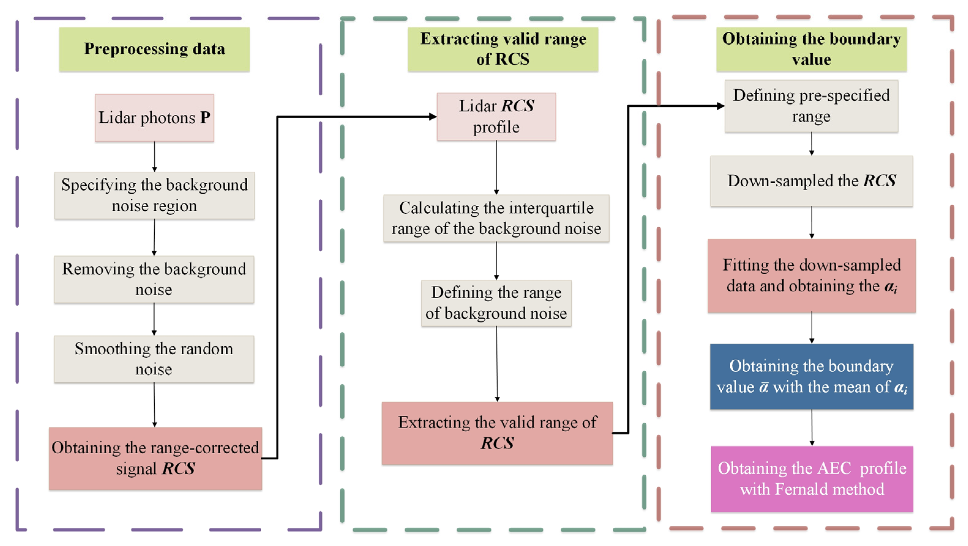
2.2. Extinction Coefficient Profile Inversion Algorithm

The Fernald backward algorithm is widely recognized as a stable method for retrieving extinction coefficients, and the key challenge lies in the estimation of the boundary value. The selection of the boundary position and its extinction coefficient estimation is crucial to determining the accuracy of the extinction coefficient profile for horizontal scanning lidar.

The proposed algorithm extracts the valid RCS, utilizing the low SNR RCS as the boundary at the far-end position. Extracting the valid RCS not only accelerates the convergence of the algorithm but also avoids the impact of error divergence caused by noise. Using the far end of the valid RCS as the boundary position can maximize the detection range, thus enhancing the detection capability of the lidar.

However, the SNR of the RCS at the far end is usually very low. The signal from atmospheric backscatter is mixed with noise and cannot be distinguished. An averaging approach is employed to reduce the disturbance from noise. The boundary value, representing the mean atmospheric extinction coefficient, is obtained and substituted into the Fernald backward algorithm to derive the extinction coefficient profile.

The proposed new algorithm is divided into the following three steps, and the flowchart is shown in Figure 1.

2.2.1. Preprocess the Data

The received lidar signals are not only from atmospheric backscatter but also include the background light and dark counts. A background noise correction is required. The last tens of range gates of the lidar signals are usually considered to be a noise-only region. The average of the signals in this region is taken as the noise $N_b$, which is then subtracted from the raw signal. Apart from the background noise, the lidar signal is also contaminated by a significant amount of random noise, which can be removed by applying a moving window smoothing technique.

As the laser propagates through the atmosphere, its energy decays with the distance, and the received backscattered signals are inversely proportional to the square of the distance. The lidar signals need to multiply the square of the distance to obtain the RCS.

2.2.2. Determine the Valid RCS

The background noise-corrected RCS indicates that the laser is subjected to atmospheric extinction during transmission. When the signal attenuates to the noise level, it becomes overwhelmed by noise and is considered invalid. Invalid signals cause errors when solving the lidar equation and should be discarded.

A valid RCS is defined as a continuous signal with an intensity above the noise level. The noise level depends on the last kilometer of the detected signal and is denoted as $RCS\left(r_{e-1},r_e\right)$. The interquartile range (IQR) principle is used to filter out noise signals $RCS\left(r_{e-1},r_e\right)$ The maximum noise level is defined as $\mu +2\epsilon$, with $\mu$ representing the mean and $\epsilon$ representing the standard deviation. The valid RCS is extracted as $RCS\left(r_0,r_v\right)$, where $r_0$ is the minimum range for complete lidar overlap and $r_v$ represents the maximum range where the RCS is greater than the noise.

2.2.3. Estimate the Boundary Extinction Coefficient

To maximize the detection range of lidar, we pre-specify the last two kilometers of the valid RCS as the boundary value estimation range. However, the last two kilometers of the valid RCS are affected by noise, resulting in significant errors in the fitted extinction coefficients. To improve the accuracy of the fitted extinction coefficient for low SNR signals, we perform multiple random down-sampling and averaging of the fitted extinction coefficients to reduce the impact of noise. The new down-sampled data are composed by randomly taking $m$ points from the original valid RCS, where $m$ is less than the total number of original RCS points. It should be noted that the range of the down-sampled data should be similar to the original RCS.

$n$ sets of down-sampled data are fitted separately to obtain the extinction coefficients ${\alpha }_i$, where the subscript $i$ represents the index of the down-sampled data.

The aerosol extinction coefficient (AEC) for each down-sampled datum is fitted separately. The fitting equation is expressed as

$$y=a\cdot \exp \left(b\cdot \Delta r\right)$$

(4)

where $y$ is the fitting signal of the low SNR range. The constant $a$ represents $C\left[{\displaystyle \frac{{\sigma }_1\left(r\right)}{S_1}}+{\displaystyle \frac{{\sigma }_2\left(r\right)}{S_2}}\right]$, and the constant $b$ represents $-2\left[{\sigma }_1\left(r^{\prime }\right)+{\sigma }_2\left(r^{\prime }\right)\right]$. The extinction coefficient of the molecule is obtained with the 1976 U.S. standard atmosphere model [41]. The down-sampled aerosol extinction coefficients ${\alpha }_i$ are obtained by

$${\alpha }_i=-0.5b-{\sigma }_1$$

(5)

As mentioned in Section 2.1, the extinction coefficient obtained from the low SNR RCS does not accurately represent the atmospheric extinction coefficient. We proposed averaging the extinction coefficients ${\alpha }_i$. The mean $\overline{\alpha }$ represents the aerosol extinction coefficient of the local atmosphere. Substitute $\overline{\alpha }$ as the boundary value into the Fernald backward solution to obtain the extinction coefficient profile [18].

The noise in lidar signals follows a Poisson distribution, as shown in Figure 2. The bootstrap method proved effective in mitigating the impact of the Poisson-distributed noise, thereby reducing the boundary value estimation errors for low SNR signals [42,43]. The variance of the error in the mean value is expressed as

$$\mathrm{Var}\left(\overline{\epsilon }\right)={\displaystyle \frac{1}{n^2}}{\displaystyle \sum _{i=1}^n\mathrm{Var}\left({\epsilon }_i\right)}={\displaystyle \frac{\mathrm{Var}\left({\epsilon }_i\right)}{n}}$$

(6)

where $n$ represents the number of samples, and ${\epsilon }_i$ represents the measurement error, which is independent and randomly distributed. The variance of the mean error decreases as the number of measurements $n$ increases. The computational efficiency is correlated with the number of fitting points: as the number of points increases, the efficiency of the down-sampling method improves significantly.

3. The Validation Experiments

3.1. Lidar Signal Simulation with Pre-Set Extinction Coefficient

We simulate a horizontal lidar signal to demonstrate the validation of the proposed algorithm in low SNR regions. The lidar backscattered signal is simulated based on the lidar Equation (1), assuming the lidar system constant of 2000 and a spatial resolution of 100 m. The horizontal extinction coefficient of atmospheric molecules is set to 0.013 km⁻¹ based on the 1976 U.S. standard atmosphere model [41]. The horizontal non-uniform extinction coefficient of atmospheric aerosol (blue line) is shown in Figure 3. The lidar ratios are set to $8\pi /3$ for atmospheric molecules and 20 for clean marine atmospheric aerosols [44]. The simulated lidar signal consists of the ideal signal combined with the Poisson-distributed noise (red line), as shown in Figure 3.

The simulated photon signals are preprocessed for denoising and range corrected in step 1, and the valid RCS is extracted as described in step 2 in Section 2. The simulated valid RCS is presented in Figure 4. The blue solid line represents the RCS and the black dashed line represents the noise level, with valid RCS signals lying above this threshold. The red solid line between the red vertical lines indicates the RCS signal used to calculate the boundary value.

3.2. The Result of the New Boundary Estimation Algorithm

As described in step 3 in Section 2, we randomly selected 10 sample points from the valid RCS within the pre-specified range to generate a set of down-sampled data. This process was repeated to obtain 20 different sets of down-sampled data. We only present 4 out of the 20 sets of down-sampled data, as shown in Figure 5. The line with circles represents the original RCS, while the line with stars represents the selected down-sampled data.

Each of the 20 sets of down-sampled data was fitted separately, resulting in 20 extinction coefficients. The range of the 20 down-sampled extinction coefficients was from 0.134 km⁻¹ to 0.170 km⁻¹. The mean of the down-sampled extinction coefficients was 0.152 km⁻¹, with a relative error of −23.9%. The extinction coefficient obtained by fitting the original RCS was 0.142 km⁻¹, with a relative error of −29.1%. The new algorithm achieved a 5.2% improvement in the accuracy of the extinction coefficient compared to the traditional method. To evaluate the method’s validity and robustness, we conducted 1000 Monte Carlo simulations with randomized signals. Figure 6 shows that the mean method produced more accurate boundary values in 794 cases (79.4% of the total simulations). Statistically, the accuracy of the mean method was 4.4% higher than that of the traditional overall method.

3.3. Error Analysis for the New Algorithm

For simplicity, we rewrite the Fernald backward method [18] as follows

$$\sigma \left(I-1\right)={\displaystyle \frac{1}{\frac{V_1\left(I\right)}{\sigma \left(I\right)}+V_2\left(I\right)}}$$

(7)

where $\sigma$ represents ${\sigma }_1\left(I-1\right)+{\displaystyle \frac{{\mathrm{S}}_1}{{\mathrm{S}}_2}}{\sigma }_2\left(I-1\right)$, $V_1$ represents ${\displaystyle \frac{X\left(I\right)}{X\left(I-1\right)\exp \left[A\left(I,I-1\right)\right]}}$ and $V_2$ represents $V_1\Delta R+\Delta R$. $X\left(I\right)$ represents the range-corrected signal $\mathrm{P}\left(r\right)r^2$ at the range bin $I$. $A$ represents the integral term for the backscatter coefficient of atmospheric molecules.

Assuming an error of $\Delta \sigma \left(I\right)$ at $I$, which propagates to $I-1$, the error becomes

$$\Delta \sigma \left(I-1\right)={\displaystyle \frac{\Delta \sigma \left(I\right)}{\left[V_1+V_2{\sigma }_e\left(I\right)\right]\left[1+\frac{V_2}{V_1}\sigma \left(I\right)\right]}}$$

(8)

where ${\sigma }_e\left(I\right)=\sigma \left(I\right)+\Delta \sigma \left(I\right)$, representing the estimated boundary value.

The propagation of the relative error of the extinction coefficients for the simulated signal is shown in Figure 7. The blue solid line represents the relative error of the boundary value based on the new algorithm, while the red solid line represents the relative error of the boundary value based on the direct fitting RCS. At the far end of the valid RCS, the relative error of the boundary value using the new algorithm is −23.8%, which is 5.2% more accurate than the direct fitting all-sample method (−29.3%).

It is noteworthy that, as the forward integration of the Fernald backward algorithm progresses, the relative error typically decreases. However, due to the low SNR of the simulated signal, the relative error fluctuates at the far end and only begins to stabilize at a distance of 4.19 km. This indicates that the RCS measurements are susceptible to noise interference that is difficult to eliminate, thereby introducing significant errors into the extinction coefficient retrieval. Reducing the boundary value estimation errors helps mitigate the noise-induced distortions along the lidar observation path, particularly in the far-end regions.

3.4. The Field Experiment

We further validated the performance of the mean method under low SNR conditions using real signals obtained from the horizontal scanning lidar at Shenzhen’s Marine Meteorological Observatory. The extinction coefficient measured by the coastal visibility sensors was used as the ground truth to evaluate the relative errors between the mean method (mean method) and the traditional method of fitting all the samples (all methods). It should be noted that due to the blind zone in the lidar’s near field, we utilized the average value from the 2–2.1 km range as the coastal extinction coefficient.

Figure 8a shows the RCS (blue line) measured at 22:52 on 10 April 2023, with the black dashed line representing the noise level and the red box indicating the RCS used for the boundary value calculation. The fitted valid signal (red line) yields an R² of 0.919, indicating that the atmosphere in this region is homogeneous.

Figure 8b compares the extinction coefficient profiles obtained through the mean method (blue solid line) and the all-sample method (red solid line). At the 11.16 km boundary position, the extinction coefficients derived from these methods are 0.25 km⁻¹ and 0.22 km⁻¹, respectively. When compared with the visibility sensor measurements, the relative errors are −1.7% for the mean method and −2.2% for the all-sample method, demonstrating their comparable accuracy under homogeneous conditions.

Figure 8c,d are similar to Figure 8a,b but correspond to an inhomogeneous atmosphere (R² = 0.011) at 09:54 on 11 April 2023. At the 10.05 km boundary position, the extinction coefficients from the two methods differ significantly, measuring 0.0195 km⁻¹ and 0.196 km⁻¹, respectively. The relative errors are −0.30% for the mean method versus −17.6% for the all-sample method, indicating a 17.3% improvement in accuracy achieved by the mean method under inhomogeneous atmospheric conditions.

4. Results

4.1. The Instrument and Observation

To verify the validity of the proposed algorithm, a series of continuous experiments were conducted from April 2023 to February 2024 at Shenzhen’s Marine Meteorological Observatory (22.48°N, 114.56°E). A scanning single-wavelength elastic lidar was employed to observe the horizontal optical properties of the aerosols. The lidar was installed 160 m away from the coast, allowing observation of the aerosols on the ocean surface. A photograph of the lidar is shown in Figure 9a, and the surrounding environment is shown in Figure 9b. A PWD forward scatter sensor was also installed in the observatory to provide visibility information.

The laser wavelength of the lidar was 1550 nm, which is in the near-infrared spectrum. The single pulse energy was 75 $\mathsf{\mu }\mathrm{J}$, which is eye-safe. The lidar’s spatial resolution was 30 m, with a maximum detection range of about 15 km.

To evaluate the performance of the proposed algorithm, we conducted a series of comparative experiments with the visibility observed by the forward scatter sensor in the observatory.

According to the Koschmieder’s law [45], the atmospheric visibility is obtained by

$$V={\displaystyle \frac{3.912}{{\sigma }_{550}}}$$

(9)

where ${\sigma }_{550}$ is the extinction coefficient of light of a wavelength of 550 nm. For other wavelength light, the visibility should be calibrated with

$$V_{\lambda }={\displaystyle \frac{3.912}{{\sigma }_{\lambda }}}{\left({\displaystyle \frac{\lambda }{550}}\right)}^{-q}$$

(10)

where $\lambda$ is 1550 nm for the employed lidar, ${\sigma }_{\lambda }$ is the extinction coefficient obtained by the 1550 nm lidar and the empirical value of $q$ is 1.3.

4.2. The Detection of Sea Fog

Shenzhen’s Marine Meteorological Observatory is located on the southern coast of China, which has a subtropical monsoon climate with abundant moisture. Spring is the peak season for sea fog along the coast of the South China Sea [46,47]. Coastal sea fog typically begins to form and develop during the night, dissipating early the next morning. Currently, most studies on the sea fog process are based on satellite images, which have low resolution and make it difficult to observe small-scale sea fog events. Lidar can finely and continuously observe the formation, development, and dissipation processes of small-scale sea fog [48,49,50].

We validated the performance of the proposed algorithm using a field experiment during a sea fog event from 10 to 11 April 2023. The spatial distribution of the extinction coefficients is shown in Figure 10a,f. The figure indicates that the detection range of the lidar was approximately 12 km before the occurrence of sea fog, and around 4 km at the peak of the fog. During the sea fog, the detection range of the lidar was significantly reduced. During the sea fog, the spatial distribution of the extinction coefficient was highly irregular. The boundary value estimation method based on the new algorithm can maximize the detection range of lidar within the effective RCS and is not constrained by atmospheric homogeneity. A visibility comparison experiment confirmed that the proposed mean algorithm demonstrated high accuracy in terms of visibility observation. As shown in Figure 11, during the sea fog, the PWD (blue line) and lidar (red line) results generally aligned, with the lidar measurements derived from the extinction coefficients averaged within 1–1.5 km offshore. The observed discrepancies around 01:00, 03:00 and 07:30 (green dashed rectangles) were attributed to the lidar’s near-field blind zone (requiring extinction coefficients ~1 km offshore) and spatial variability caused by the atmospheric heterogeneity between measurement locations.

5. Conclusions

The inversion of the atmospheric extinction coefficient profiles based on lidar data usually relies on a priori boundary values. These boundary values are often determined by fitting based on uniform regions of the atmosphere. In the atmosphere, low SNR signals are disturbed by noise and are easily misclassified as inhomogeneous regions. The boundary values determined by directly fitting such signals will introduce large errors. Therefore, these low SNR signals are typically excluded from the boundary value fitting process. Although this method can effectively improve the accuracy of the boundary value, it also reduces the effective detection range of the lidar.

To overcome this challenge, this paper proposes a new method: by performing multiple random samplings, a down-sampled low SNR RCS dataset is constructed, and the boundary values are determined using the averaged fitting results of these datasets, thereby reducing the impact of noise on the outcome. Simulation experiments show that, compared to the method of directly fitting the low SNR RCS, the new algorithm reduces the relative error of the boundary value estimation by approximately 5%, demonstrating higher accuracy in low SNR environments. Two distinct measured atmospheric RCS are employed to validate the proposed algorithm. The proposed algorithm maintains consistent accuracy when processing high R² signals that characterize homogeneous atmospheric conditions with high SNR. The proposed algorithm demonstrates enhanced performance when processing low R² signals that characterize low SNR signals or in inhomogeneous conditions, achieving a 17.3% accuracy improvement compared to the traditional method.

In addition, we applied the algorithm to horizontally scanned signals and successfully generated the temporal variation of the visibilities and a two-dimensional distribution map of the AEC during the sea fog event. This result helps to comprehensively capture the development of sea fog and provides important information for a deeper understanding of its physical evolution.

References

1. Li, Z.; Lau, W.M.; Ramanathan, V.; Wu, G.; Ding, Y.; Manoj, M.G.; Liu, J.; Qian, Y.; Li, J.; Zhou, T.; et al. Aerosol and Monsoon Climate Interactions over Asia. Rev. Geophys. 2016, 54, 866–929. [Google Scholar] [CrossRef]
2. Guo, J.; Deng, M.; Lee, S.S.; Wang, F.; Li, Z.; Zhai, P.; Liu, H.; Lv, W.; Yao, W.; Li, X. Delaying Precipitation and Lightning by Air Pollution over the Pearl River Delta. Part I: Observational Analyses. J. Geophys. Res. Atmos. 2016, 121, 6472–6488. [Google Scholar] [CrossRef]
3. Molnár, A.; Imre, K.; Ferenczi, Z.; Kiss, G.; Gelencsér, A. Aerosol Hygroscopicity: Hygroscopic Growth Proxy Based on Visibility for Low-Cost PM Monitoring. Atmos. Res. 2020, 236, 104815. [Google Scholar] [CrossRef]
4. Li, J.; Carlson, B.E.; Yung, Y.L.; Lv, D.; Hansen, J.; Penner, J.E.; Liao, H.; Ramaswamy, V.; Kahn, R.A.; Zhang, P.; et al. Scattering and Absorbing Aerosols in the Climate System. Nat. Rev. Earth Environ. 2022, 3, 363–379. [Google Scholar] [CrossRef]
5. Ansmann, A.; Müller, D. Lidar and Atmospheric Aerosol Particles. In Lidar; Weitkamp, C., Ed.; Springer Series in Optical Sciences; Springer: New York, NY, USA, 2005; Volume 102, pp. 105–141. ISBN 978-0-387-40075-4. [Google Scholar]
6. Amiridis, V.; Balis, D.S.; Kazadzis, S.; Bais, A.; Giannakaki, E.; Papayannis, A.; Zerefos, C. Four-year Aerosol Observations with a Raman Lidar at Thessaloniki, Greece, in the Framework of European Aerosol Research Lidar Network (EARLINET). J. Geophys. Res. Atmos. 2005, 110, D21203. [Google Scholar] [CrossRef]
7. Baars, H.; Ansmann, A.; Althausen, D.; Engelmann, R.; Heese, B.; Müller, D.; Artaxo, P.; Paixao, M.; Pauliquevis, T.; Souza, R. Aerosol Profiling with Lidar in the Amazon Basin during the Wet and Dry Season. J. Geophys. Res. Atmos. 2012, 117, D21201. [Google Scholar] [CrossRef]
8. Lin, C.Q.; Li, C.C.; Lau, A.K.H.; Yuan, Z.B.; Lu, X.C.; Tse, K.T.; Fung, J.C.H.; Li, Y.; Yao, T.; Su, L.; et al. Assessment of Satellite-Based Aerosol Optical Depth Using Continuous Lidar Observation. Atmos. Environ. 2016, 140, 273–282. [Google Scholar] [CrossRef]
9. Ma, X.; Wang, C.; Han, G.; Ma, Y.; Li, S.; Gong, W.; Chen, J. Regional Atmospheric Aerosol Pollution Detection Based on LiDAR Remote Sensing. Remote Sens. 2019, 11, 2339. [Google Scholar] [CrossRef]
10. Yin, Z.; Yi, F.; Liu, F.; He, Y.; Zhang, Y.; Yu, C.; Zhang, Y. Long-Term Variations of Aerosol Optical Properties over Wuhan with Polarization Lidar. Atmos. Environ. 2021, 259, 118508. [Google Scholar] [CrossRef]
11. Vernier, J.P.; Pommereau, J.P.; Garnier, A.; Pelon, J.; Larsen, N.; Nielsen, J.; Christensen, T.; Cairo, F.; Thomason, L.W.; Leblanc, T.; et al. Tropical Stratospheric Aerosol Layer from CALIPSO Lidar Observations. J. Geophys. Res. 2009, 114, D00H10. [Google Scholar] [CrossRef]
12. Liu, Z.; Omar, A.; Vaughan, M.A.; Hair, J.; Kittaka, C.; Hu, Y.; Powell, K.; Trepte, C.; Winker, D.; Hostetler, C.; et al. CALIPSO Lidar Observations of the Optical Properties of Saharan Dust: A Case Study of Long-range Transport. J. Geophys. Res. Atmos. 2008, 113, D07207. [Google Scholar] [CrossRef]
13. Varnai, T.; Marshak, A. Global CALIPSO Observations of Aerosol Changes Near Clouds. IEEE Geosci. Remote Sens. Lett. 2011, 8, 19–23. [Google Scholar] [CrossRef]
14. Solomon, S.; Daniel, J.S.; Neely, R.R.; Vernier, J.-P.; Dutton, E.G.; Thomason, L.W. The Persistently Variable “Background” Stratospheric Aerosol Layer and Global Climate Change. Science 2011, 333, 866–870. [Google Scholar] [CrossRef] [PubMed]
15. Kremser, S.; Thomason, L.W.; Von Hobe, M.; Hermann, M.; Deshler, T.; Timmreck, C.; Toohey, M.; Stenke, A.; Schwarz, J.P.; Weigel, R.; et al. Stratospheric Aerosol-Observations, Processes, and Impact on Climate: Stratospheric Aerosol. Rev. Geophys. 2016, 54, 278–335. [Google Scholar] [CrossRef]
16. Jia, R.; Liu, Y.; Hua, S.; Zhu, Q.; Shao, T. Estimation of the Aerosol Radiative Effect over the Tibetan Plateau Based on the Latest CALIPSO Product. J. Meteorol. Res. 2018, 32, 707–722. [Google Scholar] [CrossRef]
17. Fernald, F.G.; Herman, B.M.; Reagan, J.A. Determination of Aerosol Height Distributions by Lidar. J. Appl. Meteorol. 1972, 11, 482–489. [Google Scholar] [CrossRef]
18. Fernald, F.G. Analysis of Atmospheric Lidar Observations: Some Comments. Appl. Opt. 1984, 23, 652–653. [Google Scholar] [CrossRef]
19. Klett, J.D. Stable Analytical Inversion Solution for Processing Lidar Returns. Appl. Opt. 1981, 20, 211. [Google Scholar] [CrossRef]
20. Sasano, Y.; Nakane, H. Significance of the Extinction/Backscatter Ratio and the Boundary Value Term in the Solution for the Two-Component Lidar Equation. Appl. Opt. 1984, 23, 11_1–13. [Google Scholar] [CrossRef]
21. Rocadenbosch, F.; Reba, M.N.M.D.; Sicard, M.; Comerón, A. Practical Analytical Backscatter Error Bars for Elastic One-Component Lidar Inversion Algorithm. Appl. Opt. 2010, 49, 3380–3393. [Google Scholar] [CrossRef]
22. Qiu, J. Sensitivity of Lidar Equation Solution to Boundary Values and Determination of the Values. Adv. Atmos. Sci. 1988, 5, 229–241. [Google Scholar] [CrossRef]
23. Matsumoto, M.; Takeuchi, N. Effects of Misestimated Far-End Boundary Values on Two Common Lidar Inversion Solutions. Appl. Opt. 1994, 33, 6451–6456. [Google Scholar] [CrossRef] [PubMed]
24. Cao, N.; Yang, F.; Zhu, C. Improving the Accuracy of Aerosol Extinction Coefficient Inversion. Opt. Spectrosc. 2014, 116, 649–653. [Google Scholar] [CrossRef]
25. Ong, P.M.; Lagrosas, N.; Shiina, T.; Kuze, H. Surface Aerosol Properties Studied Using a Near-Horizontal Lidar. Atmosphere 2019, 11, 36. [Google Scholar] [CrossRef]
26. Liu, H.; Mao, M. An Accurate Inversion Method of Aerosol Extinction Coefficient about Ground-Based Lidar without Needing Calibration. Acta Phys. Sin. 2019, 68, 074205. [Google Scholar] [CrossRef]
27. Sun, G.; Qin, L.; Zhang, S.; He, F.; Tan, F.; Jing, X.; Hou, Z. A New Method of Measuring Boundary Value of Atmospheric Extinction Coefficient. Acta Phys. Sin. 2018, 67, 054205. [Google Scholar] [CrossRef]
28. Ma, Y.; Liu, J.; Chen, N.; Gao, H.; Xiong, X. Determination of the Boundary Value of the Aerosol Extinction Coefficient and Its Effects on the Extinction Coefficient Profile of Aerosol in Lower Atmosphere. Optik 2018, 160, 283–297. [Google Scholar] [CrossRef]
29. Li, H.; Chang, J.; Xu, F.; Liu, B.; Liu, Z.; Zhu, L.; Yang, Z. An RBF Neural Network Approach for Retrieving Atmospheric Extinction Coefficients Based on Lidar Measurements. Appl. Phys. B 2018, 124, 184. [Google Scholar] [CrossRef]
30. Ferguson, J.A.; Stephens, D.H. Algorithm for Inverting Lidar Returns. Appl. Opt. 1983, 22, 3673–3675. [Google Scholar] [CrossRef]
31. Xian, J.; Han, Y.; Huang, S.; Sun, D.; Zheng, J.; Han, F.; Zhou, A.; Yang, S.; Xu, W.; Song, Q.; et al. Novel Lidar Algorithm for Horizontal Visibility Measurement and Sea Fog Monitoring. Opt. Express 2018, 26, 34853–34863. [Google Scholar] [CrossRef]
32. Xian, J.; Sun, D.; Xu, W.; Han, Y.; Zheng, J.; Peng, J.; Yang, S. Urban Air Pollution Monitoring Using Scanning Lidar. Environ. Pollut. 2020, 258, 113696. [Google Scholar] [CrossRef] [PubMed]
33. Collis, R.T.H. Lidar: A New Atmospheric Probe. Q. J. R. Meteorol. Soc. 1966, 92, 220–230. [Google Scholar] [CrossRef]
34. Shang, X.; Xia, H.; Dou, X.; Shangguan, M.; Li, M.; Wang, C. Adaptive Inversion Algorithm for 1.5 μm Visibility Lidar Incorporating in Situ Angstrom Wavelength Exponent. Opt. Commun. 2018, 418, 129–134. [Google Scholar] [CrossRef]
35. Rocadenbosch, F.; Comerón, A.; Albiol, L. Statistics of the Slope-Method Estimator. Appl. Opt. 2000, 39, 6049–6057. [Google Scholar] [CrossRef]
36. Kunz, G.J.; De Leeuw, G. Inversion of Lidar Signals with the Slope Method. Appl. Opt. 1993, 32, 3249–3256. [Google Scholar] [CrossRef]
37. Mao, F.; Wang, W.; Min, Q.; Gong, W. Approach for Selecting Boundary Value to Retrieve Mie-Scattering Lidar Data Based on Segmentation and Two-Component Fitting Methods. Opt. Express 2015, 23, A604–A613. [Google Scholar] [CrossRef] [PubMed]
38. Mao, F.; Li, J.; Li, C.; Gong, W.; Min, Q.; Wang, W. Nonlinear Physical Segmentation Algorithm for Determining the Layer Boundary from Lidar Signal. Opt. Express 2015, 23, A1589–A1602. [Google Scholar] [CrossRef]
39. Zeng, X.; Xia, M.; Ge, Y.; Guo, W.; Yang, K. On-Site Ocean Horizontal Aerosol Extinction Coefficient Inversion under Different Weather Conditions on the Bo-Hai and Huang-Hai Seas. Atmos. Environ. 2018, 177, 18–27. [Google Scholar] [CrossRef]
40. Fei, R.; Kong, Z.; Wang, X.; Zhang, B.; Gong, Z.; Liu, K.; Hua, D.; Mei, L. Retrieval of the Aerosol Extinction Coefficient from Scanning Scheimpflug Lidar Measurements for Atmospheric Pollution Monitoring. Atmos. Environ. 2023, 309, 119945. [Google Scholar] [CrossRef]
41. Krueger, A.J.; Minzner, R.A. A Mid-Latitude Ozone Model for the 1976 US Standard Atmosphere. J. Geophys. Res. 1976, 81, 4477–4481. [Google Scholar] [CrossRef]
42. Efron, B. Bootstrap Methods: Another Look at the Jackknife. Ann. Stat. 1979, 7, 1–26. [Google Scholar] [CrossRef]
43. Zhu, F.; Qin, B.; Feng, W.; Wang, H.; Huang, S.; Lv, Y.; Chen, Y. Reducing Poisson Noise and Baseline Drift in X-Ray Spectral Images with Bootstrap Poisson Regression and Robust Nonparametric Regression. Phys. Med. Biol. 2013, 58, 1739–1758. [Google Scholar] [CrossRef]
44. Doherty, S.J.; Anderson, T.L.; Charlson, R.J. Measurement of the Lidar Ratio for Atmospheric Aerosols with a 180° Backscatter Nephelometer. Appl. Opt. 1999, 38, 1823–1832. [Google Scholar] [CrossRef] [PubMed]
45. Janeiro, F.M.; Wagner, F.; Ramos, P.M.; Silva, A.M. Atmospheric Visibility Measurements Based on a Low-Cost Digital Camera. In Proceedings of the ConfTele, 6th Conference on Telecommunications, Peniche, Portugal, 9–11 May 2007; pp. 213–216. [Google Scholar]
46. Huang, H.; Liu, H.; Jiang, W.; Huang, J.; Mao, W. Characteristics of the Boundary Layer Structure of Sea Fog on the Coast of Southern China. Adv. Atmos. Sci. 2011, 28, 1377–1389. [Google Scholar] [CrossRef]
47. Huang, H.; Huang, B.; Yi, L.; Liu, C.; Tu, J.; Wen, G.; Mao, W. Evaluation of the Global and Regional Assimilation and Prediction System for Predicting Sea Fog over the South China Sea. Adv. Atmos. Sci. 2019, 36, 623–642. [Google Scholar] [CrossRef]
48. Xu, W.; Yang, H.; Sun, D.; Qi, X.; Xian, J. Lidar System with a Fast Scanning Speed for Sea Fog Detection. Opt. Express 2022, 30, 27462–27471. [Google Scholar] [CrossRef]
49. Xiao, Y.; Liu, R.; Ma, Y.; Cui, T. MERRA-2 Reanalysis-Aided Sea Fog Detection Based on CALIOP Observation over North Pacific. Remote Sens. Environ. 2023, 292, 113583. [Google Scholar] [CrossRef]
50. Zhu, J.; Chen, Y.; Zhang, L.; Jia, X.; Feng, Z.; Wu, G.; Yan, X.; Zhai, J.; Wu, Y.; Chen, Q.; et al. Demonstration of Measuring Sea Fog with an SNSPD-Based Lidar System. Sci. Rep. 2017, 7, 15113. [Google Scholar] [CrossRef]
Figure 1. The flowchart of the new algorithm.
Remotesensing 17 01736 g001
Figure 2. Lidar photon noise following a Poisson distribution.
Remotesensing 17 01736 g002
Figure 3. The simulated aerosol extinction coefficient (blue line) and lidar signal (red line).
Remotesensing 17 01736 g003
Figure 4. The simulated RCS and the range for the boundary value estimation.
Remotesensing 17 01736 g004
Figure 5. Original data and down-sampled data.
Remotesensing 17 01736 g005
Figure 6. Statistical results of the simulation signals.
Remotesensing 17 01736 g006
Figure 7. The relative errors of the extinction coefficient profiles from the Fernald method with the boundary value obtained from the new algorithm (blue solid line) and all-sample fitted method (red solid line).
Remotesensing 17 01736 g007
Figure 8. (a) Homogeneous atmospheric RCS measured on 10 April 2023 (22:52), (b) extinction coefficient profiles derived from the RCS of (a,c) the inhomogeneous atmospheric RCS measured on 11 April 2023 (09:54) and (d) extinction coefficient profiles derived from the RCS of (c).
Remotesensing 17 01736 g008aRemotesensing 17 01736 g008b
Figure 9. Photograph of the lidar (a) and the location (b).
Remotesensing 17 01736 g009
Figure 10. The spatial distribution of the extinction coefficient at (a) 23:45 on 10 April and (b) 01:21, (c) 01:37, (d) 04:13, (e) 04:45, and (f) 07:02 on 11 April.
Remotesensing 17 01736 g010
Figure 11. The temporal variation of the visibility from the evening of 10 April to the morning of 11 April 2023, showing a discrepancy between lidar and PWD observations within the green dash boxes.
Remotesensing 17 01736 g011
Disclaimer/Publisher’s Note: The statements, opinions and data contained in all publications are solely those of the individual author(s) and contributor(s) and not of MDPI and/or the editor(s). MDPI and/or the editor(s) disclaim responsibility for any injury to people or property resulting from any ideas, methods, instructions or products referred to in the content.