Abstract
In recent years, great progress has been made in the field of super-resolution (SR) reconstruction based on deep learning techniques. Although image SR techniques show strong potential in image reconstruction, the effective application of these techniques to SR reconstruction of digital elevation models (DEMs) remains an important research challenge. The complexity and diversity of DEMs limits existing methods to capture subtle changes and features of the terrain, thus affecting the quality of reconstruction. To solve this problem, a DEM SR reconstruction network based on multi-path feature extraction and transformer feature enhancement is proposed in this paper. The network structure has three parts: feature extraction, image reconstruction, and feature enhancement. The feature extraction component consists of three feature extraction blocks, and each feature extraction block contains multiple multi-path feature residuals to enhance the interaction between spatial information and semantic information, so as to fully extract image features. In addition, the transformer feature enhancement module uses an encoder and decoder based design, leveraging the correlation between low- and high-dimensional features to further improve network performance. Through repeated testing and improvement, the model shows excellent performance in high-resolution DEM image reconstruction, and can generate more accurate DEMs. In terms of elevation and slope evaluation indexes, the model was 3.41% and 1.11% better compared with the existing reconstruction methods, which promotes the application of SR reconstruction technology in terrain data.
1. Introduction
Digital elevation models (DEMs) are crucial data formats in geographic information systems for representing variations in the Earth’s surface elevation. DEMs are widely used across various fields [1], including urban planning, environmental monitoring, soil erosion assessment, disaster management, and transportation network analysis, providing essential topographical information for researchers and decision-makers [2]. By accurately depicting surface undulations, DEMs facilitate a deeper understanding and simulation of natural environments. However, traditional DEMs often face limitations in spatial resolution, particularly in applications requiring high detail, such as urban modeling and ecosystem studies. Low-resolution (LR) DEMs struggle to meet analytical demands in these contexts [3]. Therefore, super-resolution (SR) reconstruction of DEMs becomes particularly necessary, as increasing the spatial resolution of DEMs allows better capture of terrain details, supporting more precise analysis and decision-making, thereby enhancing the effectiveness and accuracy of various applications.
Image SR reconstruction is a significant technique in the field of image processing, aimed at recovering high-resolution (HR) images from LR inputs [4]. Image SR methods can be classified into three categories based on reconstruction strategies: interpolation-based, reconstruction-based, and learning-based methods. Interpolation-based methods enhance image resolution by estimating the pixel values of target pixels using the grayscale values of neighboring pixels. While simple to implement, these methods are prone to artifacts such as jagged edges and image blurring, making them inadequate for high-precision requirements. Conversely, reconstruction-based methods build an image degradation model that constrains the generation process of HR images using prior knowledge. Although these methods maintain edges and detailed information better, they involve significant computational complexity and a strong dependence on prior knowledge.
In recent years, learning-based approaches, particularly those utilizing deep learning, have made remarkable progress in SR reconstruction. These methods leverage large-scale HR image datasets to train models that learn the complex mapping between LR and HR images, enabling the generation of more realistic and nuanced HR images during reconstruction [5]. Despite the impressive potential of image SR technology in image reconstruction, effectively translating and applying these techniques to the SR reconstruction of terrain data remains a pressing research challenge. When it comes to SR reconstruction of DEM data, existing SR reconstruction methods face some challenges and limitations. Compared with ordinary image data, terrain data has unique properties. Terrain features typically exhibit complex topological structures and spatial distributions. For example, mountains, valleys, and plateaus have different geometric shapes and elevation gradients. The existing methods mainly developed for general images may not accurately capture these specific topological features of the terrain. They may oversimplify the complex elevation changes in DEM data, resulting in the loss of important terrain information. Accurate representation of subtle changes and features is crucial in high-resolution applications of DEM data. However, existing SR reconstruction methods often produce suboptimal results when applied to terrain data. They often fail to capture some elevation fluctuations, and these details are crucial for applications such as hydrological modeling, urban planning, and ecological research. Given the inherent complexity and diversity of terrain data, existing SR reconstruction methods often produce suboptimal results when applied to terrain data, often failing to capture key subtle changes and features in HR applications. Therefore, developing efficient and accurate SR reconstruction algorithms suitable for terrain data requirements has become a focus of contemporary research. Consequently, the development of efficient and accurate SR reconstruction algorithms tailored to the needs of terrain data has become a focal point of contemporary research.
In this paper, a DEM SR reconstruction network based on a convolutional neural network (CNN) architecture is proposed. The multi-path feature extraction module (MPFEM) and transformer feature enhancement module are mainly used. MPFEM focuses on the detailed extraction and interactive enhancement of spatial and semantic information to obtain rich basic features, including the multipath residual blocks (MPRBs) we designed. The transformer feature enhancement module can further process the basic features output by the multi-path feature extraction module, promoting the deep fusion of high-dimensional features and low-dimensional features. Through experiments, we have found the appropriate number of layers of encoders and decoders. The combination of the two enables the network to not only fully explore local detail features but also integrate and optimize the features from a global perspective, achieving complementary advantages at the feature level. The main contributions of this study are as follows:
- An SR reconstruction network of DEMs based on multi-path feature extraction and transformer feature enhancement is proposed. Experiments show that this method is superior to the existing SR method and can reconstruct HR DEM with higher accuracy.
- A multipath feature extraction module (MPFEM) is proposed, which contains multi-path residual blocks (MPRBs), and utilizes multipath extraction, an extended convolution layer and a shuffle attention (SA) layer to enhance the interactivity between spatial information and semantic information.
- A transformer-based feature enhancement module is proposed, which is composed of multiple encoders and decoders, and processes the output of each feature extraction module, thus promoting the blending of high-dimensional features and low-dimensional features and improving network performance.
2. Related Work
2.1. Image SR Reconstruction Based on CNNs
The application of CNNs in the field of image SR has sparked extensive research and achieved significant progress. CNN-based methods leverage convolutional and pooling layers to extract features from LR images and progressively map them to HR images [6]. In 2014, Dong et al., first introduced CNNs into the realm of image SR, proposing a straightforward SR reconstruction method known as SRCNN [7]. This network consists of three layers, each with varying kernel sizes and filter counts, which enhances the capability for feature extraction. Additionally, the inclusion of nonlinear mapping functions after each convolutional layer further improves the network’s nonlinear expressive power. Compared to traditional image SR techniques, the images generated by SRCNN exhibit superior visual perception. However, due to the limited number of layers and the relatively large convolutional kernels, SRCNN faces challenges in extracting deep features, which may result in the loss of some details during image reconstruction.In 2016, Chao et al. proposed a fast SR reconstruction method called FSRCNN [8], which is based on CNNs and utilizes smaller convolutional kernels to simplify the network structure while employing small filters to reduce computational complexity. FSRCNN transforms LR images into HR images through convolutional and deconvolutional layers [9], achieving higher evaluation scores and improved image reconstruction results. In the same year, Kim et al., enhanced feature extraction by increasing the model’s depth and introduced the deep recursive convolutional network (DRCN) [10]. This method employs skip connections and recursive supervision to enhance training stability and improve the quality of the reconstructed images. In 2017, Lim et al., proposed the enhanced deep residual network (EDSR) [11], building upon the concepts of CNNs and residual networks (ResNet) [12] and applying them to image SR reconstruction. In EDSR, the researchers opted to remove the batch normalization (BN) layers to free up computational resources, allowing for the addition of more network layers under the same resource constraints, thereby enhancing the feature extraction capability of each layer.
2.2. DEM SR Reconstruction
SR reconstruction of DEMs is an important research direction in the field of geographic information science. In recent years, driven by the rapid development of deep learning technology, more and more research has been done in this field. Different from remote sensing image SR reconstruction, remote sensing image SR reconstruction aims to improve image resolution and make ground objects clearer for ground object identification, urban planning, etc. While taking pixel value, structure texture and visual effect into account for evaluation, DEM super-resolution reconstruction aims at terrain elevation data and improves resolution by specific methods to more accurately present terrain details. Used in geology, hydrology, and other fields, the evaluation focuses on the accuracy of elevation values and topographic parameters. In 2015, Xu et al., proposed a non-local algorithm (D-SRCNN) [13], which partitions DEMs into different categories of patches based on their correlation with HR images and recovers high-quality HR DEMs by training on similar patches, demonstrating superior performance compared to other non-local methods. In the same year, Xu et al., also introduced a CNN-based SR reconstruction model known as the enhanced deep SR network (EDSR) [14]. This method pre-trains the network using natural images to learn the relationship between LR and HR features in natural images, followed by fine-tuning the model with DEM data to better adapt to the reconstruction tasks of terrain data. Additionally, Yu et al., designed a regularization framework that integrates multiple data sources into the corresponding DEM, generating HR DEM data with broader coverage [15]. This approach excels in handling complex terrain features, noise, and data voids. In 2018, Argudo et al. proposed a fully CNN that utilizes LR DEMs and their HR orthophotos for SR reconstruction [16], achieving favorable results. In 2020, Xia et al., improved the efficient sub-pixel CNN (ESPCN) by introducing the recursive sub-pixel convolutional network (RSPCN) [17]. This method incorporated an “adding-zero” boundary handling technique to enhance the accuracy and convergence of RSPCN, resulting in better reconstruction outcomes. In 2021, Zhou et al., proposed an enhanced dual-filter deep residual neural network (EDEM-SR) [18], which enhances network performance by introducing residual structures and filters with different receptive fields, thereby improving the model’s ability to capture DEM features and reconstruct more realistic HR DEMs. In 2022, Lin et al., [19] employed an internal learning method to learn the internal priors of DEMs, generating an LR DEM dataset rich in image features and subsequently constructing a training framework to constrain external learning networks, yielding superior SR reconstruction results. In 2023, Han et al., proposed a DEM deep learning network based on global information constraints [20], which enhanced the effect of terrain data reconstruction through the use of a global information supplement module and a local feature generation module. In 2024, Yao et al., developed a new continuous representation model [21], which obtains height values at arbitrary query locations through encoder–decoder networks for learning from discrete elevation data in DEM super-resolution tasks.
2.3. Multi-Scale Feature Extraction and Fusion Module
Scale feature extraction and fusion are crucial techniques in computer vision and image processing. Their primary objective is to extract and fuse image features from various scales to enhance the accuracy and robustness of recognition and understanding [22]. This methodology can be categorized into three types: image pyramid methods [23], scale-space methods [24], and deep learning approaches [25].The image pyramid method generates images of different resolutions by scaling, thereby extracting features at each scale and capturing detailed information across various scales. The scale-space method constructs a scale space using techniques such as Gaussian filtering to extract features at different scales, reflecting the image information across these scales. The deep learning approach utilizes deep learning models to automatically learn multi-scale features by stacking convolutional layers and pooling layers, progressively extracting features from lower to higher levels, encompassing different scales and degrees of abstraction.
Extensive research indicates that effectively leveraging the rich scale information contained in LR images is vital for reconstructing high-quality images. Many researchers have adopted multi-scale feature extraction and fusion techniques to enhance network performance. In 2018, Li et al. [26] were the first to introduce a multi-scale strategy in SR tasks, which was realized by employing convolutional kernels of varying sizes and increasing the number of channels. They also proposed a multi-scale dense cross module to improve information transfer between convolutional layers. However, these methods face limitations due to the restricted receptive fields of their convolutional kernels, which do not effectively balance the relationship between the number of parameters and performance. By combining multi-path learning with feature fusion, SR models can better extract image features from multiple scales. For instance, Qin et al. [27] and Zhang et al. [28] proposed various multi-path structures and employed a hierarchical feature fusion structure (HFFS) to integrate global features. Nonetheless, these methods are limited to two paths, constraining their feature extraction capabilities, and HFFS introduces significant computational burdens. In 2021, Feng et al. [29] designed multi-scale fractal residual modules and multi-path structures that can effectively extract multi-scale features; In 2022, Lv et al. [30] extracted features from different layers using a multi-scale dense fusion module.
2.4. Application of Transformers in SR Reconstruction
In recent years, the transformer architecture has achieved remarkable success across various fields, particularly in natural language processing and computer vision. Its primary advantage lies in the self-attention mechanism, which effectively captures long-distance dependencies within input data, thereby enhancing model performance.
In the context of image SR reconstruction, transformers are extensively employed for feature extraction and information integration. In 2020, Yang et al. [31] proposed a texture-based SR reconstruction method that utilizes a transformer model to model the texture features present in images. This model consists of a learnable texture extractor, a correlation embedding module, a hard attention module, and a soft attention module. By stacking multiple texture transformer modules, the model is capable of recovering texture information from various scales, thereby improving the effectiveness of SR reconstruction. In 2021, Lu et al. [32] introduced a lightweight transformer model designed to achieve high-quality image SR reconstruction with reduced computational overhead. This model incorporates an efficient multi-head attention (EMHA) mechanism, which partitions large-scale matrix multiplications into smaller-scale operations, thus alleviating the computational burden. In the same year, Liu et al. [33] proposed a window-based transformer model known as the Swin transformer, which decreases computational complexity by segmenting images into patches and performing self-attention calculations within these windows. Liang et al. [34] applied this model to the task of image SR reconstruction, achieving favorable reconstruction results. This method learns residual information and adds it to the LR images prior to upsampling, effectively addressing the issue of information isolation between image patches through a window partitioning strategy. This approach enhances the model’s generalization capability, resulting in high-quality image reconstruction.
3. Method
3.1. Network Architecture
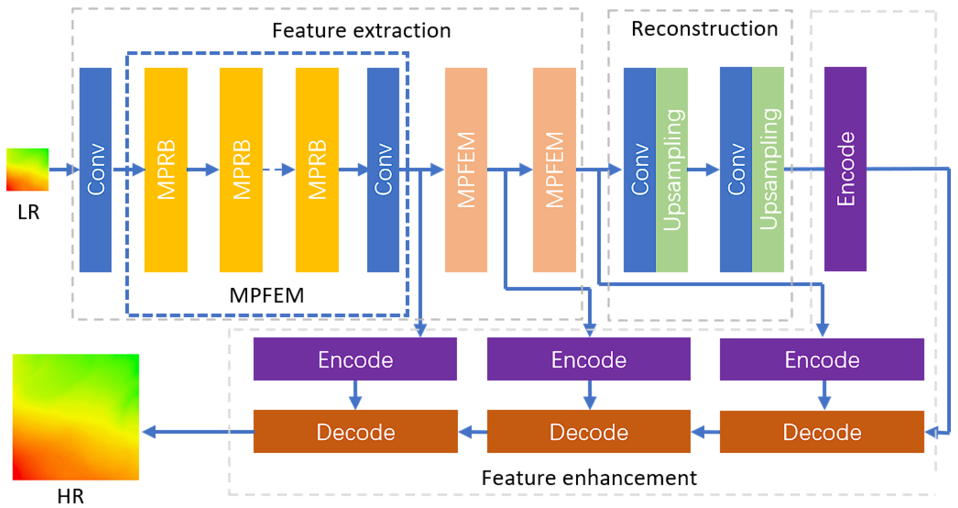
Based on a CNN architecture, this study proposes an MPFEM and a transformer feature enhancement module specifically designed for the SR reconstruction of DEMs, as illustrated in Figure 1. The MPFEM employs a multi-path network and SA layers, effectively extracting low-dimensional features from the DEM. The transformer feature enhancement module leverages the low-dimensional features prior to the upsampling layer and the high-dimensional features obtained from the upsampling layer, thereby further improving the accuracy of the reconstructed DEM. The network architecture is shown in Figure 1.

Figure 1.
Network architecture.
In the DEM SR reconstruction network, the LR feature image is initially processed through a convolutional layer to extract shallow features. This process can be mathematically represented as follows:
In (1), represents the shallow features extracted by the first convolutional layer, denotes the feature image of the LR DEM, and signifies the mapping relationship of the first convolutional layer.
After the extraction of shallow features, the feature image sequentially passes through three MPFEMs, which utilize a multi-path network architecture to extract and fuse network features of varying depths. The process through the MPRB is outlined as follows:
In (2)–(4), denotes the output features from the i-th MPFEM, while represents the feature mapping relationship of the i-th module.
Following the output from the three MPFEMs, the feature image proceeds to the upsampling layer for image magnification. This process can be mathematically expressed as:
In (5) and (6), denotes the feature image output after passing through the convolutional layer, and represents the output generated by the upsampling layer. The function indicates the feature mapping relationship of the upsampling layer. In the model designed for fourfold magnification, two such structures are employed. After the upsampling operation, the output is fed into the transformer feature enhancement module, which consists of three layers of encoders and decoders.
3.1.1. Multi-Path Feature Extraction Module
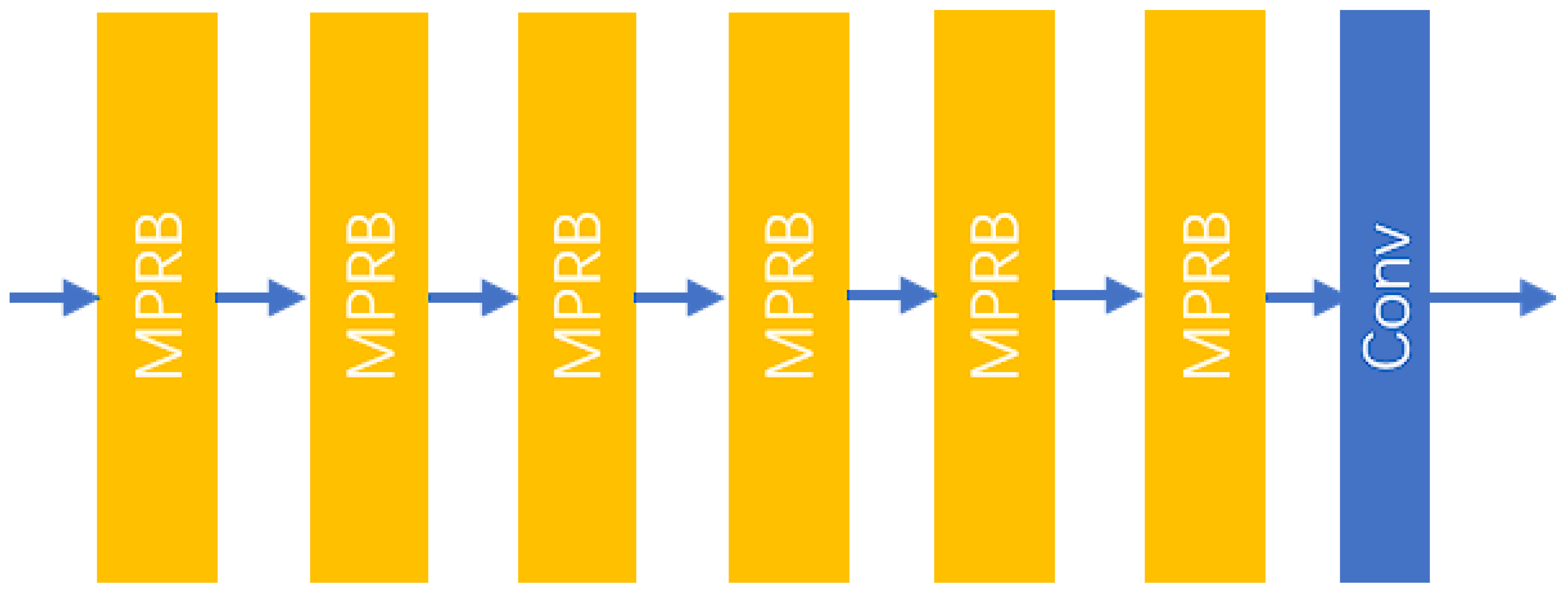
SR is a pixel-level task, and previous works have often focused on constructing deep network architectures along a single path. However, the network requires effective multi-scale feature representations to accurately predict detailed information. Furthermore, the width of the network is as crucial as its depth; neural networks with rectified linear unit (ReLU) activation functions need sufficient width to maintain their general approximation properties as depth increases. Therefore, this study shifts the focus from previously deeper and narrower architectures to deeper and wider architectures. To adequately extract the rich scale information present in LR images, this research designs an MPFEM. This module consists of several MPRBs and a convolutional layer, as illustrated in Figure 2.
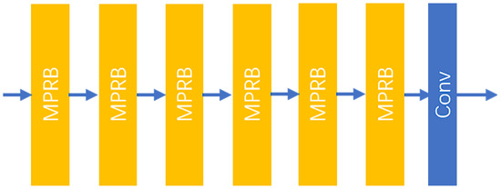
Figure 2.
The structure of the MPFEM.
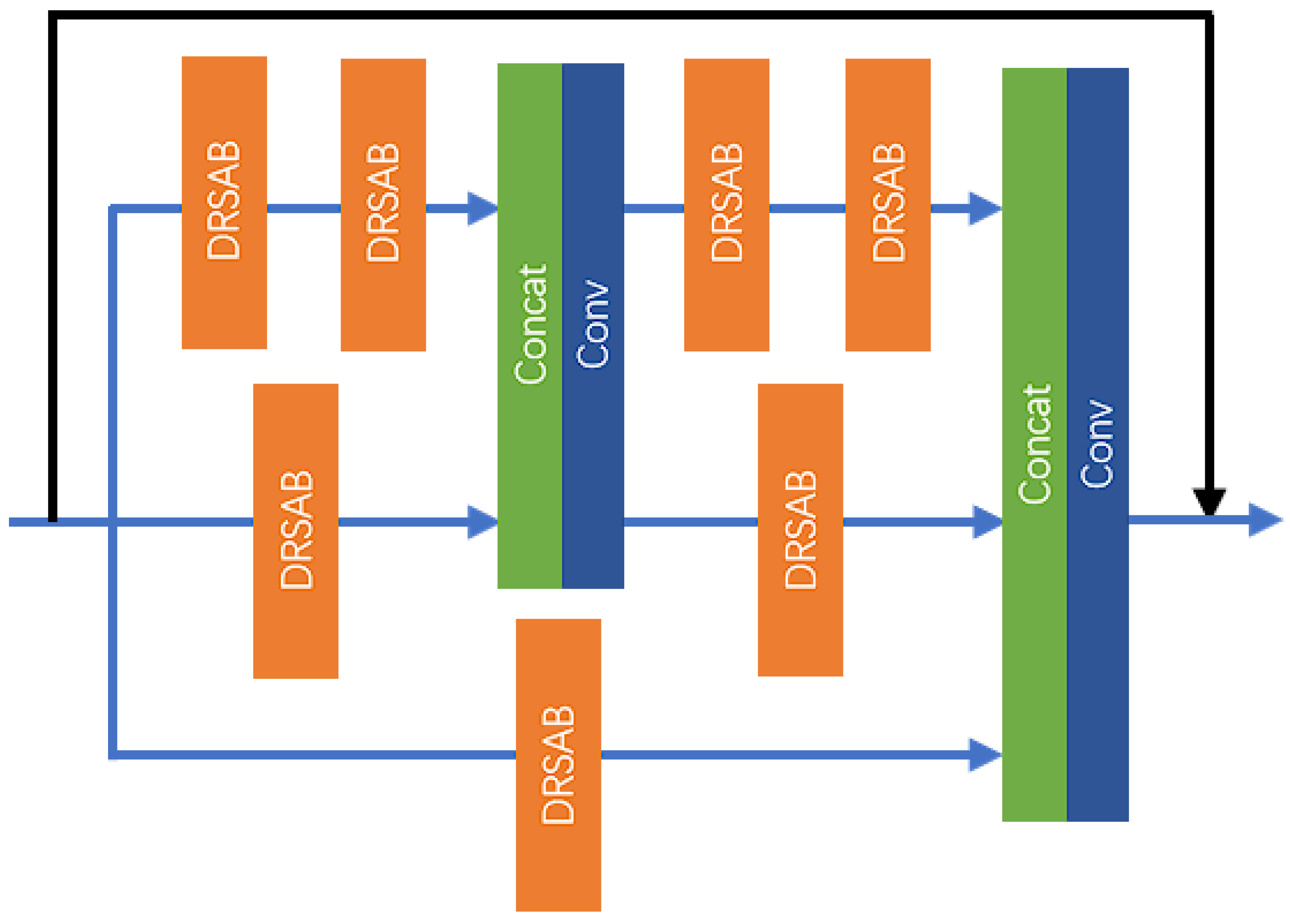
As shown in Figure 3, the MPRB employs a multi-path network along with a residual structure to facilitate feature extraction and fusion at varying depths. The convolutional layer further integrates the output results and extracts features, ultimately producing the final output. This process can be mathematically represented as follows:

Figure 3.
The structure of the MPRB.
In (7) and (8), denotes the output features from the i-th MPRB, while represents the feature mapping relationship of the i-th MPRB. The variable signifies the final output features of the MPFEM.
The MPRB primarily comprises dilated residual SA Blocks (DRSABs), convolutional layers, and concatenation layers, utilizing three paths to extract and fuse image features at different depths. Each path is configured with a varying number of DRSABs, and convolutional layers along with concatenation layers are employed to fuse features of different depths. Neurons in the shallow network layers possess a smaller receptive field, making them more adept at capturing local features of the image. As the number of network layers increases, neurons in the deeper layers can perceive larger areas of the input image, allowing them to capture more global and abstract features. Aggregating shallow and deep features enhances the interaction between spatial information and semantic information, resulting in images generated by the model that are more realistic and accurate.
As illustrated in Figure 3, the number of DRSABs configured for the three paths are 4, 2, and 1, respectively. Additionally, two feature fusions are performed at depths 2 and 4 of the first path, followed by a residual connection to further extract image features. The feature extraction process of the MPRB can be specifically represented as follows:
In (9)–(11), denotes the input features to the MPRB, represents the output features of the j-th DRSAB in the i-th path, while indicates the feature mapping relationship of the j-th DRSAB in the i-th path. The function represents the mapping relationship of the concatenation operation, and signifies the output features after feature fusion.
This process achieves the fusion of the relatively deeper features from the first path and the relatively shallower features from the second path. Subsequently, feature extraction and fusion continue, and the specific process can be outlined as follows:
In (12)–(15), denotes the output features of the MPRB. This process completes the second feature fusion, wherein the first path utilizes two layers of DRSABs, the second path employs one layer of DRSAB, and the third path passes the input features through one layer of DRSAB. Finally, the features at different depths from the three paths are fused together, followed by a residual connection, thereby completing the feature extraction task of the MPRB.
The MPRB consists of multiple DRSABs designed to extract image features at varying depths. The structure of the DRSAB is illustrated in Figure 4.
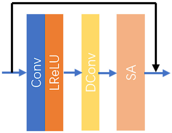
Figure 4.
The structure of the DRSAB.
The DRSAB architecture primarily consists of a convolutional layer, an activation layer, a dilated convolutional layer, and an SA layer. The dilated convolutional layer is a specialized type of convolutional layer that inserts “holes” between the elements of the standard convolution kernel. This design increases the receptive field of the convolutional kernel without adding to the number of parameters or the computational load. Such a mechanism enables the network to capture broader contextual information while maintaining HR and detail, allowing for the extraction of spatial information over a larger area. The SA layer is a specific attention mechanism that enhances the model’s diversity and performance by incorporating random shuffling and grouping during the attention computation process. This form of attention mechanism has significant potential applications in deep learning, particularly in the context of sequence or image data processing. The specific processing steps of the DRSAB are as follows:
In (16)–(18), represents the input features to the DRSAB, denotes the mapping relationship of the convolutional network, and indicates the mapping relationship of the activation function. The output features after activation are represented as . Furthermore, signifies the mapping relationship for the dilated convolution operation, and represents the output features from the dilated convolution. Lastly, denotes the mapping relationship for the SA mechanism, while is the final output result of the DRSAB.
3.1.2. Transformer Feature Enhancement Module
For deep learning-based SR methods, upsampling operations are employed to enlarge LR inputs. Existing methods can generally be categorized into two types based on the position of the upsampling operation: pre-upsampling frameworks and post-upsampling frameworks. Pre-upsampling frameworks were widely adopted in the early stages of deep learning-based SR algorithms. One of the most notable SR models is the SRCNN. This model first performs interpolation (such as bicubic interpolation) on the LR input to enlarge it to the same size as the HR reference. Subsequently, the SR model is utilized to recover the HR image from the interpolated input. The SR model learns the nonlinear mapping between the interpolated LR input and the HR reference, effectively bypassing the upsampling operation, which reduces the learning complexity to some extent. However, for very deep networks, the computation cost increases significantly due to feature extraction occurring in the expanded high-dimensional feature space. To alleviate the high computational cost, some researchers have introduced post-upsampling frameworks to construct end-to-end SR architectures, wherein the entire feature extraction is conducted in a lower-dimensional space. In these frameworks, traditional upsampling methods are replaced with learnable upsampling layers, such as deconvolution [35] and sub-pixel convolution [36], which are integrated into the backend of the network as part of the SR model. Compared to pre-upsampling frameworks, this design significantly reduces computational costs, which is proportional to the square of the preset upscaling factor, allowing a substantial acceleration of the feedforward pass during model training. This architectural design has become mainstream in the field.
However, in this framework, the HR image is directly recovered after the upsampling layer without further enhancement of feature representation. This approach increases the difficulty of training and limits the improvement in reconstruction accuracy, particularly at high upscaling factors. This study employs a transformer-based enhancement network [37], which effectively leverages both low-dimensional and high-dimensional features surrounding the upsampling layers by capturing long-range dependencies, thereby facilitating the exploration of correlations between high-dimensional and low-dimensional features. To further utilize the feature information from the DEM, a three-layer enhancement structure is implemented, consisting of multiple encoders and decoders. Each layer integrates the output features from the multi-perspective feature enhancement module (MPFEM) with high-dimensional features, as illustrated in the accompanying figure. For computational efficiency, prior to entering the transformer-based enhancement network, the input feature image undergoes a reshape operation. The feature image is transformed from a size of to , where and . Here, b denotes the batch size, c represents the number of channels, h indicates the height of the image features, w signifies the width of the image features, and p is a parameter defining the new dimensionality. Each feature enhancement module consists of an encoder and a decoder, with both the encoder and decoder composed of multiple encoder basic modules (EBMs) and decoder basic modules (DBMs), as depicted in Figure 5.
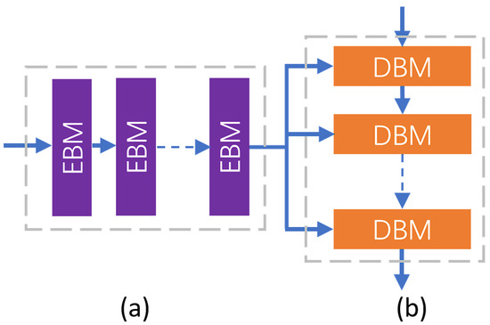
Figure 5.
The structure of the (a) Encoder (b) Decoder.
Here is an example of a one-layer EBM, whose calculation process is as follows:
In (19), represents the output result of the first encoder, while denotes the mapping relationship of the first EBM. The specific structure of the EBM is illustrated in Figure 6.

Figure 6.
The structure of the EBM.
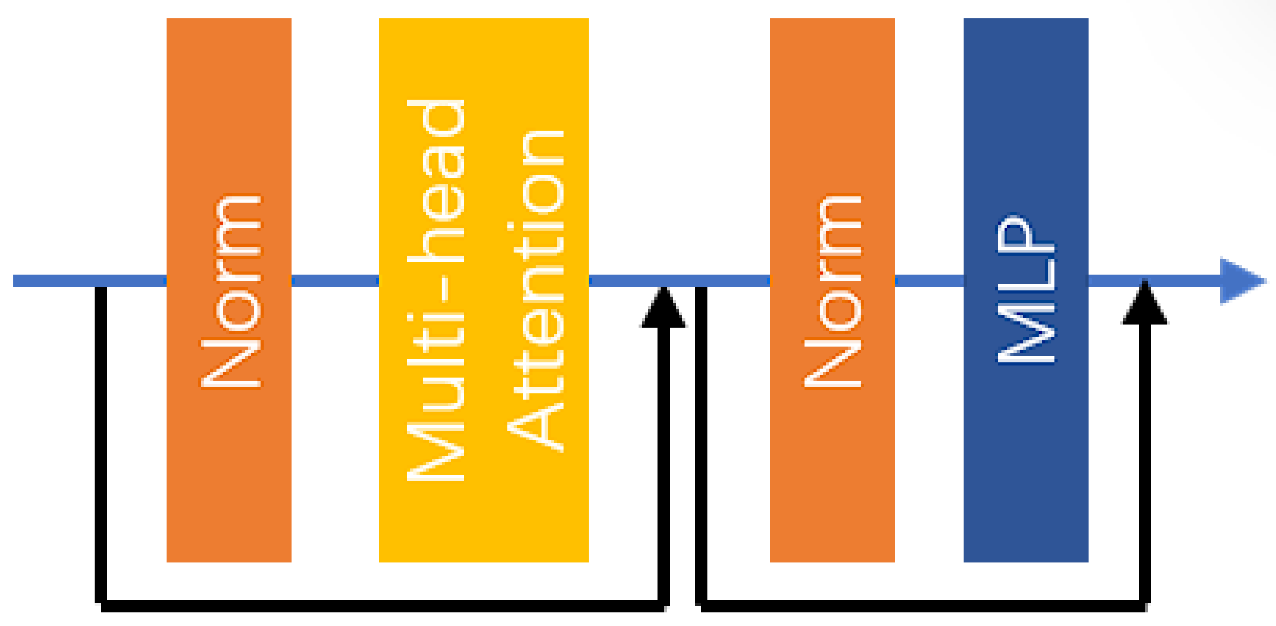
In the EBM, two residual connections, two layer normalization layers, a multi-head attention (MHA) layer, and a multilayer perceptron (MLP) network are utilized. The specific computational process within the EBM is as follows:
In (20)–(23), represents the input image features to the EBM, indicates the mapping relationship of the i-th layer normalization [38]), and is the output image features after the i-th layer normalization. The mapping relationship for the MHA layer is denoted as , while represents the output features after passing through the MHA layer and the residual connection. Lastly, denotes the mapping relationship of the MLP, and is the output features of the EBM.
Layer normalization is a commonly used normalization technique in deep learning. Its computational process can be divided into two parts: normalization and re-scaling. First, normalization is performed on each sample xx across its feature dimensions (or channels). This process can be represented as follows:
In (7), represents the value of the i-th feature in the input x, u is the mean of that feature across all samples, is the variance of that feature, and is a small positive constant used to prevent division by zero. The normalized output is typically multiplied by a learnable scaling parameter and then added to a bias term to produce the final output . This step allows the network to learn to adjust the mean and variance of the data to better suit the task requirements. The formula for the re-scaled output is given by:
The MHA layer is a widely used attention mechanism in deep learning models. This mechanism aims to enhance the model’s expressive power and generalization ability by running multiple independent attention sub-layers in parallel to capture various pieces of information from different parts of the input sequence. The MHA mechanism works by splitting the input sequence into multiple heads, each of which performs its own attention calculation. Specifically, for each head, the model computes attention scores, which allow it to weigh the importance of different parts of the input sequence. The results from these different attention heads are then concatenated and transformed through a linear layer to produce the final output. This approach enables the model to focus on different aspects of the input sequence from various perspectives, capturing more nuanced and hierarchical information. By attending to multiple parts of the input simultaneously, the MHA layer can better understand complex relationships and dependencies within the data, ultimately improving the performance of the model on tasks such as translation, summarization, and other sequence-based applications. The structure of the MHA layer is illustrated in Figure 7.
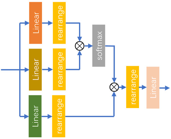
Figure 7.
The structure of the MHA layer.
The MHA mechanism performs linear transformations on the input features through three separate linear layers, mapping them into a higher-dimensional space. This process yields three distinct feature factors, Query, Key, and Value, all of which maintain the same dimensionality. Each attention head possesses its own independent linear transformation, allowing different heads to learn diverse features. The process is as follows:
In (26)–(28), represents the input features of the MHA layer, while denotes the mapping function of the linear layers. Subsequently, the rearrange function is utilized to reorganize each component, partitioning the last dimension of the features into multiple heads according to the specified number of heads.
In (29), represents the mapping function of the rearrange operation, while denotes the features obtained after the linear layer output is transformed. Subsequently, the features and are subjected to a dot product operation using the einsum function. The resulting scores are then passed through a softmax operation for normalization along the last dimension, as detailed in the following process:
In (30) and (31), represents the scaling factor, denotes the mapping function of the einsum operation, and is the result of the dot product operation, which corresponds to the attention weights. Additionally, signifies the mapping function of the softmax operation, while is the output resulting from this softmax operation. After performing the dot product, the attention weights are used to compute a weighted sum of , as described in the following process:
Finally, the rearrange function is applied to merge the attention heads, followed by the use of a linear layer to map the shape of the features back to that of the input feature vector. The process is outlined as follows:
In (33) and (34), represents the output features of the MHA layer. Different heads in the MHA can focus on various parts of the input, capturing a wider array of features and patterns. This capability enhances the model’s ability to capture long-range dependencies and complex structural information, contributing to greater stability and robustness during the learning process.
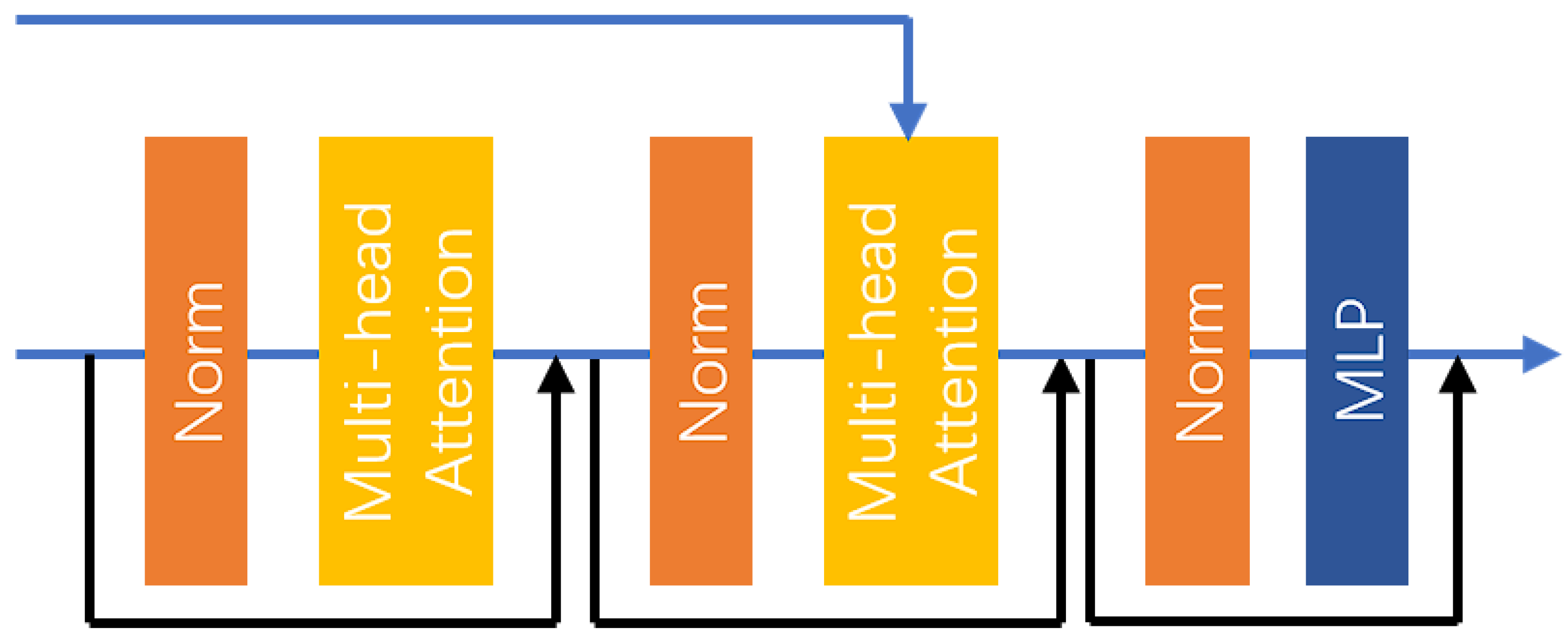
The input characteristics of the DBM are divided into two parts, the first is the output characteristics of the upper layer DBM or the output characteristics of the encoder after the upper sampling layer, and the second is the output characteristics of the corresponding encoder as part of the input of the second layer MHA. The specific structure of the DBM is shown in Figure 8.

Figure 8.
The structure of the DBM.
First, the input features undergo a series of layer normalization layers and an MHA layer, incorporating residual connections. Subsequently, the features pass through another set of layer normalization layers and an MHA layer, which also includes residual connections. However, in this case, the second MHA layer has two input features. As previously mentioned, the MHA layer processes the input features through three linear layers to map them into a new feature space. Here, the output of the encoder serves as the input for the first two linear layers, while the output of the second layer normalization is utilized as the input for the third linear layer. This setup facilitates the fusion of low-dimensional and high-dimensional features, thereby enhancing the accuracy of the reconstruction.
3.2. Loss Function
In this experiment, two loss functions were employed: the mean absolute error (MAE) and the root mean squared error (RMSE).
MAE is a straightforward and intuitive method for measuring the difference between predicted values and actual values. In the context of image SR reconstruction, MAE can be expressed as the average of the absolute pixel differences between the reconstructed image and the original HR image. The specific formula is as follows:
In (35), represents the pixel values of the HR image, denotes the pixel values of the reconstructed image, and n signifies the total number of pixels in the image.
The method used in this study uses RMSE. RMSE is an improved form of the MAE, as it averages the squared pixel errors and then takes the square root, thereby amplifying the impact of larger errors. In the context of image SR reconstruction, RMSE provides a more precise reflection of the pixel differences between the reconstructed image and the original image. The specific formula is as follows:
4. Results
4.1. Experiment Preparation
The experiment involved downloading DEM data from a public geographic service. Specifically, DEM data with a resolution of 20 m from Institut Cartografic i Geologic de Catalunya for parts of Spain based on LiDAR data and photogrammetric means, with an original elevation point density of around 10 and an elevation accuracy of 0.90 m root mean square error, which is used as the HR reference DEM. The LR data are generated by the bi-cubic interpolation downsampling technique. A total of 2955 pairs of DEM images were created, with the HR DEMs sized at pixels and the LR DEMs at pixels. The dataset was randomly divided into training, validation, and testing sets in a ratio of 8:1:1. The study area is characterized by mountainous terrain, which is advantageous as it contains various geological features that are often difficult to preserve in medium-resolution DEMs but are clearly visible in aerial photographs. These features include sharp ridges, boulders, canyons, and glacier crevasses, thereby enhancing the richness of the dataset.
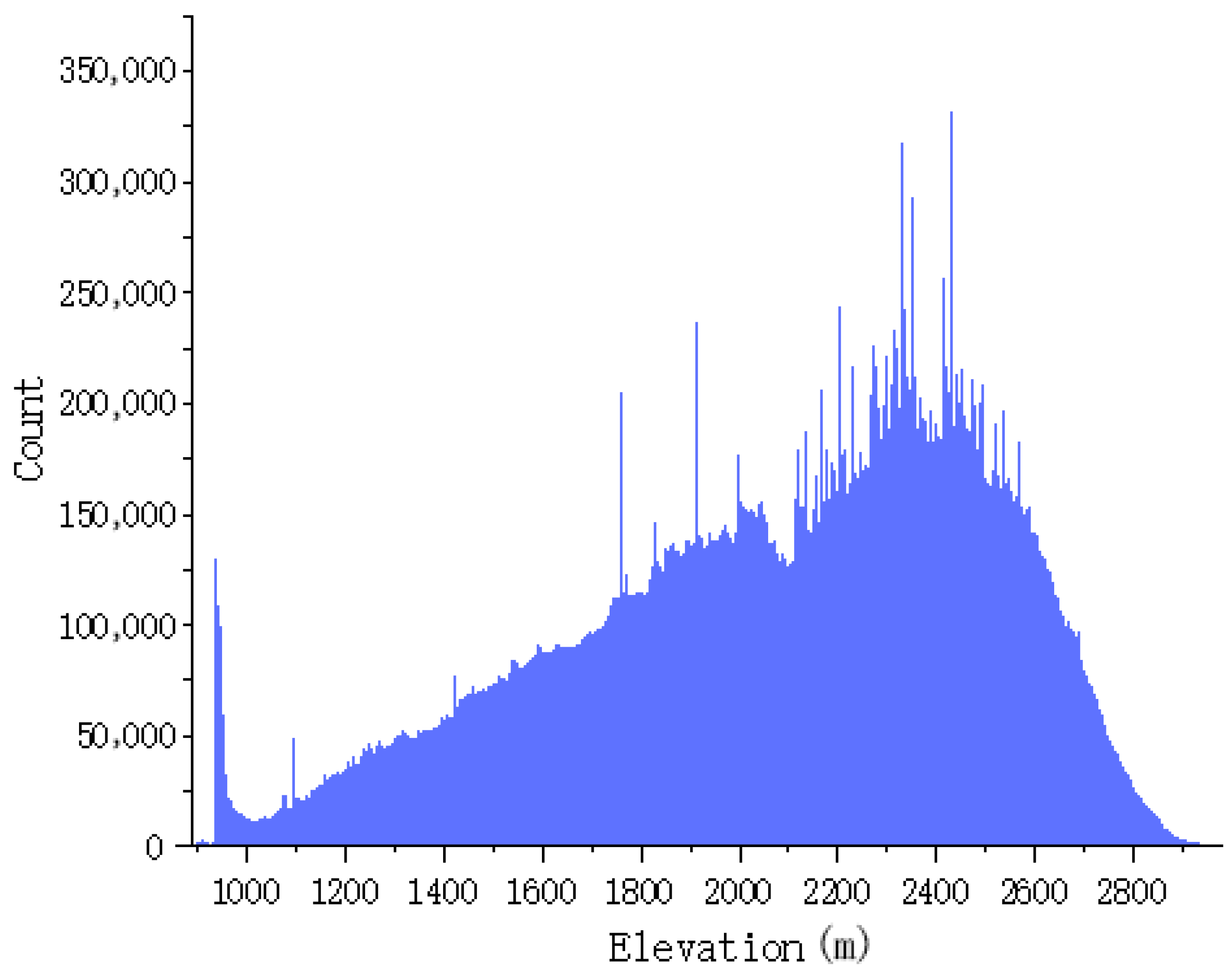
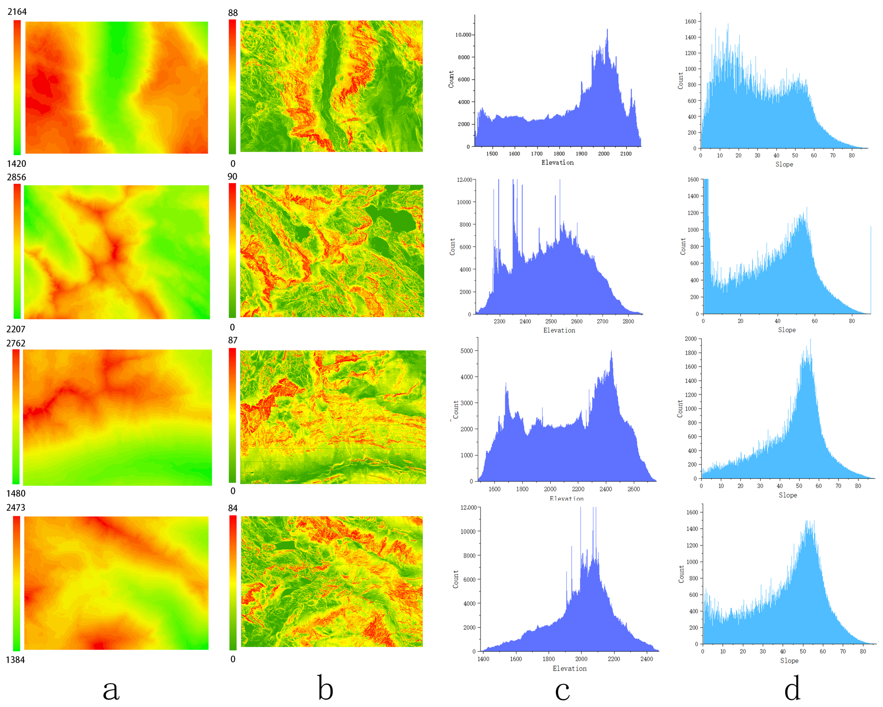
Figure 9 shows that the elevations of the dataset range from 1014 to 2981 m, and the height above sea level ranges mostly from 2000 to 2700 m. Figure 10 shows that the slope range of the study area varies from 0 to 88 degrees, predominantly focusing on the range of 50 to 75 degrees. This region encompasses a variety of complex topographical features, including ridges, valleys, rivers, and cliffs. Figure 11 shows the randomly selected partial data and its distribution within the region.
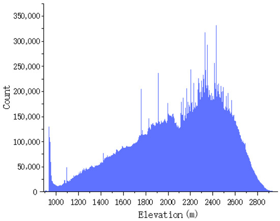
Figure 9.
Elevation distribution of the dataset.
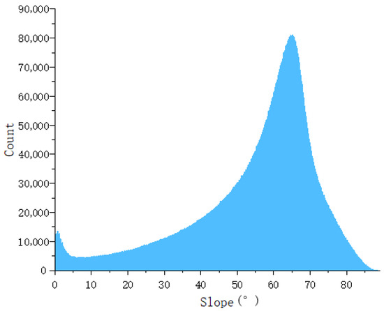
Figure 10.
Slope distribution of the dataset.

Figure 11.
The partial data of the study area are presented as follows: (a) elevation map, (b) slope map, (c) elevation distribution, and (d) slope distribution.
The experiments were conducted using the PyTorch 1.7.0 framework, with a GTX 3060 12 GB GPU configuration. The HR images employed in the study were of size , while the LR images were . The batch size for the input images was set to 10, with all input data being randomly cropped. The Adam optimizer was utilized with parameters set to and . The initial learning rate for training was set to , and the total number of training iterations was . The learning rate was halved at training iterations of and .
4.2. Evaluation Metrics
In this experiment, the evaluation of the effectiveness of DEM SR reconstruction is based on three metrics: elevation, slope, and the structural similarity index measure (SSIM).
Slope is an essential indicator for measuring the degree of inclination of the terrain surface. In the context of DEM SR reconstruction, preserving the slope characteristics of the original topography is crucial for subsequent applications such as terrain analysis and hydrological simulations. By assessing the changes in slope after reconstruction, it is possible to ensure that the primary features of the terrain are accurately retained. Additionally, the calculation of slope relies on the elevation accuracy of the DEM data.
Comparing the slope variations before and after reconstruction can indirectly validate the accuracy and effectiveness of the SR reconstruction algorithm. A minimal change in slope indicates that the reconstruction algorithm performs well in preserving the terrain features. The formula for calculating slope is as follows:
In (37)–(39), represents the elevation value at the i-th row and j-th column of the DEM, while CellSize indicates the spatial resolution of the DEM. denotes the slope value at the same position in the DEM. The specific evaluation methods for elevation and slope data involve assessing the evaluation error and the RMSE to provide a comprehensive assessment of the reconstruction effectiveness.
SSIM is a metric used to assess the similarity between two images, with a particular emphasis on structural information. In the context of DEM SR reconstruction, SSIM can be employed to evaluate the structural similarity between the reconstructed DEM and the original DEM. A high SSIM value indicates that the reconstructed DEM is structurally similar to the original DEM, thereby validating the effectiveness of the reconstruction algorithm. SSIM considers not only the luminance information of the images but also incorporates contrast and structural information. This comprehensive approach allows SSIM to provide a more thorough assessment of the performance of DEM SR reconstruction algorithms. By utilizing SSIM for evaluation, insights can be gained regarding the algorithm’s ability to preserve topographical details and suppress noise. The specific formula for SSIM is as follows:
In (40), and represent the elevation of DEMs x and y, respectively. denotes the covariance between DEM x and y, while and represent the variances of DEM x and y, respectively. and are non-zero constants, where L represents the dynamic range of the elevation of DEMs. The default values for and are set to and , respectively.
4.3. Analysis of Image Quality Metrics During Training Process
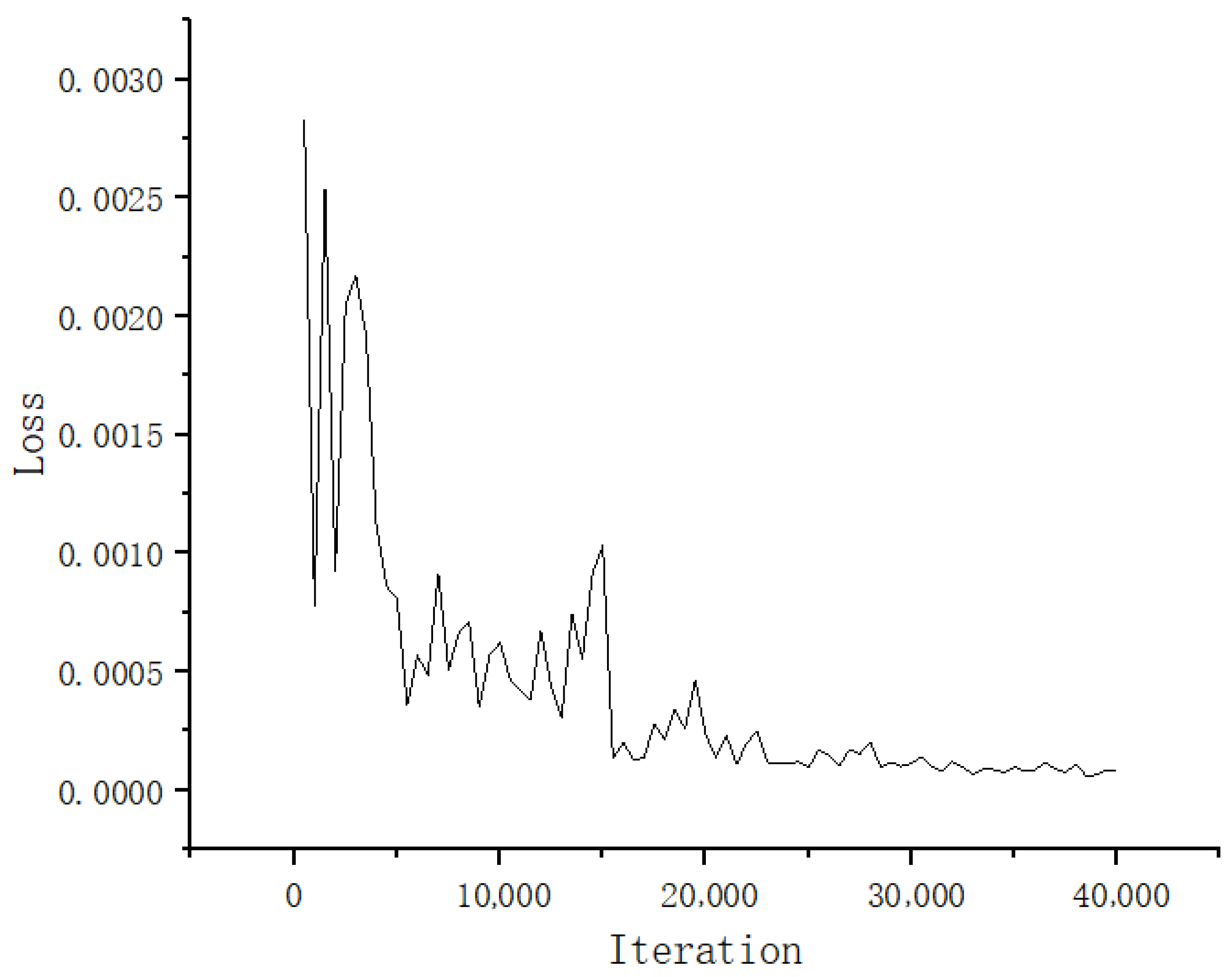
Figure 12 presents the training details, showing the variation in the loss function during the training process. The x-axis represents the number of iterations, while the y-axis indicates the loss value. Figure 12 shows a downward trend with fluctuations in the loss curve during training. In the early stages, there are significant fluctuations with an amplitude around 0.015, and the loss value decreases rapidly. In the mid-training phase, the fluctuation amplitude reduces to about 0.005, with the loss value continuing to decline gradually. In the later stages, the curve becomes increasingly smooth. This phenomenon indicates that our model is effectively capturing the mapping relationships within the dataset, and it gradually converges as training progresses.
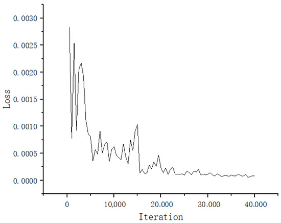
Figure 12.
The curve representing the variation in model loss during training.
4.4. Comparative Experiment
We compared our DEM SR reconstruction method with several other techniques, namely, bicubic interpolation, SRCNN [7], EDSR [11], MFRAN [39], SRGAN [40], ESRGAN [41], and Tfasr [42]. The comparative experiments were conducted under the same conditions, ensuring that the training dataset, number of training iterations, initial learning rate, and training hardware environment remained consistent across all methods.
Table 1 presents the evaluation metrics for different methods tested on the DEM in the test dataset. It can be observed that the GAN-based methods, ESRGAN and SRGAN, exhibit poorer performance in elevation metrics. This is attributed to the instability of generative adversarial training, which makes it challenging to consistently generate accurate DEMs. Among all the methods, the model proposed in this study outperforms in all evaluation metrics, demonstrating its superiority in terms of performance across the various metrics.

Table 1.
The evaluation metrics for different methods tested on the test dataset, with the best-performing metrics highlighted in bold.
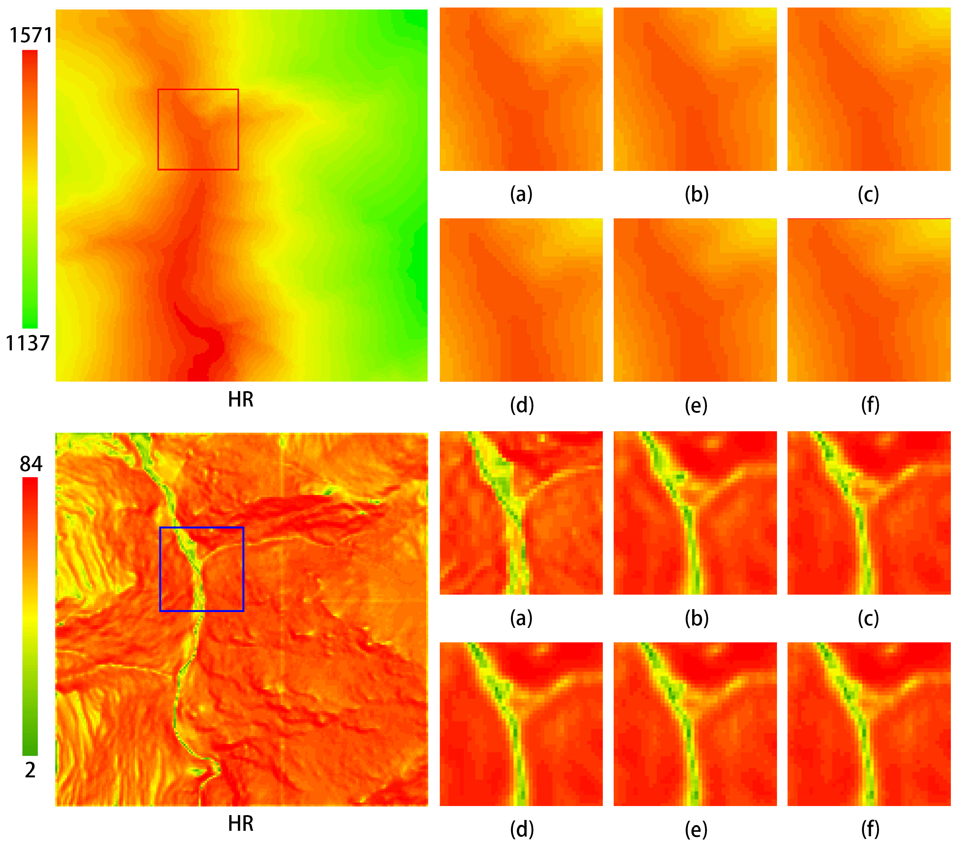
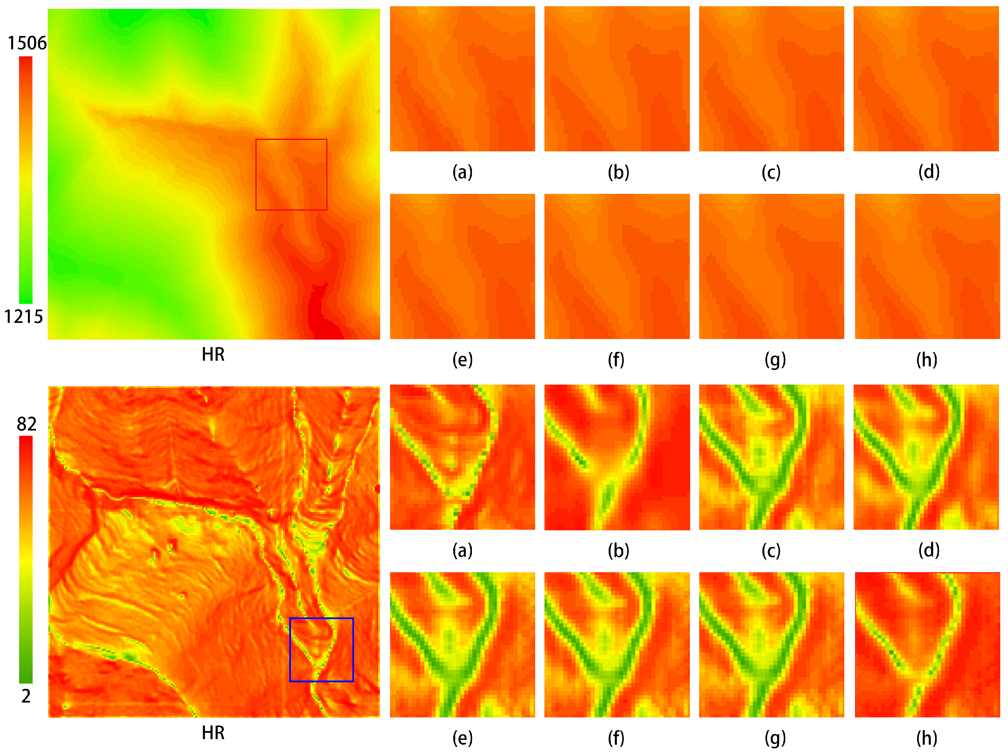
Figure 13 illustrates the comparison of elevation visualization results of different methods on the DEM test dataset. As shown in the figure, the method proposed in this study demonstrates superior visualization performance compared to the aforementioned reconstruction methods. Among these, SRCNN, EDSR, SRGAN, and ESRGAN exhibit suboptimal results, with significant discrepancies in detail compared to the HR image, indicating lower accuracy. Although the image reconstructed using bicubic interpolation is closer to the HR image, it suffers from excessive smoothness, resulting in a loss of detail. The DEM reconstructed by MFRAN and Tfasr shows relatively good performance; however, it falls short in certain details compared to the method proposed in this study. The reconstruction method introduced herein achieves a visual effect for the DEM that is closely aligned with the HR image, demonstrating the best reconstruction accuracy.
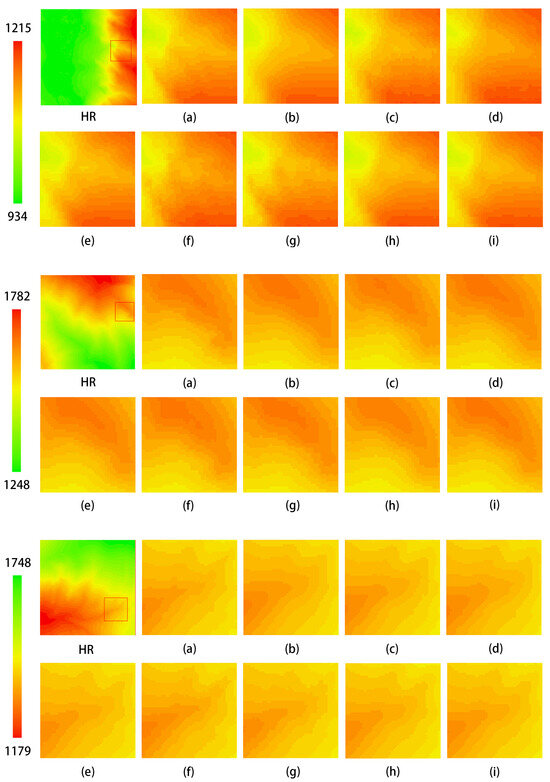
Figure 13.
Comparison of elevation visualization results of different methods on the test dataset. The leftmost image displays the original test dataset, while the other images illustrate local zoomed-in views: (a) HR; (b) Bicubic; (c) SRCNN; (d) EDSR; (e) MFRAN; (f) SRGAN; (g) ESRGAN; (h) Tfasr; (i) Ours.
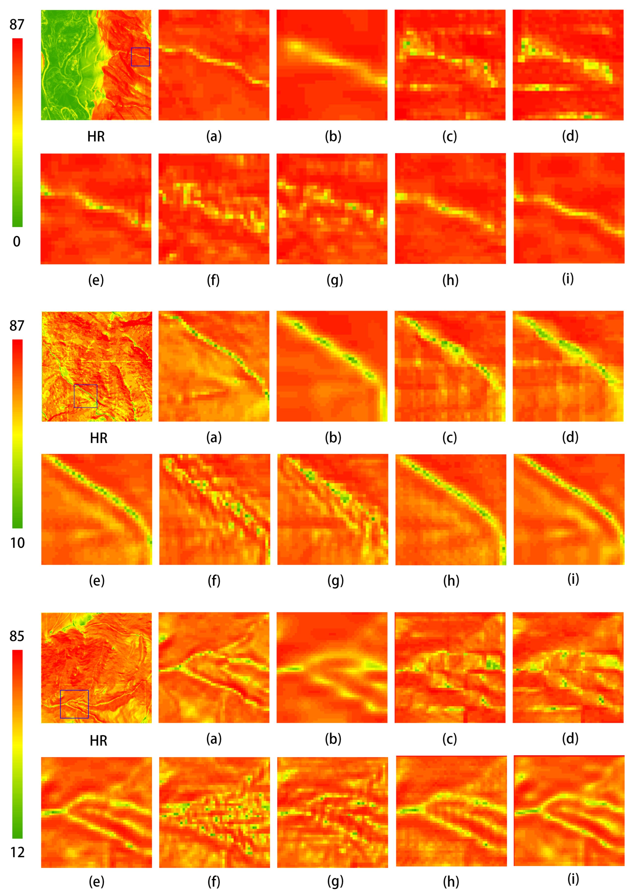
Figure 14 presents a comparison of slope visualization results of different methods on the DEM test dataset. The visualization results indicate that the method proposed in this study outperforms the aforementioned reconstruction techniques in terms of slope accuracy. The precision of slope reconstruction is an essential criterion for evaluating the effectiveness of reconstruction methods. As observed in the three comparison images above, although the slope map reconstructed using bicubic interpolation is generally close to the HR image, it appears somewhat blurred and lacks precision. Methods such as SRCNN, EDSR, SRGAN, and ESRGAN exhibit noticeable discrepancies in the visualization of slope maps compared to the HR image, with some regions of similar slope displaying anomalous artifacts. Notably, the GAN-based methods suffer from instability during adversarial training, resulting in significant differences between the reconstructed slope maps and the original HR images, leading to suboptimal performance. The MFRAN and Tfasr methods provide commendable results in slope reconstruction; however, the method proposed in this study further enhances slope accuracy, demonstrating the best visualization performance.
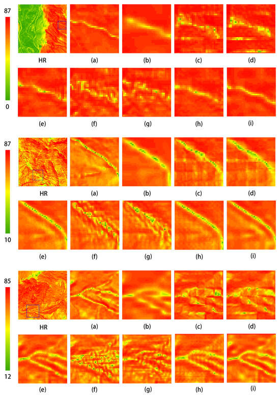
Figure 14.
Comparison of slope visualization results of different methods on the test dataset. The leftmost image displays the original test dataset, while the other images present local zoomed-in views: (a) HR; (b) Bicubic; (c) SRCNN; (d) EDSR; (e) MFRAN; (f) SRGAN; (g) ESRGAN; (h) Tfasr; (i) Ours.
4.5. Ablation Experiment
This study conducted ablation experiments focusing on the MPFEM, the transformer feature enhancement module, and the loss function. Two types of loss functions were evaluated: MAE and RMSE. The optimal loss function was selected based on the experimental results, which are presented in Table 2.
Table 2.
Results of various network performance metrics from the ablation experiments.
As shown in Table 2, the network utilizing the RMSE loss function outperforms the network that employs the MAE loss function to a certain extent. Overall, the combination of the MPFEM, the transformer feature enhancement module, and the RMSE loss function demonstrates the best performance. Figure 15 illustrates that as each module is progressively added to the network, the visual quality of the generated images improves. This outcome provides evidence for the feasibility of the network comprising the MPFEM, the transformer feature enhancement module, and the RMSE loss function.
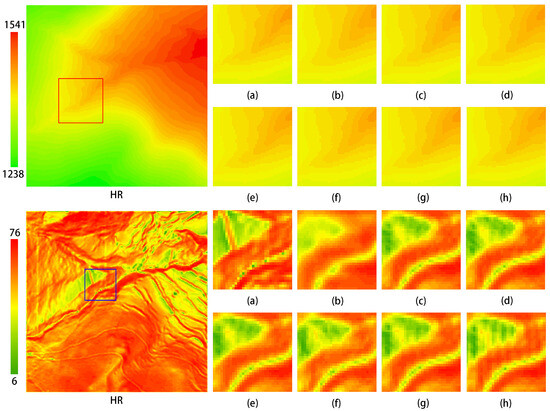
Figure 15.
Ablation experiment test images for each component of the model. The upper section displays the eblevation maps, while the lower section presents the slope maps. (a) HR; (b–h) correspond to the experimental results in Table 2.
The MPRB is a crucial component of the MPFEM. This study conducted ablation experiments focusing on the number of paths in the MPRB and the basic feature extraction modules. Three path configurations were evaluated: 2, 3, and 4. The basic feature extraction modules included the residual block (Res-block), residual dense block (RDB), and DRSAB. The experimental results are presented in Table 3. As indicated in Table 3, the optimal reconstruction metrics were achieved when the basic feature extraction module was DRSAB and the number of paths in the MPRB was set to 3. Figure 16 demonstrates that in the elevation map, the network utilizing the DRSAB proposed in this study yields the best visualization results.
Table 3.
Ablation experiments on basic feature extraction blocks used in MPFEM.

Figure 16.
Visualization results of ablation experiments on the MPFEM. The upper section displays the elevation maps, while the lower section presents the slope maps. The configurations are as follows: (a) HR (b) Res-block + Path-3; (c) RDB + Path-3; (d) DRSAB + Path-2; (e) DRSAB + Path-3; (f) DRSAB + Path-4.
The transformer feature enhancement module consists of an encoder and a decoder, where the encoder is composed of multiple layers of EBMs and the decoder consists of multiple layers of DBMs. This study conducted ablation experiments to evaluate the number of layers in both the EBMs and DBMs. The number of EBM layers was selected as 2, 4, 6, and 8, while the number of DBM layers was chosen as 1, 2, 3, and 4. The experimental results are presented in Table 4. As indicated in these tables, the network performs best when the number of EBM layers is set to 8 and the number of DBM layers is set to 2, yielding optimal metrics for the reconstructed DEM. Figure 17 demonstrates that the best visualization results are achieved when the encoder and decoder layers are configured as 8-2, particularly evident in the slope maps.
Table 4.
Ablation experiments related to the transformer feature enhancement module.
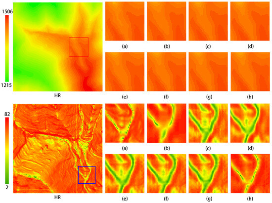
Figure 17.
Visualization results of ablation experiments on the transformer feature enhancement module. The upper section displays the elevation maps, while the lower section presents the slope maps. (a) HR (b) Bicubic (c–h) correspond to configurations with the EBM and DBM layer counts of 3-2, 4-2, 6-2, 8-1, 8-3, and 8-2, respectively.
5. Discussion
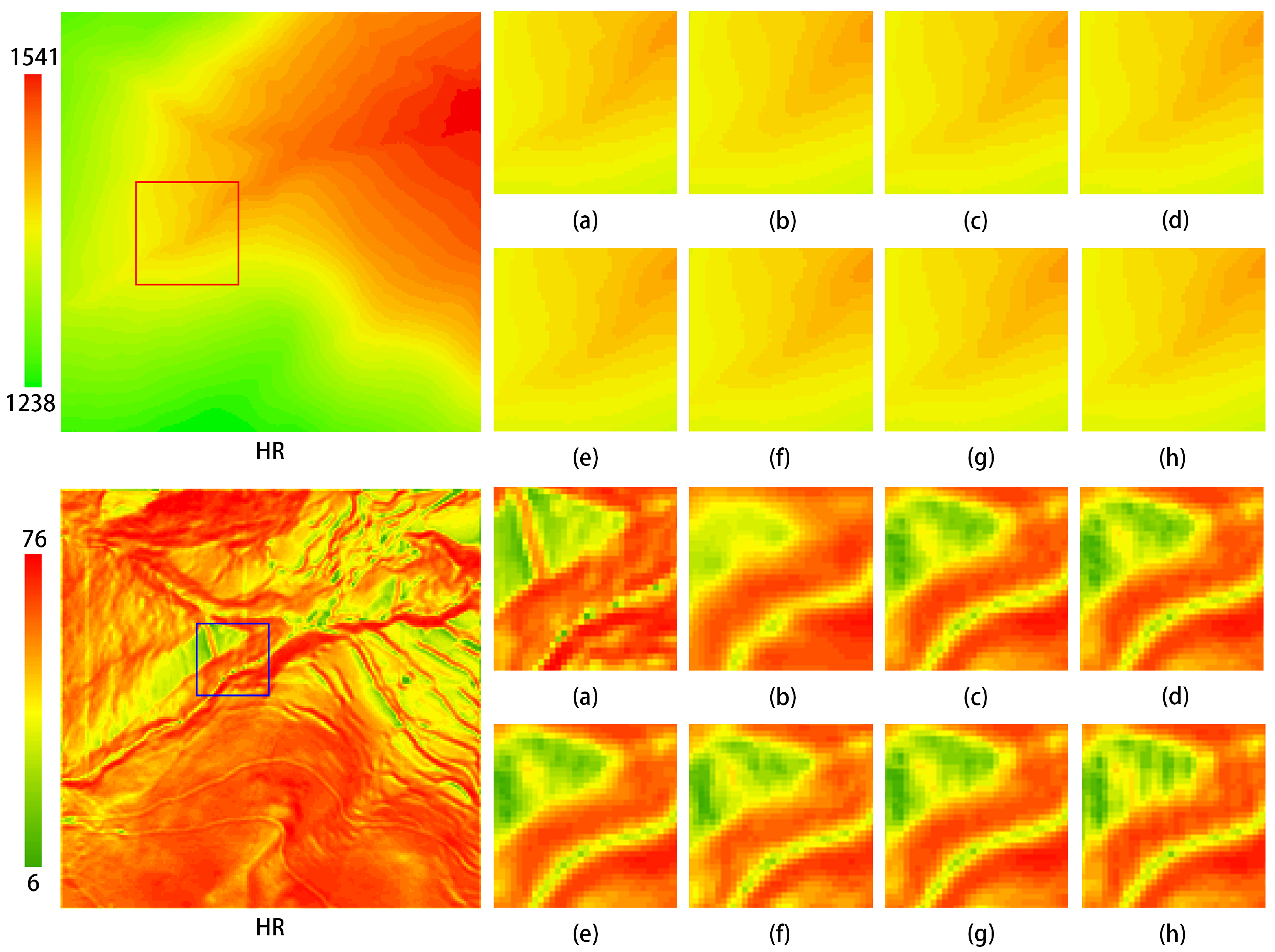
To further validate the performance of the model, this experiment utilized a dataset derived from Mars DEM data. These data were sourced from the Astrogeology Science Center of the United States Geological Survey (USGS) to support the landing and navigation of the Perseverance rover. The provided DEM data, with a resolution of 20 m, captures subtle variations in the Martian surface, including features such as ridges, canyons, and steep slopes. HR images were downsampled to obtain LR images, which were then randomly divided into three parts in an 8:1:1 ratio through cropping, providing the model with training, inference, and testing datasets. The experimental results are presented in Table 5 and Figure 18, demonstrating that the model proposed in this study achieves commendable reconstruction performance on this dataset.
Table 5.
The evaluation metrics for the different methods tested on the Mars DEM dataset are shown below, with the best performing metrics highlighted in bold.
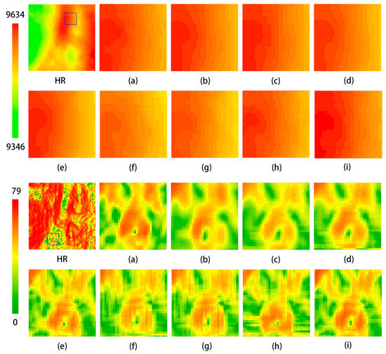
Figure 18.
Comparison of visualization effects of different methods on Mars DEM dataset. The far-left image shows the original image from the test dataset, while the others are local zoomed-in views. (a) HR; (b) Bicubic; (c) SRCNN; (d) EDSR; (e) MFRAN; (f) SRGAN; (g) ESRGAN; (h) Tfasr; (i) Ours.
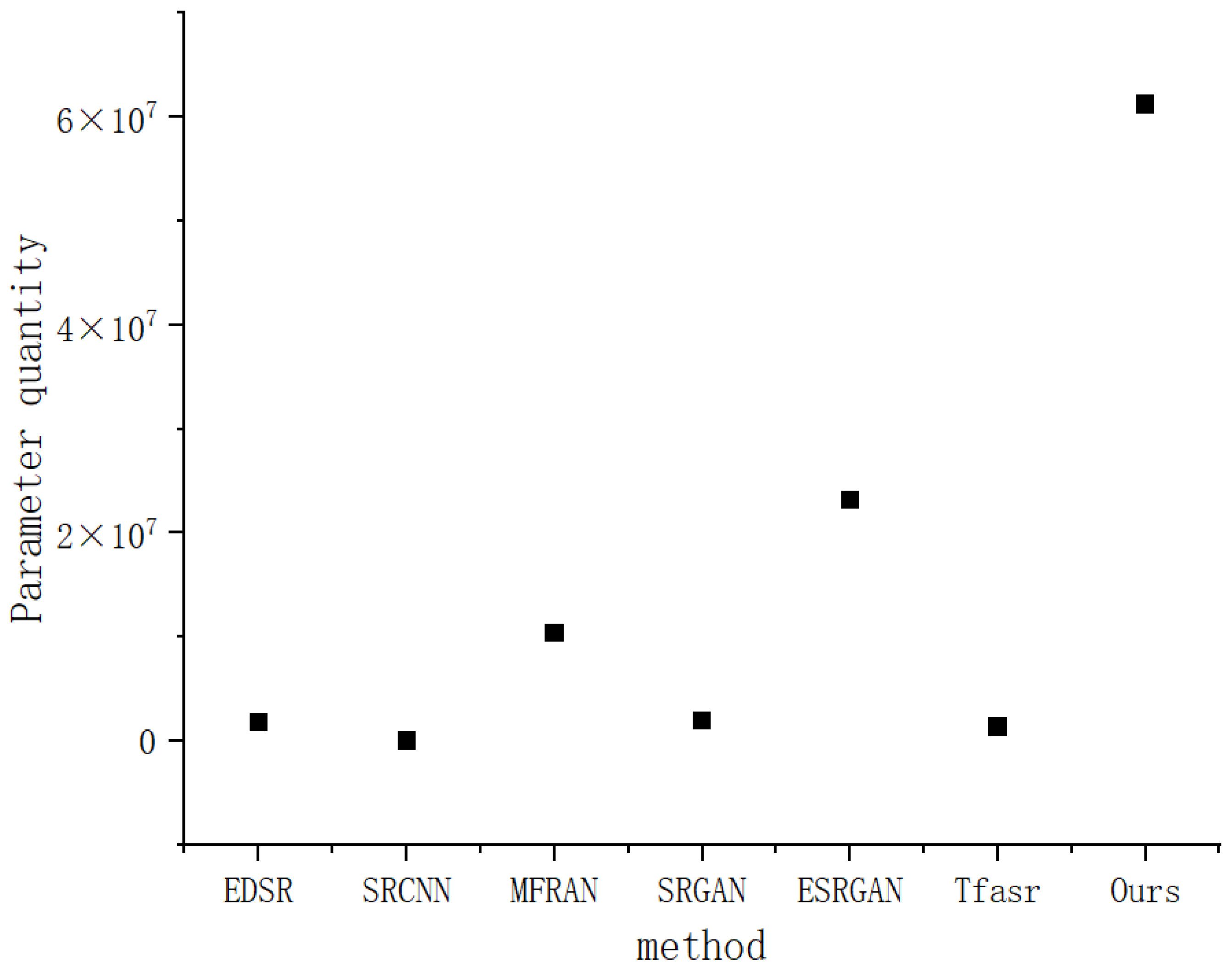
To further understand our method, the model parameters and reconstruction speed are compared below.
Figure 19 shows the number of parameters of various topographic data super-resolution reconstruction methods. The horizontal coordinate lists different methods, namely, EDSR, SRCNN, MFIFAN, SRGAN, ESRGAN, Tfsacr, and the method proposed in this paper; The ordinate represents the number of parameters in scientific notation. It can be clearly seen from the figure that the number of parameters of our method is significantly higher than that of other methods, reaching 6.00 , which is far higher than the second-highest ESRGAN (about 2.00 ). The number of parameters in the other methods is relatively small and the values are similar. This shows that our method is far superior to the comparison method in model complexity.
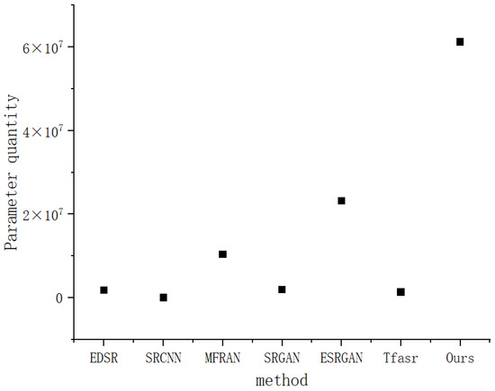
Figure 19.
Comparison of number of model parameters.
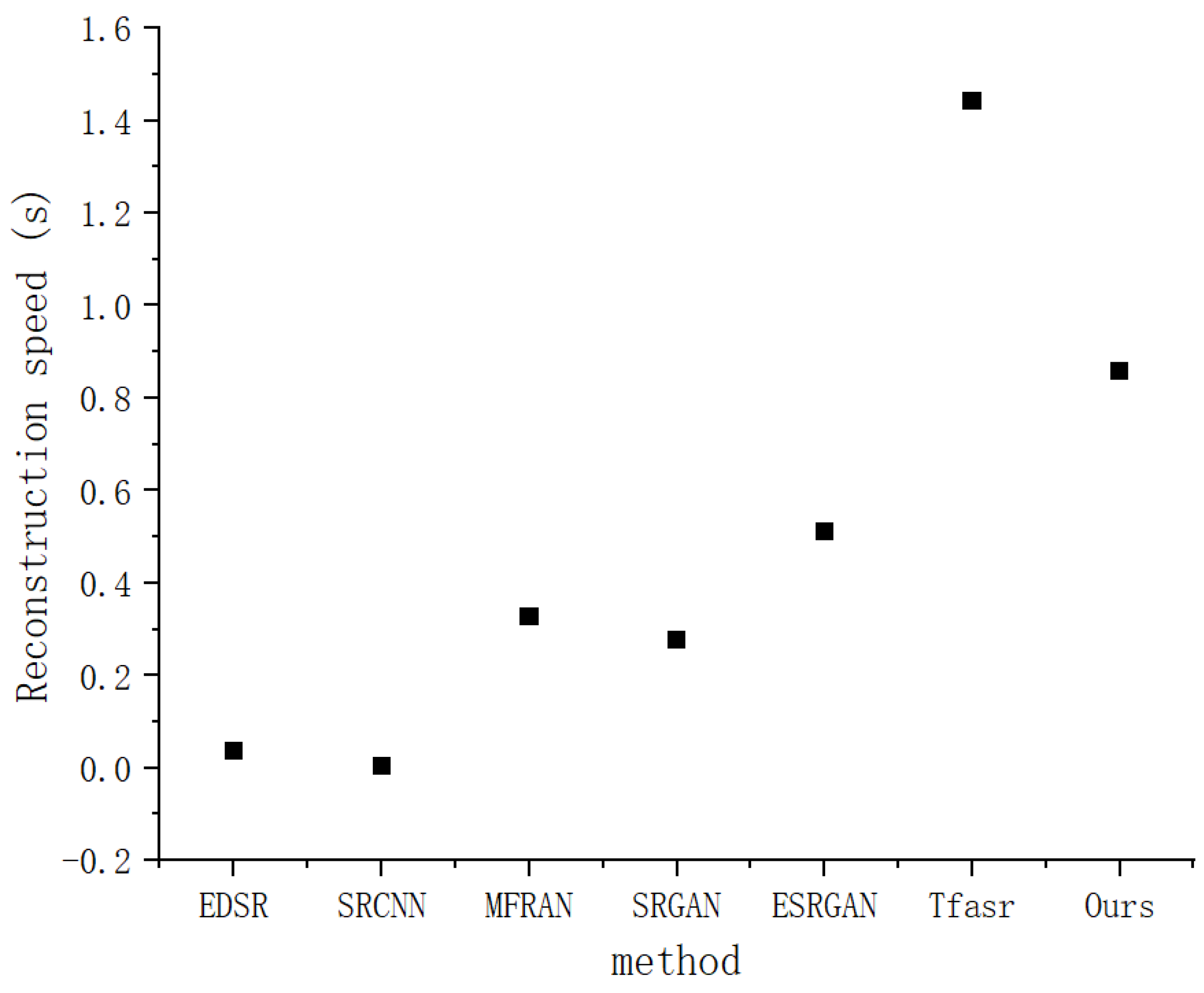
Figure 20 shows the super-resolution reconstruction speed of terrain data by each method. The horizontal coordinate is once again the different methods, and the vertical coordinate is reconstruction speed, in seconds (s). Among them, the Tfsacr method has the slowest reconstruction speed, which is between 1.4 and 1.6 s. The reconstruction speed of our method is also relatively slow, ranging from 0.8 to 1.0 s. The reconstruction speeds of EDSR and SRCNN are the fastest, which is between 0 and 0.2 s. The reconstruction speeds of MFIFAN and SRGAN are similar, ranging from 0.2 to 0.4 s, while that of ESRGAN is about 0.4–0.6 s. This demonstrates that our method is not superior to these comparative methods in terms of reconstruction speed.
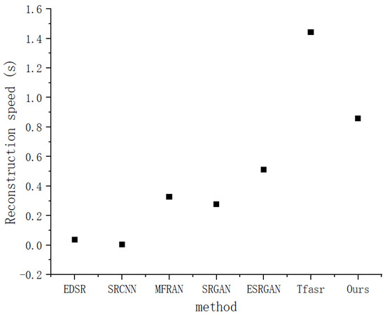
Figure 20.
Reconstruction speed.
Although the method proposed in this paper demonstrates certain advantages in terrain data super-resolution reconstruction, the limitations revealed by the above two maps require more in-depth and systematic discussion. Firstly, regarding the parameter quantity, our method exhibits a significantly higher number of parameters compared to other comparative methods. This is primarily attributed to the incorporation of the transformer architecture. Transformers rely on self-attention mechanisms, which introduce a large number of learnable parameters for calculating attention weights between different elements in the terrain data sequence. Each attention head needs to learn its own set of weight matrices, and multiple attention heads further increase the parameter count. As a result, the model complexity escalates substantially. The high parameter count not only demands an excessive amount of computational resources during training, thereby increasing training costs and extending the training time, but also poses a risk of overfitting. This reduces the generalization ability of the model when encountering new and unknown terrain data. Secondly, in terms of reconstruction speed, our method is relatively slow. The transformer-based architecture, while powerful in capturing global dependencies in terrain data, comes with a high computational cost. The self-attention calculations are computationally intensive, as they involve matrix multiplications with quadratic complexity in relation to the sequence length of the terrain data. When dealing with large-scale terrain data, these repeated matrix operations significantly slow down the reconstruction process. This limitation restricts the practical application of the method, especially in scenarios with stringent real-time requirements, such as real-time terrain data monitoring and rapid terrain data updates.
6. Conclusions
This paper presents a systematic study and discussion on the SR reconstruction methods for DEMs. After analyzing the current mainstream technologies and their application contexts, we propose a deep learning-based framework for DEM SR reconstruction aimed at enhancing the spatial resolution of DEMs. This paper makes several significant contributions to the field of DEM super-resolution reconstruction. First, a novel super-resolution reconstruction network for DEMs is proposed, integrating multi-path feature extraction and transformer feature enhancement. Experimental results demonstrate that this method outperforms existing super-resolution techniques, enabling the reconstruction of high-accuracy high-resolution DEMs. Second, the MPFEM is introduced, which consists of MPRBs. By leveraging multipath extraction, extended convolution layers, and SA layers, MPFEM effectively enhances the interaction between spatial and semantic information, optimizing the feature extraction process. Third, a transformer-based feature enhancement module is developed. Comprising multiple encoders and decoders, this module processes the output of each feature extraction module, facilitating the fusion of high- and low-dimensional features and significantly improving the overall performance of the network. These contributions provide new perspectives and effective solutions for terrain data super-resolution reconstruction.
However, despite the achievements of this study, there remain many challenges and opportunities for improvement in the field of DEM SR reconstruction. Future research could focus on the following aspects: addressing the computational complexity of current deep learning models by exploring more efficient network architectures and training strategies to enhance model performance in large-scale DEM processing; investigating fusion methods for different data sources (such as remote sensing imagery, meteorological data, etc.) to achieve more accurate terrain reconstruction and enhance the model’s generalization ability; deeply exploring the potential of SR reconstruction in practical applications, such as natural disaster monitoring, urban planning, and environmental protection, to facilitate the transition of technology to real-world scenarios; and strengthening the research on the interpretability of deep learning models to increase user trust and acceptance of model results, thereby promoting their application in practice.
Further research can be conducted on the issue of DEM super-resolution reconstruction results exceeding or falling below the original data range. On the one hand, adaptive algorithms based on deep learning will continue to optimize by constructing more complex neural network structures, automatically learning data features and range boundaries, and achieving precise constraints on reconstruction results; On the other hand, multi-source heterogeneous data fusion will play a greater role, combining multi-source information such as satellite remote sensing, unmanned aerial vehicle mapping, LiDAR point clouds, etc., to establish a dynamic data correction model and intelligently correct outliers in real time. In addition, by combining virtual reality and digital twin technology, abnormal data can be interactively processed in a 3D visualization environment, making the processing process more intuitive and efficient.
In addition, it is of great significance to determine the feasible landscape types for the super-resolution reconstruction of topographic data. Different landscape types, such as mountains, plains, river valleys, and forests, have different topographic characteristics. If a method can effectively reconstruct high-resolution topographic data under different landscapes, this indicates that the method has a wider application range and better generalization ability. Of course, there are also factors related to landscape type that can affect the improvement in resolution. In mountainous areas, the presence of sharp peaks and deep valleys means that more detailed elevation information is needed. This method can make use of geometric features such as the slope relation of the mountain to improve the resolution. By accurately capturing these features, the algorithm can interpolate and reconstruct topographic data more precisely. In a valley landscape, the direction of water flow and the shape of the valley floor are crucial. Consideration of hydraulic characteristics associated with river valleys, such as riverbed slope, can improve the resolution of topographic data in these areas. For forest landscapes, topographic-related canopy height models can be incorporated into the super-resolution process. The height and density of trees in the forest affect the surface elevation perception. This method can better reconstruct the underlying terrain with higher resolution by integrating forest-related data.
In summary, the methods for DEM SR reconstruction hold broad research prospects and application value.
Author Contributions
M.G. and F.X. designed the network architecture and conducted comparative and ablation experiments. Y.H. and Z.Z. analyzed and summarized the experimental results data and visualization images, M.G. and F.X wrote the manuscript. Y.H., Z.Z. and J.Z. provided reliable suggestions during the paper revision process. All authors have read and agreed to the published version of the manuscript.
Funding
This work was funded by the National Major Science and Technology Projects of China (2024ZD1002006), National Natural Science Foundation of China (41971356), and the Open Fund of Key Laboratory of Urban Land Resources Monitoring and Simulation, Ministry of Natural Resources, Wuhan East Lake New Technology Development Zone under projects 2024KJB350 and 2024KJB347.
Informed Consent Statement
The study did not involve humans.
Data Availability Statement
No new datasets were created or analyzed.
Conflicts of Interest
Author Ying Huang was employed by the company Wuhan Zondy Cyber Technology Co., Ltd. The remaining authors declare that the research was conducted in the absence of any commercial or financial relationships that could be construed as a potential conflict of interest.
References
- Li, Y.; Gao, F.; Li, W.; Zhang, P.; Yuan, A.; Zhong, X.; Zhai, Y.; Yang, Y. A high-resolution satellite DEM filtering method assisted with building segmentation. Photogramm. Eng. Remote Sens. 2021, 87, 421–430. [Google Scholar] [CrossRef]
- Dongchen, E.; Zhou, C.; Liao, M. Application of SAR interferometry on DEM generation of the Grove Mountains. Photogramm. Eng. Remote Sens. 2004, 70, 1145–1149. [Google Scholar] [CrossRef]
- Aguilar, F.J.; Agüera, F.; Aguilar, M.A.; Carvajal, F. Effects of terrain morphology, sampling density, and interpolation methods on grid DEM accuracy. Photogramm. Eng. Remote Sens. 2005, 71, 805–816. [Google Scholar] [CrossRef]
- Zhang, Y.; Zheng, Z.; Luo, Y.; Zhang, Y.; Wu, J.; Peng, Z. A CNN-based subpixel level DSM generation approach via single image super-resolution. Photogramm. Eng. Remote Sens. 2019, 85, 765–775. [Google Scholar] [CrossRef]
- Boucher, A.; Kyriakidis, P.C. Integrating fine scale information in super-resolution land-cover mapping. Photogramm. Eng. Remote Sens. 2007, 73, 913–921. [Google Scholar] [CrossRef]
- Wang, Z.; Chen, J.; Hoi, S.C. Deep learning for image super-resolution: A survey. IEEE Trans. Pattern Anal. Mach. Intell. 2020, 43, 3365–3387. [Google Scholar] [CrossRef] [PubMed]
- Dong, C.; Loy, C.C.; He, K.; Tang, X. Image super-resolution using deep convolutional networks. IEEE Trans. Pattern Anal. Mach. Intell. 2014, 38, 295–307. [Google Scholar] [CrossRef] [PubMed]
- Dong, C.; Loy, C.C.; Tang, X. Accelerating the Super-Resolution Convolutional Neural Network. In Proceedings of the Computer Vision—ECCV 2016, Amsterdam, The Netherlands, 11–14 October 2016; Proceedings, Part II. pp. 391–407. [Google Scholar]
- Xu, L.; Ren, J.S.J.; Liu, C.; Jia, J. Deep Convolutional Neural Network for Image Deconvolution. Adv. Neural Inf. Process. Syst. 2014, 27, 1905–1914. [Google Scholar]
- Kim, J.; Lee, J.K.; Lee, K.M. Deeply-Recursive Convolutional Network for Image Super-Resolution. In Proceedings of the IEEE Conference on Computer Vision and Pattern Reco Gnition, Las Vegas, NV, USA, 27–30 June 2016; pp. 1637–1645. [Google Scholar]
- Lim, B.; Son, S.; Kim, H.; Nah, S.; Lee, K.M. Enhanced Deep Residual Networks for Single Image Super-Resolution. In Proceedings of the IEEE Conference on Computer Vision and Pattern Recognition (CVPR) Workshops, Honolulu, HI, USA, 21–26 July 2017; pp. 1132–1140. [Google Scholar]
- He, K.; Zhang, X.; Ren, S.; Sun, J. Deep Residual Learning for Image Recognition. In Proceedings of the IEEE Conference on Computer Vision and Pattern Reco Gnition, Las Vegas, NV, USA, 27–30 June 2016; pp. 770–778. [Google Scholar]
- Xu, Z.K.; Wang, X.W.; Chen, Z.X.; Xiong, D.P.; Ding, M.Y.; Hou, W.G. Nonlocal similarity based DEM super resolution. Isprs J. Photogramm. Remote Sens. 2015, 110, 48–54. [Google Scholar] [CrossRef]
- Burrough, P.A.; McDonnell, R.A.; Lloyd, C.D. Principles of Geographical Information Systems; Oxford University Press: New York, NY, USA, 2015. [Google Scholar]
- Yue, L.; Shen, H.; Yuan, Q.; Zhang, L. Fusion of multi-scale DEMs using a regularized super-resolution method. Int. J. Geogr. Inf. Sci. 2015, 29, 2095–2120. [Google Scholar] [CrossRef]
- Argudo, O.; Chica, A.; Andujar, C. Terrain super-resolution through aerial imagery and fully convolutional networks. Comput. Graph. Forum 2018, 37, 101–110. [Google Scholar] [CrossRef]
- Zhang, R.; Bian, S.; Li, H. RSPCN: Super-resolution of digital elevation model based on recursive sub-pixel convolutional neural networks. ISPRS Int. J. Geo-Inf. 2020, 10, 501. [Google Scholar] [CrossRef]
- Zhou, A.; Chen, Y.; Wilson, J.P.; Su, H.; Xiong, Z.; Cheng, Q. An enhanced double-filter deep residual neural network for generating super resolution DEMs. Remote Sens. 2021, 13, 3089. [Google Scholar] [CrossRef]
- Lin, X.; Zhang, Q.; Wang, H.; Yao, C.; Chen, C.; Cheng, L.; Li, Z. A DEM super-resolution reconstruction network combining internal and external learning. Remote Sens. 2022, 14, 2181. [Google Scholar] [CrossRef]
- Han, X.; Ma, X.; Li, H.; Chen, Z. A global-information-constrained deep learning network for digital elevation model super-resolution. Remote Sens. 2023, 15, 305. [Google Scholar] [CrossRef]
- Yao, S.; Cheng, Y.; Yang, F.; Mozerov, M.G. A continuous digital elevation representation model for DEM super-resolution. ISPRS J. Photogramm. Remote Sens. 2024, 208, 1–13. [Google Scholar] [CrossRef]
- Guo, M.; Liu, H.; Xu, Y.; Huang, Y. Building extraction based on U-Net with an attention block and multiple losses. Remote Sens. 2020, 12, 1400. [Google Scholar] [CrossRef]
- Burt, P.J.; Adelson, E.H. The Laplacian pyramid as a compact image code. In Readings in Computer Vision; Morgan Kaufmann: Burlington, MA, USA, 1987; pp. 671–679. [Google Scholar]
- Lindeberg, T. Scale-space theory: A basic tool for analyzing structures at different scales. J. Appl. Stat. 1994, 21, 225–270. [Google Scholar] [CrossRef]
- Krizhevsky, A.; Sutskever, I.; Hinton, G.E. ImageNet classification with deep convolutional neural networks. Adv. Neural Inf. Process. Syst. 2017, 60, 84–90. [Google Scholar] [CrossRef]
- Li, J.; Fang, F.; Mei, K.; Zhang, G. Multi-scale residual network for image super-resolution. In Proceedings of the European Conference on Computer Vision (ECCV), Munich, Germany, 8–14 September 2018; pp. 517–532. [Google Scholar]
- Qin, J.; Huang, Y.; Wen, W. Multi-scale feature fusion residual network for single image super-resolution. Neurocomputing 2020, 379, 334–342. [Google Scholar] [CrossRef]
- Zhang, D.; Shao, J.; Liang, Z.; Liu, X.; Shen, H.T. Multi-Branch Networks for Video Super-Resolution with Dynamic Reconstruction Strategy. IEEE Trans. Circuits Syst. Video Technol. 2021, 31, 3954–3966. [Google Scholar] [CrossRef]
- Feng, X.; Li, X.; Li, J. Multi-scale fractal residual network for image super-resolution. Appl. Intell. 2021, 51, 1845–1856. [Google Scholar] [CrossRef]
- Lv, X.; Wang, C.; Fan, X.; Leng, Q.; Jiang, X. A novel image super-resolution algorithm based on multi-scale dense recursive fusion network. Neurocomputing 2022, 489, 98–111. [Google Scholar] [CrossRef]
- Yang, F.; Yang, H.; Fu, J.; Lu, H.; Guo, B. Learning texture transformer network for image super-resolution. In Proceedings of the IEEE/CVF Conference on Computer Vision and Pattern Recognition, Seattle, WA, USA, 13–19 June 2020; pp. 5791–5800. [Google Scholar]
- Lu, Z.; Liu, H.; Li, J.; Zhang, L. Efficient transformer for single image super-resolution. arXiv 2021, arXiv:2108.11084. [Google Scholar]
- Liu, Z.; Lin, Y.; Cao, Y.; Hu, H.; Wei, Y.; Zhang, Z.; Lin, S.; Guo, B. Swin transformer: Hierarchical vision transformer using shifted windows. In Proceedings of the IEEE/CVF International Conference on Computer Vision, Montreal, BC, Canada, 11–17 October 2021; pp. 10012–10022. [Google Scholar]
- Liang, J.; Cao, J.; Sun, G.; Zhang, K.; Van Gool, L.; Timofte, R. Swinir: Image restoration using swin transformer. In Proceedings of the IEEE/CVF International Conference on Computer Vision, Montreal, BC, Canada, 11–17 October 2021; pp. 1833–1844. [Google Scholar]
- Zeiler, M.D.; Fergus, R. Visualizing and understanding convolutional networks. In Proceedings of the Computer Vision—ECCV 2014: 13th European Conference, Zurich, Switzerland, 6–12 September 2014; Proceedings, Part I 13. pp. 818–833. [Google Scholar]
- Shi, W.; Caballero, J.; Huszár, F.; Totz, J.; Aitken, A.P.; Bishop, R.; Rueckert, D.; Wang, Z. Real-time single image and video super-resolution using an efficient sub-pixel convolutional neural network. In Proceedings of the IEEE Conference on Computer Vision and Pattern Recognition, Las Vegas, NV, USA, 27–30 June 2016; pp. 1874–1883. [Google Scholar]
- Lei, S.; Shi, Z.; Mo, W. Transformer-based multistage enhancement for remote sensing image super-resolution. IEEE Trans. Geosci. Remote Sens. 2021, 60, 1–11. [Google Scholar] [CrossRef]
- Lei Ba, J.; Kiros, J.R.; Hinton, G.E. Layer normalization. arXiv 2016, arXiv:1607.06450. [Google Scholar]
- Song, X.; Liu, W.; Liang, L.; Shi, W.; Xie, G.; Lu, X.; Hei, X. Image super-resolution with multi-scale fractal residual attention network. Comput. Graph. 2023, 113, 21–31. [Google Scholar] [CrossRef]
- Ledig, C.; Theis, L.; Huszár, F.; Caballero, J.; Cunningham, A.; Acosta, A.; Aitken, A.; Tejani, A.; Totz, J.; Wang, Z.; et al. Photo-Realistic Single Image Super-Resolution Using a Generative Adver sarial Network. In Proceedings of the IEEE Conference on Computer Vision and Pattern Reco Gnition, Honolulu, HI, USA, 21–26 July 2017; pp. 105–114. [Google Scholar]
- Rakotonirina, N.C.; Rasoanaivo, A. ESRGAN plus: Further Improving Enhanced Super-Resolution Generative Adversarial Network. In Proceedings of the 2020 IEEE International Conference on Acoustics, Speech, and Signal Processing, Barcelona, Spain, 4–8 May 2020; IEEE: Piscataway, NJ, USA; pp. 3637–3641. [Google Scholar]
- Zhang, Y.; Yu, W.; Zhu, D. Terrain feature-aware deep learning network for digital elevation model superresolution. ISPRS J. Photogramm. Remote Sens. 2022, 189, 143–162. [Google Scholar] [CrossRef]


Disclaimer/Publisher’s Note: The statements, opinions and data contained in all publications are solely those of the individual author(s) and contributor(s) and not of MDPI and/or the editor(s). MDPI and/or the editor(s) disclaim responsibility for any injury to people or property resulting from any ideas, methods, instructions or products referred to in the content. |
© 2025 by the authors. Licensee MDPI, Basel, Switzerland. This article is an open access article distributed under the terms and conditions of the Creative Commons Attribution (CC BY) license (https://creativecommons.org/licenses/by/4.0/).