Article

Leveraging Land Cover Priors for Isoprene Emission Super-Resolution

1
Image and Sound Processing Lab (ISPL), Politecnico di Milano, 20133 Milan, Italy
2
Dipartimento di Elettronica, Informazione e Bioingegneria, Politecnico di Milano, 20133 Milan, Italy
*
Author to whom correspondence should be addressed.
Remote Sens. 2025, 17(10), 1715; https://doi.org/10.3390/rs17101715
Submission received: 14 March 2025 / Revised: 29 April 2025 / Accepted: 8 May 2025 / Published: 14 May 2025

Abstract

:
Satellite remote sensing plays a crucial role in monitoring Earth’s ecosystems, yet satellite-derived data often suffer from limited spatial resolution, restricting the availability of accurate and precise data for atmospheric modeling and climate research. Errors and biases may also be introduced into applications due to the use of data with insufficient spatial and temporal resolution. In this work, we propose a deep learning-based Super-Resolution (SR) framework that leverages land cover information to enhance the spatial accuracy of Biogenic Volatile Organic Compound (BVOC) emissions, with a particular focus on isoprene. Our approach integrates land cover priors as emission drivers, capturing spatial patterns more effectively than traditional methods. We evaluate the model’s performance across various climate conditions and analyze statistical correlations between isoprene emissions and key environmental information such as cropland and tree cover data. Additionally, we assess the generalization capabilities of our SR model by applying it to unseen climate zones and geographical regions. Experimental results demonstrate that incorporating land cover data significantly improves emission SR accuracy, particularly in heterogeneous landscapes. This study contributes to atmospheric chemistry and climate modeling by providing a cost-effective, data-driven approach to refining BVOC emission maps. The proposed method enhances the usability of satellite-based emissions data, supporting applications in air quality forecasting, climate impact assessments, and environmental studies.

1. Introduction

Remote Sensing (RS) technology is crucial for monitoring and advancing our understanding of Earth Systems. Particularly, our understanding of the biotic compartments of ecosystems, integral to our living environment and agriculture, faces increasing uncertainties from global warming-induced climate change. To effectively mitigate and adapt to future impacts and threats, the availability of accurate, precise, and timely data on environmental changes is essential.
Satellites offer an effective technology for Earth Observation (EO), providing long-term, precise, and global measurements without extensive logistics and operational support. Once deployed, they continuously supply valuable data over vast areas, supporting ecological and agricultural monitoring [1,2]. However, satellite observations sometimes fall short of advanced application requirements regarding spatial and temporal resolution, limiting their applicability for specific uses, like wildfire management, air quality monitoring, or precision agriculture [3,4,5].
A practical approach to enhancing the resolution of satellite data while still utilizing currently deployed satellites is using Super-Resolution (SR) techniques. Over the past few decades, the use of Deep Learning (DL)-based methods for SR techniques has been steadily increasing, offering a cost-efficient way to improve spatial resolution [6,7,8].
These advancements have significantly contributed to various climate-related studies [3,4,9]. The high cost and societal importance of atmospheric modeling and observation systems further highlight the promise of DL-based SR techniques. In particular, climate data are challenging to super-resolve due to their sparsity and often skewed distributions, which DL-based SR techniques can handle better than traditional approaches [6,10]. Additionally, SR models exhibit strong adaptability, enabling their application across various climates, temporal scales, and geographic locations when adequately trained [11,12,13,14]. Indeed, DL-based SR methods have already demonstrated significant success in Earth sciences, improving the spatial and temporal resolution of climate data derived from satellite observations and chemical transport model simulations [2,3,4,15,16], driving progress in multiple research domains [5,8,10,17,18].
In the areas of air quality and climate science, Biogenic Volatile Organic Compounds (BVOCs) play a crucial role in processes impacting atmospheric composition, air quality, cloud formation, and climate regulation through their interactions within the biosphere and atmosphere, ultimately influencing both local ecosystems and global climate processes [19,20,21,22,23]. Among the BVOCs, isoprene is by far the most important, accounting for nearly half of annual BVOC emissions, thus playing a prominent role in atmospheric chemistry [24,25,26,27].
DL-based SR holds significant promise for enhancing variables derived from EO data, as it manages non-linearity and complex patterns better than traditional models [7,12,28]. A richer diversity of information further strengthens these SR techniques [4,17]. Since EO data are available in many modalities from a wide variety of RS missions and often represent individually valuable information, their fusion can offer even greater potential [4,29,30,31,32,33]. This integration is particularly interesting for interconnected biotic processes that influence diverse aspects of the environment.
In this work, we explore the integration of Land Cover (LC) information as a high-level representation of vegetation types into SR models for biogenic emissions. This approach aims to enhance the spatial accuracy and applicability of BVOC-related insights. Among BVOCs, isoprene is the most significant in terms of global emissions and atmospheric impact [25,34,35]. Given that isoprene is our primary focus, we incorporate LC priors into the network, analyze its performance in comparison to solely using the isoprene input under different climate conditions, and conduct statistical analyses of isoprene emissions, considering potential drivers such as Cropland (CL) and Tree Cover (TC) data. Additionally, we investigate the generalization capabilities of our method, particularly in super-resolving patches from unseen climate zones and geographical regions, where performance is more limited.
Our work introduces a novel approach for super-resolving isoprene emissions by integrating LC data as a key prior. The primary contributions of this study include the following:
  • Land Cover-Informed SR: We propose a DL-based SR framework that incorporates LC information to enhance the spatial pattern of BVOC emissions, particularly isoprene.
  • High-Resolution Satellite-Derived Inventory: We leverage an extremely recent high-resolution satellite-derived isoprene emission inventory to ensure accurate and up-to-date emission data for model training and evaluation.
  • Recent Super-Resolution Network: We employ Hybrid Attention Transformer (HAT), a recent transformer-based SR network, to super-resolve isoprene emissions with improved accuracy and spatial detail.
  • Climate-Aware Performance Evaluation: We evaluate the model’s performance across distinct climate classes by training the system on climate-specific conditions, analyzing robustness across diverse environmental settings.
  • Generalization Across Unseen Regions: We investigate the model’s ability to generalize by super-resolving isoprene emissions in unseen climate conditions and geographical regions, identifying key challenges and potential improvements for robust performance.
Our method represents a significant advancement for the atmospheric chemistry and climate modeling communities by improving the spatial accuracy of isoprene emission estimates, thereby enhancing air quality modeling and climate simulations.
The remainder of this paper is structured as follows: Section 2 reviews related work in SR for climate data. Section 3 describes the inventories used for validation. Section 4 details our proposed methodology. Section 5 describes the data preprocessing and the experimental dataset construction. Section 6 reports details regarding the experimental settings and Section 7 contains an extensive experimental evaluation for validating our approach, also investigating key challenges related to generalization in emission SR. Finally, Section 8 and Section 9 conclude the work and discuss possible future directions.

2. Related Works

Most existing SR algorithms utilize proxy data and classical statistical techniques to enhance the resolution of satellite observations [36,37,38,39,40]. Some integrate Machine Learning (ML) and DL [41,42], while only a few focus specifically on emissions data [6,7].
Convolutional Neural Network (CNN)-based SR approaches have been successfully applied across various climate science domains, including wind and solar modeling, satellite RS, and atmospheric chemistry simulations [15,43,44]. The SR of land and sea surface temperatures, as well as precipitation, has also been extensively studied [15,31,43,45,46,47].
Most existing research primarily utilizes data from a single observation [43,47,48,49,50], framing the problem as a Single-Image Super-Resolution (SISR) task. However, integrating multiple observations from the same or related domains can enhance SR performance [51,52,53], shifting the problem to a Multi-Image Super-Resolution (MISR) setting [54,55,56].
For example, authors in [31] improve sea surface temperature resolution by combining optical and thermal imagery. The correlations between optical and thermal imagery from Sentinel-3 for sea and land surface SR temperature is also explored in [57,58]. Authors in [59] reconstruct more detailed ocean subsurface salinity by integrating data on sea surface temperature, sea surface wind, and other RS information. Likewise, in [40], the authors leverage external factors and spatial-temporal relationships to enhance air pollution data resolution. In contrast, the work in [32] demonstrates that combining High Resolution (HR) topography maps with Low Resolution (LR) precipitation, sea level pressure, and air temperature maps improves SR performance.
Recent research efforts are also focused on super-resolving multiple climate variables using an ensemble of maps from different Earth System Model (ESM) simulations [60,61,62]. Ref. [63] adopted a generative diffusion model [64] to super-resolve several climate variables from the ECMWF Reanalysis v5 (ERA5) dataset. Furthermore, the authors of [30] propose an SR model for ESM data, using a SR Convolutional Neural Network (SRCNN) architecture to enhance precipitation field resolution with additional elevation data. Similarly, in [44], authors develop a network to super-resolve multiple climate variables by combining them to reconstruct HR monthly averaged climate maps. Some approaches further enforce adherence to known physical laws within the SR algorithm for climate variables [15,61].
Recently, DL-based SR methods were also proposed to super-resolve BVOC emission. Authors in [50] propose a framework to enhance isoprene emission spatially. In addition, they found that aggregating the emission data from multiple, especially uncorrelated, BVOC compounds significantly enhances the SR process by preserving spatial patterns and improving fine-scale structures [29]. Authors in [65] address the SR of isoprene emission maps derived from satellite observations through the integration of SR and Domain Adaptation (DA) techniques in a data scarcity scenario. Lastly, in [66], they propose to exploit the more detailed isoprene emission from numerical models to better estimate a fine-grained version of isoprene emission coming from satellite observation proposing an DA framework based on CycleGAN [67]. In addition, they propose multiple losses in the training pipeline to reduce the distribution shift among the simulated and satellite-derived emissions, extending model applicability to real-world satellite-derived BVOC maps.

3. Materials

3.1. Isoprene Inventory

As isoprene emissions, we adopt the most up-to-date, satellite-derived, top-down (TD) approach (inventory available in the literature [68]) distributed among the Sentinel EO-based Emission and Deposition Service (SEEDS) project, a European Union-funded initiative conducted from 1 January 2021 to 31 December 2023 [69]. SEEDS offers a wide range of emissions and deposition products, covering pollutants such as NOx, ammonia, biomass burning emissions, ozone, and BVOCs. Of particular relevance to this research is the isoprene emissions inventory, which provides emissions with a very high spatial resolution of up to 0.1 ° × 0.1 ° , approximately 10 km × 10 km . Leveraging the resolution of this very recent satellite-derived isoprene inventory is a key contribution of this study since, so far, the maximum spatial resolutions utilized for super-resolution of isoprene emissions have been 0.25 ° × 0.25 ° and 0.5 ° × 0.5 ° [66]. Isoprene emissions are derived from an inversion with the Model of Atmospheric composition at Global and Regional scales using Inversion Techniques for Trace gas Emissions (MAGRITTE) v1.1 Chemical Transport Model (CTM) [70] and its adjoint. They are constrained by formaldehyde (HCHO) vertical columns data retrieved using the TROPOspheric Monitoring Instrument (TROPOMI) instrument on board the Sentinel-5P satellite. The resulting isoprene emissions cover the European area from 2018 to 2022, with daily average profiles. We refer to this inventory as TD-TROPO-010.

3.2. LAI Inventory

Vegetation parameters are also made available through the SEEDS project to support understanding of factors that could influence biogenic emissions. These inventories include the Leaf Area Index (LAI) [71]. LAI reports the total leaf area per ground unit area, providing insights into vegetation density and seasonal dynamics. LAI information is computed using the Surface Externalisée (SURFEX) land surface model [72]. This offers beneficial information for isoprene release processes as the LAI directly correlates with the presence of leaves, where most BVOCs, like isoprene, are emitted [23,35]. As for the isoprene emission, LAI maps cover Europe from 2018 to 2022, with a 0.1 ° × 0.1 ° spatial resolution. The information is daily averaged. We refer to this inventory as LAI-TROPO-010.

3.3. Land Cover Data

Since isoprene emissions exhibit a high spatial heterogeneity, LC data from the European Space Agency (ESA) WorldCover 2021 v200 [73] are used. This inventory provides LC class maps at very high spatial resolution, including 11 different classes of vegetation types and non-vegetative species, based on Sentinel-1 and 2 data. The classifications in this dataset provide spatial information on LC types relevant to BVOC emissions, i.e., Cropland (CL) and Tree Cover (TC). These classifications can identify the spatial distribution of vegetation types linked to BVOC release and could contribute information about emission patterns dependent on LC [34,74]. The ESA WorldCover dataset only captures a single temporal state (released 2021, v200), but since LC changes occur relatively slowly [75], it is assumed to be valid over the full observation period of the TD-TROPO-010 [73] isoprene inventory. ESA WorldCover maps cover the entire Earth’s surface, with a 0.0001 ° × 0.0001 ° spatial resolution, referred to 2021. The dataset is aggregated to the TD-TROPO-010 spatial scale (see Section 5). We refer to this inventory as LC-ESA.

3.4. Climate Class Data

To capture the isoprene spatial variability driven by environmental factors, we adopt a recent climate zone dataset presented in [76] based on the Köppen–Geiger climate classification, a widely used system for categorizing global land climates. It divides climates into five major classes and 30 subclasses based on thresholds and seasonal patterns of monthly air temperature and precipitation.
Since it has been observed that regions within the same climate class tend to share similar vegetation characteristics [75,76], this information can be used to separate the study area into sub-areas which are expected to have similar species and thus similar isoprene emission mechanisms. The available climate maps cover the entire Earth’s surface, with a maximum of 0.01 ° × 0.01 ° spatial resolution and include six approximately 30-year periods from 1901 to 2099, including historical data and projected scenarios, each represented as a single map. Only the 1991–2020 climate class map is used in the experiments at the TD-TROPO-010 spatial scale (see Section 5). We refer to this inventory as CZ-KG-010.

4. Methods

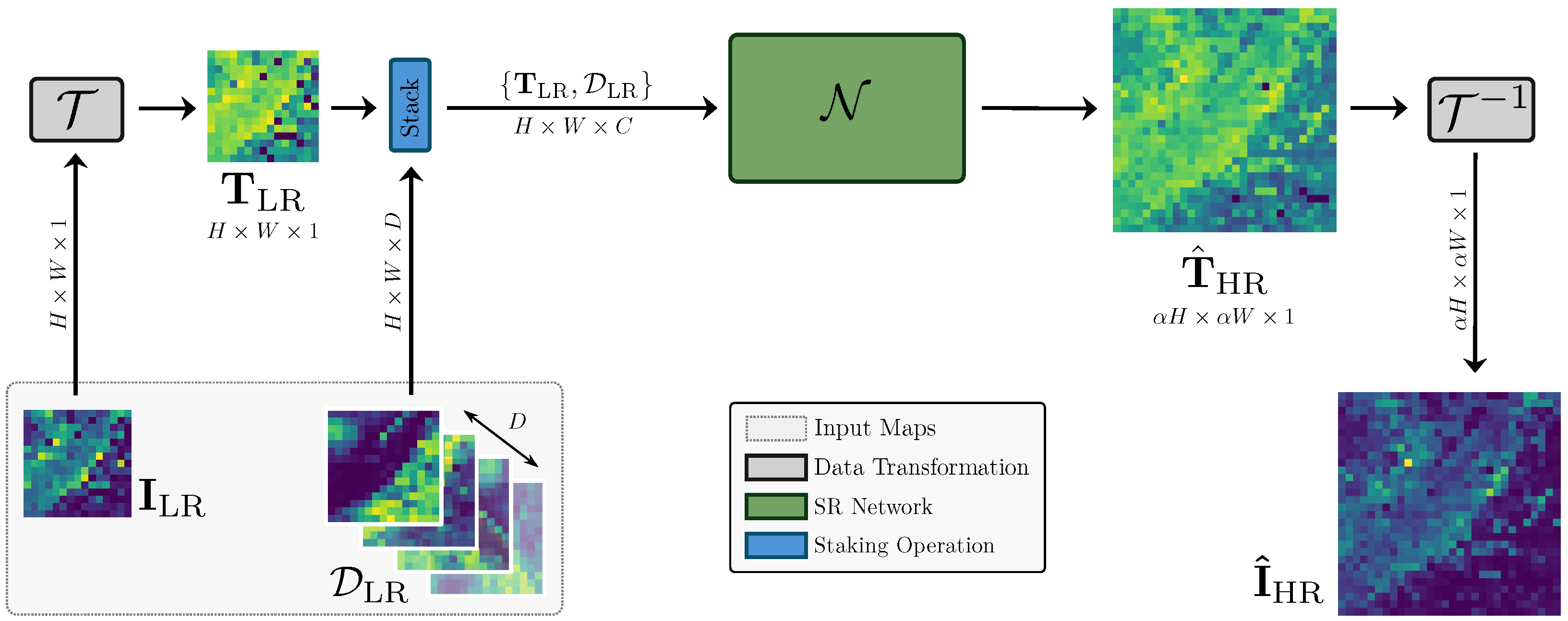
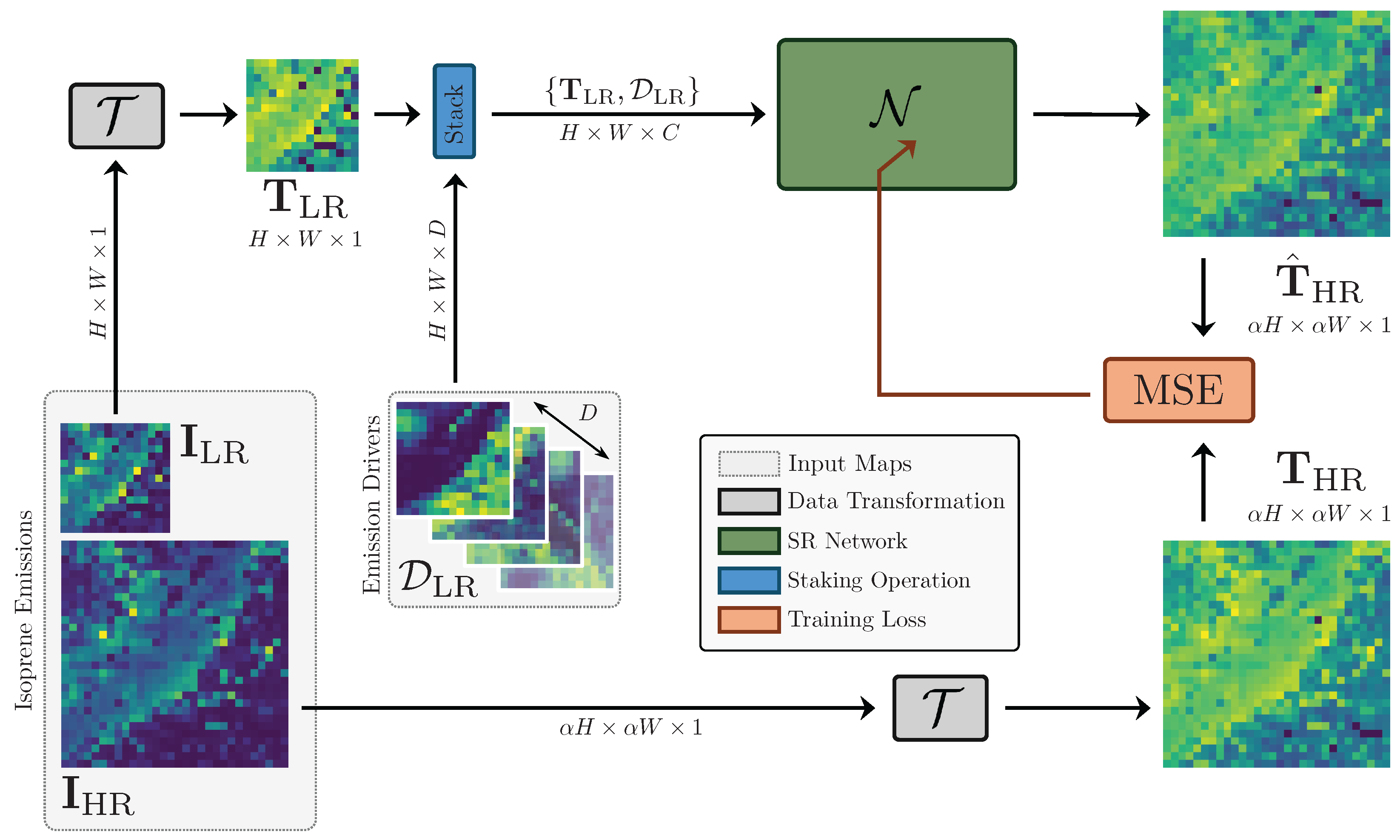
4.1. Leveraging Land Cover Priors for Isoprene Emission Super-Resolution

Accurate HR isoprene emission maps are critical for understanding BVOC dynamics and their environmental impacts. However, generating such maps at fine spatial resolutions remains challenging due to limitations in observational data and computational constraints in emission modeling. While traditional SISR methods can enhance LR emission maps using DL models [43,47,50,58], these approaches often rely solely on the inherent patterns within the LR input, neglecting ancillary environmental variables that drive emission processes [26,34,35].
In our prior work [50], we demonstrated the feasibility of applying SISR to isoprene emissions, reconstructing HR estimates from LR inputs using a DL-based SR network. However, this single-input formulation inherently limits the model’s ability to leverage domain-specific knowledge about the environmental drivers of isoprene emissions, such as LC characteristics. LC data encode critical ecological and environmental factors (e.g., vegetation type, canopy structure, and soil properties) that strongly influence biogenic emissions, as evidenced by extensive studies [24,25,74,75,77,78,79,80]. Integrating these drivers as auxiliary inputs could improve SR accuracy by grounding the reconstruction process in physically meaningful relationships [19,42,75,81].
In this work, we reformulate the problem as a MISR task, where an HR isoprene emission map is estimated by jointly leveraging (i) the LR isoprene emission map and (ii) multiple LR LC maps representing key emission drivers. This shift from SISR to MISR allows the model to exploit spatial and cross-feature correlations between isoprene emissions and LC variables, like vegetation type and urbanization levels.
We start considering the isoprene LR emission I LR that we want to super-resolve. Since isoprene emissions exhibit spatially sparse patterns and a wide dynamic range, we apply a non-linear transformation T ( · ) to the LR isoprene emission map, adopting the approach proposed in [50]. This transformation is derived from statistical analysis of the available HR data and is used to increase the robustness to outliers and local maxima, adapting the emission dynamics into more feasible values required for numerical stability when training Neural Networks (NNs). We define the transformed emissions as T HR and T LR for the HR and LR versions, respectively.
Then, we stack the transformed isoprene emission with D emission drivers, i.e., the LC maps. Specifically, the emission drivers are denoted with the set D LR = { D 1 , D 2 , , D D } . The selected emission drivers cover the same geographical area of the LR isoprene map they are stacked with. In stacking a single LR isoprene emission with D additional emission drivers, we obtain C = 1 + D emission maps, represented by the expression { T LR , D LR } .
We propose to estimate an HR isoprene emission map as
I ^ HR = T 1 ( N ( { T LR , D LR } ) ) ,
where N ( · ) is an NN architecture specifically designed for SR tasks. The operator T 1 ( · ) is the inverse transformation of T ( · ) , needed to re-adapt the super-resolved isoprene emissions to the BVOC dynamics [50].
Figure 1 depicts a sketch of the proposed methodology. We model the stacked set { T LR , D LR } as a tensor with a size of H × W × ( 1 + D ) , where H and W represent the height and width of the maps and D the number of emission drivers exploited in performing SR. The original I HR and the super-resolved emission I ^ HR have size α H × α W , with α > 1 indicating the SR factor, i.e., how much we increase the spatial resolution of the LR isoprene maps.
In the following, we provide details of the different modules that are included in our pipeline.

4.1.1. Isoprene Data Transformation

In our past investigations [50,66], we showed that a suitable data transformation is required to deal with biogenic emissions, i.e., isoprene, since they are characterized by sparsity, extremely small values, and wide dynamic ranges (from 10 18 to 10 3 [molec./cm2s] [68]). As a matter of fact, isoprene emissions can present many outliers due to the large spatial diversity of the environmental factors driving the emission process, such as meteorology, type of vegetation, seasonal cycle, and atmospheric composition [80,82]. For this reason, we adopt a non-parametric data transformation T ( · ) that forces emission values to follow a uniform distribution between 0 and 1 [50,83,84], enhancing robustness to outliers and local maxima, and at the same time, ensuring numerical stability during neural network training.

4.1.2. Super-Resolution Neural Networks

The choice of employing an NN as the SR operator N ( · ) is driven not only by the demonstrated superior performance of modern DL-based methods compared to traditional approaches but also by their inherent adaptability and flexibility. Specifically, in the context of MISR, DL-based solutions offer a significant advantage by eliminating the need to explicitly define a formal relationship between the various emission drivers, like LC information related to the geographic area to be super-resolved. This means that they can effectively capture the intricate dependencies between multiple diverse types of input images, thereby enhancing the overall performance and robustness of the SR task.
We investigate two NNs that are the state-of-the-art in SR, each leveraging advanced attention mechanisms: (i) the HAT [85], which combines transformer-based global attention [86] with local detail refinement; (ii) the Second-order Attention Network (SAN) [87], which utilizes second-order feature interactions to enhance the reconstruction of complex spatial patterns.
Both networks address the challenge of modeling long-range dependencies. HAT employs Residual Hybrid Attention Groups (RHAGs) for deep feature extraction, consisting of Hybrid Attention Blocks (HABs) and an Overlapping Cross-Attention Block (OCAB) [85]. HABs integrate Window-based Multi-head Self-Attention (W-MSA) and a Channel Attention Block (CAB), which utilizes channel attention, in parallel with a learnable weight [85]. To enhance cross-window interaction, HAT introduces OCABs [85] that use an Overlapping Cross-Attention (OCA) layer and a Multi-Layer Perceptron (MLP) layer. OCAs use overlapping window partitioning to effectively aggregate multi-scale contextual information by overlapping patches during attention computation. In contrast, SAN leverages a trainable Second-Order Channel Attention (SOCA) module, which learns channel inter-dependencies by exploiting second-order feature statistics through covariance normalization and global covariance pooling [87]. Furthermore, SAN incorporates Region-level Non-Local (RL-NL) modules [87] that divide the feature map into regions to capture long-distance spatial contextual information within these regions. The choice of these mechanisms could influence the network’s effectiveness in handling complex patterns and textures that span more significant emission map regions.
Notably, SAN has already been successfully applied to the SR of biogenic emissions [29,50,65,66]. Transformer-based SR networks for climate data are less explored in the literature, though the few existing applications show promising results [88].

4.2. Training Pipeline

We present the proposed training pipeline in Figure 2. We begin by considering the HR and its corresponding LR version of isoprene emissions, denoted as I HR and I LR , respectively. The selected D emission drivers from the D LR set are stacked with a transformed version of I LR , i.e., T LR = T ( I LR ) . Thus, after the stacking operation, we obtain a tensor { T LR , D LR } with dimensions H × W × C , where C = 1 + D .
This tensor is then fed into our SR network N , which outputs a super-resolved version of the isoprene map T ^ HR , with dimensions α H × α W × 1 , where α is the scale factor that represents the increase in spatial resolution.
We use the Mean Squared Error (MSE) as the loss function between the super-resolved map T ^ HR and the ground truth T HR = T ( I HR ) .

5. Experimental Dataset

5.1. Study Area

We select the European region as our study area, specifically focusing on the geographical extent defined by the TD-TROPO-010 isoprene inventory, i.e., 11.95°W, 44.95°E, 34.05°N, 71.95°N. Figure 3 provides a detailed illustration of the study area.

5.2. Pre-Processing Workflow

5.2.1. Land Cover Maps

We aim to super-resolve isoprene emission maps obtained from the TD-TROPO-010 inventory by exploiting LC information from the LC-ESA. As presented in Section 3.3, the LC-ESA dataset only captures a single temporal state (2021 snapshot), but since LC changes occur relatively slowly [75], it is assumed to be valid over the full observation period of TD-TROPO-010.
The LC-ESA dataset features 11 LC classes. We extract two different LC types relevant to biogenic emissions. Specifically, the CL and TC maps are selected since they represent two categories of underlying plant species whose biogenic emission mechanisms are essentially opposite in relation to isoprene emissions and thereby contain spatial patterns which are biologically relevant to isoprene emissions (common crops generally emit low amounts and trees generally higher amounts of isoprene) [22,23,35,75]. We later prove that they represent very informative biogenic emission drivers, as reported in Section 7.1. Instead of representing discrete classes (binary or categorical), we compute the proportion of each land type within the area represented by each grid cell. This transformation results in two distinct percentage maps, where each cell contains a continuous value between 0% and 100%. These maps provide a detailed view of the selected isoprene emission drivers, capturing mixed land uses within cells and enabling analysis of gradients, patterns, and changes while supporting SR models with continuous data.
After that, we spatially confine the two percentage maps from LC-ESA to the study area of the TD-TROPO-010. Due to the different spatial resolutions among the two datasets, a cell coordinate alignment process followed by spatial resolution matching is required. This is obtained by applying a coarsening function [89] over the entire map. After that, a bicubic interpolation function is used to align the resampled data to TD-TROPO-010 coordinates, ensuring that both datasets are consistently aligned, providing a congruous input of LC to isoprene emission data for SR model across the study area. Figure 4a,b report the CL and TC LC types, respectively, as percentages of the surface area underlying each grid cell over the full study area.

5.2.2. Leaf Area Index Maps

In addition to the LC maps, we also investigate the adoption of LAI information as an additional prior for the isoprene SR task. As reported in Section 3.2, the LAI-TROPO-010 inventory [71] provides the total leaf area per unit ground area. Similar to isoprene emissions, these maps cover Europe from 2018 to 2022, with a spatial resolution of 0.1 ° × 0.1 ° . In this inventory, LAI values range from 4.17 × 10 5 to 7.2 . Although LAI is defined as the ratio of the number of square meters of leaves per square meter of land surface, i.e., m 2 m 2 , values greater than one indicate that the area is covered with multiple layers of leaves, as in a forest canopy, where vegetation grows in layers above the ground. For instance, an LAI value of 5 conceptually represents five layers of leaves in that area. In Figure 4c, we report the monthly averaged LAI map (April 2019) over the entire study area.

5.2.3. Climate Class Maps

For a more reliable evaluation of the proposed methodology, we analyze the SR performance over the different Köppen–Geiger climate classes present in our study area. The climate classes are extracted from the CZ-KG-010 dataset. As presented in Section 3.4, the CZ-KG-010 dataset contains six different static maps, which differ in the years they cover. We adopt the map covering the 1991–2020 period, as this is the period of most significant overlap with the isoprene emissions in the TD-TROPO-010 inventory. We choose the native 0.1 ° × 0.1 ° resolution of the CZ-KG-010 to match the spatial resolution of the TD-TROPO-010 inventory. As previously conducted for the LC maps from the LC-ESA dataset, the coordinates of the climate class maps are aligned, and the spatial extent is reduced to match the study area set by the TD-TROPO-010 inventory. Figure 5 reports the geographical distribution of the Köppen–Geiger climate classes over the entire study area. In addition, Table 1 reports a detailed description for each climate class type [76].

5.3. Patch Extraction

Considering the TD-TROPO-010 inventory extension, we extract multiple HR patches from the entire maps with a 3 ° × 3 ° spatial coverage corresponding to 30 × 30 grid cells. Patches are created with a 1° stride to ensure continuous spatial coverage. Therefore, a 2° overlap in latitude and longitude over the study area is considered.
Following previous works on isoprene SR [50,65,66], a zero-thresholding criterion on isoprene emission patches is applied, promoting stability in the SR network training. Therefore, patches with more than 10% zero-value emission fluxes are discarded, as they provide insufficient isoprene information. This process results in a total number of 913,878 isoprene emission patches.
For an extensive experimental evaluation, patch-specific information, like the coordinates boundaries, daily time, and climate classes, are extracted, resulting in a complete dataset index that associates each patch with its specifications across the European extent of TD-TROPO-010.
From the HR isoprene emission maps and their associated emission drivers maps, we generate their LR counterpart by performing bicubic downsampling, obtaining maps of 15 × 15 grid cells. Our goal is to estimate HR isoprene emission patches I HR with 0.1 ° × 0.1 ° spatial resolution starting from their LR counterparts I LR and their related drivers in D LR , both having a 0.2 ° × 0.2 ° spatial resolution, thus addressing an SR scale factor α = 2 .
The extracted patches related to isoprene and its emission drivers form the complete experimental dataset. We denote the experimental dataset as S .

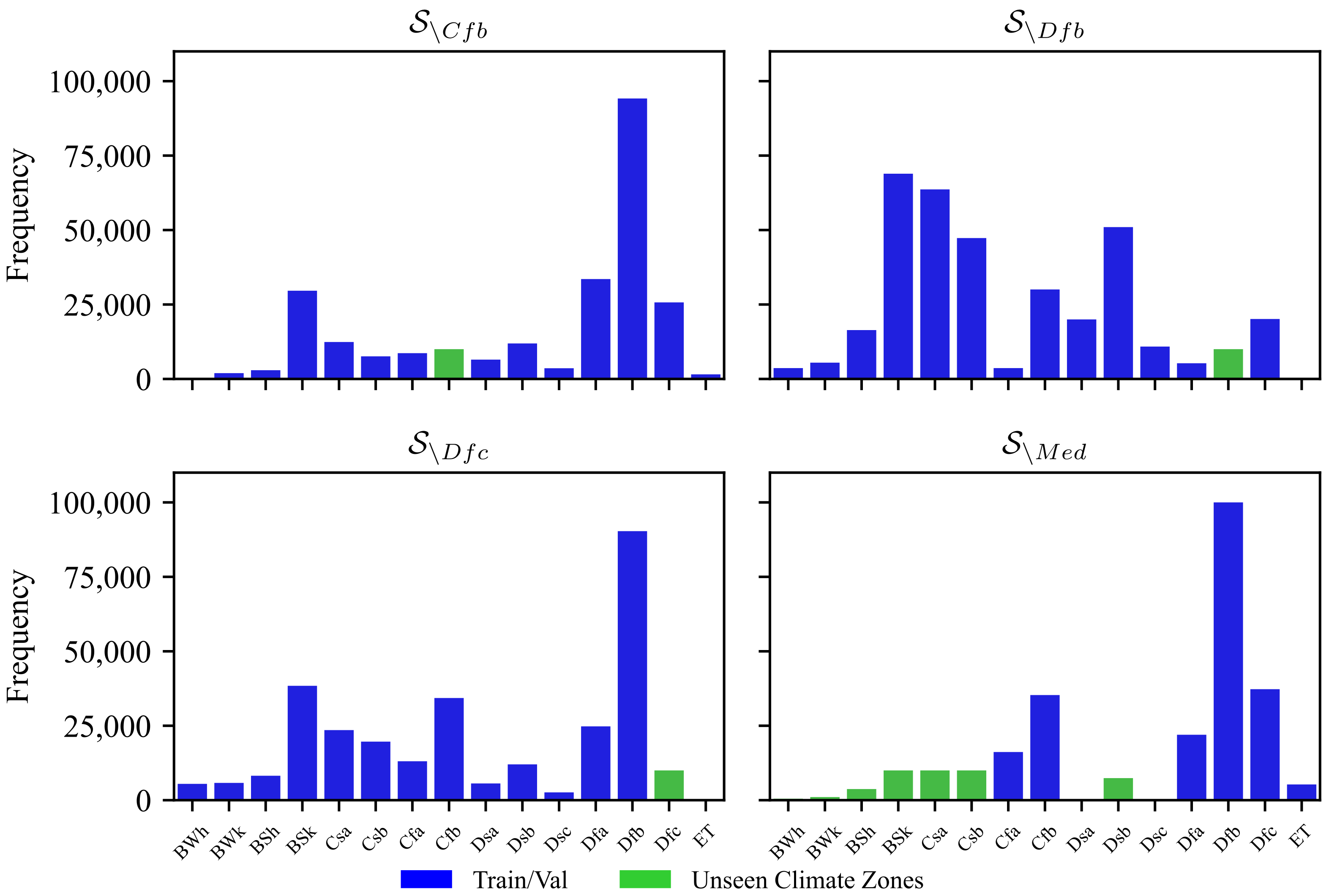
5.4. Climate-Specific Folding

Climate variability plays a crucial role in shaping isoprene emissions’ spatial and temporal distribution. Different climate zones exhibit distinct interactions between meteorological conditions, vegetation types, and emission drivers, making it challenging to develop a single model that generalizes well across all regions.
To address this, we adopt a specialized experimental strategy. From the entire experimental dataset S , we generate different folds covering the same temporal period, i.e., 2018–2022. Each fold, denoted as S \ c c , is structured around a specific climate class (cc) that is held out from the experimental data. Patches from the excluded climate class are treated as representing an unseen climate zone, enabling subsequent generalization experiments in Section 5.5.3.
Based on the distribution of climate classes across the study area, the three most frequently occurring classes, along with one custom Köppen–Geiger climate class, are selected as the held-out climate classes.
The selected classes are C f b , D f b , and D f c . In addition, we define a custom climate class M e d , where we include minor and sporadically occurring climate classes that are present in the Mediterranean area, making sure to reach a similar number of patches of the other climate classes. Creating a custom climate class was necessary because the geographical areas covered by the climate classes in M e d represent the study area under consideration. However, when taken individually, these classes do not contain sufficient patches to be considered a meaningful set for subsequent studies. For these reasons, we merged a subset of relevant climate classes for the study area to characterize it better.
Therefore, from the experimental dataset S , we generate four different folds, specifically { S \ C f b , S \ D f b , S \ D f c , S \ M e d } . Each fold excludes patches belonging to a selected climate class, i.e., C f b , D f b , D f c , and M e d .
Figure 6 reports the occurrences of the Köppen–Geiger climate classes over the study area. Colors denote which climate classes are considered for each of the four different dataset folds S \ c c .
In Figure 7 instead, we report the geographical distribution of the four climate-specific folds S \ c c .

5.5. Experimental Scenarios

To evaluate the capability of our proposed methodology, for each climate-specific fold S \ c c we analyze the model’s performance under three different scenarios:
  • Standard scenario, where training and evaluation data are coherent in terms of climate zones and geographical areas.
  • Unseen spatial areas scenario, in which we evaluate our method over geographical areas never seen in the training phase.
  • Unseen climate zone scenario, where we test over climate zones never seen in the training phase.
The purpose of these proposed scenarios is to compare and assess the model’s ability to super-resolve emissions with different environmental characteristics. In each scenario, experiments compare the models’ performance in the absence of emission drivers (i.e., using isoprene maps only) with the presence of emission drivers used as additional information for super-resolving isoprene maps. Below, we provide additional details and motivations for these experimental scenarios, highlighting their significance in addressing climate-specific challenges and improving the model’s generalization capabilities across diverse environmental conditions.

5.5.1. Standard Scenario

In this scenario, for each fold S \ c c , we randomly split the held-in patches using a 75 / 5 / 20 % strategy for the training, validation, and test partitions, respectively. In this way, the test partition contains patches that share the same geographical and climate coverage as the training and validation partitions. Referring to Figure 7, this scenario considers only patches randomly extracted from the blue areas for each climate fold.

5.5.2. Unseen Spatial Areas Scenario

This scenario focuses on investigating SR generalization across different geographical areas. This aspect is of great significance [11,14], especially given the comparatively strong performance of temporal generalization, as noted in previous studies on isoprene emission SR [50].
To achieve this, for each fold S \ c c , we create a spatial hold-out subset containing 10,000 patches from a specific area within the geographical extent of the climate-specific fold S \ c c . This spatial hold-out subset is then used as a test set for our model. Notice that the selected patches potentially include all the climate zones seen in the training phase, allowing the SR models to be tested on unseen spatial features while remaining within a familiar climate context. Figure 8 reports the geographical distribution of patches per fold. Specifically, the red area refers to the patches associated with the unseen spatial areas scenario.

5.5.3. Unseen Climate Zones Scenario

In this last scenario, we analyze the performance of our method by investigating the SR generalization across different climate conditions, testing the SR model on emission patches with unseen climate during training.
Since each fold S \ c c is structured in a way that a specific climate class (cc) is held out from the training data (see Section 5.4 for more details), some patches from that held-out climate class are selected as our test set. Specifically, for each fold S \ c c , 10,000 patches from the held-out climate class (cc) are randomly selected for testing. Figure 8 reports the geographical distribution of patches per fold. Specifically, green areas refer to patches associated with the unseen climate zone scenario.
The unseen areas and climate zone scenarios aim to ensure that each fold tests the performance of the SR model on distinct climate classes and geographical locations. Therefore, with this approach, we aim to capture most of the dataset’s variance to assess the SR performance accurately.

6. Experimental Setup

6.1. Training Settings

To estimate the data transformation T ( · ) , we follow the experimental setup proposed in [50]. To train the SR networks, we use the Adam optimizer with β 1 = 0.9 , β 2 = 0.99 , and an initial learning rate of 10 4 . We decrease the learning rate by a factor of 10 if the validation loss does not improve in 10 epochs until the minimum learning rate 10 7 is reached. We stop the learning phase if the validation loss does not improve after 50 epochs, setting a maximum number of epochs of 500.
In our experiments, we use an NVIDIA Titan V 12 GiB GPU (with 5120 CUDA cores at 1455 MHz) running on an Intel Xeon E5-2687W v4 CPU (with 48 Cores at 3 GHz) equipped with 252 GiB of RAM.
Kindly refer to the released implementation code for additional training and network details.

6.2. Evaluation Metrics

For a quantitative evaluation of the proposed method’s effectiveness, we conduct a comparison between the original HR isoprene emissions I HR and their super-resolved versions I ^ HR by adopting several metrics commonly used in the SR literature [4,88,90,91]. We evaluate our method in terms of Structural Similarity Index Measure (SSIM) [92], Peak Signal-to-Noise Ratio (PSNR), Universal Image Quality Index (UIQI) [93], Spatial Correlation Coefficient (SCC) [94]. In addition, we propose two additional metrics, the Normalized Mean Squared Error (NMSE) in dB and Maximum Absolute Error (MaxAE).
We define the NMSE as the ratio of the power of the error introduced by the SR process to the power of the original image and is defined as
NMSE ( I ^ HR , I HR ) = 10 log 10 MSE ( I ^ HR , I HR ) Avg ( I HR 2 )
where Avg extracts the mean value of the image.
The MaxAE quantifies the worst-case discrepancy between the super-resolved image I ^ HR and ground-truth I HR by identifying the maximum absolute difference at any pixel location of a 2D image, and it is defined as
MaxAE ( I ^ HR , I HR ) = max m , n I ^ HR ( m , n ) I HR ( m , n ) ,
where m and n denote the pixel coordinates of the considered emission map. Therefore, MaxAE measures the most significant error in the super-resolved image I ^ HR compared to the ground truth I HR .
The best values for these metrics are 1 for SSIM, UIQI, and SCC; the higher the better for PSNR; the less the better for NMSE and MaxAE.

7. Results

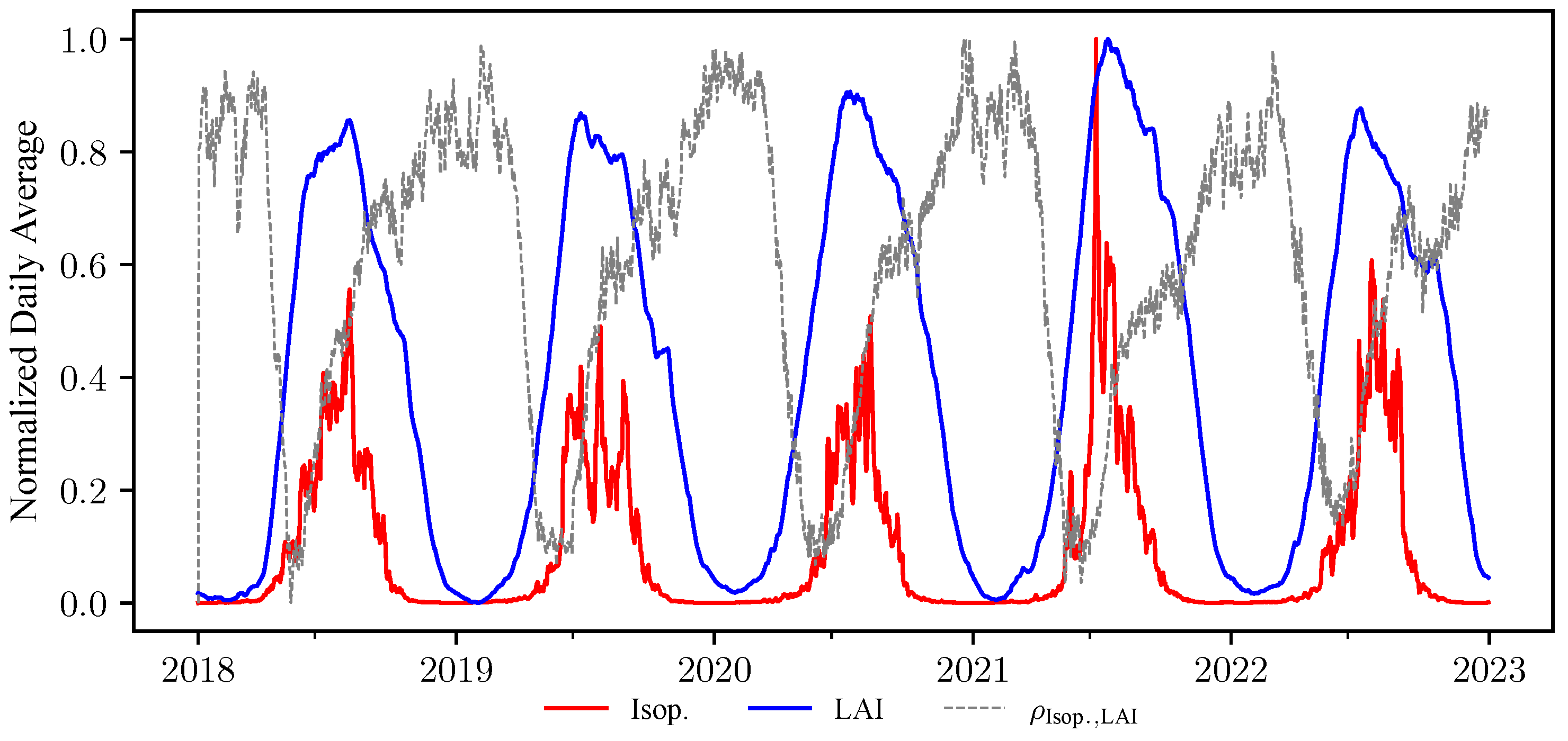
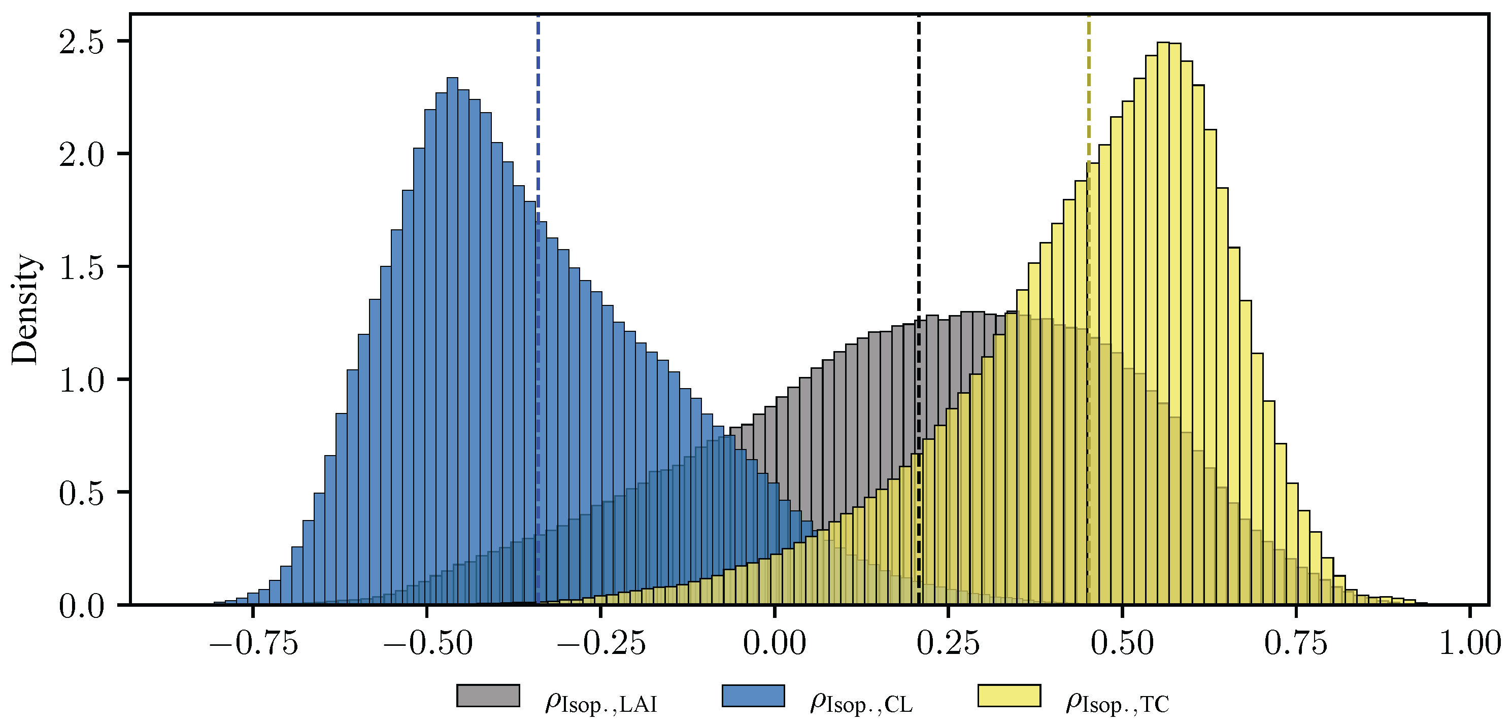
7.1. Selecting the Emission Drivers

In this section, we conduct a comprehensive statistical analysis to evaluate the strength and significance of the relationships between isoprene emissions and the Leaf Area Index (LAI), Cropland (CL), and Tree Cover (TC) information. This analysis aims to identify which of these drivers has the most substantial influence on isoprene emissions, providing insights into the key factors governing these emissions. To assess the relationships across the temporal and spatial extent of the TD-TROPO-010 inventory, we use the Pearson Correlation Coefficient (PCC) and the entropy, denoted with H .
We start by analyzing the temporal dependencies of isoprene emissions and LAI information. LAI patches from the LAI-TROPO-010 inventory are extracted following the same operations conducted for isoprene, explained in Section 5.3, and have the same geographical extent as our study area. Figure 9 reports their temporal evolution, considering the mean values of patches, together with the evolution of their PCC. Although LAI mean intensities follow a seasonal cycle similar to that of isoprene emissions, the correlation between isoprene (isop.) emissions and LAI values (i.e., ρ isop . , LAI ) varies significantly over time. Interestingly, this temporal correlation displays a cyclical pattern offset by half a year from the seasonal cycles of both variables. Specifically, the correlation peaks are in the winter months, when both LAI and isoprene emission intensities are at their lowest. This finding highlights that the LAI on its own might not be a robust indicator for structures within isoprene emission patterns, as was already pointed out in [95]. Given these results, we believe that the LAI does not represent a suitable driver for the spatial patterns underlying isoprene emission imagery, particularly during periods of high biological activity.
In addition, we analyze the spatial correlation of isoprene emissions with LAI, CL, and TC information. In Figure 10, we report the results of this analysis. The correlation between isoprene emission and LAI ( ρ isop . , LAI ) is widely distributed (the standard deviation σ = 0.29 ) with a low average value of μ = 0.21 . In contrast, the correlation with CL data exhibits a narrower distribution ( σ = 0.20 ) with a negative μ = 0.34 . Lastly, the TC correlation also shows a relatively narrow distribution ( σ = 0.21 ) but has the highest value μ = 0.45 . Given these results, the TC information seems the most suitable candidate out of the three for augmenting isoprene emissions in SR applications.
However, as found in previous works [29,31], we believe that information with inherent negative spatial correlation could be helpful in spatially enhancing isoprene emission maps, suggesting that CL data may also be a valuable prior for SR purposes. Since the aim is to establish a consistent relationship from additional channels (drivers) to support SR, the temporally static nature of LC data (single 2021 snapshot [73]) with a relatively narrow distribution of patch correlations makes CL and TC data potentially suitable for this purpose.
Further investigations into the statistical relationships between patches reveal that the entropy of isoprene emission patches conditioned to LC data, i.e., H ( isop . | CL ) and H ( isop . | TC ) , are higher and more narrowly distributed than that conditioned to LAI, i.e., H ( isop . | LAI ) , as illustrated in Figure 11. Among LC types, TC information leads to the highest average ( μ = 3.68 ), while CL data have a slightly higher median value ( M = 3.83 ) compared to TC ( M = 3.79 ). Assuming that higher conditional entropy indicates more significant potential for improving SR learning, these findings suggest that both TC and CL data could contribute to enhanced SR performance.

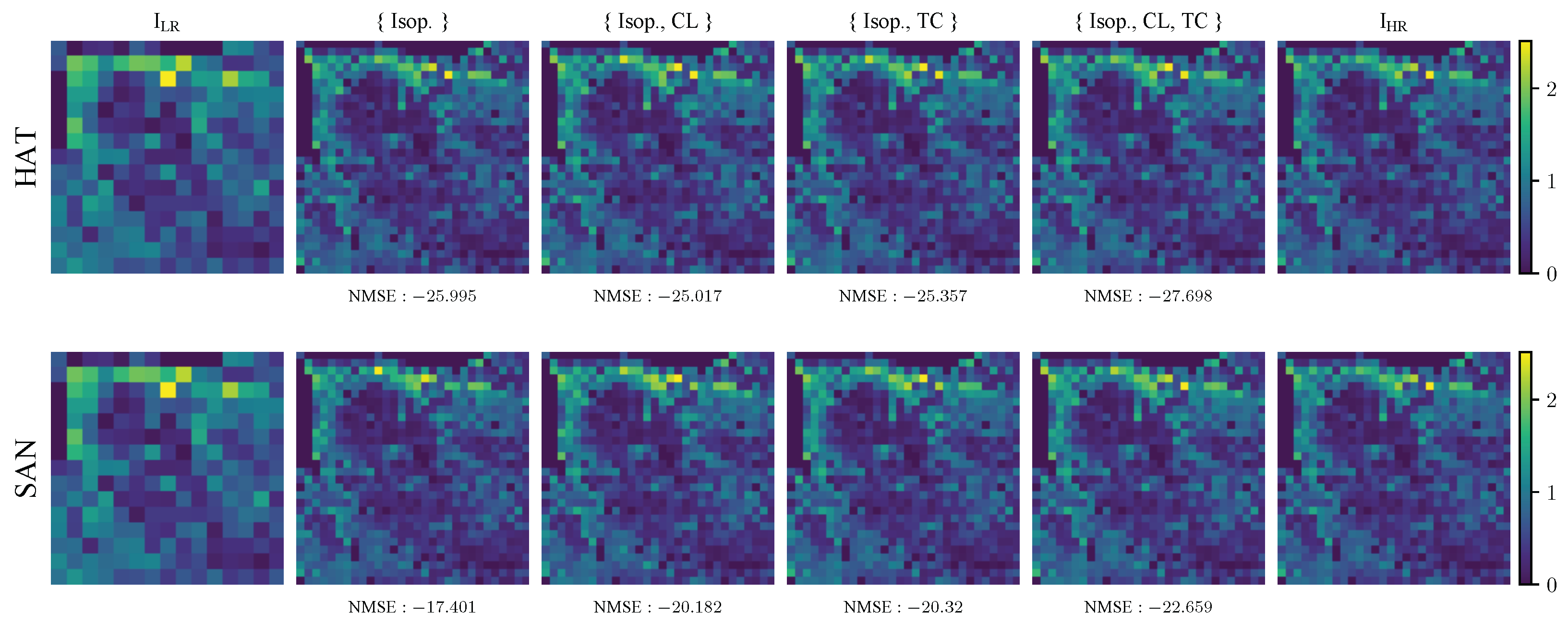
7.2. Leveraging Semantic Priors

In this section, we evaluate the effectiveness of our proposed methodology in integrating semantic information from LC data as emission drivers to enhance the spatial resolution of isoprene emission maps.
For a more detailed analysis, we assess the performance of our proposed methodology by training a separate system for each of the four class-specific dataset folds S \ c c . This results in four distinct training instances, each excluding patches from a specific climate class while maintaining the same system architecture (see Section 5.5.1 for more details). We start evaluating results by using patches from the test partition of the standard scenario reported in Section 5.5.1.
We use our previous approach proposed in [50] as a baseline. In this approach, the HR isoprene emission map is estimated solely from its corresponding LR version, without incorporating any additional emission drivers to guide the SR process. Therefore, the super-resolved isoprene map is computed as
I ^ HR = T 1 ( N ( T LR ) ) .
Transformed data domain. To simplify, we start performing an analysis in the transformed data domain, considering emissions after the application of the data transformation, i.e., directly comparing the HR transformed emission T HR = T ( I HR ) and the output of the SR network T ^ HR . We compare the performance by computing the Normalized Improvement Ratio (NIR), defined as
NIR ( T HR , T ^ HR , T ^ HR Ref . ) = NMSE ( T ^ HR , T HR ) NMSE ( T ^ HR Ref . , T HR ) NMSE ( T ^ HR Ref . , T HR ) ,
where T ^ HR Ref . = N ( T LR ) is the super-resolved isoprene emission estimated by our baseline method [50], thus using only the LR isoprene emission I LR as input without considering any additional emission drivers D LR . Instead, T ^ HR is the super-resolved emission obtained using our proposed methodology, exploiting information from additional LC data.
In Figure 12, we report the result of this study for both the considered SR networks, i.e., SAN and HAT.
For the SAN, the 3-channel configuration (i.e., { Isop . , CL , TC } ) consistently outperforms the other setups across all folds. The 2-channel experiments with CL data ( { Isop . , CL } ) show improved performance. In contrast, the 2-channel experiments with TC data ( { Isop . , TC } ) vary significantly, showing benefits in two of the four folds but lacking consistency overall.
The HAT model shows a different pattern: 2-channel configurations generally decrease performance, while 3-channel configurations show stable and consistent improvements across folds. The most varying case is encountered in the M e d fold, i.e., S \ M e d , where the 2-channel CL and TC cases yield opposite trends for both SAN and HAT models, but the 3-channel cases both improve their performance.
These findings reflect that performance characteristics of different DL architectures may vary significantly on the same data. Specifically, the negatively correlated CL data benefit the SAN model. In contrast, the same data detract from HAT’s performance concerning the single channel reference. Overall, the 3-channel experiments benefit, in all cases, from including the additional structural information shown in the LC maps.
Isoprene data domain. We now perform an analysis on the isoprene data domain, thus considering emissions after the back transformation of the SR output in the isoprene data range, i.e., I ^ HR = T 1 ( T ^ HR ) .
In Figure 13, we report the NMSE, considering isoprene emissions for each fold. Comparing the results before (upper distribution, using T ^ HR ) and after applying the inverse data transformation (bottom distribution, using I ^ HR ), we can notice a marked drop in performance. This drop occurs for both networks in all folds and across all configurations. We believe it is due to the non-linear mapping introduced by the data transformation T ( · ) and its inverse T 1 ( · ) . Although the improvements concerning the isoprene-only scenario (1-channel, { Isop . } ) remain consistent in their trends, a performance deterioration can be observed for both the SR networks if compared to the transformed domain.
In Figure 14, we report a super-resolved emission example I ^ HR taken from the S \ C f b fold from both the SR networks and considering all the input configurations. In addition to the super-resolved emission I ^ HR , we include its related I LR (first column, input) and I HR (last column, ground-truth) emissions. Notice that the three-channel configuration reports the best reconstruction results, in terms of NMSE.
Complete metrics analysis. For a complete analysis of all the metrics, we report the NMSE, SSIM, PSNR, MaxAE, UIQI, and SCC for all the considered configurations, before ( T ^ HR ) and after ( I ^ HR ) the application of the inverse data transformation in Table 2 and Table 3, respectively.
We can observe that HAT significantly outperforms SAN. Additionally, except for S \ M e d , the { Isop . , CL , TC } configuration performs best, while the second-best is the baseline configuration, i.e., { Isop . } . However, for S \ M e d , the best-performing configuration is the 2-channel { Isop . , TC } , followed by the 3-channel configuration, i.e., { Isop . , CL , TC } .
Across all input configurations, HAT demonstrates more stable performance than SAN, as evidenced by lower standard deviations in metrics like SSIM and higher consistency in MaxAE and UIQI across data folds. This stability can be attributed to their distinct attention mechanisms. SAN, which leverages second-order channel attention, is more sensitive to high-frequency components. While this enhances fine details, it also amplifies noise when handling unseen data.
These results are consistent both before (Table 2, using T ^ HR ) and after (Table 3, using I ^ HR ) applying the inverse data transformation.
Moreover, in Table 4, we report the training times and epochs required for convergence for each experiment. It is worth noting that adding additional information, such as emission drivers in D LR , often increases the complexity of the model. Although additional inputs can provide physically relevant constraints that, in theory, help regularize the learning process and reduce the inherent ill-posedness of the SR problem, this benefit is not always observed in practice. Indeed, the increased complexity typically leads to longer runtimes and more epochs needed to reach convergence. However, the 2-channel configurations, i.e., { Isop . , CL } and { Isop . , TC } , are generally faster than both the 1-channel, i.e., { Isop . } , and 3-channel, i.e., { Isop . , CL , TC } configurations for both SR networks, likely due to a better balance between information richness and computational overhead.
The transformer-based HAT network, due to its higher computational complexity, requires more epochs and longer training times than the SAN network. Its convergence depends on the data fold used, as different climate zones exhibit varying emission patterns. Regions with complex emissions may need more epochs, while uniform areas converge faster. This highlights the importance of diverse training data. While additional inputs offer physical constraints, they also increase model complexity, requiring a careful balance between input information, computational cost, and convergence efficiency.

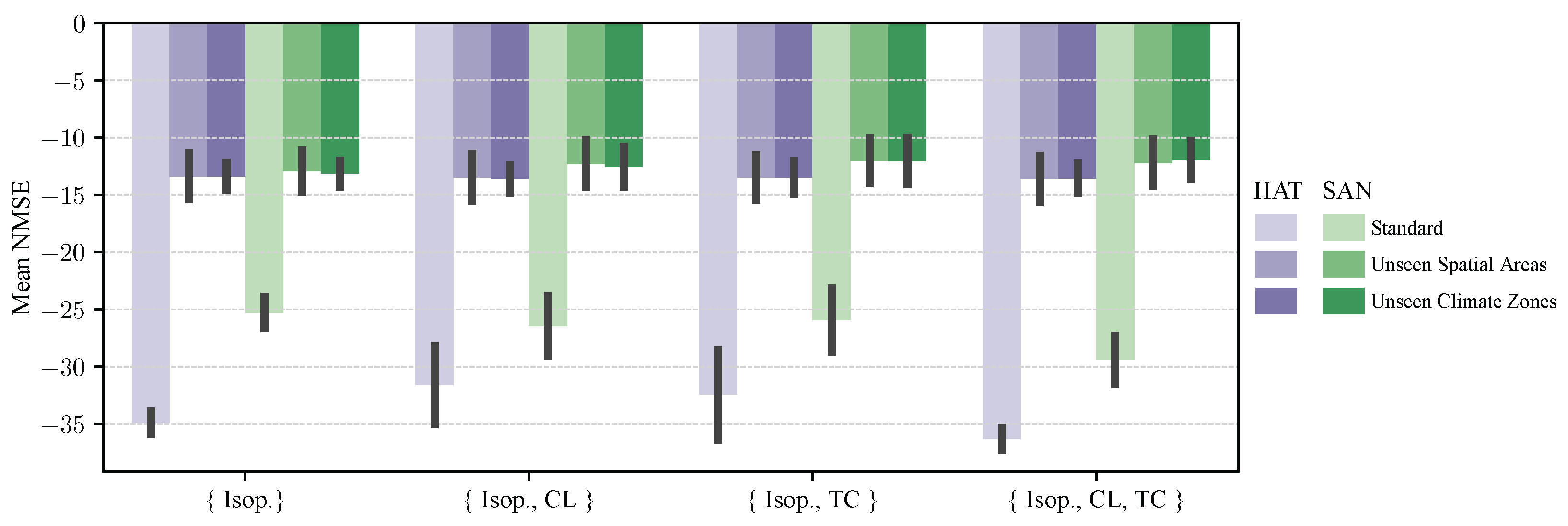
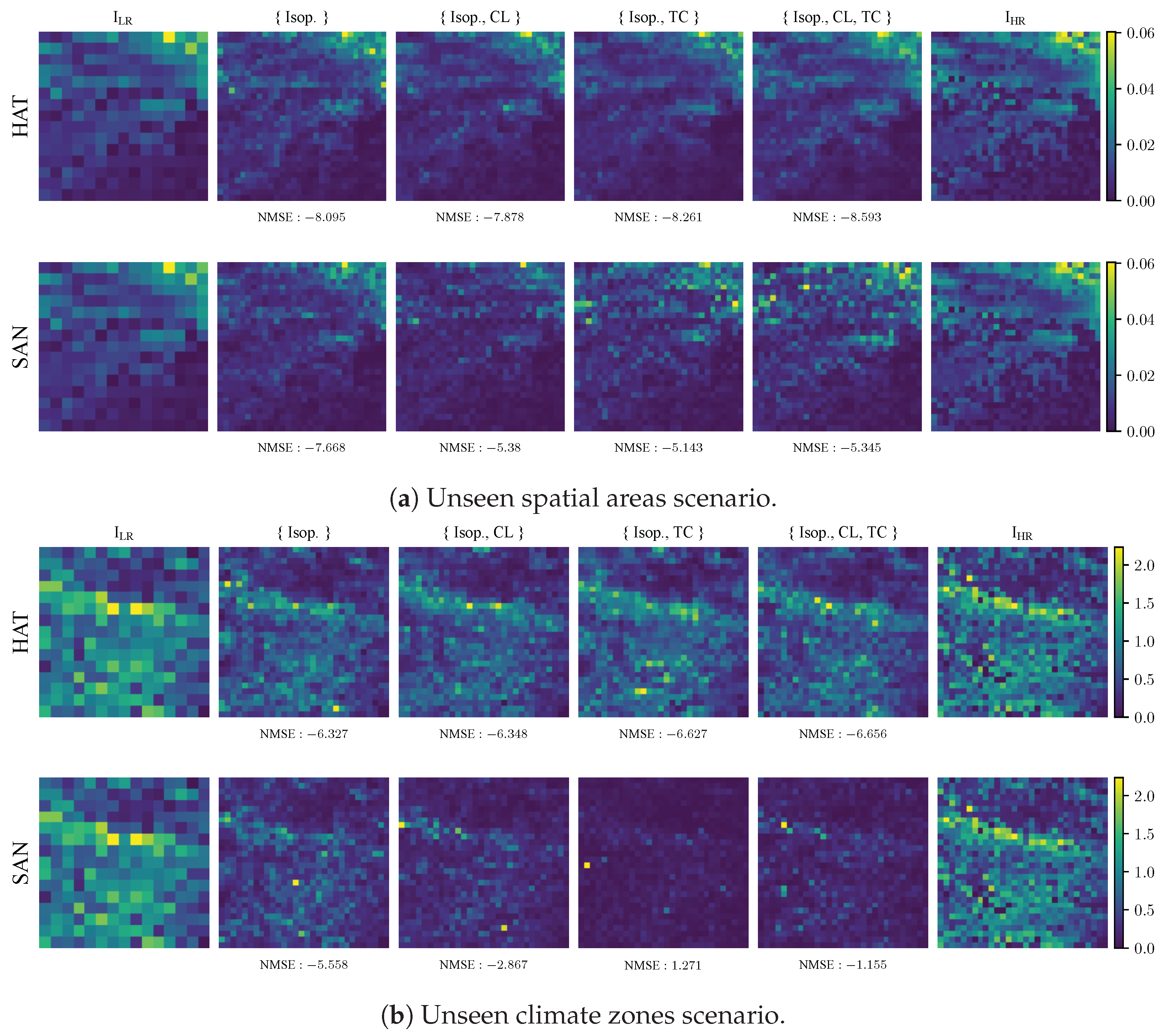
7.3. Generalization Studies

To assess the model capabilities in super-resolving unseen emissions during training, we perform generalization studies addressing the two additional scenarios presented in Section 5.5: (i) the unseen spatial areas scenario; (ii) the unseen climate zones scenario. We perform these investigations for each S \ c c fold of the entire experimental dataset S .
For the unseen spatial areas scenario (Section 5.5.2), isoprene emissions from a specific geographical region with the same climate classes as the training data are used in the test phase. This is conducted to assess the model’s ability to generalize to different geographical areas while keeping climate conditions consistent with those seen during training.
Regarding the unseen climate zones scenario (Section 5.5.3), the test emissions refer exclusively to a specific climate class not used in training, forcing the model to super-resolve emissions from an unseen climate zone.
Figure 15 reports the result obtained using the SAN and the HAT networks, averaged across the four S \ c c folds. We also show the test set performance when considering the standard scenario (Section 5.5.1). The reported NMSE is referred to the transformed data domain, thus assessing the SR performance on the T ^ HR isoprene emissions.
We can notice a significant performance drop in both the unseen spatial and climate sets compared to the standard test set. This demonstrates the models’ challenges when generalizing to unseen contexts. Moreover, including additional priors to guide the SR process is not helpful in either unseen set.
In Figure 16, we report SR examples to highlight the different behaviors adopted by our SR networks when dealing with unseen emissions. We can notice subtle differences in reconstructing emission patterns by looking at the four super-resolved versions I ^ HR . Specifically, SAN leads to noisier and inaccurate emission patterns in the super-resolved outputs. In contrast, HAT integrates multiple attention mechanisms, providing implicit regularization that results in smoother and more stable reconstructions.
It is worth noticing that, even if the achieved NMSE values are significantly lower than in the standard scenario, HAT always carries more accurate SR than SAN. We conjecture that the more substantial feature aggregation in HAT helps suppress noise and improves robustness when generalizing to novel patterns, as reflected in its superior performance across all configurations.

8. Discussion

This study has shown the potential of leveraging Land Cover (LC) priors to enhance the spatial resolution of isoprene emission maps over Europe using DL-based SR techniques. By incorporating Cropland (CL) and Tree Cover (TC) data, we can augment isoprene emission predictions, providing insights into the interplay between land use characteristics and BVOC dynamics.
The statistical analysis in Section 7.1 revealed that TC exhibited the strongest correlation with isoprene emissions, while CL showed a moderate, albeit negative, correlation. These findings underscore the importance of vegetation type and density in determining isoprene emissions, as TC acts as a significant source of isoprene. Interestingly, while the Leaf Area Index (LAI) captures seasonal variations in vegetation, its weak spatial correlation with isoprene emissions suggested it is less effective as a direct driver for spatial SR tasks. However, the inclusion of LAI may still be beneficial for capturing temporal dynamics in future models.
The comparison of SISR and MISR approaches highlighted the advantages of incorporating multiple drivers into the SR process. Specifically, the HAT and SAN models both exhibited improved performance when CL and TC data are included, as we can see from Figure 12. Among the configurations tested, the 3-channel approach, i.e., including CL and TC information in the SR process, consistently outperformed single-channel and 2-channel setups, demonstrating the value of integrating diverse data sources to enhance spatial predictions.
While the 3-channel experiments did not converge in fewer epochs than the 1- and 2-channel setups, they achieved significantly higher reconstruction accuracy. This improvement can be attributed to the additional channels providing richer semantic priors, which better constrain the ill-posed nature of the SR problem. This finding highlights the importance of leveraging diverse, complementary data sources to enhance the precision of the SR process, even if computational efficiency remains comparable.
The observed differences in performance between the HAT and SAN models can be attributed to their architectural designs. HAT, leveraging transformer-based global attention mechanisms, excels in capturing long-range dependencies and large-scale spatial patterns, making it particularly suitable for scenarios where broader geographic or environmental contexts influence emission patterns. In contrast, SAN’s second-order attention mechanism is adept at modeling localized and fine-grained spatial details, providing an advantage in regions with high emission variability or complex local patterns. These complementary strengths highlight the importance of selecting architectures based on the specific characteristics of the data and the target application.
The generalization studies, which evaluated the models’ performance on unseen climate zones and geographic regions, revealed a significant drop in performance compared to the standard test set. Several factors may explain this. First, the training dataset likely underrepresents certain climate zones or geographic regions, limiting the model’s ability to learn robust patterns applicable to diverse contexts. Second, isoprene emissions are highly dynamic and influenced by complex environmental factors, making extrapolation to unseen conditions challenging.
Additionally, the reliance on static LC data may introduce temporal inconsistencies. As a matter of fact, the LC maps represent a snapshot in time and do not account for seasonal or long-term changes in vegetation, potentially leading to misalignment with the isoprene emission dynamics in unseen regions. This temporal mismatch underscores the need for integrating dynamic priors, such as real-time vegetation indices or meteorological variables, to improve generalization performance.
Finally, the high sparsity and variability of isoprene emissions further complicate the learning process. Sparse data, particularly in regions with low emission levels, may hinder the models’ ability to generalize effectively to areas with distinct emission characteristics.
Future research should focus on integrating dynamic datasets, such as time-varying vegetation indices, climate-related variables, and biophysical and deposition products, to capture temporal variations in isoprene emissions better. Exploring hybrid architectures that combine the strengths of HAT and SAN could further enhance model performance across diverse regions. Further work should also quantify the impact of training hyperparameters on the robustness and optimization potential of the results. Additionally, since biases introduced during the derivation of isoprene emission inventories may propagate into the DL system, expanding the scope of the study to include available isoprene emission maps derived with different methods (e.g., SEEDS bottom-up isoprene emissions [96]), or incorporating DA techniques [66], would allow further investigation of the broader applicability of our proposed method. Also, utilizing global datasets, multi-year observations, and different SR-Factors (e.g., α = 4 , or α = 8 ) would enable a more comprehensive evaluation of the model’s scalability and generalization capabilities.

9. Conclusions

This study explored the integration of Land Cover (LC) priors into DL-based SR frameworks to enhance the spatial resolution of isoprene emission maps. By incorporating Cropland (CL) and Tree Cover (TC) data as emission drivers, we demonstrated significant improvements in the accuracy of super-resolved isoprene maps. Notably, we utilized the most up-to-date and high-resolution isoprene inventory over Europe, further enhancing the precision and validity of our results. The findings highlight the critical role of vegetation types in influencing BVOC emissions and underscore the potential of MISR techniques for addressing spatial resolution challenges in atmospheric research.
The 3-channel experiment consistently outperformed other configurations. Including additional semantic priors constrained the ill-posed nature of the SR problem, highlighting the value of integrating diverse data sources to guide SR processes.
The comparison between the HAT and SAN models revealed distinct strengths in capturing global versus localized emission patterns, emphasizing the importance of architecture selection based on data characteristics. However, the generalization studies underscored key challenges, including the difficulty of extrapolating to unseen climate zones and geographic regions and the limitations of relying on static LC data.
Despite these challenges, the proposed approach provides a valuable foundation for improving BVOC emission inventories, with implications for air quality monitoring, climate modeling, and ecological research. Future work should focus on integrating dynamic and diverse datasets, developing hybrid architectures, investigating generative SR-frameworks such as GANs [62] and diffusion models [63], and expanding the geographical and temporal scope of the study. To validate future advances in isoprene super-resolution, additional studies should also focus on measurable impacts on downstream systems such as improvements in air quality forecasting. These efforts will be crucial for advancing the scalability and applicability of SR methods in atmospheric and climate sciences.

Author Contributions

Conceptualization, C.U., A.G. and S.M.; methodology, C.U., A.G. and S.M.; software, C.U. and A.G.; validation, C.U., A.G. and S.M.; formal analysis, C.U., A.G. and S.M.; investigation, C.U. and A.G.; resources, C.U. and A.G.; data curation, C.U.; writing—original draft preparation, C.U., A.G. and S.M.; writing—review and editing, C.U., A.G., S.M. and P.B.; visualization, C.U. and A.G.; supervision, A.G., S.M., P.B. and S.T.; project administration, S.T. All authors have read and agreed to the published version of the manuscript.

Funding

This research received no external funding.

Data Availability Statement

The implementation code of the presented methodology is available at https://github.com/polimi-ispl/sr-bvoc-lc (accessed on 14 March 2025). The TD-TROPO-010 isoprene emission inventory is available at https://www.seedsproject.eu/data/top-down-isoprene-emissions (accessed on 14 March 2025). The LAI-TROPO-010 inventory is available at https://www.seedsproject.eu/data/lai-ol (accessed on 14 March 2025). The LC-ESA inventory is available at https://zenodo.org/records/7254221 (accessed on 14 March 2025). The CZ-KG-010 inventory is available at https://www.gloh2o.org/koppen/ (accessed on 14 March 2025). No restrictions apply to the availability of these data.

Acknowledgments

This work was supported by the Italian Ministry of University and Research (MUR) and the European Union (EU) under the PON/REACT project.

Conflicts of Interest

The authors declare no conflicts of interest.

References

  1. Chen, C.H. (Ed.) Signal and Image Processing for Remote Sensing, 3rd ed.; Signal and Image Processing of Earth Observations; CRC Press: Boca Raton, FL, USA, 2024. [Google Scholar]
  2. Tuia, D.; Schindler, K.; Demir, B.; Zhu, X.X.; Kochupillai, M.; Džeroski, S.; van Rijn, J.N.; Hoos, H.H.; Del Frate, F.; Datcu, M.; et al. Artificial Intelligence to Advance Earth Observation: A review of models, recent trends, and pathways forward. IEEE Geosci. Remote Sens. Mag. 2024, 2–25. [Google Scholar] [CrossRef]
  3. Reichstein, M.; Camps-Valls, G.; Stevens, B.; Jung, M.; Denzler, J.; Carvalhais, N.; Prabhat. Deep learning and process understanding for data-driven Earth system science. Nature 2019, 566, 195–204. [Google Scholar] [CrossRef] [PubMed]
  4. Sdraka, M.; Papoutsis, I.; Psomas, B.; Vlachos, K.; Ioannidis, K.; Karantzalos, K.; Gialampoukidis, I.; Vrochidis, S. Deep Learning for Downscaling Remote Sensing Images: Fusion and super-resolution. IEEE Geosci. Remote Sens. Mag. 2022, 10, 202–255. [Google Scholar] [CrossRef]
  5. Siddique, M.A.; Naseer, E.; Usama, M.; Basit, A. Estimation of Surface-Level NO2 Using Satellite Remote Sensing and Machine Learning: A review. IEEE Geosci. Remote Sens. Mag. 2024, 12, 8–34. [Google Scholar] [CrossRef]
  6. Hobeichi, S.; Nishant, N.; Shao, Y.; Abramowitz, G.; Pitman, A.; Sherwood, S.; Bishop, C.; Green, S. Using Machine Learning to Cut the Cost of Dynamical Downscaling. Earth’s Future 2023, 11, e2022EF003291. [Google Scholar] [CrossRef]
  7. Rampal, N.; Hobeichi, S.; Gibson, P.B.; Baño-Medina, J.; Abramowitz, G.; Beucler, T.; González-Abad, J.; Chapman, W.; Harder, P.; Gutiérrez, J.M. Enhancing Regional Climate Downscaling through Advances in Machine Learning. Artif. Intell. Earth Syst. 2024, 3, 230066. [Google Scholar] [CrossRef]
  8. Sokhi, R.S.; Moussiopoulos, N.; Baklanov, A.; Bartzis, J.; Coll, I.; Finardi, S.; Friedrich, R.; Geels, C.; Grönholm, T.; Halenka, T.; et al. Advances in air quality research—Current and emerging challenges. Atmos. Chem. Phys. 2022, 22, 4615–4703. [Google Scholar] [CrossRef]
  9. Park, S.; Singh, K.; Nellikkattil, A.; Zeller, E.; Mai, T.; Cha, M. Downscaling Earth System Models with Deep Learning. In Proceedings of the ACM SIGKDD Conference on Knowledge Discovery and Data Mining, Washington, DC, USA, 14–18 August 2022; pp. 3733–3742. [Google Scholar]
  10. Baño Medina, J.; Manzanas, R.; Cimadevilla, E.; Fernández, J.; González-Abad, J.; Cofiño, A.S.; Gutiérrez, J.M. Downscaling multi-model climate projection ensembles with deep learning (DeepESD): Contribution to CORDEX EUR-44. Geosci. Model Dev. 2022, 15, 6747–6758. [Google Scholar] [CrossRef]
  11. Baño-Medina, J.; Iturbide, M.; Fernández, J.; Gutiérrez, J.M. Transferability and Explainability of Deep Learning Emulators for Regional Climate Model Projections: Perspectives for Future Applications. Artif. Intell. Earth Syst. 2024, 3, e230099. [Google Scholar] [CrossRef]
  12. Chiang, C.H.; Huang, Z.H.; Liu, L.; Liang, H.C.; Wang, Y.C.; Tseng, W.L.; Wang, C.; Chen, C.T.; Wang, K.C. Climate Downscaling: A Deep-Learning Based Super-resolution Model of Precipitation Data with Attention Block and Skip Connections; National Taiwan Normal University: Taiwan, China, 2023. [Google Scholar]
  13. Wang, M.; Franklin, M.; Li, L. Generating Fine-Scale Aerosol Data through Downscaling with an Artificial Neural Network Enhanced with Transfer Learning. Atmosphere 2022, 13, 255. [Google Scholar] [CrossRef]
  14. Yadav, N.; Sorek-Hamer, M.; Von Pohle, M.; Asanjan, A.A.; Sahasrabhojanee, A.; Suel, E.; Arku, R.E.; Lingenfelter, V.; Brauer, M.; Ezzati, M.; et al. Using deep transfer learning and satellite imagery to estimate urban air quality in data-poor regions. Environ. Pollut. 2024, 342, 122914. [Google Scholar] [CrossRef] [PubMed]
  15. Geiss, A.; Silva, S.J.; Hardin, J.C. Downscaling atmospheric chemistry simulations with physically consistent deep learning. Geosci. Model Dev. 2022, 15, 6677–6694. [Google Scholar] [CrossRef]
  16. Liu, Y.; Qiao, Y.; Hao, Y.; Wang, F.; Rashid, S.F. Single Image Super Resolution Techniques Based on Deep Learning: Status, Applications and Future Directions. J. Image Graph. 2021, 9, 74–86. [Google Scholar] [CrossRef]
  17. Eyring, V.; Collins, W.D.; Gentine, P.; Barnes, E.A.; Barreiro, M.; Beucler, T.; Bocquet, M.; Bretherton, C.S.; Christensen, H.M.; Dagon, K.; et al. Pushing the frontiers in climate modelling and analysis with machine learning. Nat. Clim. Change 2024, 14, 916–928. [Google Scholar] [CrossRef]
  18. Materia, S.; García, L.P.; van Straaten, C.; O, S.; Mamalakis, A.; Cavicchia, L.; Coumou, D.; de Luca, P.; Kretschmer, M.; Donat, M. Artificial intelligence for climate prediction of extremes: State of the art, challenges, and future perspectives. WIREs Clim. Change 2024, 15, e914. [Google Scholar] [CrossRef]
  19. Do, T.N.N.; Sudo, K.; Ito, A.; Emmons, L.; Naik, V.; Tsigaridis, K.; Seland, Ø.; Folberth, G.A.; Kelley, D.I. Historical Trends and Controlling Factors of Isoprene Emissions in CMIP6 Earth System Models. EGUsphere 2024, 2024, 1–49. [Google Scholar] [CrossRef]
  20. Weber, J.; Archer-Nicholls, S.; Abraham, N.L.; Shin, Y.M.; Griffiths, P.; Grosvenor, D.P.; Scott, C.E.; Archibald, A.T. Chemistry-driven changes strongly influence climate forcing from vegetation emissions. Nat. Commun. 2022, 13, 7202. [Google Scholar] [CrossRef] [PubMed]
  21. Tani, A.; Mochizuki, T. Review: Exchanges of volatile organic compounds between terrestrial ecosystems and the atmosphere. J. Agric. Meteorol. 2021, 77, 66–80. [Google Scholar] [CrossRef]
  22. Laothawornkitkul, J.; Taylor, J.E.; Paul, N.D.; Hewitt, C.N. Biogenic volatile organic compounds in the Earth system. New Phytol. 2009, 183, 27–51. [Google Scholar] [CrossRef]
  23. Mircea, M.; Borge, R.; Finardi, S.; Briganti, G.; Russo, F.; de la Paz, D.; D’Isidoro, M.; Cremona, G.; Villani, M.G.; Cappelletti, A.; et al. The Role of Vegetation on Urban Atmosphere of Three European Cities. Part 2: Evaluation of Vegetation Impact on Air Pollutant Concentrations and Depositions. Forests 2023, 14, 1255. [Google Scholar] [CrossRef]
  24. Bauwens, M.; Stavrakou, T.; Müller, J.F.; Van Schaeybroeck, B.; De Cruz, L.; De Troch, R.; Giot, O.; Hamdi, R.; Termonia, P.; Laffineur, Q.; et al. Recent past (1979–2014) and future (2070–2099) isoprene fluxes over Europe simulated with the MEGAN–MOHYCAN model. Biogeosciences 2018, 15, 3673–3690. [Google Scholar] [CrossRef]
  25. Ashworth, K.; Boissard, C.; Folberth, G.; Lathière, J.; Schurgers, G. Global Modelling of Volatile Organic Compound Emissions; Springer: Berlin/Heidelberg, Germany, 2013; pp. 451–487. [Google Scholar]
  26. Cai, M.; An, C.; Guy, C. A scientometric analysis and review of biogenic volatile organic compound emissions: Research hotspots, new frontiers, and environmental implications. Renew. Sustain. Energy Rev. 2021, 149, 111317. [Google Scholar] [CrossRef]
  27. Guenther, A.; Hewitt, C.N.; Erickson, D.; Fall, R.; Geron, C.; Graedel, T.; Harley, P.; Klinger, L.; Lerdau, M.; Mckay, W.A.; et al. A global model of natural volatile organic compound emissions. J. Geophys. Res. 1995, 100, 8873. [Google Scholar] [CrossRef]
  28. Lai, C.Y.; Hassanzadeh, P.; Sheshadri, A.; Sonnewald, M.; Ferrari, R.; Balaji, V. Machine learning for climate physics and simulations. arXiv 2024, arXiv:2404.13227. [Google Scholar] [CrossRef]
  29. Giganti, A.; Mandelli, S.; Bestagini, P.; Marcon, M.; Tubaro, S. Multi-BVOC Super-Resolution Exploiting Compounds Inter-Connection. In Proceedings of the European Signal Processing Conference (EUSIPCO), Helsinki, Finland, 4–8 September 2023; pp. 1315–1319. [Google Scholar]
  30. Vandal, T.; Kodra, E.; Ganguly, S.; Michaelis, A.; Nemani, R.; Ganguly, A.R. DeepSD: Generating High Resolution Climate Change Projections through Single Image Super-Resolution. In Proceedings of the ACM SIGKDD Conference on Knowledge Discovery and Data Mining, Halifax, NS, Canada, 13–17 August 2017; pp. 1663–1672. [Google Scholar]
  31. Lloyd, D.T.; Abela, A.; Farrugia, R.A.; Galea, A.; Valentino, G. Optically Enhanced Super-Resolution of Sea Surface Temperature Using Deep Learning. IEEE Trans. Geosci. Remote Sens. (TGRS) 2022, 60, 5000814. [Google Scholar] [CrossRef]
  32. Wang, J.; Liu, Z.; Foster, I.; Chang, W.; Kettimuthu, R.; Kotamarthi, V.R. Fast and accurate learned multiresolution dynamical downscaling for precipitation. Geosci. Model Dev. 2021, 14, 6355–6372. [Google Scholar] [CrossRef]
  33. Wu, X.; Cao, Z.H.; Huang, T.Z.; Deng, L.J.; Chanussot, J.; Vivone, G. Fully-Connected Transformer for Multi-Source Image Fusion. IEEE Trans. Pattern Anal. Mach. Intell. 2025, 47, 2071–2088. [Google Scholar] [CrossRef]
  34. Guenther, A.; Jiang, X.; Shah, T.; Huang, L.; Kemball-Cook, S.; Yarwood, G. Model of Emissions of Gases and Aerosol from Nature Version 3 (MEGAN3) for Estimating Biogenic Emissions. In Air Pollution Modeling and Its Application XXVI, Proceedings of the ITM, Ottawa, ON, Canada, 14–18 May 2018; Mensink, C., Gong, W., Hakami, A., Eds.; Springer: Cham, Switzerland, 2020. [Google Scholar]
  35. Silibello, C.; Finardi, S.; Pepe, N.; Baraldi, R.; Ciccioli, P.; Mircea, M.; Ciccioli, P. Modelling of Biogenic Volatile Organic Compounds Emissions Using a Detailed Vegetation Inventory Over a Southern Italy Region. In Air Pollution Modeling and Its Application XXVIII, Proceedings of the ITM, Virtual, 18–20 February 2021; Mensink, C., Jorba, O., Eds.; Springer: Cham, Switzerland, 2021; pp. 279–285. [Google Scholar]
  36. Ramacher, M.O.P.; Kakouri, A.; Speyer, O.; Feldner, J.; Karl, M.; Timmermans, R.; Denier van der Gon, H.; Kuenen, J.; Gerasopoulos, E.; Athanasopoulou, E. The UrbEm Hybrid Method to Derive High-Resolution Emissions for City-Scale Air Quality Modeling. Atmosphere 2021, 12, 1404. [Google Scholar] [CrossRef]
  37. Marongiu, A.; Distefano, G.G.; Moretti, M.; Petrosino, F.; Fossati, G.; Collalto, A.G.; Angelino, E. Machine Learning Approach for Local Atmospheric Emission Predictions. Air 2024, 2, 380–401. [Google Scholar] [CrossRef]
  38. Mu, Q.; Denby, B.R.; Wærsted, E.G.; Fagerli, H. Downscaling of air pollutants in Europe using uEMEP_v6. Geosci. Model Dev. 2022, 15, 449–465. [Google Scholar] [CrossRef]
  39. Nuterman, R.; Mahura, A.; Baklanov, A.; Amstrup, B.; Zakey, A. Downscaling system for modeling of atmospheric composition on regional, urban and street scales. Atmos. Chem. Phys. 2021, 21, 11099–11112. [Google Scholar] [CrossRef]
  40. Liu, N.; Ma, R.; Wang, Y.; Zhang, L. Inferring Fine-Grained Air Pollution Map via a Spatiotemporal Super-Resolution Scheme. In Proceedings of the ACM International Joint Conference on Pervasive and Ubiquitous Computing, London, UK, 9–13 September 2019; ACM Digital Library: New York, NY, USA, 2019; pp. 498–504. [Google Scholar]
  41. Quesada-Chacón, D.; Baño-Medina, J.; Barfus, K.; Bernhofer, C. Downscaling CORDEX Through Deep Learning to Daily 1 km Multivariate Ensemble in Complex Terrain. Earth’s Future 2023, 11, e2023EF003531. [Google Scholar] [CrossRef]
  42. Li, L.; Wang, J.; Franklin, M.; Yin, Q.; Wu, J.; Camps-Valls, G.; Zhu, Z.; Wang, C.; Ge, Y.; Reichstein, M. Improving air quality assessment using physics-inspired deep graph learning. npj Clim. Atmos. Sci. 2023, 6, 152. [Google Scholar] [CrossRef]
  43. Brecht, R.; Bakels, L.; Bihlo, A.; Stohl, A. Improving trajectory calculations by FLEXPART 10.4+ using single-image super-resolution. Geosci. Model Dev. 2023, 16, 2181–2192. [Google Scholar] [CrossRef]
  44. Passarella, L.S.; Mahajan, S.; Pal, A.; Norman, M.R. Reconstructing High Resolution ESM Data Through a Novel Fast Super Resolution Convolutional Neural Network (FSRCNN). Geophys. Res. Lett. 2022, 49, e2021GL097571. [Google Scholar] [CrossRef]
  45. Baño Medina, J.; Manzanas, R.; Gutiérrez, J.M. Configuration and intercomparison of deep learning neural models for statistical downscaling. Geosci. Model Dev. 2020, 13, 2109–2124. [Google Scholar] [CrossRef]
  46. Sha, Y.; Gagne, D.J., II; West, G.; Stull, R. Deep-Learning-Based Gridded Downscaling of Surface Meteorological Variables in Complex Terrain. Part II: Daily Precipitation. J. Appl. Meteorol. Climatol. 2020, 59, 2075–2092. [Google Scholar] [CrossRef]
  47. Nguyen, B.M.; Tian, G.; Vo, M.T.; Michel, A.; Corpetti, T.; Granero-Belinchon, C. Convolutional Neural Network Modelling for MODIS Land Surface Temperature Super-Resolution. In Proceedings of the European Signal Processing Conference (EUSIPCO), Belgrade, Serbia, 29 August–2 September 2022; pp. 1806–1810. [Google Scholar]
  48. Yasuda, Y.; Onishi, R.; Hirokawa, Y.; Kolomenskiy, D.; Sugiyama, D. Super-resolution of near-surface temperature utilizing physical quantities for real-time prediction of urban micrometeorology. Build. Environ. 2022, 209, 108597. [Google Scholar] [CrossRef]
  49. Stengel, K.; Glaws, A.; Hettinger, D.; King, R.N. Adversarial super-resolution of climatological wind and solar data. Proc. Natl. Acad. Sci. USA 2020, 117, 16805–16815. [Google Scholar] [CrossRef]
  50. Giganti, A.; Mandelli, S.; Bestagini, P.; Marcon, M.; Tubaro, S. Super-Resolution of BVOC Maps by Adapting Deep Learning Methods. In Proceedings of the IEEE International Conference on Image Processing (ICIP), Kuala Lumpur, Malaysia, 8–11 October 2023; pp. 1650–1654. [Google Scholar]
  51. An, T.; Zhang, X.; Huo, C.; Xue, B.; Wang, L.; Pan, C. TR-MISR: Multiimage Super-Resolution Based on Feature Fusion With Transformers. IEEE J. Sel. Top. Appl. Earth Obs. Remote Sens. 2022, 15, 1373–1388. [Google Scholar] [CrossRef]
  52. Ibrahim, M.; Benavente, R.; Lumbreras, F.; Ponsa, D. 3DRRDB: Super Resolution of Multiple Remote Sensing Images using 3D Residual in Residual Dense Blocks. In Proceedings of the IEEE/CVF Conference on Computer Vision and Pattern Recognition, New Orleans, LA, USA, 19–20 June 2022; IEEE: New York, NY, USA, 2022; Volume 6, pp. 322–331. [Google Scholar] [CrossRef]
  53. Aiello, E.; Agarla, M.; Valsesia, D.; Napoletano, P.; Bianchi, T.; Magli, E.; Schettini, R. Synthetic Data Pretraining for Hyperspectral Image Super-Resolution. IEEE Access 2024, 12, 65024–65031. [Google Scholar] [CrossRef]
  54. Miller, L.; Pelletier, C.; Webb, G.I. Deep Learning for Satellite Image Time-Series Analysis: A review. IEEE Geosci. Remote Sens. Mag. 2024, 12, 81–124. [Google Scholar] [CrossRef]
  55. Salvetti, F.; Mazzia, V.; Khaliq, A.; Chiaberge, M. Multi-Image Super Resolution of Remotely Sensed Images Using Residual Attention Deep Neural Networks. Remote Sens. 2020, 12, 2207. [Google Scholar] [CrossRef]
  56. Razzak, M.T.; Mateo-García, G.; Lecuyer, G.; Gómez-Chova, L.; Gal, Y.; Kalaitzis, F. Multi-spectral multi-image super-resolution of Sentinel-2 with radiometric consistency losses and its effect on building delineation. ISPRS J. Photogramm. Remote Sens. 2023, 195, 1–13. [Google Scholar] [CrossRef]
  57. Ping, B.; Su, F.; Han, X.; Meng, Y. Applications of Deep Learning-Based Super-Resolution for Sea Surface Temperature Reconstruction. IEEE J. Sel. Top. Appl. Earth Obs. Remote Sens. (JSTAR) 2021, 14, 887–896. [Google Scholar] [CrossRef]
  58. Izumi, T.; Amagasaki, M.; Ishida, K.; Kiyama, M. Super-resolution of sea surface temperature with CNN and GAN-based methods. J. Water Clim. Change 2022, 13, 1673–1683. [Google Scholar] [CrossRef]
  59. Tian, T.; Cheng, L.; Wang, G.; Abraham, J.; Wei, W.; Ren, S.; Zhu, J.; Song, J.; Leng, H. Reconstructing ocean subsurface salinity at high resolution using a machine learning approach. Earth Syst. Sci. Data 2022, 14, 5037–5060. [Google Scholar] [CrossRef]
  60. Damiani, A.; Ishizaki, N.N.; Sasaki, H.; Feron, S.; Cordero, R.R. Exploring super-resolution spatial downscaling of several meteorological variables and potential applications for photovoltaic power. Sci. Rep. 2024, 14, 7254. [Google Scholar] [CrossRef]
  61. Oyama, N.; Ishizaki, N.N.; Koide, S.; Yoshida, H. Deep generative model super-resolves spatially correlated multiregional climate data. Sci. Rep. 2023, 13, 5992. [Google Scholar] [CrossRef]
  62. Kumar, B.; Atey, K.; Singh, B.B.; Chattopadhyay, R.; Acharya, N.; Singh, M.; Nanjundiah, R.S.; Rao, S.A. On the modern deep learning approaches for precipitation downscaling. Earth Sci. Inform. 2023, 16, 1459–1472. [Google Scholar] [CrossRef]
  63. Mardani, M.; Brenowitz, N.; Cohen, Y.; Pathak, J.; Chen, C.Y.; Liu, C.C.; Vahdat, A.; Nabian, M.A.; Ge, T.; Subramaniam, A.; et al. Residual Corrective Diffusion Modeling for Km-scale Atmospheric Downscaling. arXiv 2024, arXiv:2309.15214. [Google Scholar] [CrossRef]
  64. Ho, J.; Jain, A.; Abbeel, P. Denoising diffusion probabilistic models. In Proceedings of the NIPS ’20—34th International Conference on Neural Information Processing Systems, Vancouver, BC, Canada, 6–12 December 2020. [Google Scholar]
  65. Giganti, A.; Mandelli, S.; Bestagini, P.; Marcon, M.; Tubaro, S. Super-Resolution of Bvoc Emission Maps Via Domain Adaptation. In Proceedings of the IEEE International Geoscience and Remote Sensing Symposium (IGARSS), Pasadena, CA, USA, 16–21 July 2023; pp. 738–741. [Google Scholar]
  66. Giganti, A.; Mandelli, S.; Bestagini, P.; Tubaro, S. Learn from Simulations, Adapt to Observations: Super-Resolution of Isoprene Emissions via Unpaired Domain Adaptation. Remote Sens. 2024, 16, 3963. [Google Scholar] [CrossRef]
  67. Zhu, J.Y.; Park, T.; Isola, P.; Efros, A.A. Unpaired Image-to-Image Translation Using Cycle-Consistent Adversarial Networks. In Proceedings of the IEEE International Conference on Computer Vision (ICCV), Venice, Italy, 22–29 October 2017; pp. 2242–2251. [Google Scholar]
  68. BIRA-IASB. Top-Down Isoprene Emissions Inventory; Zenodo: Geneva, Switzerland, 2024. [Google Scholar] [CrossRef]
  69. SEEDS. SEEDS Summary of Achievements; Zenodo: Geneva, Switzerland, 2024. [Google Scholar] [CrossRef]
  70. Müller, J.F.; Stavrakou, T.; Peeters, J. Chemistry and deposition in the Model of Atmospheric composition at Global and Regional scales using Inversion Techniques for Trace gas Emissions (MAGRITTE v1.1)—Part 1: Chemical mechanism. Geosci. Model Dev. 2019, 12, 2307–2356. [Google Scholar] [CrossRef]
  71. CNRM. Leaf Area Index Inventory; Zenodo: Geneva, Switzerland, 2024. [Google Scholar] [CrossRef]
  72. Masson, V.; Le Moigne, P.; Martin, E.; Faroux, S.; Alias, A.; Alkama, R.; Belamari, S.; Barbu, A.; Boone, A.; Bouyssel, F.; et al. The SURFEXv7.2 land and ocean surface platform for coupled or offline simulation of earth surface variables and fluxes. Geosci. Model Dev. 2013, 6, 929–960. [Google Scholar] [CrossRef]
  73. Zanaga, D.; Van De Kerchove, R.; Daems, D.; De Keersmaecker, W.; Brockmann, C.; Kirches, G.; Wevers, J.; Cartus, O.; Santoro, M.; Fritz, S.; et al. ESA WorldCover 10 m 2021 v200; Zenodo: Geneva, Switzerland, 2022. [Google Scholar] [CrossRef]
  74. Ciccioli, P.; Silibello, C.; Finardi, S.; Pepe, N.; Ciccioli, P.; Rapparini, F.; Neri, L.; Fares, S.; Brilli, F.; Mircea, M.; et al. The potential impact of biogenic volatile organic compounds (BVOCs) from terrestrial vegetation on a Mediterranean area using two different emission models. Agric. For. Meteorol. 2023, 328, 109255. [Google Scholar] [CrossRef]
  75. Opacka, B.; Müller, J.F.; Stavrakou, T.; Bauwens, M.; Sindelarova, K.; Markova, J.; Guenther, A.B. Global and regional impacts of land cover changes on isoprene emissions derived from spaceborne data and the MEGAN model. Atmos. Chem. Phys. 2021, 21, 8413–8436. [Google Scholar] [CrossRef]
  76. Beck, H.E.; McVicar, T.R.; Vergopolan, N.; Berg, A.; Lutsko, N.J.; Dufour, A.; Zeng, Z.; Jiang, X.; van Dijk, A.I.; Miralles, D.G. High-resolution (1 km) Köppen-Geiger maps for 1901–2099 based on constrained CMIP6 projections. Sci. Data 2023, 10, 724. [Google Scholar] [CrossRef]
  77. Peñuelas, J.; Staudt, M. BVOCs and global change. Trends Plant Sci. 2010, 15, 133–144. [Google Scholar] [CrossRef]
  78. Stavrakou, T.; Müller, J.F.; Bauwens, M.; De Smedt, I.; Van Roozendael, M.; Guenther, A.; Wild, M.; Xia, X. IIsoprene emissions over Asia 1979–2012: Impact of climate and land-use changes. Atmos. Chem. Phys. 2014, 14, 4587–4605. [Google Scholar] [CrossRef]
  79. Zhang, S.; Lyu, Y.; Yang, X.; Yuan, L.; Wang, Y.; Wang, L.; Liang, Y.; Qiao, Y.; Wang, S. Modeling Biogenic Volatile Organic Compounds Emissions and Subsequent Impacts on Ozone Air Quality in the Sichuan Basin, Southwestern China. Front. Ecol. Evol. 2022, 10, 924944. [Google Scholar] [CrossRef]
  80. Wang, H.; Liu, X.; Wu, C.; Lin, G. Regional to global distributions, trends, and drivers of biogenic volatile organic compound emission from 2001 to 2020. Atmos. Chem. Phys. 2024, 24, 3309–3328. [Google Scholar] [CrossRef]
  81. Dramsch, J.S.; Kuglitsch, M.M.; Fernández-Torres, M.Á.; Toreti, A.; Albayrak, R.A.; Nava, L.; Ghaffarian, S.; Cheng, X.; Ma, J.; Samek, W.; et al. Explainability can foster trust in artificial intelligence in geoscience. Nat. Geosci. 2025, 18, 112–114. [Google Scholar] [CrossRef]
  82. Sindelarova, K.; Markova, J.; Simpson, D.; Huszar, P.; Karlicky, J.; Darras, S.; Granier, C. High-resolution biogenic global emission inventory for the time period 2000–2019 for air quality modelling. Earth Syst. Sci. Data 2022, 14, 251–270. [Google Scholar] [CrossRef]
  83. Pedregosa, F.; Varoquaux, G.; Gramfort, A.; Michel, V.; Thirion, B.; Grisel, O.; Blondel, M.; Prettenhofer, P.; Weiss, R.; Dubourg, V.; et al. Scikit-learn: Machine Learning in Python. J. Mach. Learn. Res. 2011, 12, 2825–2830. [Google Scholar]
  84. Peterson, R.A.; Cavanaugh, J.E. Ordered quantile normalization: A semiparametric transformation built for the cross-validation era. J. Appl. Stat. 2020, 47, 2312–2327. [Google Scholar] [CrossRef]
  85. Chen, X.; Wang, X.; Zhou, J.; Qiao, Y.; Dong, C. Activating More Pixels in Image Super-Resolution Transformer. In Proceedings of the IEEE/CVF Conference on Computer Vision and Pattern Recognition (CVPR), Vancouver, BC, Canada, 17–24 June 2023; pp. 22367–22377. [Google Scholar]
  86. Bishop, C.M.; Bishop, H. Deep Learning: Foundations and Concepts; Springer International Publishing: New York, NY, USA, 2024. [Google Scholar] [CrossRef]
  87. Dai, T.; Cai, J.; Zhang, Y.; Xia, S.T.; Zhang, L. Second-Order Attention Network for Single Image Super-Resolution. In Proceedings of the IEEE Conference on Computer Vision and Pattern Recognition (CVPR), Long Beach, CA, USA, 15–20 June 2019. [Google Scholar]
  88. Carbone, A.; Restaino, R.; Vivone, G.; Chanussot, J. Model-Based Super-Resolution for Sentinel-5P Data. IEEE Trans. Geosci. Remote Sens. (TGRS) 2024, 62, 1–16. [Google Scholar] [CrossRef]
  89. Hoyer, S.; Hamman, J. xarray: N-D labeled arrays and datasets in Python. J. Open Res. Softw. 2017. [Google Scholar] [CrossRef]
  90. Li, X.; Dong, W.; Wu, J.; Li, L.; Shi, G. Superresolution Image Reconstruction: Selective milestones and open problems. IEEE Signal Process. Mag. 2023, 40, 54–66. [Google Scholar] [CrossRef]
  91. Donini, E.; Bruzzone, L.; Bovolo, F. Super-Resolution of Radargrams With a Generative Deep Learning Model. IEEE Trans. Geosci. Remote Sens. (TGRS) 2024, 62, 1–17. [Google Scholar] [CrossRef]
  92. Wang, Z.; Bovik, A.; Sheikh, H.; Simoncelli, E. Image quality assessment: From error visibility to structural similarity. IEEE Trans. Image Process. (TIP) 2004, 13, 600–612. [Google Scholar] [CrossRef]
  93. Wang, Z.; Bovik, A. A universal image quality index. IEEE Signal Process. Lett. 2002, 9, 81–84. [Google Scholar] [CrossRef]
  94. Zhou, J.; Civco, D.L.; Silander, J.A. A wavelet transform method to merge Landsat TM and SPOT panchromatic data. Int. J. Remote Sens. 1998, 19, 743–757. [Google Scholar] [CrossRef]
  95. Alves, E.G.; Tóta, J.; Turnipseed, A.; Guenther, A.B.; Vega Bustillos, J.O.W.; Santana, R.A.; Cirino, G.G.; Tavares, J.V.; Lopes, A.P.; Nelson, B.W.; et al. Leaf phenology as one important driver of seasonal changes in isoprene emissions in central Amazonia. Biogeosciences 2018, 15, 4019–4032. [Google Scholar] [CrossRef]
  96. NILU-CNRM. Bottom Up Isoprene Emissions (Assimilated Data); Zenodo: Geneva, Switzerland, 2024. [Google Scholar] [CrossRef]
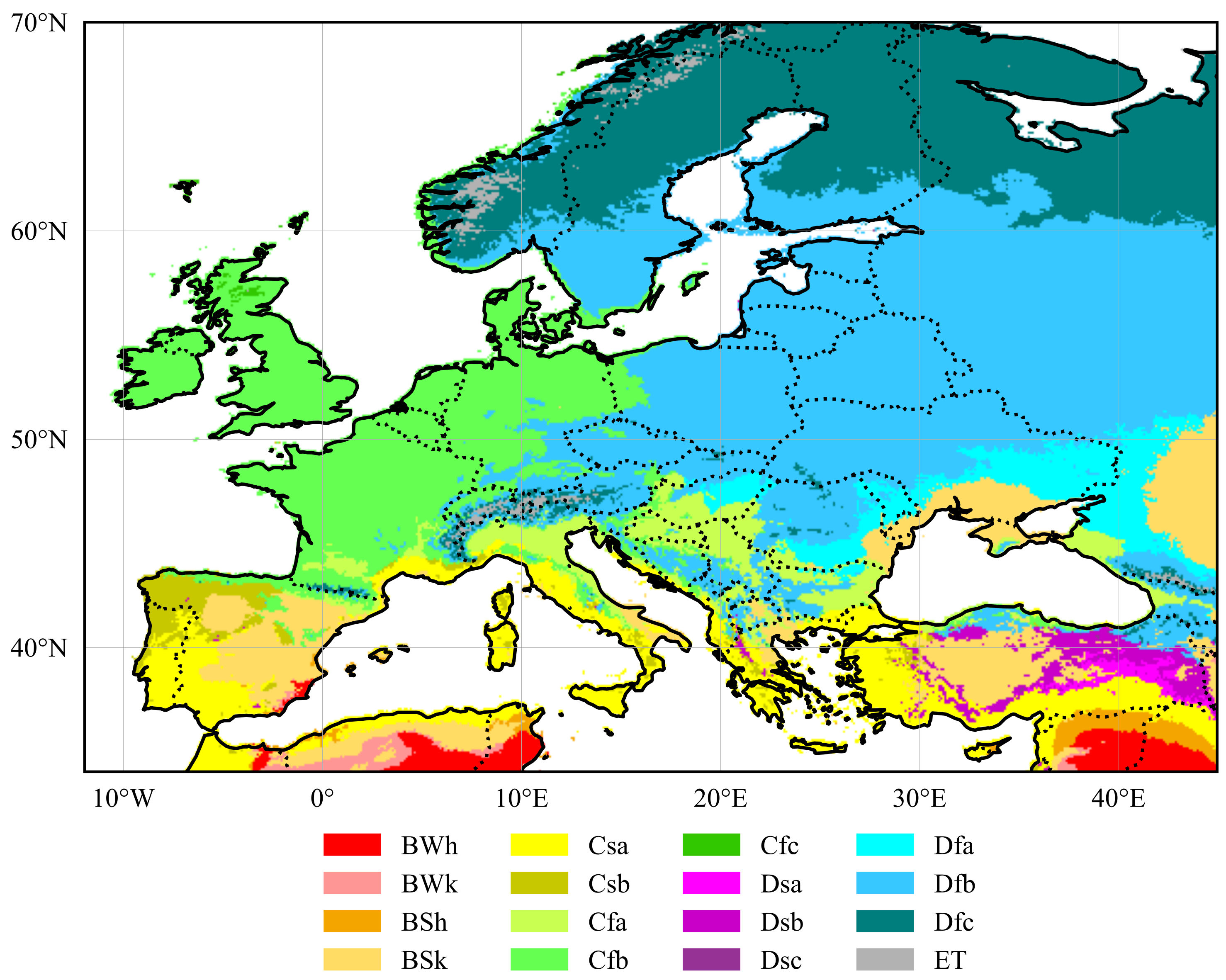
Figure 1. The proposed deployment pipeline of our system for isoprene emission SR, leveraging additional emission drivers in the SR process.
Remotesensing 17 01715 g001
Figure 2. The proposed training pipeline of our system for isoprene emission SR, leveraging additional emission drivers in the SR process.
Remotesensing 17 01715 g002
Figure 3. The study area adopted in this work; the map reports a monthly averaged isoprene emission (April 2019) from the TD-TROPO-010 inventory. Emission is reported as molec . cm 2 s .
Remotesensing 17 01715 g003
Figure 4. The CL (a), TC (b) percentage maps and LAI information (c) over the study area from the LC-ESA and LAI-TROPO-010 inventories, respectively. For the LAI map in (c), we report a monthly averaged value (April 2019).
Remotesensing 17 01715 g004
Figure 5. Geographical distribution of the Köppen–Geiger climate classes that are present over the study area. Please refer to Table 1 for more information regarding the different climate classes.
Remotesensing 17 01715 g005
Figure 6. The considered Köppen–Geiger climate classes for each S \ c c folds and their occurrences (number of patches) over the study area.
Remotesensing 17 01715 g006
Figure 7. Geographical distribution of patches for each fold S \ c c .
Remotesensing 17 01715 g007
Figure 8. Geographical distribution of patches for each fold S \ c c , associated with the standard (train and validation patches), unseen spatial areas, and unseen climate zones scenarios.
Remotesensing 17 01715 g008
Figure 9. Normalized temporal evolution of LAI and isoprene intensity (patch averaged), and PCC between isoprene and LAI intensity (patch averaged).
Remotesensing 17 01715 g009
Figure 10. Spatial correlation, measured using the PCC, of isoprene emissions with LAI ( ρ isop . , LAI ), CL ( ρ isop . , CL ), and TC ( ρ isop . , TC ) information. Vertical dashed lines denote the mean value μ of the related distribution.
Remotesensing 17 01715 g010
Figure 11. Conditional entropy of isoprene emissions with LAI ( H ( isop . | LAI ) ), CL ( H ( isop . | CL ) ) and TC ( H ( isop . | TC ) ) information. Vertical dashed lines denote the mean value μ of the related distribution.
Remotesensing 17 01715 g011
Figure 12. NIR from both the SR networks, considering the tree proposed input configurations and the four folds S \ c c . The improvement is computed using (5), considering the { Isop . } configuration (1-channel) in (1) as a reference method.
Remotesensing 17 01715 g012
Figure 13. Violin plot for the transformed (upper) and isoprene (bottom) emission data domain, for the HAT (a) and SAN (b) network, considering the four different input configurations and folds S \ c c .
Remotesensing 17 01715 g013
Figure 14. Super-resolved emission map examples ( I ^ HR ) from both the considered SR networks and all the four different input configurations. The first column shows the LR emission I LR ; the last column reports the ground-truth emission I HR . The other columns report I ^ HR for each configuration. Emissions are reported as molec . cm 2 s .
Remotesensing 17 01715 g014
Figure 15. Results comparing the standard, unseen spatial area, and unseen climate zone scenarios for both the SR networks. The reported NMSE is the average NMSE among all the folds S \ c c of S . The black segment denotes the standard deviation for each experiment.
Remotesensing 17 01715 g015
Figure 16. Super-resolved emission map examples ( I ^ HR ) from both the considered SR networks and all the four different input configurations. Patches are related to the unseen spatial area (a) and climate zone (b) scenarios. The first column shows the LR emission I LR ; the last column reports the ground-truth emission I HR . Emissions are reported as molec . cm 2 s .
Remotesensing 17 01715 g016
Table 1. Overview of the Köppen–Geiger climate classes that are present over the study area. Please refer to the original work in [76] for the defining criteria of each class.
Climate ClassDescription
BWhArid, desert, hot
BWkArid, desert, cold
BShArid, steppe, hot
BSkArid, steppe, cold
CsaTemperate, dry summer, hot summer
CsbTemperate, dry summer, warm summer
CfaTemperate, no dry season, hot summer
CfbTemperate, no dry season, warm summer
CfcTemperate, no dry season, cold summer
DsaCold, dry summer, hot summer
DsbCold, dry summer, warm summer
DscCold, dry summer, cold summer
DfaCold, no dry season, hot summer
DfbCold, no dry season, warm summer
DfcCold, no dry season, cold summer
ETPolar, tundra
Table 2. SR performance results evaluated on T ^ HR , i.e., transformed data domain. Avg and Std denote the average and standard deviation of the specific metric, respectively. In bold, we denote the best-performing average value, and underlined values denote the second-best, for each fold S \ c c for both the SR networks. Arrow direction (↑ or ↓) indicates the preferred direction for each metric.
Transformed Data Domain (Avg, Std)
ModelData FoldConfigurationNMSE ↓SSIM ↑PSNR ↑MaxAE ↓UIQI ↑SCC ↑
HAT S \ C f b { Isop . } −35.04, 6.420.98, 0.0538.11, 5.020.04, 0.040.97, 0.090.98, 0.06
{ Isop . , CL } −27.79, 5.710.94, 0.0830.86, 4.290.10, 0.060.94, 0.110.94, 0.09
{ Isop . , TC } −30.14, 6.020.96, 0.0733.21, 4.610.07, 0.050.96, 0.100.96, 0.07
{ Isop . , CL , TC } −36.69, 6.480.99, 0.0439.76, 5.050.04, 0.040.98, 0.090.99, 0.04
S \ D f b { Isop . } −36.23, 7.040.98, 0.0639.69, 5.550.03, 0.020.98, 0.100.98, 0.06
{ Isop . , CL } −35.43, 6.930.98, 0.0738.89, 5.370.04, 0.030.97, 0.110.98, 0.07
{ Isop . , TC } −35.21, 6.630.98, 0.0638.67, 5.110.04, 0.030.97, 0.100.98, 0.06
{ Isop . , CL , TC } −37.42, 7.220.99, 0.0540.89, 5.580.03, 0.020.98, 0.100.99, 0.05
S \ D f c { Isop . } −34.68, 5.800.99, 0.0437.88, 4.450.04, 0.040.98, 0.080.98, 0.05
{ Isop . , CL } −33.39, 5.790.98, 0.0436.6, 4.430.05, 0.040.98, 0.080.98, 0.05
{ Isop . , TC } −28.16, 5.420.95, 0.0731.36, 4.030.08, 0.060.95, 0.090.95, 0.07
{ Isop . , CL , TC } −36.12, 5.890.99, 0.0339.32, 4.550.04, 0.030.98, 0.080.99, 0.04
S \ M e d { Isop . } −33.81, 6.170.98, 0.0436.84, 4.820.05, 0.040.97, 0.080.98, 0.05
{ Isop . , CL } −29.85, 5.920.96, 0.0632.89, 4.550.07, 0.050.96, 0.090.96, 0.07
{ Isop . , TC } −36.28, 6.130.99, 0.0339.31, 4.800.04, 0.030.98, 0.080.99, 0.03
{ Isop . , CL , TC } −35.10, 6.220.99, 0.0438.14, 4.880.04, 0.040.98, 0.080.98, 0.04
SAN S \ C f b { Isop . } −24.93, 4.900.90, 0.1128.00, 3.670.13, 0.090.89, 0.130.88, 0.13
{ Isop . , CL } −25.80, 5.560.91, 0.1128.87, 4.300.12, 0.080.91, 0.120.90, 0.11
{ Isop . , TC } −24.52, 5.420.90, 0.1127.59, 4.120.14, 0.100.90, 0.130.89, 0.11
{ Isop . , CL , TC } −28.07, 6.170.94, 0.0931.14, 4.850.09, 0.060.94, 0.110.94, 0.09
S \ D f b { Isop . } −26.84, 5.000.94, 0.1030.30, 3.730.10, 0.080.94, 0.120.93, 0.12
{ Isop . , CL } −29.99, 5.890.96, 0.0933.45, 4.620.08, 0.070.96, 0.110.96, 0.09
{ Isop . , TC } −29.96, 5.880.96, 0.0933.42, 4.550.07, 0.070.96, 0.110.96, 0.08
{ Isop . , CL , TC } −32.13, 6.000.97, 0.0735.59, 4.600.06, 0.060.97, 0.10.97, 0.07
S \ D f c { Isop . } −23.62, 4.390.89, 0.1026.83, 3.180.17, 0.120.89, 0.130.87, 0.13
{ Isop . , CL } −23.71, 5.040.89, 0.1126.92, 3.820.18, 0.120.90, 0.120.89, 0.11
{ Isop . , TC } −25.37, 5.420.92, 0.1028.57, 4.140.13, 0.090.92, 0.110.91, 0.1
{ Isop . , CL , TC } −30.01, 6.670.96, 0.0833.21, 5.350.07, 0.060.95, 0.10.96, 0.07
S \ M e d { Isop . } −25.76, 5.230.91, 0.1028.79, 4.050.13, 0.090.91, 0.130.90, 0.13
{ Isop . , CL } −26.33, 5.710.92, 0.1029.37, 4.510.12, 0.090.92, 0.120.92, 0.11
{ Isop . , TC } −23.81, 5.090.89, 0.1126.84, 3.900.17, 0.110.90, 0.130.88, 0.11
{ Isop . , CL , TC } −27.44, 6.180.94, 0.1030.48, 4.930.10, 0.070.93, 0.110.93, 0.09
Table 3. SR performance results evaluated on I ^ HR , i.e., isoprene data domain. Avg and Std denote the average and standard deviation of the specific metric, respectively. In bold, we denote the best-performing average value, and underlined values denote the second-best, for each fold S \ c c for both the SR networks. Arrow direction (↑ or ↓) indicates the preferred direction for each metric.
Isoprene Data Domain (Avg, Std)
ModelData FoldConfigurationNMSE ↓SSIM ↑PSNR ↑MaxAE ↓UIQI ↑SCC ↑
HAT S \ C f b { Isop . } −17.35, 12.830.94, 0.1529.85, 11.93204.68, 555.710.70, 0.400.94, 0.11
{ Isop . , CL } −9.17, 13.510.85, 0.2121.67, 12.83281.33, 643.930.62, 0.400.86, 0.14
{ Isop . , TC } −11.83, 12.960.89, 0.1924.33, 12.22250.26, 610.560.66, 0.400.90, 0.12
{ Isop . , CL , TC } −19.42, 12.580.95, 0.1431.92, 11.76182.35, 526.540.71, 0.400.96, 0.10
S \ D f b { Isop . } −17.80, 15.170.92, 0.1830.03, 14.40345.73, 706.110.84, 0.290.94, 0.13
{ Isop . , CL } −17.07, 14.990.91, 0.1829.30, 14.19345.61, 706.910.83, 0.290.93, 0.14
{ Isop . , TC } −16.80, 14.850.91, 0.1829.03, 14.15346.54, 707.770.83, 0.300.93, 0.13
{ Isop . , CL , TC } −19.47, 14.630.93, 0.1531.70, 13.87318.25, 679.180.85, 0.280.94, 0.13
S \ D f c { Isop . } −16.93, 12.300.94, 0.1529.82, 11.58149.16, 386.150.70, 0.400.95, 0.10
{ Isop . , CL } −15.47, 12.250.93, 0.1728.36, 11.59154.12, 392.450.69, 0.400.94, 0.10
{ Isop . , TC } −9.04, 12.860.86, 0.2221.93, 12.36199.73, 442.250.63, 0.400.88, 0.13
{ Isop . , CL , TC } −18.76, 11.820.95, 0.1431.65, 11.16131.37, 363.450.71, 0.390.96, 0.09
S \ M e d { Isop . } −15.72, 14.090.93, 0.1727.54, 13.31217.76, 577.690.67, 0.410.93, 0.12
{ Isop . , CL } −10.95, 14.750.88, 0.2122.77, 14.09263.47, 629.470.63, 0.410.89, 0.14
{ Isop . , TC } −18.98, 13.350.95, 0.1430.79, 12.57182.40, 531.770.69, 0.400.96, 0.10
{ Isop . , CL , TC } −17.52, 13.710.94, 0.1629.33, 12.97196.47, 550.800.68, 0.410.95, 0.11
SAN S \ C f b { Isop . } −5.34, 14.030.77, 0.2417.84, 13.54337.51, 695.520.55, 0.390.76, 0.19
{ Isop . , CL } −6.47, 13.610.80, 0.2318.97, 13.31314.10, 675.290.59, 0.390.79, 0.18
{ Isop . , TC } −5.17, 13.770.77, 0.2417.67, 13.34326.66, 686.390.56, 0.390.76, 0.17
{ Isop . , CL , TC } −8.86, 13.960.84, 0.2421.37, 13.52281.56, 644.700.62, 0.400.85, 0.15
S \ D f b { Isop . } −7.54, 14.410.80, 0.2619.77, 13.95450.83, 793.870.72, 0.340.81, 0.18
{ Isop . , CL } −11.54, 14.070.86, 0.2223.77, 13.65380.77, 739.760.78, 0.310.88, 0.16
{ Isop . , TC } −11.90, 13.490.87, 0.2124.13, 12.94364.04, 726.350.79, 0.310.88, 0.15
{ Isop . , CL , TC } −14.21, 13.660.89, 0.1926.44, 13.09345.90, 708.960.81, 0.300.91, 0.14
S \ D f c { Isop . } −4.18, 13.460.76, 0.2517.07, 13.06248.90, 485.880.53, 0.390.75, 0.18
{ Isop . , CL } −4.05, 13.410.76, 0.2516.94, 13.16244.59, 481.940.56, 0.390.77, 0.17
{ Isop . , TC } −6.25, 12.950.80, 0.2419.14, 12.52220.32, 462.370.59, 0.400.81, 0.16
{ Isop . , CL , TC } −11.44, 13.150.88, 0.2224.32, 12.58179.76, 423.170.66, 0.400.90, 0.13
S \ M e d { Isop . } −5.40, 16.360.79, 0.2617.21, 15.94339.18, 699.780.55, 0.400.79, 0.19
{ Isop . , CL } −6.68, 15.720.81, 0.2618.50, 15.35306.36, 671.010.57, 0.410.82, 0.17
{ Isop . , TC } −3.21, 16.320.75, 0.2715.02, 16.09354.69, 711.830.53, 0.400.77, 0.17
{ Isop . , CL , TC } −8.18, 15.280.83, 0.2519.99, 14.86279.92, 646.750.60, 0.410.85, 0.16
Table 4. Training runtimes of all the experiments, therefore considering all the different configurations, folds, and SR networks.
Training Runtimes
HATSAN
Data FoldConfigurationEpochsTime [min]EpochsTime [min]
S \ C f b { Isop . } 499184772452
{ Isop . , CL } 7528069452
{ Isop . , TC } 8832266430
{ Isop . , CL , TC } 307114872490
S \ D f b { Isop . } 679256167440
{ Isop . , CL } 729282869466
{ Isop . , TC } 666263469467
{ Isop . , CL , TC } 614229078500
S \ D f c { Isop . } 499184369436
{ Isop . , CL } 499184664439
{ Isop . , TC } 7728067442
{ Isop . , CL , TC } 49918401491043
S \ M e d { Isop . } 499185972487
{ Isop . , CL } 8531169466
{ Isop . , TC } 483179865430
{ Isop . , CL , TC } 499185469438
Disclaimer/Publisher’s Note: The statements, opinions and data contained in all publications are solely those of the individual author(s) and contributor(s) and not of MDPI and/or the editor(s). MDPI and/or the editor(s) disclaim responsibility for any injury to people or property resulting from any ideas, methods, instructions or products referred to in the content.

