
A Review of High-Sensitivity Tracking Techniques for Satellite Navigation Signals
 , , , and
Abstract

1. Introduction
2. Methods
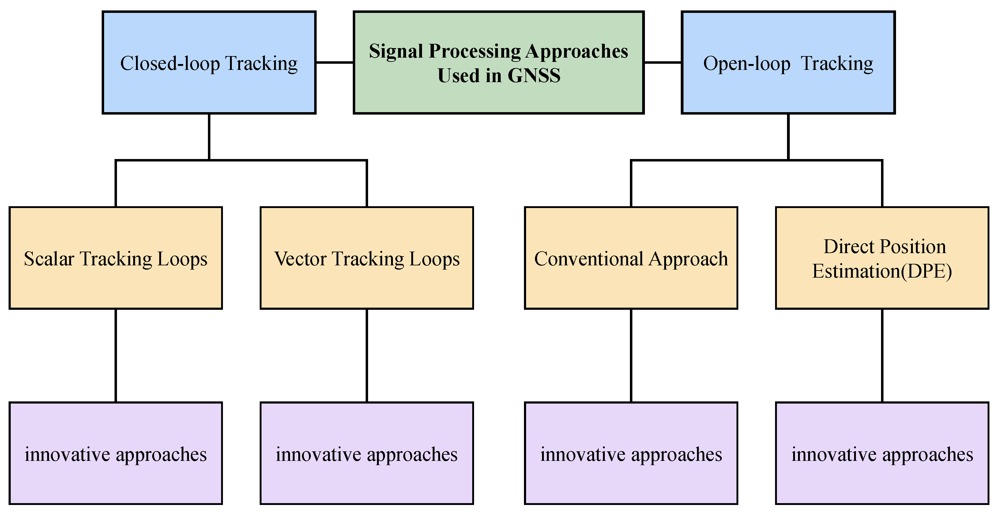
2.1. Tracking Methods
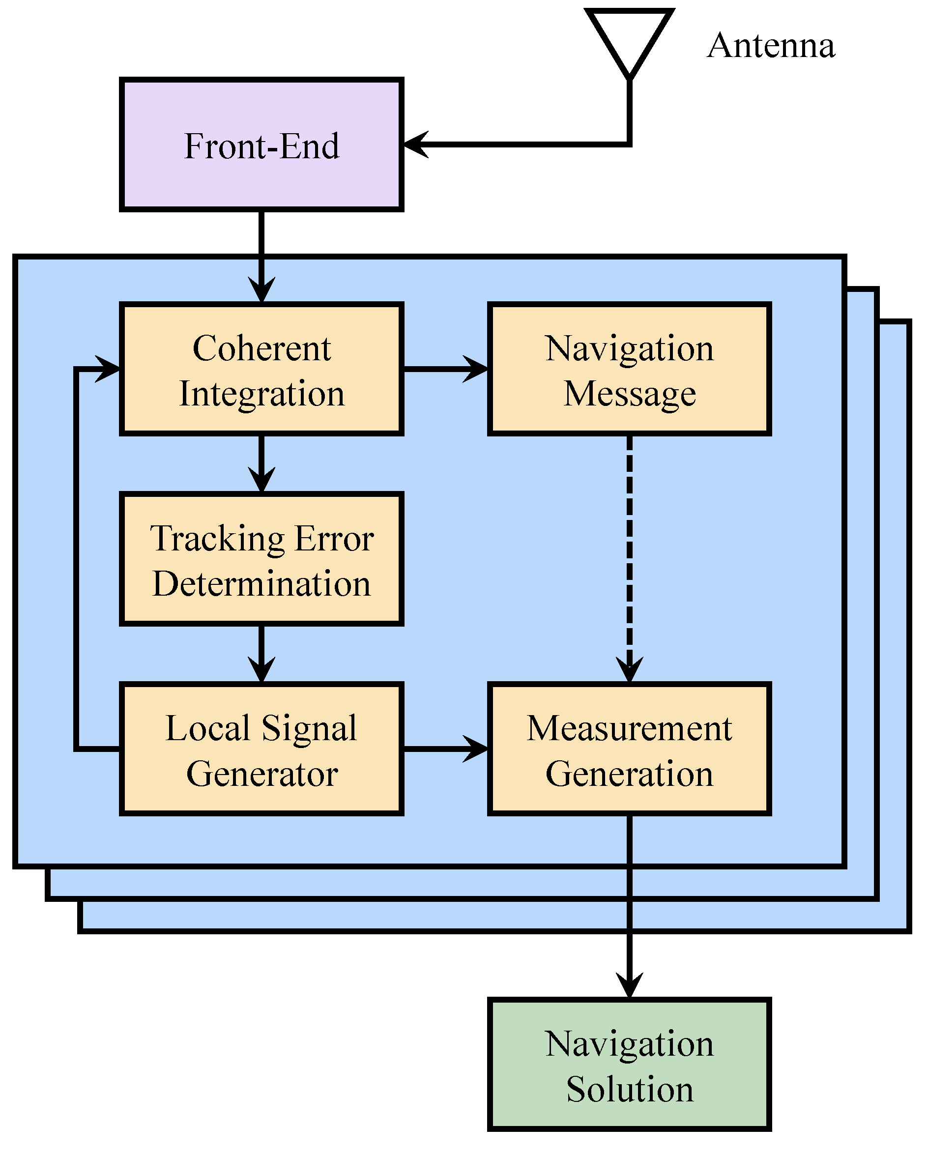
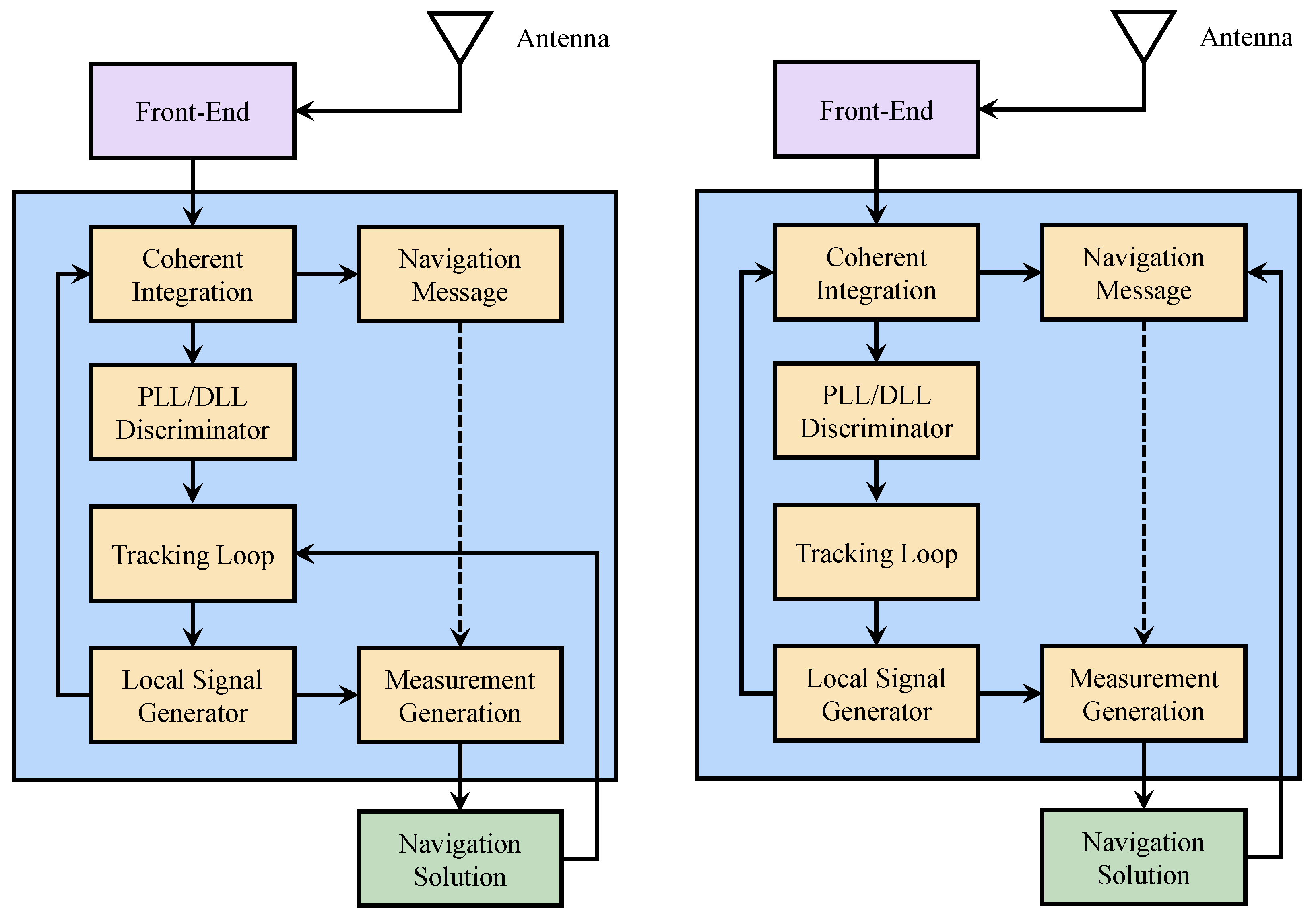
2.2. Scalar Tracking

| Tracking Method | Core Concept | Advantages | Limitations | Representative References |
|---|---|---|---|---|
| Scalar Tracking | Each satellite channel is tracked independently without exploiting inter-satellite geometry. | Simple structure; low computational cost. | Poor performance in dynamic or degraded environments; no channel cooperation. | Zhodzishsky, M. (1998) [19], Spilker Jr, J. (1996) [13], Pany, T. (2005) [20], Lian, P. (2005) [21], Ziedan, N. I. (2004) [10], Ren, T. (2012) [22], Curran, J. T. (2012) [23], Sun, Z. (2013) [24], Guo, W. (2014) [25], Yan, K. (2016) [11], Chen, S. (2017) [26], Li, J. (2018) [27], Feng, X. (2023) [12] |
| Vector Tracking | Navigation solution derived from all channels jointly feeds back into all loops, utilizing inter-channel geometric relationships. | Robust tracking in weak signal scenarios; better accuracy. | Complex navigation filter; sensitive to modeling errors. | Copps, D. B. (1980) [28], Lashley, M. (2007) [29], Lashley, M. (2009) [30], Lashley, M. (2009) [31], Lashley, M. (2010) [32], Henkel, P. (2009) [33], Chen, Q. (2014) [34], Peng, S. (2012) [35], Yang, H. (2021) [36], Farhad, M. (2021) [37], Mou, M. (2021) [14], Liu, W. (2022) [38], Marcal, J. (2016) [39], Lin, H. (2017) [40], Chen, Q. (2018) [41] |
| Open-Loop Tracking | Signal parameters are estimated through feedforward processing without feedback loops. | High observability; robust re-acquisition in fading. | High computational complexity; less suitable for real-time use. | Van Graas, F. (2005) [42], Anyaegbu, E. (2006) [43], Yan, K. (2016) [11], Tahir, M. (2012) [44], Jin, T. (2020) [45], Wu, C. (2022) [46], Stienne, G. (2012) [47], Closas, P. (2007) [48], Tahir, M. (2012) [49] |
| Direct Position Estimation | Jointly estimates position directly from raw signals without intermediate synchronization steps. | High positioning accuracy; bypasses code/carrier synchronization. | Computationally expensive; limited practical deployment. | Closas, P. (2007) [48], Closas, P. (2008) [50], Closas, P. (2009) [51], Closas, P. (2010) [52], Closas, P. (2017) [53], Amar, A. (2008) [54], Ramesh Kumar, A. (2015) [55], Ng, Y. (2016) [56], Chu, A. H.-P. (2019) [57] |
2.2.1. Extending Coherent Integration Time
2.2.2. Optimizing the Discriminator
2.2.3. Optimizing the Loop Filter
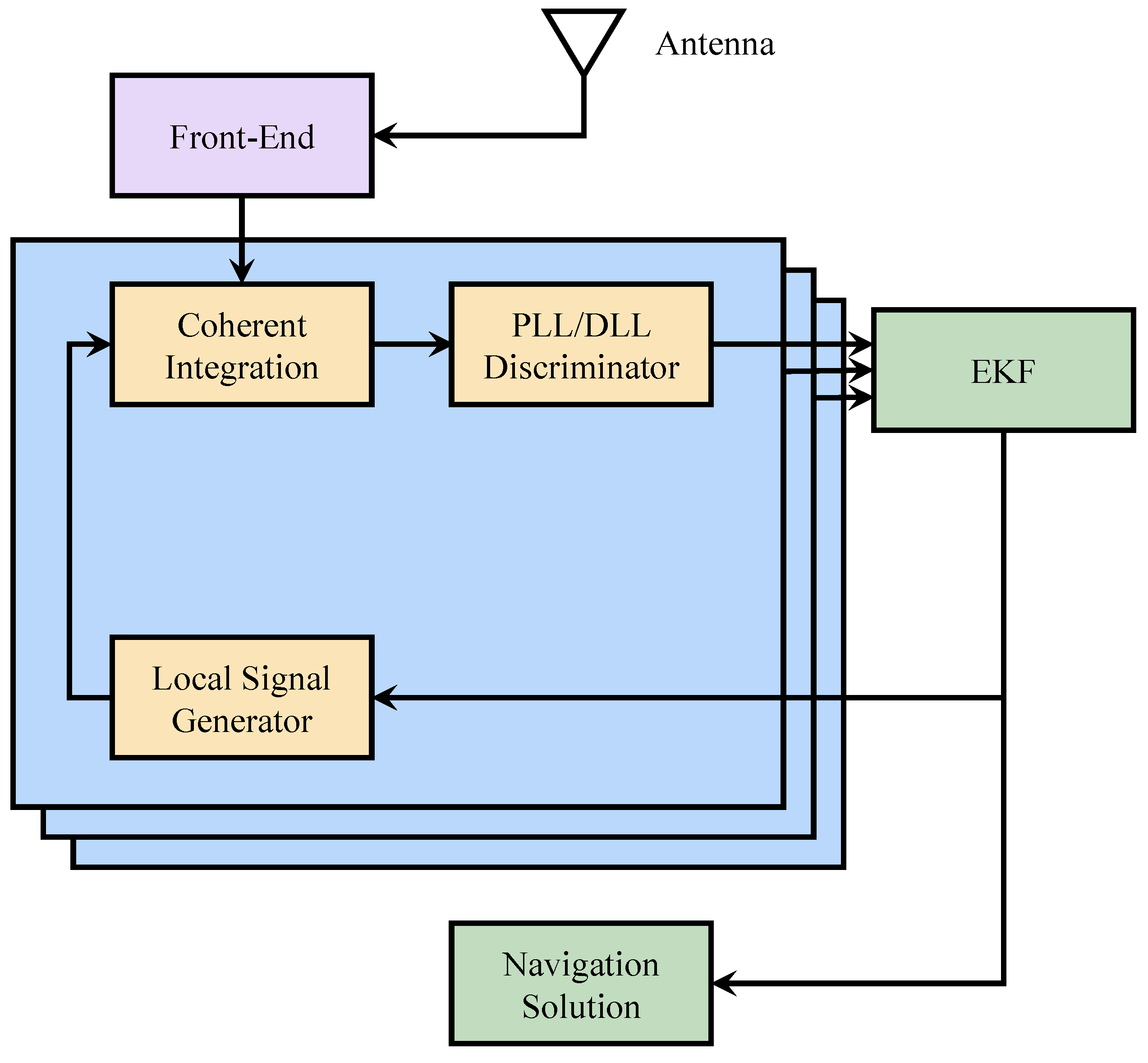
2.3. Vector Tracking Loops
2.3.1. Evolution of Vector Tracking Technique
2.3.2. Optimizing the Navigation Filter
2.3.3. Vector–Scalar Hybrid Tracking
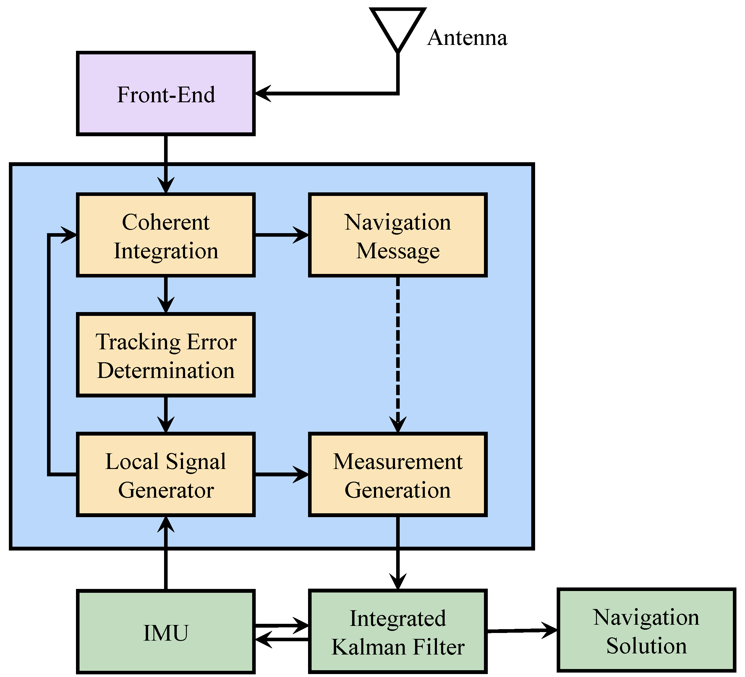
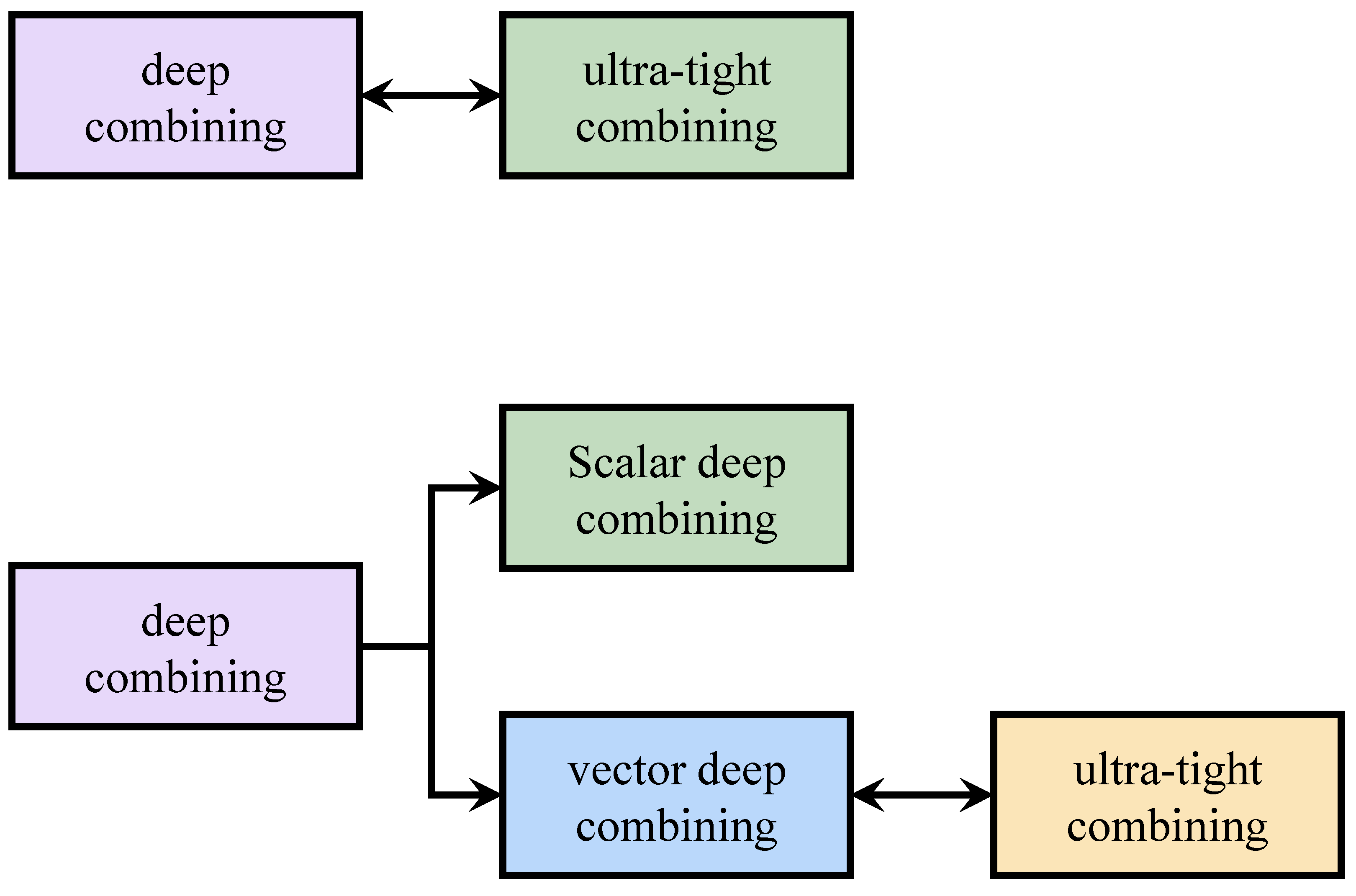
2.3.4. Ultra-Tight Combining
2.4. Conventional Approach
2.4.1. Improving Discriminator Estimation Precision
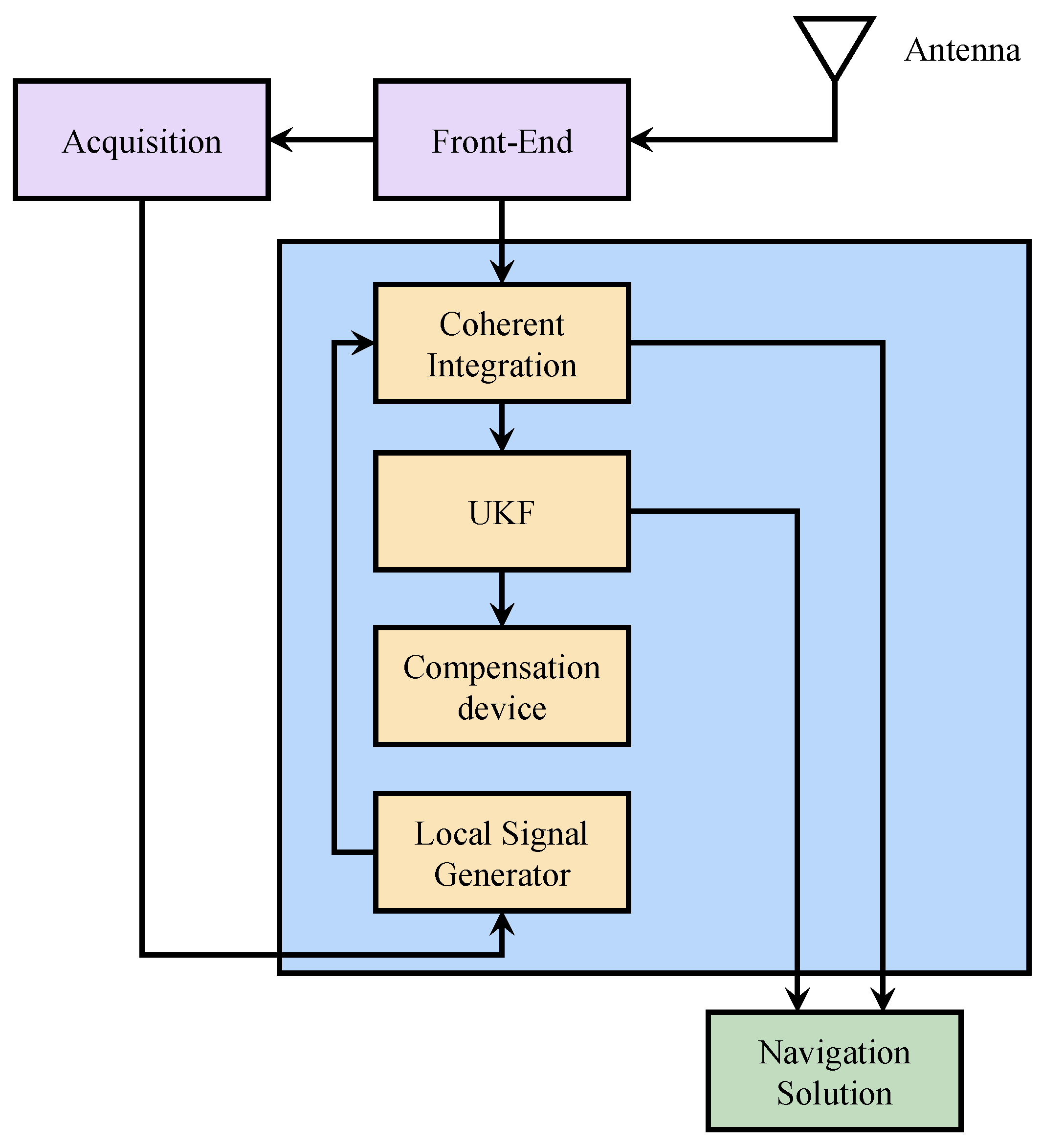
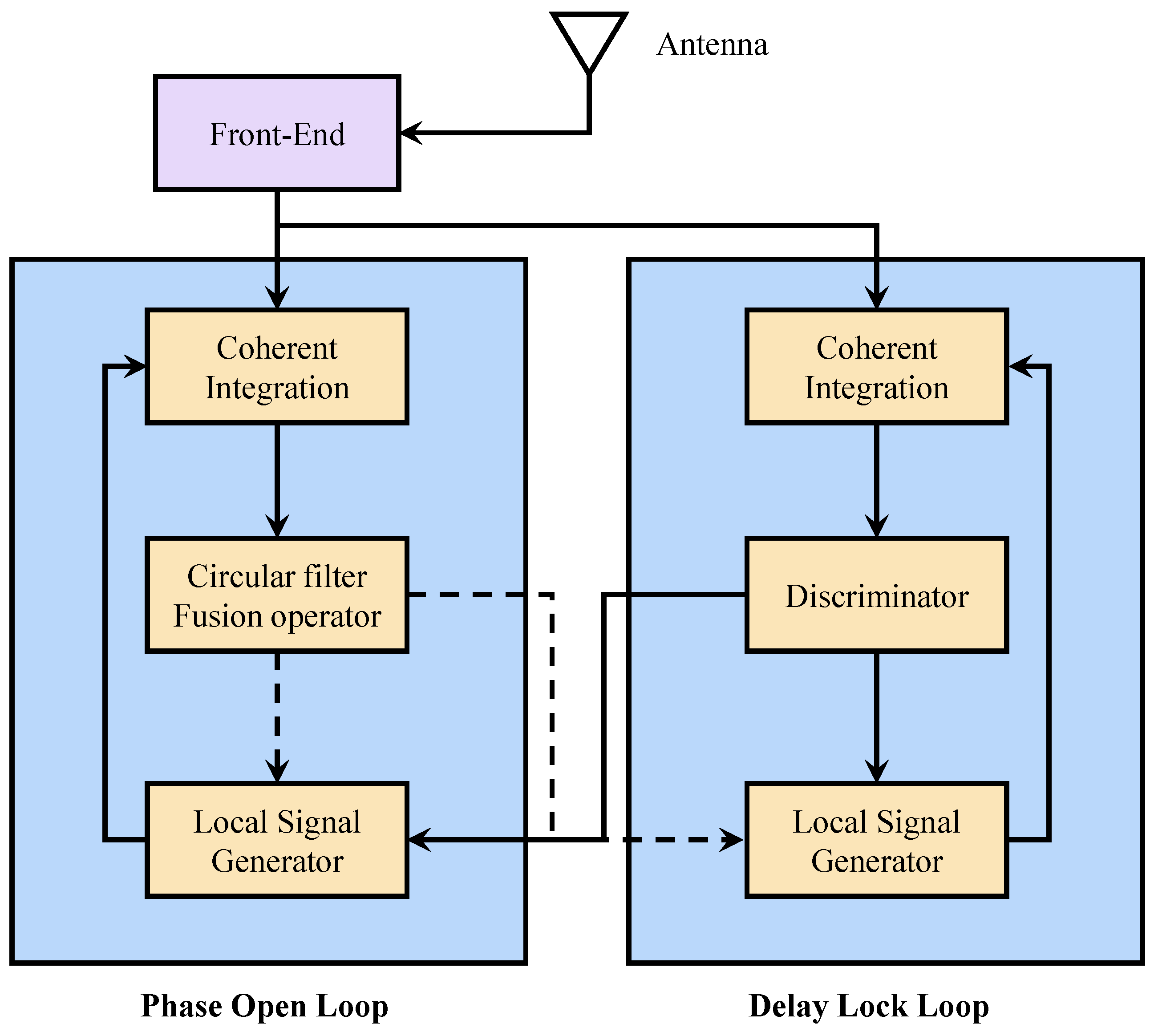
2.4.2. Open-Loop and Closed-Loop Hybrid Tracking
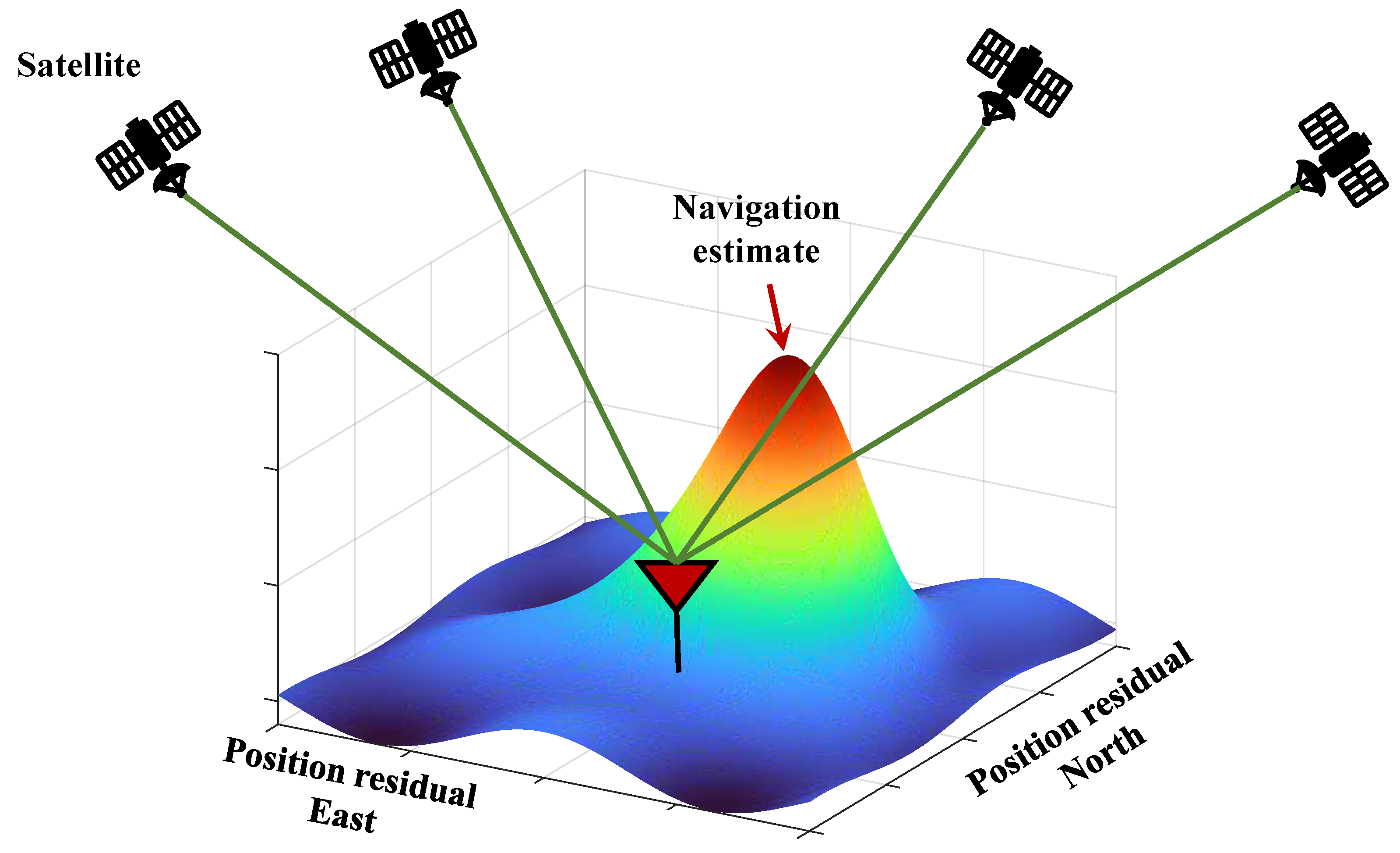
Direct Position Estimation
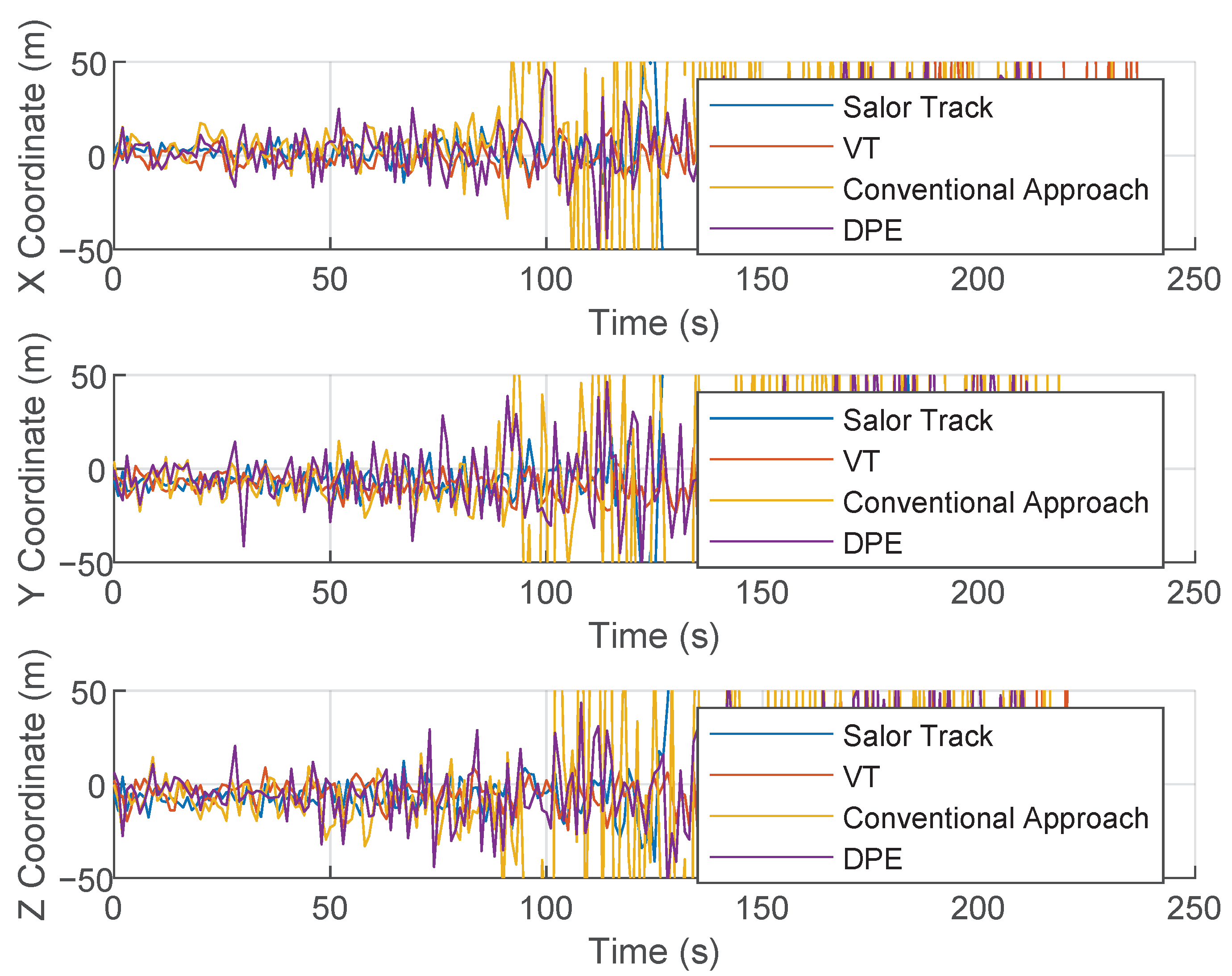
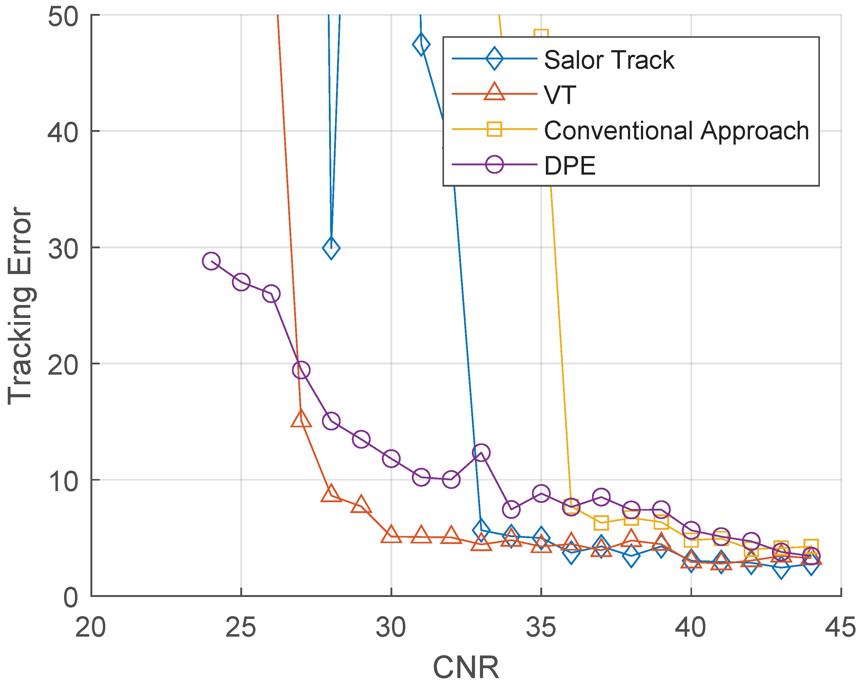
3. Results
4. Conclusions
- Integrating deep learning techniques into filter structures to enhance adaptability and robustness. Deep learning has the capability to model and adaptively adjust signal characteristics under various environmental conditions, thereby achieving more accurate state estimation in complex and dynamic channel environments. By incorporating deep learning algorithms, the parameters of the filters can be dynamically adjusted to maintain optimal performance in challenging scenarios;
- Current research on collaborative estimation schemes requires strong signals, but complex scenarios are often characterized by weak signals [12]. Therefore, there is a need to continue developing multi-channel collaborative estimation schemes for oscillator noise. By integrating external signal data, such as 4G/5G communication signals, the impact of oscillator noise on the signal can be reduced, coherent integration time can be extended, and the overall system performance can be improved;
- Design low-complexity approximations for open-loop tracking to better align with hardware resource constraints. By optimizing the algorithm structure and simplifying the computational process, it is possible to reduce the computational complexity of open-loop tracking without significantly compromising sensitivity and dynamic performance, thereby enhancing its feasibility for practical deployment;
Author Contributions
Funding
Data Availability Statement
Conflicts of Interest
References
- Hameed, A.; Ahmed, H.A. Survey on indoor positioning applications based on different technologies. In Proceedings of the 2018 12th International Conference on Mathematics, Actuarial Science, Computer Science and Statistics (MACS), Karachi, Pakistan, 24–25 November 2018; IEEE: Piscataway, NJ, USA, 2018; pp. 1–5. [Google Scholar]
- Gao, Z.; Shen, W.; Zhang, H.; Niu, X.; Ge, M. Real-time kinematic positioning of INS tightly aided multi-GNSS ionospheric constrained PPP. Sci. Rep. 2016, 6, 30488. [Google Scholar] [CrossRef] [PubMed]
- Canales, J. Navigating the history of GPS. Nat. Electron. 2018, 1, 610–611. [Google Scholar] [CrossRef]
- Rezwan, S.; Choi, W. Artificial intelligence approaches for UAV navigation: Recent advances and future challenges. IEEE Access 2022, 10, 26320–26339. [Google Scholar] [CrossRef]
- Kaplan, E.D.; Hegarty, C. Understanding GPS/GNSS: Principles and Applications; Artech House: Norwood, MA, USA, 2017. [Google Scholar]
- Ding, X.; Yang, Y.; Chen, J. Improved high-sensitivity partial-matched filter with FFT-based acquisition algorithm for BDS-2 and BDS-3 signals with secondary code modulation. GPS Solut. 2023, 27, 143. [Google Scholar] [CrossRef]
- Kuutti, S.; Fallah, S.; Katsaros, K.; Dianati, M.; Mccullough, F.; Mouzakitis, A. A survey of the state-of-the-art localization techniques and their potentials for autonomous vehicle applications. IEEE Internet Things J. 2018, 5, 829–846. [Google Scholar] [CrossRef]
- Ye, Z.; Zhao, G.; Yang, M.; Chen, P.-Y. Review on wearable antennas: Part 2: Recent advances and applications. IEEE Antennas Propag. Mag. 2025, 2–13. [Google Scholar] [CrossRef]
- Ashraf, I.; Hur, S.; Park, Y. Smartphone sensor based indoor positioning: Current status, opportunities, and future challenges. Electronics 2020, 9, 891. [Google Scholar] [CrossRef]
- Ziedan, N.I.; Garrison, J.L. Extended Kalman filter-based tracking of weak GPS signals under high dynamic conditions. In Proceedings of the 17th International Technical Meeting of the Satellite Division of the Institute of Navigation (ION GNSS 2004), Long Beach, CA, USA, 21–24 September 2004; pp. 20–31. [Google Scholar]
- Yan, K.; Ziedan, N.I.; Zhang, H.; Guo, W.; Niu, X.; Liu, J. Weak GPS signal tracking using FFT discriminator in open loop receiver. GPS Solut. 2016, 20, 225–237. [Google Scholar] [CrossRef]
- Feng, X.; Zhang, T.; Niu, X.; Pany, T.; Liu, J. Improving GNSS carrier phase tracking using a long coherent integration architecture. GPS Solut. 2023, 27, 37. [Google Scholar] [CrossRef]
- Spilker, J.J., Jr.; Axelrad, P.; Parkinson, B.W.; Enge, P. Global Positioning System: Theory and Applications, Volume I; American Institute of Aeronautics and Astronautics: Reston, VA, USA, 1996. [Google Scholar]
- Mou, M.; Hu, Y.; Gu, M.; Wang, S.; Liu, W. A vector tracking structure of FLL-assisted PLL for GNSS receiver. In Proceedings of the China Satellite Navigation Conference (CSNC 2021) Proceedings: Volume III, Nanchang, China, 22–25 May 2021; Springer: Berlin/Heidelberg, Germany, 2021; pp. 252–264. [Google Scholar]
- Van Graas, F.; Soloviev, A.; de Haag, M.U.; Gunawardena, S. Closed-loop sequential signal processing and open-loop batch processing approaches for GNSS receiver design. IEEE J. Sel. Top. Signal Process. 2009, 3, 571–586. [Google Scholar] [CrossRef]
- Meyr, H. Digital Communication Receivers: Synchronization, Channel Estimation, and Signal Processing; Wiley: Hoboken, NJ, USA, 1998. [Google Scholar]
- Kazemi, P.L. Optimum digital filters for GNSS tracking loops. In Proceedings of the 21st International Technical Meeting of the Satellite Division of The Institute of Navigation (ION GNSS 2008), Savannah, GA, USA, 16–19 September 2008; pp. 2304–2313. [Google Scholar]
- Van Diggelen, F. A-GPS: Assisted GPS, GNSS, and SBAS; Artech House: Norwood, MA, USA, 2009. [Google Scholar]
- Zhodzishsky, M.; Yudanov, S.; Veitsel, V.; Ashjaee, J. Co-op tracking for carrier phase. In Proceedings of the 11th International Technical Meeting of the Satellite Division of The Institute of Navigation (ION GPS 1998), Nashville, TN, USA, 15–18 September 1998; pp. 653–664. [Google Scholar]
- Pany, T.; Kaniuth, R.; Eissfeller, B. Deep integration of navigation solution and signal processing. In Proceedings of the 18th International Technical Meeting of the Satellite Division of The Institute of Navigation (ION GNSS 2005), Fort Worth, TX, USA, 25–28 September 2005; pp. 1095–1102. [Google Scholar]
- Lian, P.; Lachapelle, G.; Ma, C. Improving tracking performance of PLL in high dynamics applications. In Proceedings of the 2005 National Technical Meeting of the Institute of Navigation, San Diego, CA, USA, 22–24 January 2005; pp. 1042–1052. [Google Scholar]
- Ren, T.; Petovello, M.; Basnayake, C. Requirements analysis for bit synchronization and decoding in a standalone high-sensitivity GNSS receiver. In Proceedings of the 2012 Ubiquitous Positioning, Indoor Navigation, and Location Based Service (UPINLBS), Helsinki, Finland, 3–4 October 2012; IEEE: Piscataway, NJ, USA, 2012; pp. 1–9. [Google Scholar]
- Curran, J.T.; Lachapelle, G.; Murphy, C.C. Digital GNSS PLL design conditioned on thermal and oscillator phase noise. IEEE Trans. Aerosp. Electron. Syst. 2012, 48, 180–196. [Google Scholar] [CrossRef]
- Sun, X.; Qin, H.; Niu, J. Comparison and analysis of GNSS signal tracking performance based on Kalman filter and traditional loop. WSEAS Trans. Signal Process. 2013, 9, 99–107. [Google Scholar]
- Guo, W.; Yan, K.; Zhang, H.; Niu, X.; Shi, C. Double stage NCO-based carrier tracking loop in GNSS receivers for city environmental applications. IEEE Commun. Lett. 2014, 18, 1747–1750. [Google Scholar] [CrossRef]
- Chen, S.; Gao, Y.; Lin, T. Effect and mitigation of oscillator vibration-induced phase noise on carrier phase tracking. GPS Solut. 2017, 21, 1515–1524. [Google Scholar] [CrossRef]
- Li, J.; Zhao, L.; Hou, Y.; Hu, Y. A new tracking technique with the memory discriminator for high sensitivity GNSS receivers. In Proceedings of the 2018 IEEE 4th International Conference on Computer and Communications (ICCC), Chengdu, China, 7–10 December 2018; IEEE: Piscataway, NJ, USA, 2018; pp. 959–962. [Google Scholar]
- Copps, E.; Geier, G.; Fidler, W.; Grundy, P. Optimal processing of GPS signals. Navigation 1980, 27, 171–182. [Google Scholar] [CrossRef]
- Lashley, M.; Bevly, D.M. Analysis of discriminator based vector tracking algorithms. In Proceedings of the 2007 National Technical Meeting of the Institute of Navigation, San Diego, CA, USA, 22–24 January 2007; pp. 570–576. [Google Scholar]
- Lashley, M.; Bevly, D.M. Vector delay/frequency lock loop implementation and analysis. In Proceedings of the 2009 International Technical Meeting of The Institute of Navigation, Anaheim, CA, USA, 22–25 January 2009; pp. 1073–1086. [Google Scholar]
- Lashley, M.; Bevly, D.M.; Hung, J.Y. Performance analysis of vector tracking algorithms for weak GPS signals in high dynamics. IEEE J. Sel. Top. Signal Process. 2009, 3, 661–673. [Google Scholar] [CrossRef]
- Lashley, M.; Bevly, D.M.; Hung, J.Y. Analysis of deeply integrated and tightly coupled architectures. In Proceedings of the IEEE/ION Position, Location and Navigation Symposium, Portland, OR, USA, 20–23 April 2020; IEEE: Piscataway, NJ, USA, 2010; pp. 382–396. [Google Scholar]
- Henkel, P.; Giger, K.; Gunther, C. Multifrequency, multisatellite vector phase-locked loop for robust carrier tracking. IEEE J. Sel. Top. Signal Process. 2009, 3, 674–681. [Google Scholar] [CrossRef]
- Chen, X.; Wang, X.; Xu, Y. Performance enhancement for a GPS vector-tracking loop utilizing an adaptive iterated extended Kalman filter. Sensors 2014, 14, 23630–23649. [Google Scholar] [CrossRef]
- Peng, S.; Morton, Y.; Di, R. A multiple-frequency GPS software receiver design based on a vector tracking loop. In Proceedings of the 2012 IEEE/ION Position, Location and Navigation Symposium, Myrtle Beach, SC, USA, 23–26 April 2012; IEEE: Piscataway, NJ, USA, 2012; pp. 495–505. [Google Scholar]
- Yang, H.; Zhou, B.; Wang, L.; Wei, Q.; Ji, F.; Zhang, R. Performance and evaluation of GNSS receiver vector tracking loop based on adaptive cascade filter. Remote Sens. 2021, 13, 1477. [Google Scholar] [CrossRef]
- Farhad, M.; Mosavi, M.; Abedi, A. Fully adaptive smart vector tracking of weak GPS signals. Arab. J. Sci. Eng. 2021, 46, 1383–1393. [Google Scholar] [CrossRef]
- Liu, W.; Huang, H.; Hu, Y.; Mou, M.; Hsieh, T.H.; Hu, Q.; Wang, S. Improved GNSS vector tracking loop to enhance the navigation performance of USV. Ocean Eng. 2022, 258, 111865. [Google Scholar] [CrossRef]
- Marcal, J.; Nunes, F.; Sousa, F.M. Performance of a scintillation robust vector tracking for GNSS carrier phase signals. In Proceedings of the 2016 8th ESA Workshop on Satellite Navigation Technologies and European Workshop on GNSS Signals and Signal Processing (NAVITEC), Noordwijk, The Netherlands, 14–16 December 2016; IEEE: Piscataway, NJ, USA, 2016; pp. 1–8. [Google Scholar]
- Lin, H.; Huang, Y.; Tang, X.; Sun, G.; Ou, G. A robust vector tracking loop based on diagonal weighting matrix for navigation signal. Adv. Space Res. 2017, 60, 2607–2619. [Google Scholar] [CrossRef]
- Chen, Q.; Wu, X.; Liang, J.; Zeng, C. An EKF-based tracking loop filter algorithm in GNSS receiver for ultra high dynamic environment: The experiment results. In Proceedings of the IECON 2018-44th Annual Conference of the IEEE Industrial Electronics Society, Washington, DC, USA, 21-23 October 2018; pp. 2802–2808. [Google Scholar]
- Van Graas, F.; Soloviev, A.; de Haag, M.U.; Gunawardena, S.; Braasch, M. Comparison of two approaches for GNSS receiver algorithms: Batch processing and sequential processing considerations. In Proceedings of the 18th International Technical Meeting of the Satellite Division of The Institute of Navigation (ION GNSS 2005), Fort Worth, TX, USA, 25–28 September 2005; pp. 200–211. [Google Scholar]
- Anyaegbu, E. A frequency domain quasi-open loop tracking loop for GNSS receivers. In Proceedings of the 19th International Technical Meeting of the Satellite Division of The Institute of Navigation (ION GNSS 2006), Fort Worth, TX, USA, 26–29 September 2006; pp. 790–798. [Google Scholar]
- Tahir, M.; Presti, L.L.; Fantino, M. Characterizing different open loop fine frequency estimation methods for GNSS receivers. In Proceedings of the 2012 International Technical Meeting of The Institute of Navigation, Newport Beach, CA, USA, 30 January–1 February 2012; pp. 311–355. [Google Scholar]
- Jin, T.; Yuan, H.; Ling, K.-V.; Qin, H.; Kang, J. Differential Kalman filter design for GNSS open loop tracking. Remote Sens. 2020, 12, 812. [Google Scholar] [CrossRef]
- Wu, C.; Li, Y.; Luo, L.; Xie, J.; Wang, L. Two-step frequency estimation of GNSS signal in high-dynamic environment. Int. J. Antennas Propag. 2022, 2022, 1017206. [Google Scholar] [CrossRef]
- Stienne, G.; Reboul, S.; Choquel, J.-B.; Benjelloun, M. Circular data processing tools applied to a phase open loop architecture for multi-channels signals tracking. In Proceedings of the 2012 IEEE/ION Position, Location and Navigation Symposium, Myrtle Beach, SC, USA, 23–26 April 2012; IEEE: Piscataway, NJ, USA, 2012; pp. 633–642. [Google Scholar]
- Closas, P.; Fernández-Prades, C.; Fernández-Rubio, J.A. Maximum likelihood estimation of position in GNSS. IEEE Signal Process. Lett. 2007, 14, 359–362. [Google Scholar] [CrossRef]
- Tahir, M.; Presti, L.L.; Fantino, M. A novel quasi-open loop architecture for GNSS carrier recovery systems. Int. J. Navig. Obs. 2012, 2012, 324858. [Google Scholar] [CrossRef]
- Closas, P.; Fernandez-Prades, C.; Bernal, D.; Fernandez-Rubio, J.A. Bayesian direct position estimation. In Proceedings of the 21st International Technical Meeting of the Satellite Division of The Institute of Navigation (ION GNSS 2008), Savannah, GA, USA, 16–19 September 2008; pp. 183–190. [Google Scholar]
- Closas, P.; Fernandez-Prades, C.; Fernandez-Rubio, J.A. Cramér–Rao bound analysis of positioning approaches in GNSS receivers. IEEE Trans. Signal Process. 2009, 57, 3775–3786. [Google Scholar] [CrossRef]
- Closas, P.; Fernández-Prades, C. Bayesian nonlinear filters for direct position estimation. In Proceedings of the 2010 IEEE Aerospace Conference, Big Sky, MT, USA, 6–13 March 2010; IEEE: Piscataway, NJ, USA, 2010; pp. 1–12. [Google Scholar]
- Closas, P.; Gusi-Amigo, A. Direct position estimation of GNSS receivers: Analyzing main results, architectures, enhancements, and challenges. IEEE Signal Process. Mag. 2017, 34, 72–84. [Google Scholar] [CrossRef]
- Amar, A.; Weiss, A.J. New asymptotic results on two fundamental approaches to mobile terminal location. In Proceedings of the 2008 3rd International Symposium on Communications, Control and Signal Processing, St Julian’s, Malta, 12–14 March 2008; IEEE: Piscataway, NJ, USA, 2008; pp. 1320–1323. [Google Scholar]
- Ramesh Kumar, A. Direct Position Tracking in GPS Using Vector Correlator. Ph.D. Thesis, University of Illinois at Urbana-Champaign, Champaign, IL, USA, 2015. [Google Scholar]
- Ng, Y. Improving the Robustness of GPS Direct Position Estimation. Ph.D. Thesis, University of Illinois at Urbana-Champaign, Champaign, IL, USA, 2016. [Google Scholar]
- Chu, A.H.-P.; Chauhan, S.V.S.; Gao, G.X. GPS multireceiver direct position estimation for aerial applications. IEEE Trans. Aerosp. Electron. Syst. 2019, 56, 249–262. [Google Scholar] [CrossRef]
- Alban, S.; Akos, D.M.; Rock, S.M. Performance analysis and architectures for INS-aided GPS tracking loops. In Proceedings of the 2003 National Technical Meeting of The Institute of Navigation, Anaheim, CA, USA, 22–24 January 2003; pp. 611–622. [Google Scholar]
- Borio, D.; Sokolova, N.; Lachapelle, G. Memory discriminators for non-coherent integration in GNSS tracking loops. Proc. European Navigation Conf. ENC 2009, 9. Available online: https://api.semanticscholar.org/CorpusID:58704482 (accessed on 7 May 2025).
- Borio, D.; Lachapelle, G. A non-coherent architecture for GNSS digital tracking loops. Ann. Telecommun. Ann. Des TéLéCommunications 2009, 64, 601–614. [Google Scholar] [CrossRef]
- Xu, J. Beidou Satellite Navigation System Space Signal Interface Control Document Interpretation. Int. Space 2013, 26–32. Available online: http://www.beidou.gov.cn/yw/xwzx/201712/W020171226734109234149.pdf (accessed on 7 May 2025).
- Dunn, M.J.; Disl, D. Global Positioning System Directorate Systems Engineering & Integration Interface Specification IS-GPS-200; Global Positioning Systems Directorate: Los Angeles, CA, USA, 2012. [Google Scholar]
- Chen, J. Research on Performance Enhancement Technology of Inertial Beidou Deep Integrated Navigation Under High Dynamic Conditions. Ph.D. Thesis, Nanjing University of Aeronautics and Astronautics, Nanjing, China, 2019. [Google Scholar]
- Pany, T.; Riedl, B.; Winkel, J.; Wrz, T.; Jiménez-Baos, D. Coherent integration time: The longer, the better. Inside GNSS 2009, 4, 52–61. [Google Scholar]
- Bernal, D.; Closas, P.; Fernandez-Rubio, J.A. Particle filtering algorithm for ultra-tight GNSS/INS integration. In Proceedings of the 21st International Technical Meeting of the Satellite Division of The Institute of Navigation (ION GNSS 2008), Savannah, Georgia, 16–19 September 2008; pp. 2137–2144. [Google Scholar]
- Zhang, T.; Ban, Y.; Niu, X.; Guo, W.; Liu, J. Improving the design of MEMS INS-aided PLLs for GNSS carrier phase measurement under high dynamics. Micromachines 2017, 8, 135. [Google Scholar] [CrossRef]
- Niu, X.; Ban, Y.; Zhang, Q.; Zhang, T.; Zhang, H.; Liu, J. Quantitative analysis to the impacts of IMU quality in GPS/INS deep integration. Micromachines 2015, 6, 1082–1099. [Google Scholar] [CrossRef]
- Ren, T.; Petovello, M.G. A stand-alone approach for high-sensitivity GNSS receivers in signal-challenged environment. IEEE Trans. Aerosp. Electron. Syst. 2017, 53, 2438–2448. [Google Scholar] [CrossRef]
- Lindsey, W.C.; Chie, C.M. Theory of oscillator instability based upon structure functions. Proc. IEEE 1976, 64, 1652–1666. [Google Scholar] [CrossRef]
- Gaggero, P. Effect of Oscillator Instability on GNSS Signal Integration Time; University of Neuchtel: Neuchâtel, Switzerland, 2008. [Google Scholar]
- Gowdayyanadoddi, N.S.; Broumandan, A.; Curran, J.T.; Lachapelle, G. Benefits of an ultra stable oscillator for long coherent integration. In Proceedings of the 27th International Technical Meeting of The Satellite Division of the Institute of Navigation (ION GNSS+ 2014), Denver, CO, USA, 11–15 September 2014; pp. 1578–1594. [Google Scholar]
- Watson, R.; Lachapelle, G.; Klukas, R. Testing oscillator stability as a limiting factor in extreme high-sensitivity GPS applications. In Proceedings of the European Navigation Conference, Estoril, Portugal, 14–18 May 2006; Citeseer: Beijing, China, 2006; pp. 1–20. [Google Scholar]
- Irsigler, M.; Eissfeller, B. PLL tracking performance in the presence of oscillator phase noise. GPS Solut. 2002, 5, 45–57. [Google Scholar] [CrossRef]
- Pany, T.; Euler, H.-J.; Winkel, J. Indoor carrier phase tracking and positioning with difference correlators. In Proceedings of the 24th International Technical Meeting of the Satellite Division of The Institute of Navigation (ION GNSS 2011), Portland, OR, USA, 19–23 September 2011; pp. 2202–2213. [Google Scholar]
- Pany, T.; Euler, H.; Winkel, J. Difference correlators. In Does Indoor Carrier Phase Tracking Allow Indoor RTK. 2012, pp. 62–73. Available online: https://www.academia.edu/3064-9765/1/1/10.20935/AcadMolBioGen7288 (accessed on 7 May 2025).
- Li, Z. Research on Deep Integration Technology for GNSS Carrier Phase Quality in Complex Signal Environment; Wuhan University: Wuhan, China, 2019. [Google Scholar]
- Zhodzishsky, M.; Kurynin, R.; Veitsel, A. A radical approach to reducing effects of quartz crystal oscillator instability on GNSS receiver performance. In Proceedings of the 2020 Systems of Signal Synchronization, Generating and Processing in Telecommunications (SYNCHROINFO), Svetlogorsk, Russia, 1–3 July 2020; IEEE: Piscataway, NJ, USA, 2020; pp. 1–18. [Google Scholar]
- Borio, D.; Camoriano, L.; Presti, L.L.; Fantino, M. DTFT-based frequency lock loop for GNSS applications. IEEE Trans. Aerosp. Electron. Syst. 2008, 44, 595–612. [Google Scholar] [CrossRef]
- Palmer, L. Coarse frequency estimation using the discrete Fourier transform (corresp.). IEEE Trans. Inf. Theory 1974, 20, 104–109. [Google Scholar] [CrossRef]
- Yang, C. Tracking of GPS code phase and carrier frequency in the frequency domain. In Proceedings of the 16th International Technical Meeting of the Satellite Division of The Institute of Navigation (ION GPS/GNSS 2003), Fort Worth, TX, USA, 25–28 September 2003; pp. 628–637. [Google Scholar]
- Schamus, J.J.; Tsui, J.B.; Lin, D.M. Real-time software GPS receiver. In Proceedings of the 15th International Technical Meeting of the Satellite Division of The Institute of Navigation (ION GPS 2002), Portland, Oregon, 24–27 September 2002; pp. 2561–2565. [Google Scholar]
- Ba, X.; Liu, H.; Zheng, R.; Chen, J. A novel algorithm based on FFT for ultra high-sensitivity GPS tracking. In Proceedings of the 22nd International Technical Meeting of The Satellite Division of the Institute of Navigation (ION GNSS 2009), Savannah, GA, USA, 22–25 September 2009; pp. 1700–1706. [Google Scholar]
- Yan, K.; Zhang, T.; Niu, X.; Zhang, H.; Zhang, P.; Liu, J. INS-aided tracking with FFT frequency discriminator for weak GPS signal under dynamic environments. GPS Solut. 2017, 21, 917–926. [Google Scholar] [CrossRef]
- Wang, X.; Ji, X.; Feng, S.; Calmettes, V. A high-sensitivity GPS receiver carrier-tracking loop design for high-dynamic applications. GPS Solut. 2015, 19, 225–236. [Google Scholar] [CrossRef]
- Jiang, R.; Wang, K.; Liu, S.; Li, Y. Performance analysis of a Kalman filter carrier phase tracking loop. GPS Solut. 2017, 21, 551–559. [Google Scholar] [CrossRef]
- Liu, W.; Wu, L.; Hu, Y.; Huang, H.; Wang, S. GNSS/INS integrated navigation algorithm framework based on cascade vector tracking algorithm for USV. Mar. Geod. 2025, 48, 72–96. [Google Scholar] [CrossRef]
- Kim, K.-H.; Jee, G.-I.; Song, J.-H. Carrier tracking loop using the adaptive two-stage Kalman filter for high dynamic situations. Int. J. Control Autom. Syst. 2008, 6, 948–953. [Google Scholar]
- Yao, G.; Wu, W.; He, X. High dynamic carrier phase tracking based on adaptive Kalman filtering. In Proceedings of the 2011 Chinese Control and Decision Conference (CCDC), Mianyang, China, 23–25 May 2011; pp. 1245–1249. [Google Scholar]
- Cheng, Y.; Chang, Q. A carrier tracking loop using adaptive strong tracking Kalman filter in GNSS receivers. IEEE Commun. Lett. 2020, 24, 2903–2907. [Google Scholar] [CrossRef]
- Wang, Y.; Yang, R.; Morton, Y.J. Kalman filter-based robust closed-loop carrier tracking of airborne GNSS radio-occultation signals. IEEE Trans. Aerosp. Electron. Syst. 2020, 56, 3384–3393. [Google Scholar] [CrossRef]
- Tang, X.; Falco, G.; Falletti, E.; Presti, L.L. Practical implementation and performance assessment of an extended Kalman filter-based signal tracking loop. In Proceedings of the 2013 International Conference on Localization and GNSS (ICL-GNSS), Turin, Italy, 5–27 June 2013; IEEE: Piscataway, NJ, USA, 2013; pp. 1–6. [Google Scholar]
- Qin, H.; Liu, Y.; Jin, T. A novel adaptive EKF GNSS weak signal tracking algorithm. In Proceedings of the Conference on Navigation and Communication, Herndon, VA, USA, 11–13 May 2010. [Google Scholar]
- Zeng, C.; Li, W. Application of extended Kalman filter for tracking high dynamic GPS signal. In Proceedings of the IEEE International Conference on Signal Processing, Zhuhai, China, 22–24 November 2016. [Google Scholar]
- Psiaki, M.L.; Jung, H. Extended Kalman filter methods for tracking weak GPS signals. In Proceedings of the 15th International Technical Meeting of the Satellite Division of the Institute of Navigation (ION GPS 2002), Portland, OR, USA, 24–27 September 2002. [Google Scholar]
- Jung, H.; Psiaki, M.L.; Powell, S.P. Kalman-filter-based semi-codeless tracking of weak dual-frequency GPS signals. In Proceedings of the 16th International Technical Meeting of the Satellite Division of The Institute of Navigation (ION GPS/GNSS 2003), Portland, OR, USA, 12 September 2003. [Google Scholar]
- Zhu, Z.; Zhu, C.; Tang, G.; Li, S.; Huang, F. EKF based vector delay lock loop algorithm for GPS signal tracking. In Proceedings of the 2010 International Conference on Computer Design and Applications, Qinhuangdao, China, 25–27 June 2010. [Google Scholar]
- Lashley, M.; Bevly, D.M.; Hung, J.Y. A valid comparison of vector and scalar tracking loops. In Proceedings of the IEEE/ION Position, Location and Navigation Symposium, Indian Wells, CA, USA, 4–6 May 2010; pp. 464–474. [Google Scholar]
- Challa, S. Fundamentals of Object Tracking; Cambridge University Press: Cambridge, UK, 2011. [Google Scholar]
- Bhattacharyya, S. Performance and Integrity Analysis of the Vector Tracking Architecture of GNSS Receivers; University of Minnesota: Minneapolis, MN, USA, 2012. [Google Scholar]
- Lin, T.; O’Driscoll, C.; Lachapelle, G. Channel context detection and signal quality monitoring for vector-based tracking loops. In Proceedings of the 23rd International Technical Meeting of the Satellite Division of The Institute of Navigation (ION GNSS 2010), Portland, OR, USA, 21–24 September 2010; pp. 1875–1888. [Google Scholar]
- Lashley, M.; Bevly, D.M. Comparison of traditional tracking loops and vector based tracking loops for weak GPS signals. In Proceedings of the 20th International Technical Meeting of the Satellite Division of the Institute of Navigation (ION GNSS 2007), Fort Worth, TX, USA, 25–28 September 2007; pp. 789–795. [Google Scholar]
- Lashley, M.; Bevly, D.M. Comparison in the performance of the vector delay/frequency lock loop and equivalent scalar tracking loops in dense foliage and urban canyon. In Proceedings of the 24th International Technical Meeting of The Satellite Division of the Institute of Navigation (ION GNSS 2011), Portland, OR, USA, 19–23 September 2011; pp. 1786–1803. [Google Scholar]
- Lin, H.; Xu, B.; Tang, X.; Ou, G. Performance analysis of signal tracking filter and navigation filter tight integration in GNSS receiver. In Proceedings of the 2016 5th International Conference on Computer Science and Network Technology (ICCSNT), Changchun, China, 10–11 December 2016; IEEE: Piscataway, NJ, USA, 2016; pp. 711–715. [Google Scholar]
- Marçal, J.; Nunes, F. Robust vector tracking for GNSS carrier phase signals. In Proceedings of the 2016 International Conference on Localization and GNSS (ICL-GNSS), Barcelona, Spain, 28–30 June 2016; IEEE: Piscataway, NJ, USA, 2016; pp. 1–6. [Google Scholar]
- Liu, J.; Cui, X.; Chen, Q.; Lu, M. Joint vector tracking loop in a GNSS receiver. In Proceedings of the 2011 International Technical Meeting of The Institute of Navigation, San Diego, CA, USA, 24–26 January 2011; pp. 1025–1032. [Google Scholar]
- Jiang, C.; Chen, S.; Chen, Y.; Liu, D.; Bo, Y. GNSS vector tracking method using graph optimization. IEEE Trans. Circuits Syst. II Express Briefs 2020, 68, 1313–1317. [Google Scholar] [CrossRef]
- Jiang, C.; Chen, Y.; Xu, B.; Jia, J.; Sun, H.; Chen, C.; Duan, Z.; Bo, Y.; Hyyppä, J. Vector tracking based on factor graph optimization for GNSS NLOS bias estimation and correction. IEEE Internet Things J. 2022, 9, 16209–16221. [Google Scholar] [CrossRef]
- Zhang, X.; Li, H.; Yang, C.; Lu, M. Influence of spoofing interference on GNSS vector tracking loops. J. Tsinghua Univ. (Sci. Technol.) 2022, 62, 163–171. [Google Scholar]
- Liu, W.; Mou, M.; Gu, M.; Hu, Y.; Wang, S. A GNSS with FLL auxiliary PLL receiver vector tracking loop. Mod. Electron. Technol. 2022, 45, 1–5. [Google Scholar]
- Lin, H.; Lou, S.; Tang, X.; Xu, B.; Ou, G. A vector and scalar hybrid tracking loop for new generation composite GNSS signal. In Proceedings of the China Satellite Navigation Conference (CSNC) 2017 Proceedings: Volume I, Shanghai, China, 23–25 May 2017; Springer: Berlin/Heidelberg, Germany, 2017; pp. 791–805. [Google Scholar]
- Jiang, C.; Chen, Y.; Chen, C.; Hyyppä, J. Walking gait assisted vector tracking GNSS for pedestrian position. IEEE Trans. Instrum. Meas. 2023, 72, 1–11. [Google Scholar] [CrossRef]
- Liu, D.; Xia, Q.; Jiang, C.; Wang, C.; Bo, Y. A LSTM-RNN-assisted vector tracking loop for signal outage bridging. Int. J. Aerosp. Eng. 2020, 2020, 2975489. [Google Scholar] [CrossRef]
- Ni, S.; Li, S.; Xie, Y.; Deng, D. Overview of GNSS/INS ultra-tight integrated navigation. J. Natl. Univ. Def. Technol. 2023, 45, 48–59. [Google Scholar]
- Cox, D. Integration of GPS with inertial navigation systems (miscellaneous topics). NAVIGATION J. Inst. Navig. 1978, 25, 236–245. [Google Scholar] [CrossRef]
- Gautier, J.D.; Parkinson, B.W. Using the GPS/INS generalized evaluation tool (GIGET) for the comparison of loosely coupled, tightly coupled and ultra-tightly coupled integrated navigation systems. In Proceedings of the 59th Annual Meeting of the Institute of Navigation and CIGTF 22nd Guidance Test Symposium (2003), Fairfax VA, USA, 23–25 June 2003; pp. 65–76. [Google Scholar]
- Gustafson, D.; Dowdle, J. Deeply integrated code tracking: Comparative performance analysis. In Proceedings of the 16th International Technical Meeting of the Satellite Division of The Institute of Navigation (ION GPS/GNSS 2003), Fort Worth, TX, USA, 25–28 September 2003; pp. 2553–2561. [Google Scholar]
- Edwards, W.L.; Clark, B.J.; Bevly, D.M. Implementation details of a deeply integrated GPS/INS software receiver. In Proceedings of the IEEE/ION Position, Location and Navigation Symposium, Indian Wells, CA, USA, 4–6 May 2010; IEEE: Piscataway, NJ, USA, 2010; pp. 1137–1146. [Google Scholar]
- Niu, X.; Ban, Y.; Zhang, T.; Liu, J. Research progress and prospects of GNSS/INS deep integration. Acta Aeronaut. Astronaut. Sin 2016, 37, 2895–2908. [Google Scholar]
- Ban, Y. Research on the High Dynamic Tracking Technology of GNSS/INS Deep Integration; Wuhan University: Wuhan, China, 2016. [Google Scholar]
- Babu, R.; Wang, J. Ultra-tight GPS/INS/PL integration: A system concept and performance analysis. GPS Solut. 2009, 13, 75–82. [Google Scholar] [CrossRef]
- Karaim, M.; Tamazin, M.; Noureldin, A. An efficient ultra-tight GPS/RISS integrated system for challenging navigation environments. Appl. Sci. 2020, 10, 3613. [Google Scholar] [CrossRef]
- Yan, Z.; Ruotsalainen, L.; Gao, N.; Chen, X. Vector-tracking-based GNSS/INS deep coupling and experiment platform for urban scenarios. In Proceedings of the 2021 International Conference on Sensing, Measurement & Data Analytics in the Era of Artificial Intelligence (ICSMD), Xi’an, China, 15–17 October 2021; pp. 1–6. [Google Scholar]
- Yan, Z.; Chen, X.; Tang, X.; Zhu, X. Design and performance evaluation of the improved INS-assisted vector tracking for the multipath in urban canyons. IEEE Trans. Instrum. Meas. 2022, 71, 1–16. [Google Scholar] [CrossRef]
- Yan, Z.; Ruotsalainen, L.; Chen, X.; Tang, X. An INS-assisted vector tracking receiver with multipath error estimation for dense urban canyons. GPS Solut. 2023, 27, 88. [Google Scholar] [CrossRef]
- Gao, W.; Zhan, X.; Yang, R. INS-aiding information error modeling in GNSS/INS ultra-tight integration. GPS Solut. 2024, 28, 35. [Google Scholar] [CrossRef]
- Abbott, A.S.; Lillo, W.E. Global Positioning Systems and Inertial Measuring Unit Ultratight Coupling Method. U.S. Patent 6,516,021, 4 February 2003. [Google Scholar]
- Li, Z.; Zhang, L.; Chen, S.; Yang, C.; Ma, L. Overview and prospect of strapdown inertial/satellite ultra-compact integrated navigation technology. Syst. Eng. Electron. 2016, 38, 866–874. [Google Scholar]
- Petovello, M.; Lachapelle, G. Comparison of vector-based software receiver implementations with application to ultra-tight GPS/INS integration. In Proceedings of the 19th International Technical Meeting of the Satellite Division of the Institute of Navigation (ION GNSS 2006), Dallas, TX, USA, 26–29 September 2006; pp. 1790–1799. [Google Scholar]
- Jwo, D.-J.; Chung, F.-C. Fuzzy adaptive unscented Kalman filter for ultra-tight GPS/INS integration. In Proceedings of the 2010 International Symposium on Computational Intelligence and Design, Budapest, Hungary, 18–20 November 2010; IEEE: Piscataway, NJ, USA, 2010; Volume 2, pp. 229–235. [Google Scholar]
- Jwo, D.-J.; Yang, C.-F.; Chuang, C.-H.; Lee, T.-Y. Performance enhancement for ultra-tight GPS/INS integration using a fuzzy adaptive strong tracking unscented Kalman filter. Nonlinear Dyn. 2013, 73, 377–395. [Google Scholar] [CrossRef]
- Luo, Y.; Babu, R.; Wu, W.-Q.; He, X.-F. Double-filter model with modified Kalman filter for baseband signal pre-processing with application to ultra-tight GPS/INS integration. GPS Solut. 2012, 16, 463–476. [Google Scholar] [CrossRef]
- Zhang, X.; Miao, L.; Shao, H. Tracking architecture based on dual-filter with state feedback and its application in ultra-tight GPS/INS integration. Sensors 2016, 16, 627. [Google Scholar] [CrossRef]
- Xie, F.; Sun, R.; Kang, G.; Qian, W.; Zhao, J.; Zhang, L. A jamming tolerant BeiDou combined B1/B2 vector tracking algorithm for ultra-tightly coupled GNSS/INS systems. Aerosp. Sci. Technol. 2017, 70, 265–276. [Google Scholar] [CrossRef]
- Li, Q.; Zhao, Y. An innovative high-precision scheme for a GPS/MEMS-SINS ultra-tight integrated system. Sensors 2019, 19, 2291. [Google Scholar] [CrossRef]
- Liu, B.; Gao, Y.; Gao, Y.; Tong, K.; Wu, M. Non-consecutive GNSS signal tracking-based ultra-tight integration system of GNSS/INS for smart devices. GPS Solut. 2022, 26, 82. [Google Scholar] [CrossRef]
- Cristodaro, C.; Falco, G.; Ruotsalainen, L.; Dovis, F. On the use of an ultra-tight integration for robust navigation in jammed scenarios. In Proceedings of the 32nd International Technical Meeting of the Satellite Division of The Institute of Navigation (ION GNSS+ 2019), Miami, FL, USA, 16–20 September 2019; pp. 2991–3004. [Google Scholar]
- Coenen, A.; Van Nee, D. Novel fast GPS/GLONASS code-acquisition technique using low update rate FFT. Electron. Lett. 1992, 28, 863–865. [Google Scholar] [CrossRef]
- Han, S.; Wang, W.; Chen, X.; Meng, W. Quasi-open-loop structure for high dynamic carrier tracking based on UKF. Acta Aeronaut. Astronaut. Sin. 2010, 31, 2393–2399. [Google Scholar]
- Closas, P.; Fernández-Prades, C.; Fernández, A.; Wis, M.; Vecchione, G.; Zanier, F.; Garcia-Molina, J.A.; Crisci, M. Evaluation of GNSS direct position estimation in realistic multipath channels. In Proceedings of the 28th International Technical Meeting of the Satellite Division of The Institute of Navigation (ION GNSS+ 2015), Tampa, FL, USA, 14–18 September 2015; pp. 3693–3701. [Google Scholar]
- Baker, B.; Givhan, A.; Martin, S. Performance evaluation of direct position estimation in high-dynamic GPS environments. In Proceedings of the ION 2024 Pacific PNT Meeting, Long Beach, CA, USA, 23–25 January 2024; pp. 406–416. [Google Scholar]
- Huang, J.; Sun, R.; Yang, R.; Zhan, X.; Chen, W. Navigation domain multipath characterization using GNSS direct position estimation in urban canyon environment. In Proceedings of the 35th International Technical Meeting of the Satellite Division of The Institute of Navigation (ION GNSS+ 2022), Denver, CO, USA, 9–23 September 2022; pp. 2606–2617. [Google Scholar]
- Vicenzo, S.; Xu, B.; Dey, A.; Hsu, L.-T. Experimental investigation of GNSS direct position estimation in densely urban area. In Proceedings of the 36th International Technical Meeting of the Satellite Division of The Institute of Navigation (ION GNSS+ 2023), Denver, CO, USA, 11–15 September 2023; pp. 2906–2919. [Google Scholar]
- Jia, Q.; Guo, Q. Design of dual-mode DPE receiver based on GPS L1/BDS B1C signals. In Proceedings of the 2025 International Technical Meeting of The Institute of Navigation, Long Beach, CA, USA, 27–30 January 2025; pp. 928–936. [Google Scholar]
- Ng, Y.; Gao, G.X. Direct position estimation utilizing non-line-of-sight (NLOS) GPS signals. In Proceedings of the 29th International Technical Meeting of the Satellite Division of The Institute of Navigation (ION GNSS+ 2016), Portland, OR, USA, 12–16 September 2016; pp. 1279–1284. [Google Scholar]
- Ng, Y.; Gao, G.X. Mitigating jamming and meaconing attacks using direct GPS positioning. In Proceedings of the 2016 IEEE/ION Position, Location and Navigation Symposium (PLANS), Savannah, GA, USA, 11–14 April 2016; IEEE: Piscataway, NJ, USA, 2016; pp. 1021–1026. [Google Scholar]
- Vicenzo, S.; Qi, X.; Xu, B.; Hsu, L.-T. Machine learning assisted GNSS direct position estimation for urban environments applications. In Proceedings of the 2024 International Technical Meeting of The Institute of Navigation, Long Beach, CA, USA, 23–25 January 2024; pp. 1129–1142. [Google Scholar]
- Tang, S.; Li, H.; Closas, P. Single difference code-based technique for direct position estimation. In Proceedings of the 37th International Technical Meeting of the Satellite Division of The Institute of Navigation (ION GNSS+ 2024), Baltimore, MD, USA, 16–20 September 2024; pp. 2567–2575. [Google Scholar]


| Technique | Advantages | Challenges | Representative References |
|---|---|---|---|
| Maximum Likelihood | Extends coherent integration by performing data erasure after bit synchronization. | Navigation bit flips; computational complexity. | Ren, T. (2012) [22] |
| Non-Coherent Integration | Combines multiple 20 ms coherent integrations using a memory discriminator. | Computational complexity; synchronization between different channels. | Borio, D. (2009) [59], Borio, D. (2009) [60] |
| Assisted GNSS | Eliminates the effects of data bit flipping using reference base stations. | Requires a reference station; limited by signal availability. | Van Diggelen, F. (2009) [18] |
| Deep Combining with INS | Enhances GNSS tracking by combining with inertial navigation systems to mitigate receiver dynamics. | High cost of INS; requires sophisticated integration. | Pany, T. (2005) [20], Pany, T. (2009) [64] |
| Wiener Filtering | Robustly tracks the carrier phase by modeling oscillator noise. | Complexity of filter design; requires high-quality oscillators. | Curran, J. T. (2012) [23] |
| Kalman Filtering | Uses Kalman filters to track oscillator noise and improve carrier phase tracking accuracy. | High computational load; needs accurate noise models. | Chen, S. (2017) [26], Zhodzishsky, M. (1998) [19] |
| Quartz Phase-Locked Loop | Optimizes tracking loops into a common loop and multiple individual loops to improve stability. | Receiver vibration can still impact performance; requires strong signals. | Zhodzishsky, M. (2020) [77] |
| Long Coherent Integration | Uses multi-channel cooperative loops to track oscillator error for ultra-long coherent integration cycles. | Requires strong satellite signals; high complexity. | Feng, X. (2023) [12] |
| Discriminator Type | Advantages | Limitations | Representative References |
|---|---|---|---|
| Maximum Likelihood | High estimation accuracy using DTFT; effective in low SNR conditions. | Computational complexity; sensitive to bit flips. | Borio, D. (2008) [78] |
| Differential Amplitude | Uses multiple NCOs; straightforward structure. | Performance degrades in dynamic environments. | Guo, W. (2014) [25], Li, J. (2018) [27] |
| FFT-Based Estimation | Applies FFT on I/Q coherent integration results in closed-loop tracking; enables real-time processing. | Implementation complexity; less explored in the literature. | Yan, K. (2016) [11], Yan, K. (2017) [83], Wang, X. (2015) [84], Van Graas, F. (2009) [15], Borio, D. (2008) [78], Ba, X. (2009) [82] |
| Multiband/Early Delayed | Allows higher frequency resolution; applicable to dynamic environments. | Pseudorange accuracy lower than carrier phase; estimator design more complex. | Yang, C. (2003) [80], Wang, X. (2015) [84] |
| Filter Type | Advantages | Challenges | Representative References |
|---|---|---|---|
| Wiener Filter | Effective at suppressing thermal and oscillator noise; low implementation complexity. | Fixed gain; less adaptive to environmental changes. | Curran, J. T. (2012) [23] |
| Kalman Filter | Provides optimal tracking performance with white Gaussian noise; flexible model design. | Sensitive to model inaccuracies; assumes known noise statistics. | Henkel, P. (2009) [33], Lashley, M. (2009) [31], Peng, S. (2012) [35], Liu, W. (2025) [86] |
| Extended Kalman Filter | Can handle nonlinear measurement equations; effective in dynamic or weak signal scenarios. | Requires Jacobian calculation; highly sensitive to incorrect linearization or modeling. | Ziedan, N. I. (2004) [10], Chen, Q. (2018) [41], Sun, X. (2013) [24], Psiaki, M. L. (2002) [94], Zhu, Z. (2010) [96] |
| Technique | Advantages | Challenges | Representative References |
|---|---|---|---|
| Extended Kalman Filter | Provides baseline for navigation filter; handles non-linearities in measurements. | Sensitive to model errors; requires linearization at each step. | Liu, J. (2011) [105], Henkel, P. (2009) [33], Lashley, M. (2009) [31], Lin, H. (2017) [40] |
| Adaptive EKF | Dynamically adjusts noise covariance; improves adaptability to signal variation. | Increased computational complexity; tuning difficulties. | Peng, S. (2012) [35], Yang, H. (2021) [36], Farhad, M. (2021) [37], Chen, Q. (2014) [34] |
| Unscented Kalman Filter | No need for Jacobian; better performance in highly non-linear systems. | Higher complexity; increased memory and computation load. | Liu, W. (2022) [38] |
| Graph Optimization | Flexible modeling of dynamic state changes and NLOS effects; scalable to large networks. | Model design is complex; sensitive to constraint inconsistencies. | Jiang, C. (2020) [106], Jiang, C. (2022) [107] |
| Technique | Advantages | Challenges | Representative References |
|---|---|---|---|
| VTL-Assisted STL | Combines robustness of vector tracking with simplicity of scalar tracking. | Complexity in switching logic; balancing performance trade-offs. | Peng, S. (2012) [35], Marcal, J. (2016) [39], Marcal, J. (2016) [104] |
| FLL-Assisted VPLL | Maintains carrier lock with improved sensitivity under weak signal conditions. | Requires careful integration and tuning of FLL and PLL components. | Mou, M. (2021) [14], Zhang, X. (2022) [108], Liu, W. (2022) [109] |
| Hybrid Tracking Loop | Reduces computational load while preserving tracking accuracy by dual update rates. | Complexity of coordinating multiple update rates; stability concerns. | Lin, H. (2017) [110] |
| PDR-Enhanced VT | Enhances positioning robustness by fusing pedestrian dead reckoning (PDR) with VT. | Errors in PDR can propagate into the VT solution. | Jiang, C. (2023) [111] |
| LSTM-RNN-Aided VT | Utilizes deep learning (LSTM) to assist state estimation, improving robustness in complex environments. | Requires large training data; risk of overfitting and poor generalization. | Liu, D. (2020) [112] |
| Technique | Advantages | Challenges | Representative References |
|---|---|---|---|
| Centralized Ultra-Tight | Single filter processes multi-channel tracking data; robust against multipath and signal interruptions. | High computational complexity; sensitive to error propagation from model mismatches. | Spilker Jr, J. (1996) [13], Babu, R. (2009) [120], Karaim, M. (2020) [121], Yan, Z. (2021) [122], Yan, Z. (2022) [123], Yan, Z. (2023) [124], Gao, W. (2024) [125] |
| Cascaded Ultra-Tight | Two-stage structure reduces processing burden and allows adaptive updates; better dynamic adaptability. | Design of pre-filters is critical; potential risk of accumulated estimation errors. | Abbott, A. S. (2003) [126], Lashley, M. (2010) [32], Petovello, M. (2006) [128], Jwo, D.-J. (2010) [129], Jwo, D.-J. (2013) [130], Luo, Y. (2012) [131], Zhang, X. (2016) [132] |
| Technique | Advantages | Challenges | Representative References |
|---|---|---|---|
| FFT Discriminator | Generates 3D signal image for robust satellite signal detection. | High computational complexity; limited real-time applicability. | Van Graas, F. (2005) [42], Anyaegbu, E. (2006) [43], Yan, K. (2016) [11] |
| Enhanced Kay’s Method | Improved estimation accuracy in low SNR scenarios. | Increased algorithm complexity; sensitive to model mismatch. | Tahir, M. (2012) [44] |
| Four-Dimensional UKF Estimator | Captures high-order Doppler effects; robust against dynamics. | Increased state dimension leads to higher computational load. | Han, S. (2010) [138], Jin, T. (2020) [45] |
| Two-Stage Frequency Estimation | Combines coarse and fine estimation for improved frequency accuracy. | Requires careful transition design between coarse and fine stages. | Wu, C. (2022) [46] |
| Method | Advantages | Representative References |
|---|---|---|
| Maximum-Likelihood Estimation (MLE)-Based DPE | Foundational DPE framework; derives ML estimate directly from received signals. | Closas, P. (2007) [48] |
| Bayesian DPE | Extends DPE to Bayesian framework; enables prior information fusion. | Closas, P. (2008) [50], Closas, P. (2010) [52] |
| UKF-Enhanced DPE | Applies unscented Kalman Filter to optimize DPE likelihood estimation. | Ramesh Kumar, A. (2015) [55] |
| Multi-Receiver DPE | Fuses signals from multiple receivers to jointly estimate PVT solution. | Chu, A. H.-P. (2019) [57] |
| Relaxed DPE | Reduces computational complexity via precomputed correlation functions. | Closas, P. (2017) [53] |
| Dual-Mode DPE | Utilizes multi-constellation signals to enhance robustness in challenging environments. | Jia, Q. (2025) [143] |
| NLOS-Aided DPE | Treats NLOS signals as useful reflections to improve positioning accuracy. | Ng, Y. (2016) [144] |
| Machine Learning-Assisted DPE | Integrates random forest regression to mitigate multipath/NLOS errors. | Vicenzo, S. (2024) [146] |
| Single-Difference Code-Based DPE | Reduces satellite clock and atmospheric errors to enhance DPE accuracy. | Tang, S. (2024) [147] |
Disclaimer/Publisher’s Note: The statements, opinions and data contained in all publications are solely those of the individual author(s) and contributor(s) and not of MDPI and/or the editor(s). MDPI and/or the editor(s) disclaim responsibility for any injury to people or property resulting from any ideas, methods, instructions or products referred to in the content. |
© 2025 by the authors. Licensee MDPI, Basel, Switzerland. This article is an open access article distributed under the terms and conditions of the Creative Commons Attribution (CC BY) license (https://creativecommons.org/licenses/by/4.0/).
Share and Cite
Gong, Z.; Lin, H.; Liu, Z.; Liu, Z.; Huang, L.; Ou, G. A Review of High-Sensitivity Tracking Techniques for Satellite Navigation Signals. Remote Sens. 2025, 17, 1713. https://doi.org/10.3390/rs17101713
Gong Z, Lin H, Liu Z, Liu Z, Huang L, Ou G. A Review of High-Sensitivity Tracking Techniques for Satellite Navigation Signals. Remote Sensing. 2025; 17(10):1713. https://doi.org/10.3390/rs17101713
Chicago/Turabian StyleGong, Zhiqiang, Honglei Lin, Zhe Liu, Zengjun Liu, Long Huang, and Gang Ou. 2025. "A Review of High-Sensitivity Tracking Techniques for Satellite Navigation Signals" Remote Sensing 17, no. 10: 1713. https://doi.org/10.3390/rs17101713
APA StyleGong, Z., Lin, H., Liu, Z., Liu, Z., Huang, L., & Ou, G. (2025). A Review of High-Sensitivity Tracking Techniques for Satellite Navigation Signals. Remote Sensing, 17(10), 1713. https://doi.org/10.3390/rs17101713