Synthetic Training Datasets for Architectural Conservation: A Deep Learning Approach for Decay Detection

Abstract

Architectural heritage conservation increasingly relies on innovative tools for detecting and monitoring degradation. The study presented in the current paper explores the use of synthetic datasets—namely, rendered images derived from photogrammetric models—to train convolutional neural networks (CNNs) for the automated detection of deterioration in historical reinforced concrete structures. The primary objective is to assess the effectiveness of synthetic images for deep learning training, comparing their performance with models trained on traditional datasets. The research focuses on a significant case study: the parabolic concrete arch of Morano sul Po. Two classification scenarios were tested: a single-class model for structure recognition and a multi-class model for identifying degradation patterns, such as exposed reinforcement bars. The findings indicate that synthetic datasets can effectively support structure identification, achieving results comparable to those obtained with real-world imagery. However, challenges arise in multi-class classification, particularly in distinguishing fine-grained degradation features. This study highlights the potential of artificial datasets in overcoming the limitations of annotated data availability in heritage conservation. The proposed approach represents a promising step toward automating documentation and damage assessment, ultimately contributing to more efficient and scalable heritage monitoring strategies.

1. Introduction

In recent years, Geomatics has played an increasingly crucial role in heritage preservation. The rapid and efficient acquisition of spatial data—whether as point clouds or images through photogrammetric approaches—is a well-established solution for surveying architectural assets, and nowadays, 3D metric documentation is considered a fundamental element providing a solid foundation for restoration projects and conservation plans [1].

The preservation of architectural heritage increasingly requires advanced approaches that integrate innovative technologies for surveying, monitoring, and analysing the condition of historical buildings. In this regard, one of the most requested and crucial tasks in the field of restoration and conservation is the mapping, recognition, and classification of deterioration that affects heritage-built assets. Traditionally, Geomatics has effectively supported the branch of non-invasive diagnostics focused on monitoring the deterioration of architectural heritage, offering non-destructive, contactless techniques and sensing strategies [2,3].

However, while the development of new sensing technologies has increased both the volume of spatial data that can be acquired and the rapidity of 3D metric survey operations supporting non-invasive monitoring of the heritage and namely the mapping of architectural decay, data processing remains a crucial challenge, as it often involves significant computational demands and, above all, requires substantial manual input from the human operator.

An important issue to consider is that the significant advancement of research techniques—both for generating the geometric basis and for studying the ongoing phenomena within architectural structures—has led to an increase in the volume of available data. This has also heightened the complexity of properly archiving such data, particularly to ensure its accessibility to a growing community of specialists who study heritage and interpret its potential future scenarios. As a result, numerous studies have emerged focusing on the quality of the various phases in the digitisation process, with the aim of establishing shared standards for the methodologies to be applied and disseminating clear guidelines [4].

Another key aspect is the awareness that the digitalisation of heritage “[..] is an essential step in understanding and conserving the values of the memory of the past, creating an exact digital record for the future, providing a means to educate, skill, and communicate the knowledge and value of the tangible objects to society” [5]. For this reason, the results of Heritage recording constitute a form of heritage itself, a digital heritage, of inestimable value for future actions.

If the preservation of heritage, and specifically the preservation of digital heritage [6,7], given its fragile and ephemeral nature, becomes increasingly complex, it is clear that procedural aspects must be progressively automated to ensure that results of broad and far-sighted scope remain accessible for the future.

In this context, Artificial Intelligence (AI) techniques, which are widely employed for automatic classification tasks [8], can provide a solution for degradation identification, representing a significant opportunity to support conservation experts [9,10,11]. In recent years, the revolution involving the advent of supervised learning techniques, particularly neural network approaches, has driven these technologies towards a focus on increasing automation, specifically through deep learning methods. Convolutional Neural Networks (CNNs) have demonstrated high efficiency in tasks such as object recognition and segmentation, making them highly suitable for the identification of architectural decay [12,13] and infrastructure degradation [14,15,16].

Challenges in Training Data Generation

A properly designed deep learning model can represent an efficient and flexible solution for the implementation of automatic procedures in many pipelines involving image processing for recognising patterns associated with common deterioration types. The obtained results are characterised by high accuracies and represent a certainly promising opportunity to optimise many processes involving heritage datasets, increasing the automation level.

However, often a significant bottleneck can be observed: the generation—and the labelling—of the training dataset still represents a very challenging task. In many cases, significant human effort is required—in terms of manual annotation and time—in order to properly classify the training datasets. This issue is particularly critical in the heritage field, partly due to the extreme variability of the built heritage and the uniqueness of the forms in which it present itself, but also because it is often underfunded, and it was previously highlighted it is not easy to make accessible large amount of information or extensive datasets.

Leveraging existing benchmark datasets can help mitigate this problem, as many of them contain a vast number of images or point clouds shared for research purposes [17,18]. However, heritage objects often exhibit high specificity, making it difficult to find sufficiently tailored datasets for tasks such as automatic recognition and classification of decay [19].

Nowadays, besides the need to optimise the training procedures—developing new strategies, techniques, or neural network architectures—there is a primary need for properly labelled data in order to overcome this critical issue. Specifically, the automatic generation of artificial training datasets can represent a viable solution to solve this problem [20,21,22,23,24,25]. This can be particularly useful when there are no networks already trained for the required task, or when training datasets—e.g., labelled datasets generated for benchmarking activities—are not available.

To address this critical issue, the presented research experience focuses on the use of synthetic datasets generated from photogrammetric 3D models to train convolutional neural networks, aiming to automate the detection of architectural decay in historical concrete structures. The selected case study is the parabolic concrete arch of Morano sul Po, an industrial structure from the 1950s affected by degradation phenomena such as exposed iron. The use of synthetic data derived from high-resolution 3D models addresses one of the primary challenges in applying DL to cultural heritage: the scarcity of well-annotated reference datasets. The proposed methodology involves comparing the effectiveness of neural networks trained on traditional images with those trained on synthetic datasets, evaluating model accuracy and generalisability. This approach was previously tested by the authors on objects belonging to a museum collection [25]. In the present paper, the methodology is further explored and tested at the architectural scale, with the aim of recognising not only the object of interest but also detecting and classifying the presence of degradation on the surveyed surfaces.

This research has two main objectives:

(1)

Demonstrating the reliability of synthetic dataset-based approaches for semantic segmentation of decay;

(2)

Contributing to the development of automated tools for monitoring and preserving architectural heritage—specifically, in the case of the presented paper, 20th-century concrete heritage—aligning with the latest ICOMOS guidelines [26] and cutting-edge digital documentation strategies in the conservation field.

2. Materials and Methods

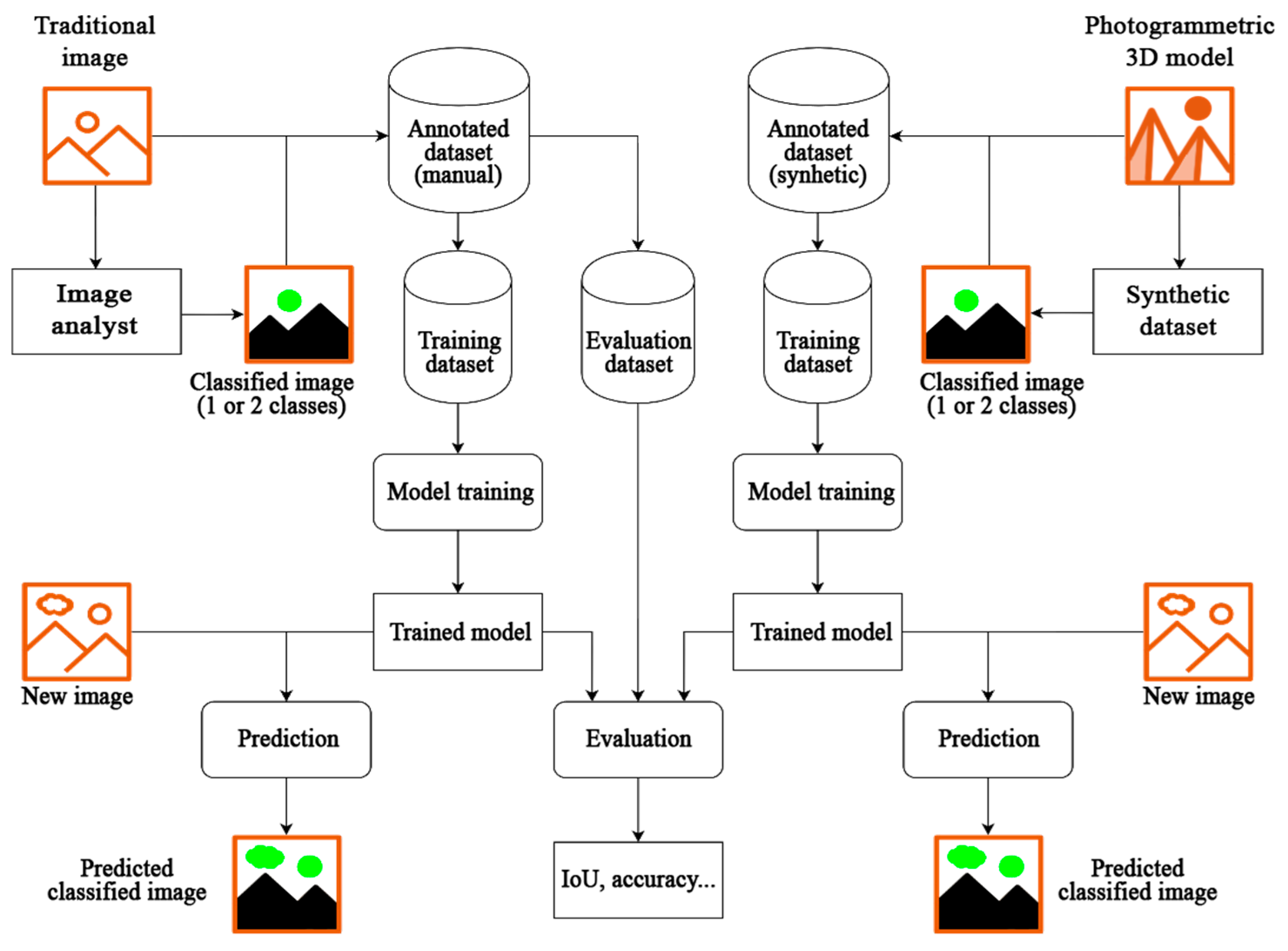
2.1. Research Goals, Aims, and Design

In this research, a flexible methodology for performing image-based classification of cultural heritage at the architectural scale is developed. Specifically, this study focuses on an architectural asset belonging to the 20th-century industrial heritage of industrial concrete, whose conservation is particularly challenging as the relatively recent nature causes a shorter time for the stratification of conservation experiences.

As highlighted in the previous section, this specific type of heritage is exposed to various risks and decay processes, making it crucial to develop methods for automating the monitoring and detection of degradation. Such approaches can effectively support the work of experts in the field of conservation.

This aspect introduces a second objective of the presented research, namely, experimenting with a different type of automatic classification where the task focuses on identifying degradation within the image, in order to perform a decay mapping with an automatic approach, thereby enhancing the sustainability of the process.

Specifically, the structure of the research is as follows:

• A first neural network has been trained using traditional images acquired through traditional methods with the aim of generating a predictive model able to detect the object of interest in the images (single class scenario);
• A second neural network has been trained using synthetic images with the aim of generating a predictive model able to detect the object of interest in the images (single class scenario);
• A third neural network has been trained using synthetic images with the aim of generating a predictive model able to detect not only the object of interest in the images, but also deterioration (multiclass scenario).

For clarity, in the following sections, the first training will be referred to as Training A, while the second and third training—carried out from the synthetic datasets—will be referred to as Training B and Training C.

The architecture used for the presented research experience is DeepLab V3+ [27,28]. Nowadays, there are numerous specific architectures for image classification and semantic segmentation tasks. In the preliminary phase of this research, the authors conducted initial tests using different architectures (such as the well-known U-Net [29] and FC-DenseNet [30]). However, since the main focus of this contribution is not to compare different architectures but to stress the use of synthetic images for degradation identification, the results obtained with the architecture that proved to be most effective in terms of performance, namely DeepLab V3+, will be presented.

DeepLabV3+ is the most recent architecture belonging to the DeepLab family of convolutional neural networks designed for semantic segmentation of images.

DeepLab models employ a backbone architecture, like the well-known ResNet or MobileNet, and combine it with key operations that allow for state-of-the-art results:

• Dilated (Atrous) Convolutions, which allow the capture of information at various scales, thus preserving the details while enlarging the receptive field.
• Atrous Spatial Pyramid Pooling (ASPP), which employs parallel convolutions at different rates, improves the segmentation accuracy.

More specifically, the network architecture is the following:

• The chosen backbone network extracts the features from the input image;
• The Dilated Convolutions and the ASPP are applied to the extracted features to extract multi-scale context;
• The processed features are upsampled to match the original resolution;
• The upsampled features are used to classify the pixels and generate the final segmentation map.

The most recent model, DeepLabV3+, replaces the simple upsampling of the previous ones with a decoder that allows for improved segmentation, especially on object boundaries. The result is the Encoder-Decoder architecture that is widely used in semantic segmentation, which incorporates the aforementioned operations.

DeepLab models proved to be effective at capturing fine details on high-resolution images. More specifically, the improvements brought by these models include higher accuracy in pixel-wise segmentation, better segmentation of small objects and object boundaries, and good performance in challenging scenarios, like urban or medical images. The performances of the network were measured on standard benchmarks like PASCAL VOC 2012 and Cityscapes, achieving better results than other state-of-the-art models like PSPNet and ResNet [28].

In Figure 1, it is possible to observe the flowchart of the proposed workflows. As schematised in the figure, the workflow involves training a predictive model using a training dataset acquired and annotated with traditional techniques (digital images captured with a DSLR camera and manually annotated). A second predictive model was then trained using artificially generated images derived from a photogrammetric model with a high-resolution texture. The performance of both models was compared to assess the suitability of this second strategy in a real-world scenario. Additionally, regarding the approach based on synthetic images, a second case was considered, in which a more complex classification was attempted, aiming at the recognition of exposed iron on the surface of the concrete arch.

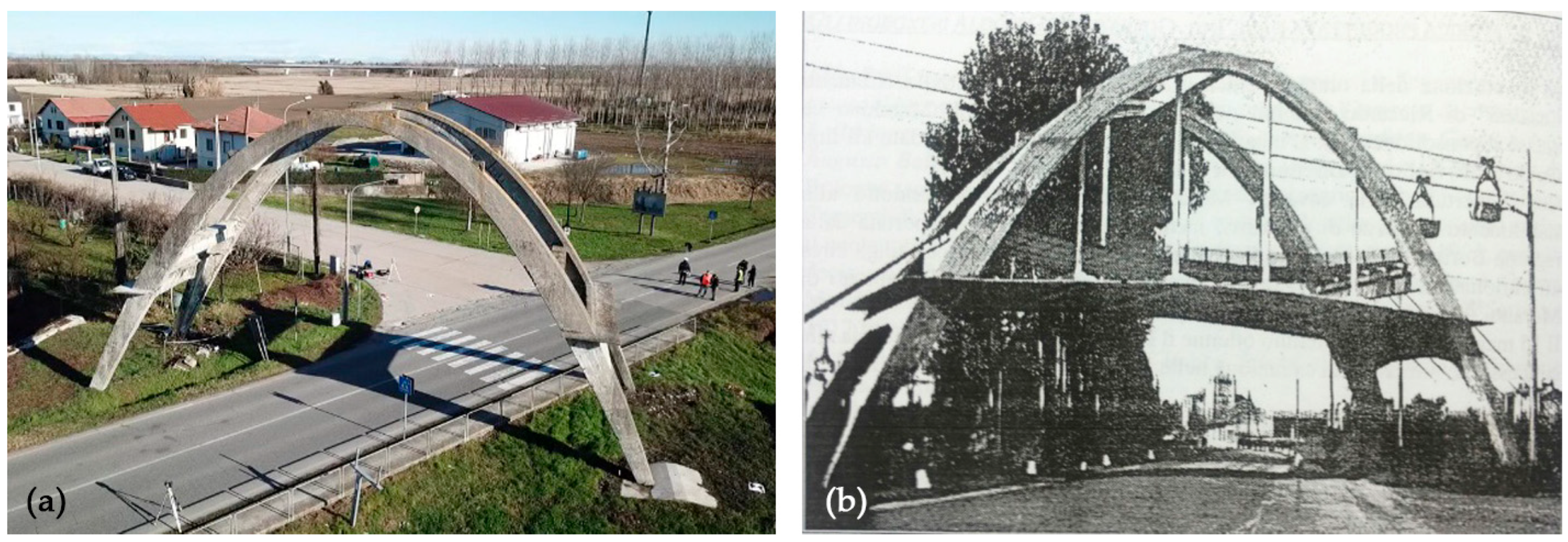
2.2. Case Study: The Parabolic Concrete Arch of Morano Sul Po

Among the many challenges in the conservation field, the management of degradation in 20th century reinforced concrete structures is particularly critical. These buildings, often overlooked in terms of conservation, suffer from deterioration processes that compromise both their structural integrity and cultural value. The 2017 ICOMOS document (Approaches for the conservation of twentieth-century cultural heritage: Madrid—New Delhi Document 2017) [31] emphasises the need for innovative strategies to safeguard 20th century concrete heritage. This concept is also reiterated in the 2022 ICOMOS document (The Cádiz document—InnovaConcrete Guidelines for the Conservation of Concrete Heritage) [26], which places a specific focus on concrete heritage. This highlights the need to develop new, efficient methodologies for decay monitoring. As highlighted in the previous paragraph, from this perspective, supervised methods can represent a significant opportunity to accelerate and automate these processes. In recent years, numerous researchers in the field of Geomatics have carried out studies and investigations on this topic, providing valuable support for the digital documentation of this particular type of heritage [32,33]. Additionally, numerous studies have been conducted to develop systems capable of automatically identifying various forms of degradation, such as cracks [34,35,36].

Regarding the specific case analysed in the present contribution, the case study examined in this research is the Arco di Morano (Figure 2a), a parabolic arch made of reinforced concrete dating back to the 1950s (Figure 2b). Historically, it is an industrial structure linked to the cement production industry, primarily designed to prevent materials from falling onto the road below during transportation—using a cableway—from the Coniolo quarry to the Morano furnace.

This arch represents an important historical and cultural legacy to the industrial production typical of the area. For this reason, in recent years, a conservation plan was developed to preserve the arch, which had fallen into a state of deterioration, with the goal of planning restoration activities and rehabilitating the structure. Therefore, the Polytechnic University of Turin carried out a 3D metric survey, integrating terrestrial LiDAR techniques with digital photogrammetry [37], and performed a series of non-invasive diagnostic investigations to monitor the structural health of the arch [33]. Specifically, in the framework of the 3D metric survey activities, the photogrammetric approach involved the acquisition of high-resolution images both through a terrestrial close-range method and using a UAV system to collect images from above, with the goal of capturing the surfaces of the arch’s intrados. The images belonging to the photogrammetric block, consisting of 606 images acquired as described in the following section, represent the primary data for the composition of both the training dataset and the evaluation dataset.

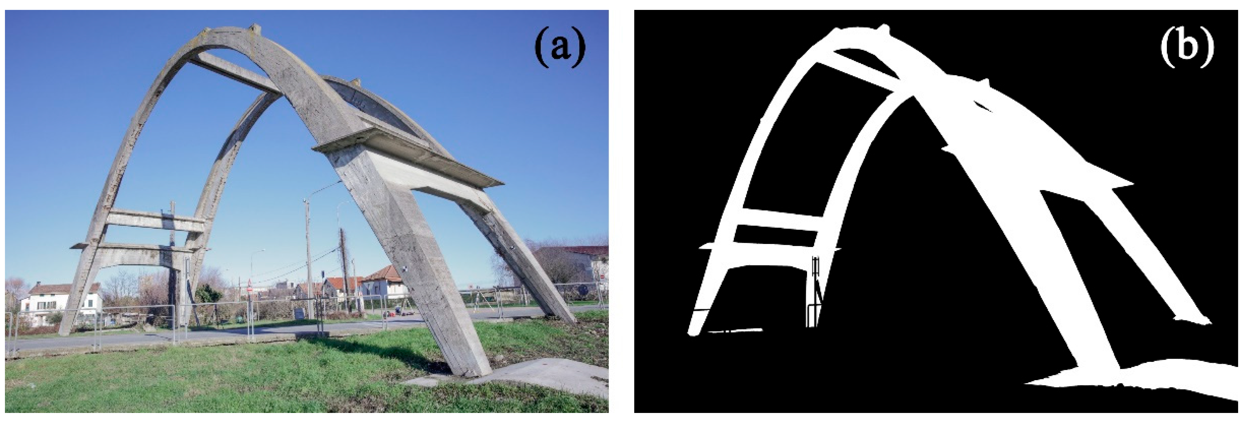
2.3. Primary Data Acquisition and Generation of the Training Dataset (Manual Approach)

During the presented investigation, one of the main aims was to evaluate if the approach presented by the authors in Patrucco & Setragno 2021 [38] and later further developed in Patrucco & Setragno 2023 [25] could be suitable not only for small objects—as in the previous research experiences where the proposed strategy was applied to a collection of wooden maquettes—but also for buildings and architectural scale objects. Additionally, another aspect was investigated concerning the possibility of recognising not only the considered architectural object within a raster dataset but also assessing whether the proposed method is capable of mapping certain types of deterioration.

The results obtained in the previous research experiences are promising, but several aspects affecting the feasibility of this approach should be considered: for example, the impossibility of modifying the acquisition conditions (e.g., the illumination, the background, etc.). If, in the case of the maquettes, the illumination was constant and homogenous, the same condition cannot be guaranteed for the acquisition of the parabolic arch due to the natural illumination. In fact, while it is possible to modify the background (for example, by setting up a green screen) [39] and adjust other factors potentially affecting the acquisition of the images during the digitisation procedures of a movable heritage asset, managing the acquisition environment is significantly less flexible when surveying an architectural-scale object. The critical aspects in this case are twofold. Firstly, in built assets such as the parabolic arch, the background is a predominant element in the images due to the slenderness of the infrastructure. In this sense, it is comparable to bridges, which are high-risk infrastructure elements, particularly those made of reinforced concrete. Secondly, the background contains urban elements that, in terms of characteristics and materials, are entirely similar to the element of interest. This is a crucial issue since, in the case of the concrete arch, in the background are present several elements characterised by similar radiometry or material consistency of the object of interest (e.g., the roads, the sidewalk, concrete elements of the surrounding buildings, etc.). This is one of the reasons why this test has been carried out, i.e., to evaluate the suitability of a deep learning-based approach—for classification and semantic segmentation purposes—in a more complex and less flexible context.

In this case, the digital images used as input data for the neural network training have been collected during a 3D metric acquisition campaign carried out in 2019. As described in Patrucco et al., 2021 [37], photogrammetric acquisition has been performed to acquire the concrete structure. Collectively, 606 images have been acquired: 222 images have been acquired using a DSLR camera equipped with a 25 mm lens (model: Canon EOS 5DSR by Canon, Tokyo, Japan. The main specifications can be observed in

Table 1. Canon EOS 5DSR principal specifications.

Canon EOS 5DSR
Sensor	50.3 [MP]
Sensor size	Full frame, 36 × 24 [mm]
Image size	8688 × 5792 [pixels]
Pixel size	4.14 [μm]
Focal length of used lens	25 [mm]
Used lens model	Zeiss ZE/ZF.2 Distagon T* 25 mm f/2
ISO Range	50–12,800
Shutter speed	30″—1/8000 s

), while 384 images have been collected from a UAV system (model: DJI Mavic Pro by DJI, Shenzhen, China. The main specifications of the UAV system embedded camera can be observed in

Table 2. DJI Mavic Pro camera principal specifications.

DJI Mavic Pro camera
Sensor	CMOS 1/2.3″
Effective pixels	12.35 [MP]
Image size	4000 × 3000 [pixels]
Pixel size	1.53 [μm]
Lens	F/2.2, FoV 78.8° 5 mm (35 mm Equivalent: 26 mm)
ISO Range	100–1600
Shutter speed	8–1/8000 s

) following photogrammetric criteria (ensuring both high overlapping and high convergence of the cameras).

The images have been processed as follows, according to a consolidated photogrammetric workflow [40]:

-

Interior orientation and relative orientation using Multi View Stereo (MVS) and Structure-from-Motion (SfM) techniques;

-

Absolute orientation (for this reason, a set of 28 points was measured using a total station);

-

Accuracy evaluation (for this reason, a second set composed by 6 points was acquired);

-

Depht maps generation and dense point cloud generation;

-

3D mesh generation.

The RMSE (Root Mean Square Error) observed on the GCPs (Ground Control Points) and the CPs (Check Points) after the bundle block adjustment is reported in

Table 3. Accuracies observed on GCPs and CPs.

	X [m]	Y [m]	Z [m]	XYZ [m]
GCPs [28]	0.006	0.006	0.008	0.012
CPs [6]	0.009	0.004	0.009	0.013

.

It should be underlined that a preliminary manual masking procedure was necessary to orient the image properly, selecting the pixels of the disturbing elements in the background potentially affecting the autocorrelation case—e.g., sky, vegetation, moving elements, etc.—and excluding them from the photogrammetric process. Without this procedure, orienting the entire block of images would not be possible. Obviously, this criticality does not exist in many heritage cases, when the object of interest occupies almost the entire percentage of the image. Additionally, the following strategy has been followed to optimise the quality of the exclusion masks that shall be used as labels for the subsequent training procedure. Firstly, after the generation of the dense point clouds, a 3D mesh was generated. The mesh was then segmented, removing all the elements except the concrete arch (e.g., the road, the sidewalk, etc.). The segmented 3D surface has been subsequently reprojected on the oriented images—exploiting the “Import masks from model” tool implemented in the Metashape (v. 1.8.0) platform—creating the .png labels necessary for the neural network training. In some cases, some manual corrections have been necessary to solve some issues due to mesh topological errors and mis-projections. This aspect related to the automation of masking procedures represents an undeniable challenge in the effort to streamline the costly and time-consuming processes associated with heritage digitisation. Also in this case, a possible solution involves the use of ML and DL approaches, and in this regard, several studies have been carried out in this direction [38,41].

At the end of this procedure, the dataset is composed of 606 digital images, and the corresponding .png masks are used as labels to identify the object of interest. In Figure 3, it is possible to observe the original image (Figure 3a) and the exclusion mask (Figure 3b), identifying the pixels belonging to the object of interest.

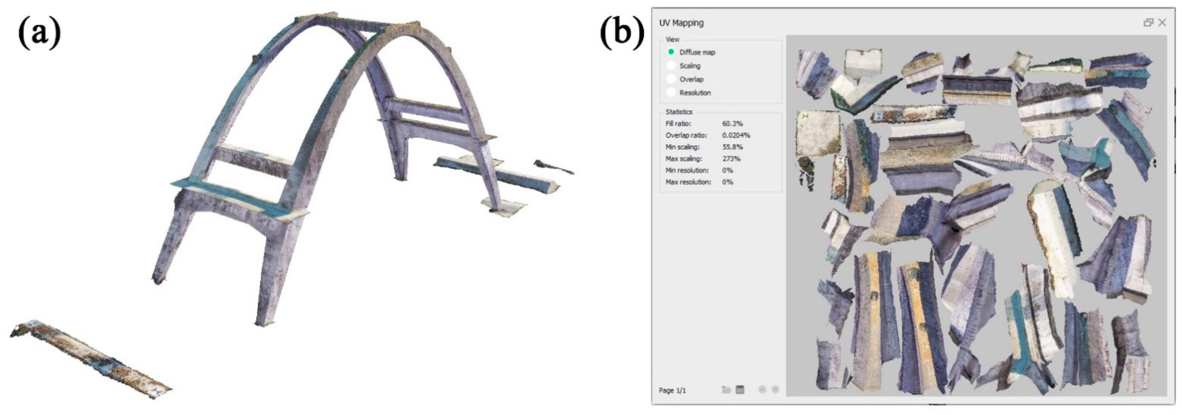
2.4. Generation of ‘Synthetic’ Training Datasets from Photogrammetric Models

In this section, a methodology to automatically generate a synthetic training dataset is proposed, exploiting digital photogrammetry. As previously referred, 3D models achievable from photogrammetric techniques are characterised by high spatial and radiometric resolutions. Exploiting these two aspects of the three-dimensional models that nowadays we are able to achieve can represent a possibility for the generation of artificial datasets characterised by adequate features for the training of a neural network.

Specifically, as specified in Section 2.1, both 1-class scenario and 2-classes scenario will be described, evidencing the potentialities of this method not only for the automatic recognition of the pixels belonging to the object of interest but also considering more complex tasks like automatic classification of decay and degradation. Namely, in the specific framework of this research experience, the automatic detection of exposed iron has been considered, as introduced in Section 1.

Starting from the high-resolution textured 3D model of the parabolic arch of Morano, a synthetic dataset of rendered images will be generated and used for training a neural network, employing the same strategy and the same parameters described in the previous section. The performances will be compared with the results obtained from the previous training, where traditional images have been used as input dataset, to evaluate if artificial images—generated using this approach—can represent an adequate alternative for training a neural network.

2.4.1. Single Class Scenario

The first considered task consists in the automatic generation—and labelling—of a dataset of artificial rendered images derived from a textured 3D model.

A 3D triangular mesh was generated starting from the dense cloud derived from the SfM photogrammetric approach described in Section 2.3. The generation of this triangular mesh was carried out using the algorithm implemented in the photogrammetric platform employed (Agisoft Metashape v. 1.8.0). The achieved 3D model is composed of ca. 500,000 faces (Figure 4a). Additionally, a high-resolution UV map was also generated (resolution: 8000 × 8000 pixels) to provide a texture to the model (Figure 4b), and therefore information about radiometry and material consistency. UV mapping is a texturing technique enabling the projection of a 2D image—the so-called UV map—on the surface of a 3D model. In this case, the UV map has been generated from the oriented images of the photogrammetric block through orthorectifying and mosaicking procedures. For each point of the 2D textured surface located in a UV space, the three-dimensional position of a vertex of the 3D mesh is assigned, enabling the projection of the texture. In this case, U and V represent the Cartesian axes of this two-dimensional reference system, while the 3D model is located in an XYZ reference system [42,43].

The textured 3D model has been exported from the Metashape software in COLLADA file format (.dae). The selected file extension includes the information related to the camera position and assets of the cameras, which will be used to create the artificial images dataset. The model was subsequently imported in the open-source software Blender v. 2.93.1, which is able to read the information about the oriented cameras and use them as virtual camera for the generation of the rendered images (Figure 5).

A Python 3.9 script was used to automatically generate rendered images of both models, exploiting the oriented cameras—exported from Metashape and used as virtual cameras by the Blender platform—in order to generate the artificial images and the corresponding labelled images. The used script can be observed in Figure 6.

According to this strategy, it was possible to generate 606 rendered images. The resolution of the images is the same as the original ones: 8688 × 5792 pixels for the images acquired from the DSLR camera and 4000 × 3000 pixels for the images acquired from the UAV system embedded camera. In order to facilitate the automatic generation of the labels, two different models have been used:

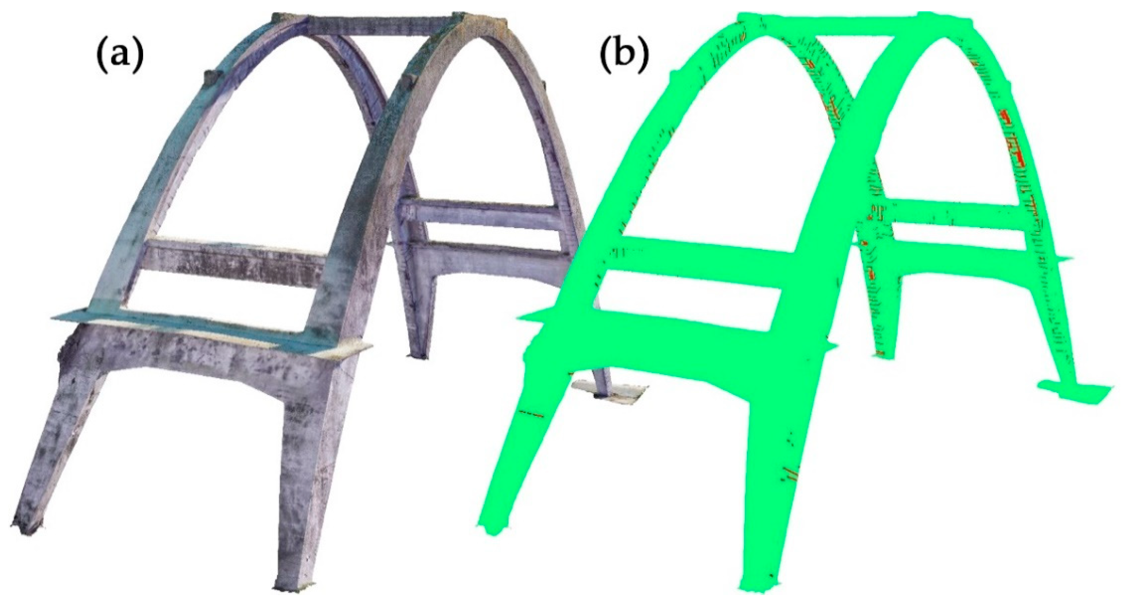
• The 3D mesh of the arch with the context (road, vegetation, sidewalk, etc.) for the generation of the rendered images. Regarding the training dataset, the context can provide some learning features (e.g., radiometric features of elements belonging to the background, geometric features, etc.) useful for the neural network training.
• The 3D mesh of the arch without the context (in this case, every element except the arch has been manually deleted, to facilitate the automatic extraction of the labels).

The synthetic dataset has been generated from the first 3D mesh (Figure 7), while the second—segmented—mesh has been used to generate the labels by subtracting the pixels belonging to the background, automatically identified—using a script—according to an RGB-based selection, made possible by the possibility of modifying the virtual background of the textured model in the Blender platform to facilitate the automatic generation of the annotated labels (Figure 8). This strategy—of course—would not be applicable to datasets composed of traditional digital images acquired by camera sensors, since in that case the background is not characterised by a single RGB value and therefore the RGB-based selection strategy would not work.

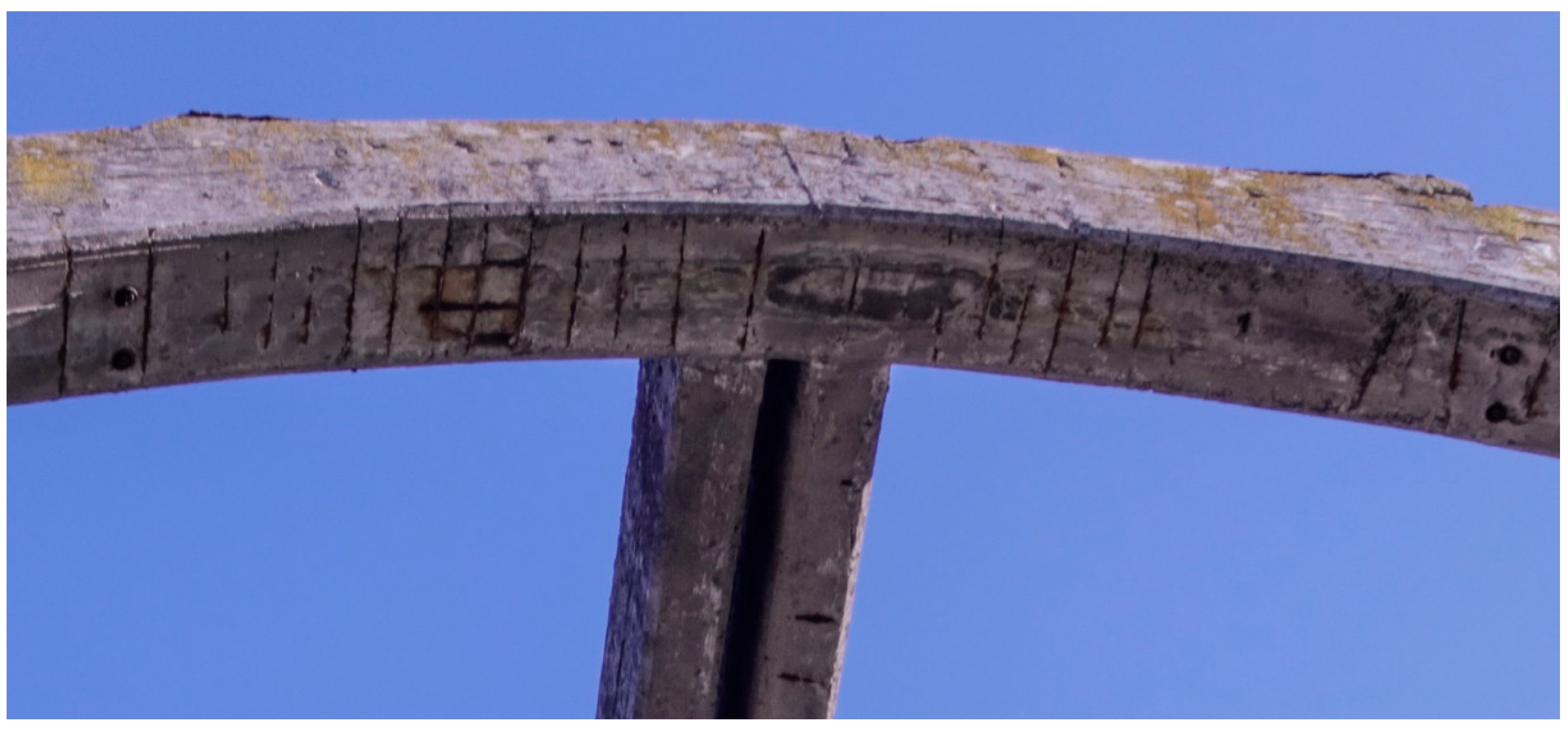
2.4.2. Multi-Class Scenario: Concrete Degradation Detection

The second carried-out experiment regards the possibility of performing a multi-class segmentation starting with synthetic data generated following the methodology described in the previous paragraph. In this case, the aim of the test is not only the automatic identification of the object of interest (the arch) but also the detection of the concrete degradation. Specifically, in the proposed case, the exposed irons affecting the surfaces of the arch—in particular in the intrados—have been considered (Figure 9).

This second task is far more complex in comparison to the first one, due to the introduction of a new class (the degradation of the exposed iron) and the lack of homogeneity between the classes (the class of the exposed irons is significantly smaller compared to the background class and the concrete arch class, occupying a significantly lower portion of pixels).

The proposed workflow is as follows:

-

Mesh generation;

-

UV map generation for texture mapping;

-

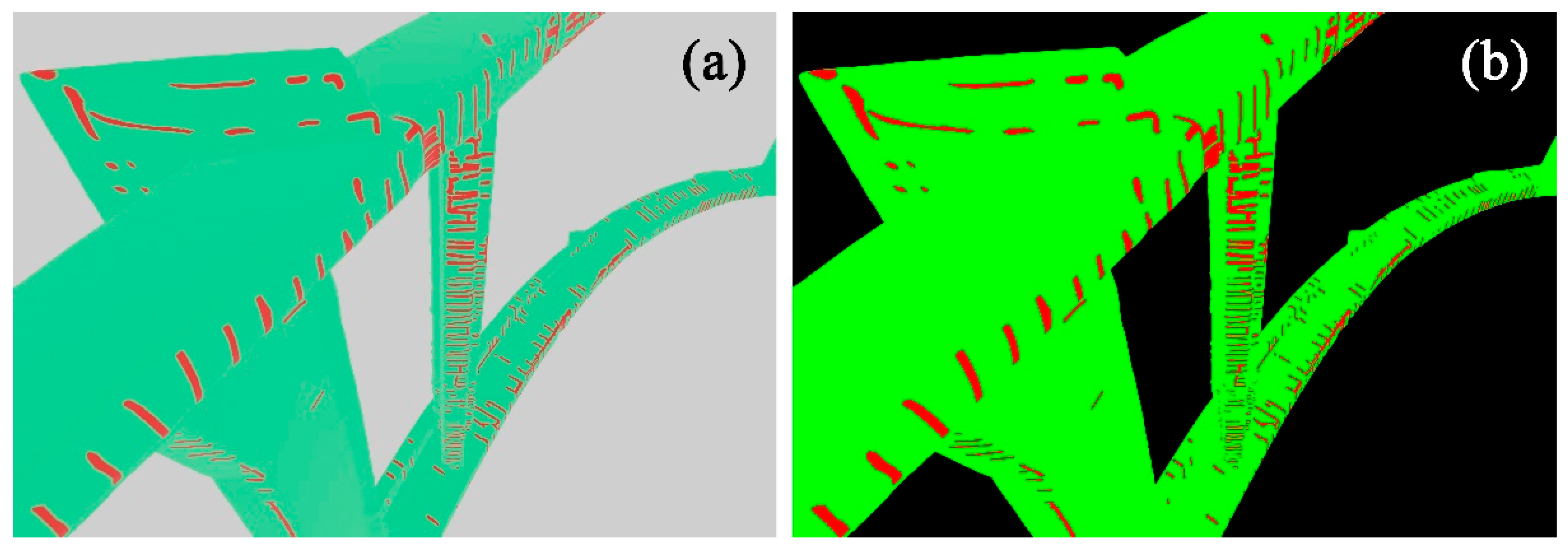
Manual (multi-class) segmentation of the UV map (the segmented classes are: 0—background, 1—concrete, 2—exposed iron);

-

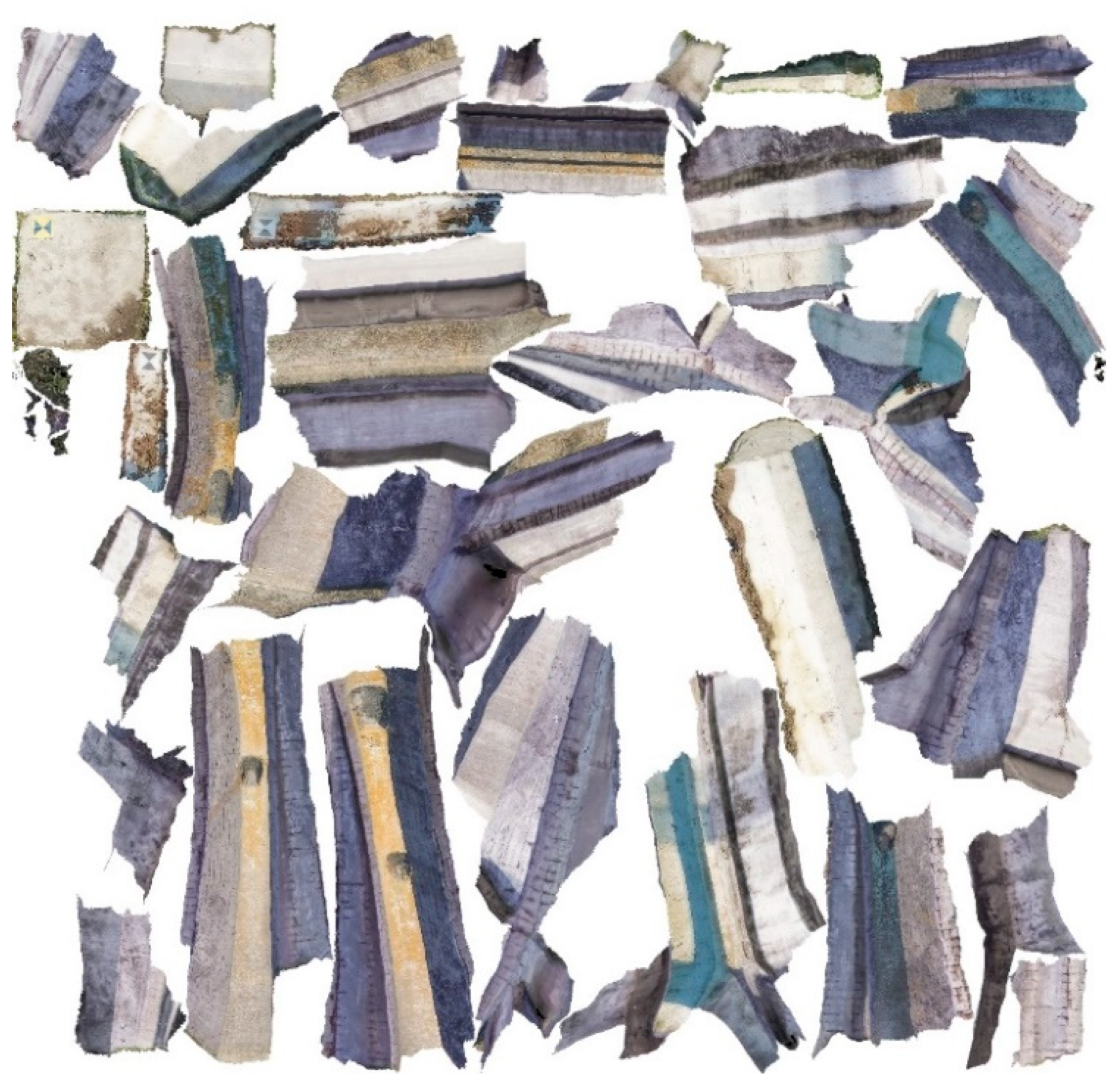
Reprojection of the classified texture;

-

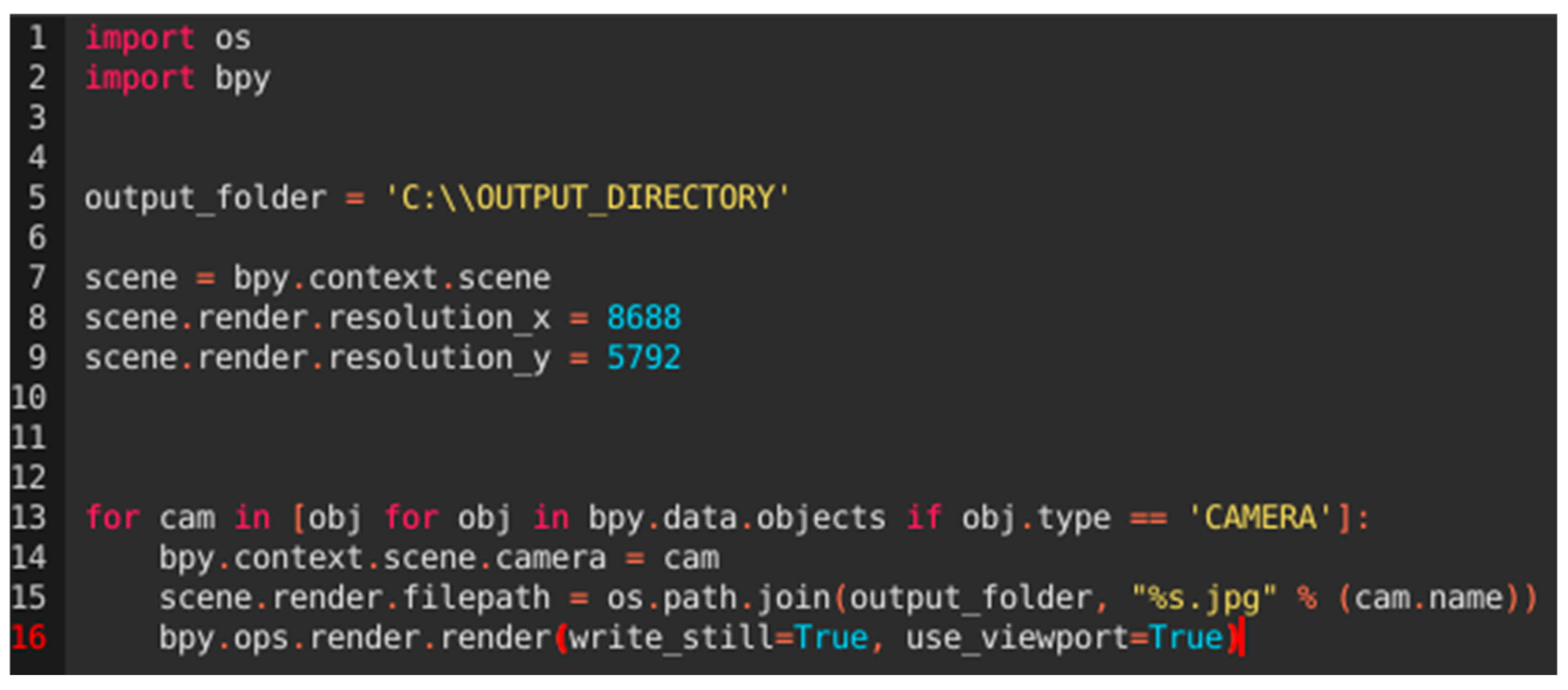
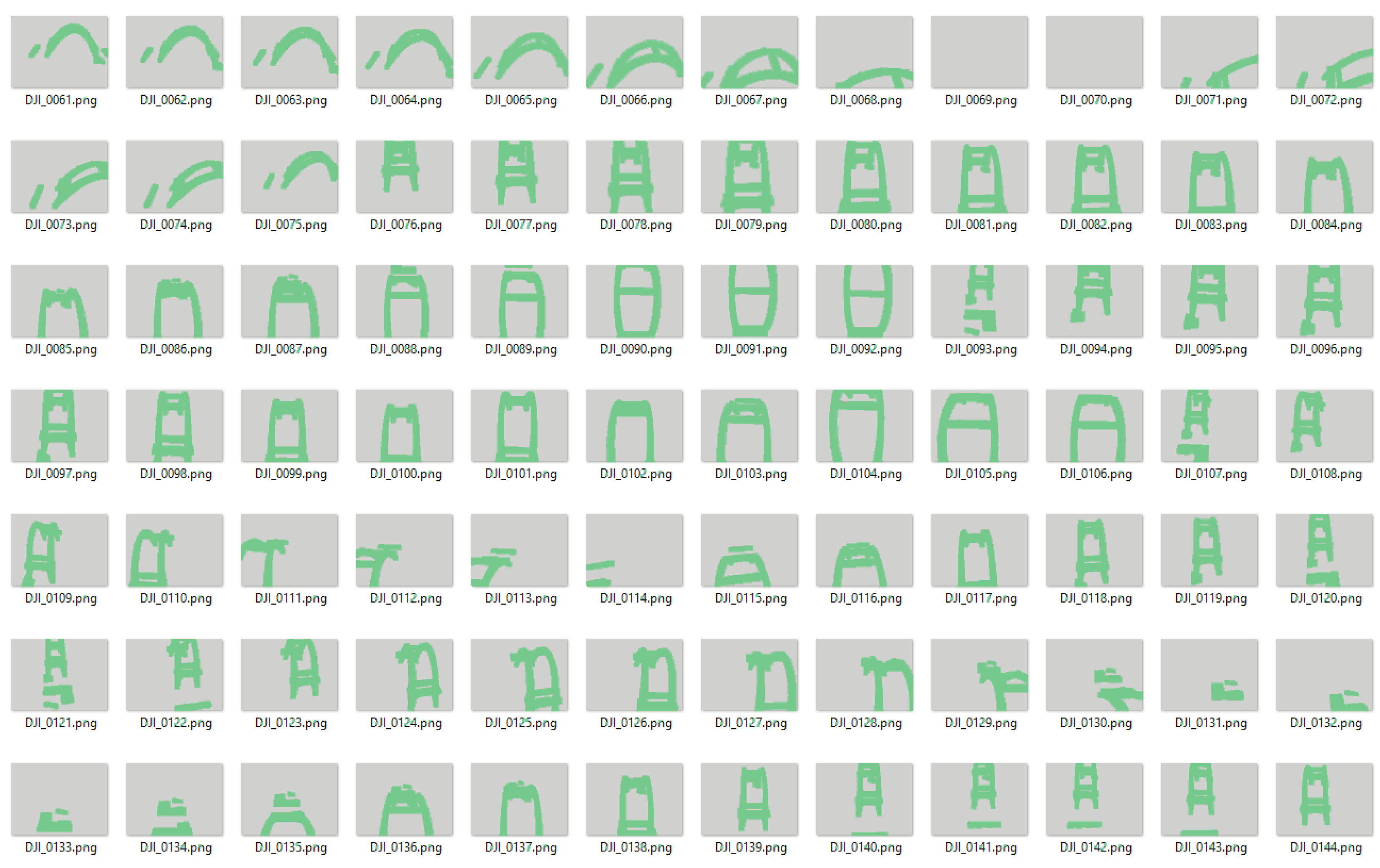
Automatic generation of the synthetic rendered training dataset;

-

Automatic generation of the rendered multi-class labels;

-

Reclassification procedure to convert the rendered multi-class labels into a properly formatted ground truth for the training;

-

Neural network training (the training will be referred to in the next paragraphs as Training C).

As in the previous case, the starting point is the generation of a 3D triangular mesh and, subsequently, the generation of a high-resolution UV map. The parameters are the same as the previous test (mesh faces ca. = 500,000; UV map resolution = 8000 × 8000 pixels). The UV map generated after the texture mapping has been exported (Figure 10) and manually classified using image editor software (Adobe Photoshop v. 23.5.5). The manual procedure required ca. 30 min, during which all the identified exposed iron was mapped. The final result of this operation can be observed in Figure 11 (white = background; green = concrete; red = exposed iron).

The UV map was then reprojected on the 3D model mapping the classified exposed irons on the 3D surface (Figure 12).

After importing the model in Blender (format: COLLADA, .dae), the artificial dataset has been generated following the procedure described in the previous section. This operation was carried out for both the true colour textured 3D model for generating the artificial training imagery and the classified texture 3D model for the classified annotated labels. However, in this second case, a further raster reclassification procedure was necessary to adapt the generated labels in order to convert them into a properly formatted ground truth for the training. The pixels generated images contain more than three digital numbers while, after the aforementioned processing, the classified label raster images contain only three pixel values: 0 for the background, 1 for the concrete parts of the arch, and 2 for the areas characterised by the presence of exposed iron (Figure 13).

2.5. Neural Network Training

This section describes in detail the process of training the neural networks for the three mentioned tasks, including data pre-processing and hyperparameter choice.

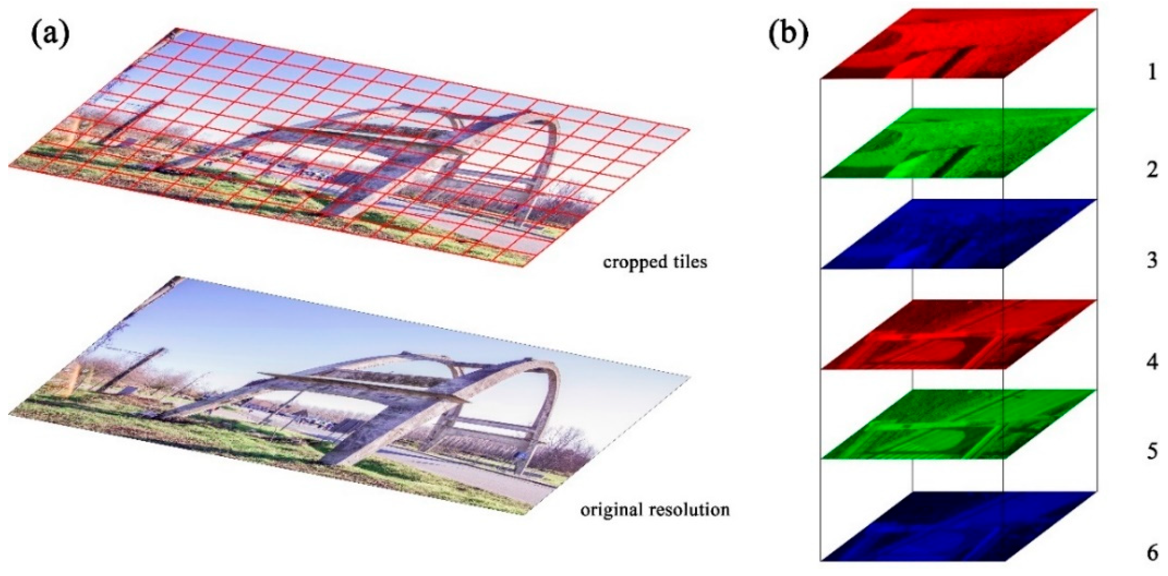
2.5.1. Dataset Preparation

The dataset was built by applying the following strategy to the high-resolution images. With the aim of improving the performance of the training, avoiding out-of-memory errors due to the excessive resolution of the employed images (resolution of the images acquired with the DSLR camera = 8688 × 5792 pixels; resolution of the images acquired with the UAV system = 4000 × 3000 pixels) and, at the same time, exploiting the original high spatial resolution—and therefore the high level of detail—of the collected datasets, each digital image has been divided into different tiles (512 × 512 pixels) rather than just downsampling the images. However, to ensure that the network could learn features from the contextualisation of each tile, a subsampled version of the original image has been added to the cropped tiles, generating a multiband raster.

Every image of the training dataset is therefore characterised by a resolution of 512 × 512 pixels, and it is composed of 6 bands:

-

First band: cropped tile (original resolution), Red band;

-

Second band: cropped tile (original resolution), Green band;

-

Third band: cropped tile (original resolution), Blue band;

-

Fourth band: downsampled image, Red band;

-

Fifth band: downsampled image, Green band;

-

Sixth band: downsampled image, Blue band.

The scheme of the band composition applied for the generation of the multi-band raster images used as input training dataset can be observed in Figure 14.

Following this strategy, it is possible to exploit the high level of detail of the high-resolution digital images without loss of information derived from the downsampling (leading to a more detailed exclusion mask); at the same time, the neural network learns from the contextualisation of each tile. However, this affects the computational efforts required for the training since in this way the dataset is divided into more than 60,000 images with 6 bands rather than 3, with a consequent increase in the computational effort and processing time required for the training.

For this reason, as underlined in Section 2.1, the deep network architecture used during this research experience is the well-known DeepLab V3+ architecture [27,44], allowing for effective management of a larger amount of data.

2.5.2. Data Augmentation

Nowadays, to enhance training performance despite the limited number of images used as a training dataset, it is a well-established practice to employ data augmentation techniques [45]. In the case described in the current research, the following consolidated data augmentation techniques have been applied:

• Random brightness change: the brightness of the image is randomly changed by uniformly increasing/decreasing the pixel values up to ±10 (with pixel values going from 0 to 255 on unsigned 8-bit integers);
• Horizontal flip;
• Random rotation: the image is rotated with a random angle up to 30°. The resulting blank areas are filled using the nearest neighbour interpolation;
• Random background change: the pixels labelled as background are replaced with a random image;
• Random occlusion: a square of random side (up to 30% of the image side) is filled with black at a random position.

During the training, each time an image is loaded, a random combination of these techniques is applied, each with a 50% probability.

2.5.3. Model Training

During the training, batches of images are loaded, preprocessed using the abovementioned augmentation techniques, and fed to the neural network. The optimisation algorithm computes the training loss and updates the weights of the network. The validation accuracy is periodically computed on the validation set (see Section 3.1.1) and compared to the training accuracy in order to ensure that the model is not overfitting.

The combination of training hyperparameters used is reported below, selected based on the best performance across the various tests carried out.

Every training is performed using a learning rate of 0.001, a batch size of 32 images, 100 epochs, and a dropout rate of 20%. The learning rate was decreased during the training using an exponential decay with a rate of 0.99 every 1500 training steps. The optimiser algorithm was Adam [46].

3. Results

3.1. Generation of the Predictive Models

Starting from the different datasets generated as described in the previous section, three neural networks have been trained as described in the following sections.

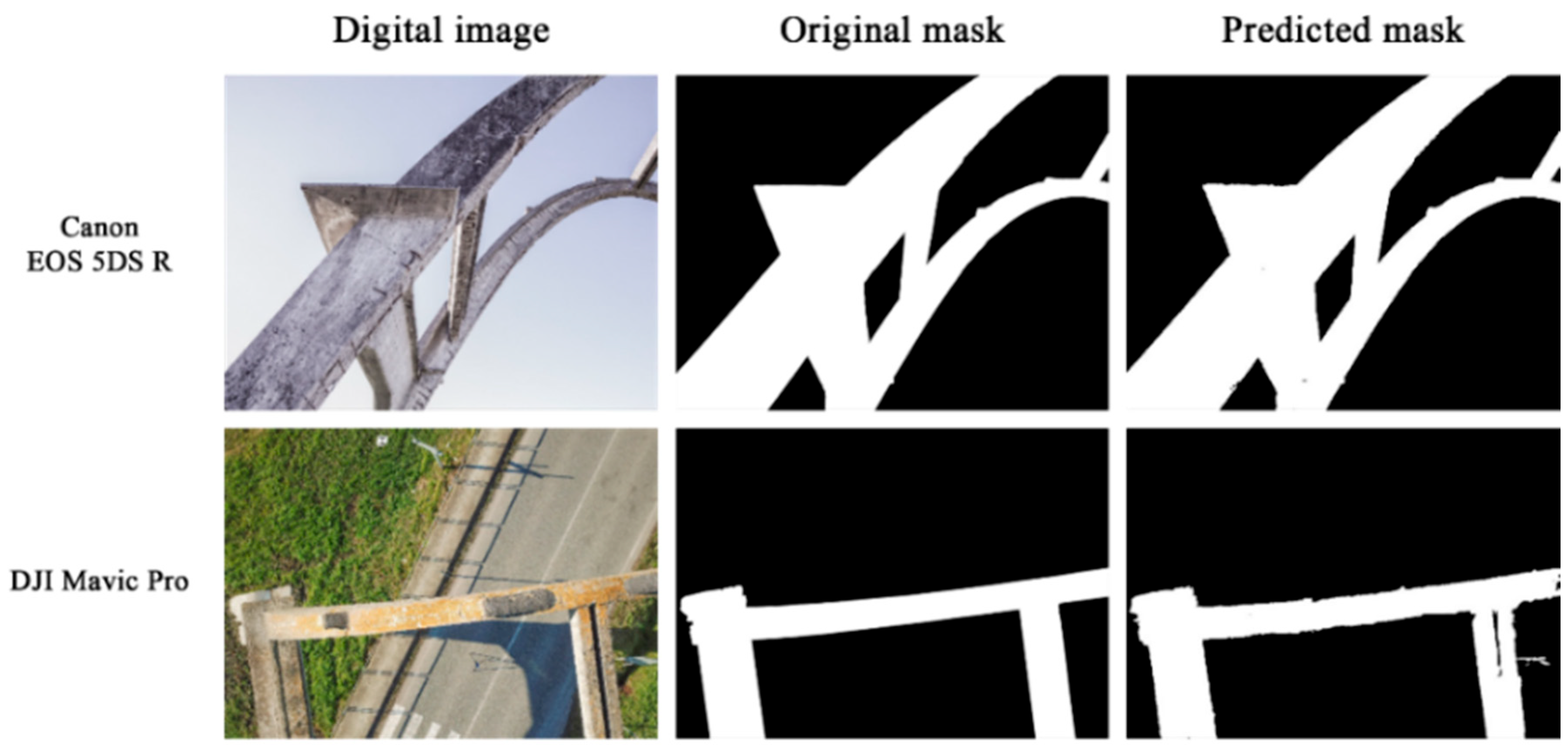
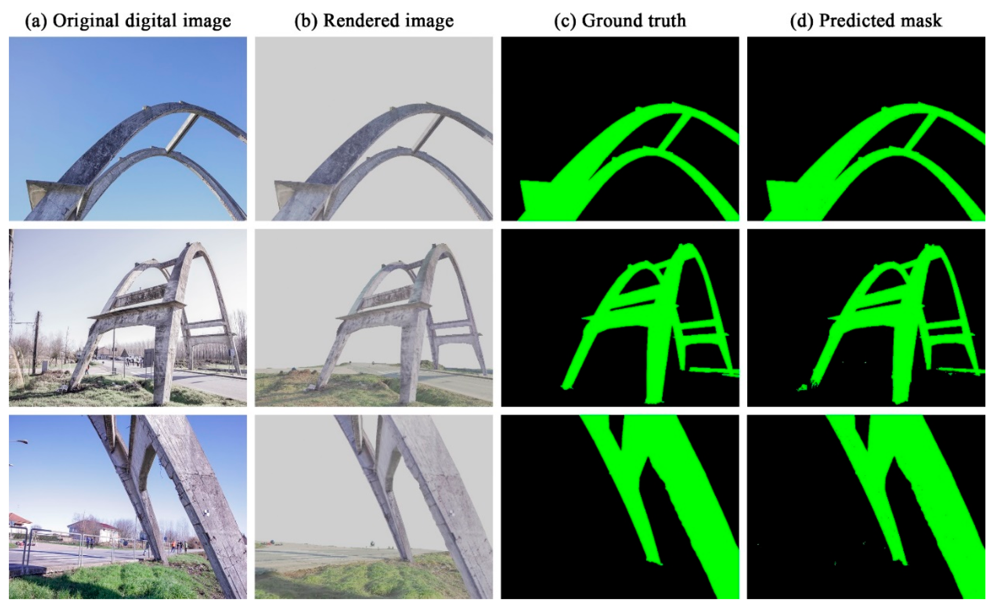
3.1.1. Neural Networks Training Using Synthetic Dataset (Single Class Scenario)

In the first case (Training A), the neural network was trained to classify the concrete arch as Class 1 and the background as Class 2. The dataset was split into a training set and a validation set, with the purpose of measuring the accuracy of the trained model. Typically, the empirical 80-20 rule is employed (80% for the training set and 20% for the validation set) in order to ensure that the validation set is sufficiently representative of the whole data distribution. However, in this case, the amount of available data was particularly low for this task, and we could not afford to devote many images to the validation. We tried to reduce the validation set, and we found that a 90-10 proportion performed well. This means that 545 randomly selected images were used for the training and 61 for the validation. While it is true that a higher percentage of validation images allows for better identification of overfitting during the training, we managed to do it by constantly monitoring and comparing the training and validation accuracy during the process. Furthermore, the dropout regularisation technique was applied to reduce the risk of overfitting [47]. This aspect was also considered in the subsequent training processes carried out throughout this study.

As in the previous case, for each image, a homologous labelled mask has been used as ground truth, assigning to each pixel a value corresponding to a specific class (in this case: 0 for the background, 1 for the pixels belonging to the concrete arch). The same script previously used for the wooden maquette has been used to convert the .png masks into a properly formatted ground truth.

The following performance evaluation metrics have been used to assess the quality of the neural network performances after training: Accuracy, Mean IoU, Precision, Recall, and F1-score. These measures were calculated using the validation dataset composed of the images not involved in the neural network training procedures. The obtained results are reported in

Table 4. Performance evaluation metrics of the neural network training.

	Training A (Traditional Digital Images)
Accuracy	99%
Mean IoU	92%
Precision	97%
Recall	99%
F1-score	98%

. As it is possible to observe, the overall quality of the training—evidenced by the achieved results—demonstrates that, despite the bottlenecks described at the beginning of this section, the performances of the trained neural network are adequate compared to the required task and that the used approach is sufficiently flexible not to suffer the influences of external disturbing features (e.g., not homogenous illumination, the presence of elements characterised by similar radiometry and material consistency of the analysed case study).

In Figure 15, it is possible to observe a visual comparison between the original digital image used as input primary data for the training, the original mask used as annotated ground truth, and the predicted image. The comparison has been performed using images acquired by the DSLR camera and the DJI Mavic Pro embedded camera. From a visual inspection, it can be noticed that the masks predicted from the DSLR camera images are those characterised by the best quality, but also the masks derived from the DJI Mavic Pro embedded camera images have been adequately generated, despite the presence of some topological errors and little clusters of misclassified pixels.

Also, in this case, a qualitative evaluation of the generated exclusion masks has been performed, using the automatically classified images as exclusion masks during the photogrammetric processing of the concrete arch dataset. The 606 images have been reprocessed using the automatically generated exclusion masks and, as expected—considering the achieved performance evaluation metrics, indicating a proper functioning of the trained algorithm—the results are coherent with the ones obtained using the manually generated masks (in terms of completeness, noise, number of points of the dense point cloud, etc.).

Regarding Training B (training dataset composed of synthetic images; single class scenario), the training procedures and parameters are the same as described in the previous paragraphs. Also in this case, the DeepLab V3+ architecture was used, and the same data augmentation strategies of Training A have been applied. Analogously to the previously mentioned case, the images have been divided into 512 × 512 pixels tiles, to preserve the possibility for the neural network model to learn from the high level of detail of the images, and the information about the contextualisation of the considered tile has been stored in the raster file as additional bands.

As it is possible to observe from the performance evaluation metrics calculated on the evaluation dataset, the obtained results are completely consistent with those achieved from Training A. The achieved metrics are reported in

Table 5. Comparison of Accuracy, Mean IoU, and F1-score between 1 Class training and 2 Classes training.

	Training A (Traditional Digital Images)	Training B (Synthetic Data)
Accuracy	99%	98%
Mean IoU	92%	90%
Precision	97%	96%
Recall	99%	99%
F1-score	98%	97%

.

In Figure 16, it is possible to observe a comparison between the original image (Figure 16a), the rendered image belonging to the synthetic dataset with which the neural network was trained (Figure 16b), the automatically generated artificial ground truth (Figure 16c) and the predicted classified image (Figure 16d).

As in the previous case (Training A), the trained neural network model has performed the pre-established task with a high level of accuracy. The visual inspection and the calculated performance evaluation metrics show that both the strategies followed for Training A and Training B have produced adequate results.

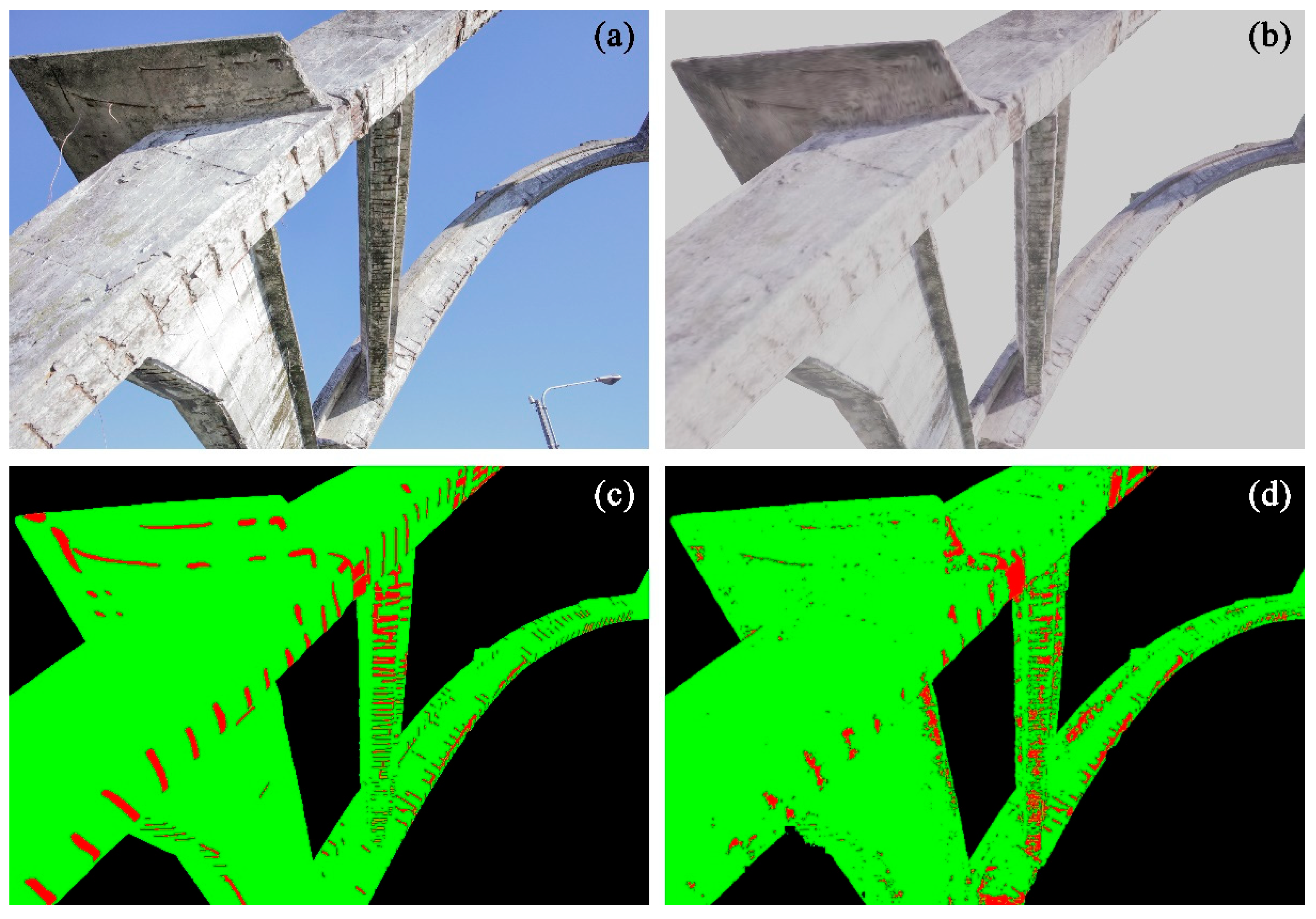
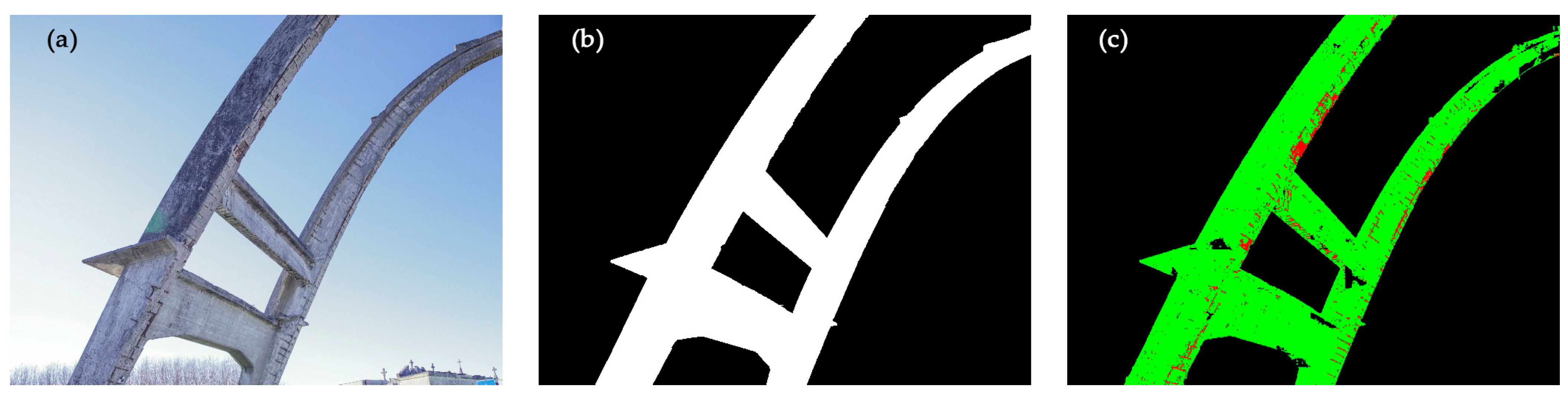
3.1.2. Neural Network Training Using Synthetic Dataset (Multiclass Scenario)

The two datasets have therefore been used for the neural network training, which was performed as described in the previous sections. As expected, Training C was the one characterised by the lower accuracies observed on the calculated performance evaluation metrics. Specifically, Class 2 (exposed iron), due to the aforementioned disparity with the other classes, was characterised by lower metrics—particularly IoU ≈ 55%, evidence of a medium-low performance—caused by the lack of correspondence between the predicted areas and the ground truth (the achieved results can be observed in

Table 6. Comparison of Accuracy, Mean IoU, and F1-score between class 1 (concrete parts of the arch) and class 2 (exposed iron).

	Training A (Traditional Digital Images)	Training B (Synthetic Data)
Accuracy	84%	78%
Mean IoU	82%	55%
Precision	92%	69%
Recall	88%	66%
F1-score	90%	67%

).

This was partially predictable, considering the higher complexity of this task compared to one from the single-class scenario. Additionally, the boundaries of the degraded materials are not characterised by high sharpness, and this characteristic negatively affects the automatic detection due to the difficulty in identifying the exposed iron’s margins.

4. Discussion

Regarding the multiclass segmentation, from a visual inspection (Figure 17d) it is evident that, although the neural network model failed to identify with a high level of accuracy the areas characterised by the presence of the exposed iron, the areas classified as exposed iron correspond to the actual location of Class 2, and therefore the model managed to map the position of the degradation where most concentrated.

The low performance of the network regarding Class 2 affected also the results of the accuracies observed on Class 1; in fact, despite all the metrics being ≥ 80%—and therefore cannot be considered negative in an absolute sense—it should be underlined that in this case the achieved results are significantly lower compared to the ones obtained to the previous trainings (Training A and Training B) where the concrete arch was unambiguously identified with performance evaluation metrics ≥ 90%.

However, despite the non-optimal results obtained from the third training—partially due to the difficulties in unambiguously identifying the borders of the exposed irons—it should be underlined how this last experimental experience can represent a promising first step—and an interesting future perspective—for the implementation of AI algorithms for automatic decay detection in the framework of wide-ranging research in the construction and heritage of the twentieth century.

In

Table 7. Comparison between the results of Training A, Training B, and Training C in terms of Accuracy, Mean IoU, Precision, Recall, and F1-score.

	Training A	Training B	Training C
	Single Class	Single Class	Class 1	Class 2
Accuracy	96%	98%	84%	78%
Mean IoU	92%	90%	82%	55%
Precision	97%	96%	92%	69%
Recall	99%	99%	88%	66%
F1-score	98%	97%	90%	67%

, a summary comparison between the achieved results is observed considering the three different processing carried out in the previous sections: Training A (single class training from traditional digital images), Training B (single class training from synthetic rendered images) and Training C (multi-class training from synthetic rendered images).

One last aspect that deserves to be highlighted regards the usability of the trained algorithms, not only concerning the rendered images—with which the neural networks have been trained—but also considering the possibility to apply the algorithm on “real” images, acquired with camera sensors. In Figure 18, it is possible to observe a digital image of the arch (acquired using a DSLR camera) processed with both the single class and multi-class neural network models trained from the synthetic dataset (Training B and Training C).

From a qualitative perspective, it can be observed that class 2 (exposed irons), although characterised by high noise, has been effectively mapped, as well as class 1 (concrete), highlighting its position on the analysed structure. Another consideration concerns the presence of clusters of pixels erroneously classified as belonging to class 0 (background) on the surface of the concrete arch. This phenomenon is more frequently observed in some shadowed areas (mainly located in the intrados of the structural elements) and in areas characterised by the presence of different types of degradation (e.g., efflorescence, biological patina, etc.).

5. Conclusions

In conclusion, this study demonstrated the promising potential of using synthetic datasets derived from photogrammetric models to train deep learning algorithms for heritage conservation tasks. By applying this methodology to the parabolic concrete arch of Morano sul Po, the study evaluated the effectiveness of synthetic images in both single-class and multi-class segmentation scenarios. As introduced in the Section 2.1, it should be underlined that in the presented case the oriented cameras have been used to evaluate the pros and the cons of the neural network trained with traditional digital images and the one trained with the rendered images, using similar parameters for an objective comparison (same number of images, same FoV, etc.). However, there are several Python scripts—that can be run on Blender—to generate multiple rendered images of a 3D model from random points of view, so it is not strictly necessary to have oriented cameras in the Blender environment. Following this strategy, it would be possible to generate vast amounts of artificial data—potentially tending to infinity—that could contribute to optimising the training procedures, which traditionally require a high number of datasets [48]. The acquisition of massive amounts of data would be very challenging using reality-based techniques, as well as the generation of annotated labels.

Concerning the obtained results, the best performance was observed in single-class classification, as expected, since the task was less complex. In this case, the performance achieved can be considered highly effective, as the difference in terms of metrics between predictive model A and predictive model B is of the same order of magnitude. In the previous research study reported in Patrucco and Setragno 2023 [25], despite the good performance observed for the model trained on synthetic images, there was still a gap in terms of performance if compared with the evaluation metrics achieved by the traditional DL model. This could indicate that the rendered images, although similar to the traditional input images intended for classification, still have differences that affect performance. However, in the case of the concrete arch, likely due to the high specificity and spatial configuration of the object to be segmented, there is almost an equality in terms of performance between the two models. This represents a significant result; nevertheless, it should be underlined that a crucial limitation of the proposed method is that the described strategy is connected to a very specific use case. This represents a limitation since one of the aspects that still remains open for further research is the improvement of the generalisation capability of the trained models, currently limited to recognising homogenous classes of objects characterised by very similar features and appearances, and not feasible for other assets characterised by a more heterogeneous aspect. In fact, while the model trained from the parabolic arch dataset is able to perform the classification task also for structures characterised by similarities in terms of shapes and material consistency (Figure 19), using the same algorithm to process images of concrete heritage assets characterised by different characteristics and morphologic features produce results significantly less accurate (Figure 20). In this second case, the image has been processed using the trained neural network, and the prediction is characterised by low accuracy, although some shape-related features have been properly identified.

This could be due to the fact that, despite sharing a common geometry—both the arch and the vault of the considered building have a parabolic shape—and a similar material consistency, as both are made of reinforced concrete, their morphology differs significantly. In fact, while the object shown in Figure 20 can be considered a building from all perspectives, the slenderness that characterises the concrete arch makes it resemble more of a thin infrastructure or a bridge.

For this reason, it is worth considering the opportunity to build on the generative model obtained through the methods described in the previous paragraphs, extending it to the monitoring of thin reinforced concrete structures—an increasingly relevant topic in the field of infrastructure monitoring.

In fact, processing the image of a bridge (Figure 21) using the single-class predictive model derived from synthetic images (Training B) results in a classification that, while characterised by a high level of noise, is still more consistent than what can be observed in Figure 21.

This aspect is of significant importance, as bridge monitoring is crucial and requires continuous investment, along with the development of specific strategies to make the related operations more automated and sustainable. As underlined, an undoubtedly interesting future perspective to enhance the efficiency of these automatic procedures is represented by the possibility of generating predictive models characterised by high generalisation capability or, alternatively, adapting pre-existing predictive models using transfer learning techniques and fine-tuning. In this specific case, by applying fine-tuning procedures or refining the outcome with pre-trained models—such as the well-known SAM [17], which has been increasingly used for similar purposes in recent times—it may be possible to generalise the proposed method and improve its generalisation capability. In both cases, the possibility of generating synthetic datasets could be a valid strategy to pursue this direction, representing an opportunity with significant impact. An important future research direction for the authors involves the identification of pre-trained models capable of performing tasks comparable to those presented in this paper. This would allow for a comparative evaluation of the results obtained in the current study and, at the same time, for an assessment of whether the aforementioned transfer learning and fine-tuning approaches could serve as effective strategies for enhancing these techniques.

Another aspect that should be underlined concerns the validation of the trained models. In the framework of this research, due to the scarcity of the employed dataset, standard and well-established metrics derived from the confusion matrix—and therefore from the true/false positives/negatives ratio—were employed to critically evaluate the effectiveness of the predictive models generated through the described methodologies. A future perspective involves establishing a benchmark comprising a larger dataset, thereby contributing to a more statistically robust assessment of the proposed methods.

Finally, a conclusive consideration regards the performance achieved by the multiclass classification. In fact, while the single-class predictions yielded high accuracy, challenges were encountered in multi-class segmentation, particularly for detecting fine degradation patterns like exposed iron. This highlights the need to refine synthetic data generation techniques and optimise neural network architectures for improved performance in complex scenarios. The results obtained in this research align with the growing body of work in the field of cultural heritage, where classification and semantic segmentation are critical tasks. The use of synthetic datasets, particularly from photogrammetric surveys, offers significant potential to support heritage diagnostics, reducing time and cost in conservation efforts. The proposed methodology and similar strategies leveraging artificial data represent a crucial step towards automating heritage analysis and preservation. Furthermore, integrating 3D models of heritage assets could provide a valuable foundation for generating synthetic datasets, offering an accessible and cost-effective approach to training deep learning models. As the field progresses, future work will focus on improving the generalisation of models to diverse datasets and enhancing the overall methodology, combining various techniques in image analysis and deep learning to support the preservation and analysis of cultural heritage.

References

1. Betti, M.; Bonora, V.; Galano, L.; Pellis, E.; Tucci, G.; Vignoli, A. An Integrated Geometric and Material Survey for the Conservation of Heritage Masonry Structures. Heritage 2021, 4, 585–611. [Google Scholar] [CrossRef]
2. Adamopoulos, E.; Rinaudo, F. Close-Range Sensing and Data Fusion for Built Heritage Inspection and Monitoring—A Review. Remote Sens. 2021, 13, 3936. [Google Scholar] [CrossRef]
3. Rodriguez Polania, D.; Tondolo, F.; Osello, A.; Piras, M.; Di Pietra, V.; Grasso, N. Bridges monitoring and assessment using an integrated BIM methodology. Innov. Infrastruct. Solut. 2025, 10, 59. [Google Scholar] [CrossRef]
4. Ioannides, M.; Patias, P. The Complexity and Quality in 3D Digitisation of the Past: Challenges and Risks. In 3D Research Challenges in Cultural Heritage III; Ioannides, M., Patias, P., Eds.; Lecture Notes in Computer Science; Springer: Cham, Switzerland, 2023; p. 13125. [Google Scholar]
5. Ioannides, M. Study on Quality in 3D Digitisation of Tangible Cultural Heritage: Mapping Parameters, Formats, Standards, Benchmarks, Methodologies, and Guidelines: Final Study Report; EU Study VIGIE 2020/654; Cyprus University of Technology: Limassol, Cyprus, 2022. [Google Scholar]
6. UNESCO. Charter on the Preservation of the Digital Heritage; UNESCO: Paris, France, 2009. [Google Scholar]
7. UNESCO. The UNESCO/PERSIST Guidelines for the Selection of Digital Heritage for Long-Term Preservation; UNESCO: Paris, France, 2016. [Google Scholar]
8. Grilli, E.; Remondino, F. Classification of 3D Digital Heritage. Remote Sens. 2019, 11, 847. [Google Scholar] [CrossRef]
9. Ma, L.; Liu, Y.; Zhang, X.; Ye, Y.; Yin, G.; Johnson, B.A. Deep learning in remote sensing applications: A meta-analysis and review. ISPRS J. Photogramm. Remote Sens. 2019, 152, 166–177. [Google Scholar] [CrossRef]
10. Mishra, M.; Barman, T.; Ramana, G.V. Artificial intelligence-based visual inspection system for structural health monitoring of cultural heritage. J. Struct. Health Monit. 2022, 14, 103–120. [Google Scholar] [CrossRef]
11. Borin, P.; Cavazzini, F. Condition assessment of RC bridges. Integrating Machine Learning, photogrammetry and BIM. Int. Arch. Photogramm. Remote Sens. Spat. Inf. Sci. 2019, XLII-2/W15, 201–208. [Google Scholar]
12. Lee, J.; Min Yu, J. Automatic surface damage classification developed based on deep learning for wooden architectural heritage. ISPRS Ann. Photogramm. Remote Sens. Spat. Inf. Sci. 2023, X-M-1-2023, 151–157. [Google Scholar]
13. Bai, Y.; Zha, B.; Sezen, H.; Yilmaz, A. Deep cascaded neural networks for automatic detection of structural damage and cracks from images. ISPRS Ann. Photogramm. Remote Sens. Spat. Inf. Sci. 2020, V-2-2020, 411–417. [Google Scholar]
14. Ali, L.; Alnajjar, F.; Jassmi, H.A.; Gocho, M.; Khan, W.; Serhani, M.A. Performance Evaluation of Deep CNN-Based Crack Detection and Localization Techniques for Concrete Structures. Sensors 2021, 21, 1688. [Google Scholar] [CrossRef]
15. Savino, P.; Graglia, F.; Scozza, G.; Di Pietra, V. Automated corrosion surface quantification in steel transmission towers using UAV photogrammetry and deep convolutional neural networks. Comput.-Aided Civ. Infrastruct. Eng. 2025, 1–21. [Google Scholar] [CrossRef]
16. Huang, X.; Duan, Z.; Hao, S.; Hou, J.; Chen, W.; Cai, L. A Deep Learning Framework for Corrosion Assessment of Steel Structures Using Inception v3 Model. Buildings 2025, 15, 512. [Google Scholar] [CrossRef]
17. Kirillov, A.; Mintun, E.; Ravi, N.; Mao, H.; Rolland, C.; Gustafson, L.; Xiao, T.; Whitehead, S.; Berg, A.C.; Lo, W.-T.; et al. Segment Anything. arXiv 2023, arXiv:2304.02643v1. [Google Scholar]
18. Matrone, F.; Lingua, A.; Pierdicca, R.; Malinverni, E.S.; Paolanti, M.; Grilli, E.; Remondino, F.; Murtiyoso, A.; Landes, T. A benchmark for large-scale heritage point cloud semantic segmentation. Int. Arch. Photogramm. Remote Sens. Spat. Inf. Sci. 2020, XLIII-B2-2020, 1419–1426. [Google Scholar]
19. Zhang, K.; Mea, C.; Fiorillo, F.; Fassi, F. Classification And Object Detection For Architectural Pathology: Practical Tests with Training Set. Int. Arch. Photogramm. Remote Sens. Spat. Inf. Sci. 2024, XLVIII-2/W4-2024, 477–484. [Google Scholar]
20. de Melo, C.M.; Torralba, A.; Guibas, L.; DiCarlo, J.; Chellappa, R.; Hodgins, J. Next-generation deep learning based on simulators and synthetic data. Trends Cogn. Sci. 2021, 26, 174–187. [Google Scholar] [CrossRef]
21. Tremblay, J.; Prakash, A.; Acuna, D.; Brophy, M.; Jampani, V.; Anil, C.; To, T.; Cameracci, E.; Boochoon, S.; Birchfield, S. Training Deep Learning Networks with Synthetic Data: Bridging the Reality Gap by Domain Randomization. In Proceedings of the 2018 IEEE/CVF Conference on Computer Vision and Pattern Recognition Workshops (CVPRW), Salt Lake City, UT, USA, 18–22 June 2018; pp. 1082–1090. [Google Scholar]
22. Agrafiotis, P.; Karantzalos, K.; Georgopoulos, A.; Skarlatos, D. Learning from Synthetic Data: Enhancing Refraction Correction Accuracy for Airborne Image-Based Bathymetric Mapping of Shallow Coastal Waters. PFG-J. Photogramm. Remote Sens. Geoinf. Sci. 2021, 89, 91–109. [Google Scholar] [CrossRef]
23. Li, Z.; Snavely, N. Cgintrinsics: Better intrinsic image decomposition through physically-based rendering. In Proceedings of the European Conference on Computer Vision (ECCV), Munich, Germany, 8–14 September 2018; pp. 371–387. [Google Scholar]
24. Pellis, E.; Masiero, A.; Grussenmeyer, P.; Betti, M.; Tucci, G. Synthetic data generation and testing for the semantic segmentation of heritage buildings. Int. Arch. Photogramm. Remote Sens. Spat. Inf. Sci. 2023, XLVIII-M-2-2023, 1189–1196. [Google Scholar] [CrossRef]
25. Patrucco, G.; Setragno, F. Enhancing automation of heritage processes: Generation of artificial training datasets from photogrammetric 3D models. Int. Arch. Photogramm. Remote Sens. Spat. Inf. Sci. 2023, XLVIII-M-2-2023, 1181–1187. [Google Scholar] [CrossRef]
26. ICOMOS. The Cádiz Document: InnovaConcrete Guidelines for Conservation of Concrete Heritage; ICOMOS International: Charenton-le-Pont, France, 2022; Available online: https://isc20c.icomos.org/policy_items/complete-innovaconcrete/ (accessed on 12 May 2025).
27. Chen, L.-C.; Papandreou, G.; Kokkinos, I.; Murphy, K.; Yuille, A.L. Deeplab: Semantic image segmentation with deep convolutional nets, atrous convolution, and fully connected CRFs. IEEE Trans. Patterns Anal. Mach. Intell. 2017, 40, 834–848. [Google Scholar] [CrossRef]
28. Chen, L.-C.; Zhu, Y.; Papandreou, G.; Schroff, F.; Adam, H. Encoder-Decoder with Atrous Separable Convolution for Semantic Image Segmentation. In Proceedings of the European Conference on Computer Vision (ECCV), Munich, Germany, 8–14 September 2018; pp. 801–818. [Google Scholar]
29. Ronneberger, O.; Fischer, P.; Brox, T. U-Net: Convolutional Networks for Biomedical Image Segmentation. arXiv 2015, arXiv:1505.04597. [Google Scholar]
30. Jégou, S.; Drozdzal, M.; Vazquez, D.; Romero, A.; Bengio, Y. The One Hundred Layers Tiramisu: Fully Convolutional DenseNets for Semantic Segmentation. arXiv 2016, arXiv:1611.09326. [Google Scholar]
31. ICOMOS. ISC20C, Approaches to the Conservation of Twentieth-Century Cultural Heritage Madrid–New Delhi Document. 2017. Available online: http://www.icomos-isc20c.org/madrid-document/ (accessed on 12 May 2025).
32. Ramírez-Casas, J.; Gómez-Val, R.; Buill, F.; González-Sánchez, B.; Navarro Ezquerra, A. Forgotten Industrial Heritage: The Cement Factory from La Granja d’Escarp. Buildings 2025, 15, 372. [Google Scholar] [CrossRef]
33. Ceravolo, R.; Invernizzi, S.; Lenticchia, E.; Matteini, I.; Patrucco, G.; Spanò, A. Integrated 3D Mapping and Diagnosis for the Structural Assessment of Architectural Heritage: Morano’s Parabolic Arch. Sensors 2023, 23, 6532. [Google Scholar] [CrossRef]
34. Alicandro, M.; Dominici, D.; Pascucci, N.; Quaresima, R.; Zollini, S. Enhanced algorithms to extract decay forms of concrete infrastructures from UAV photogrammetric data. Int. Arch. Photogramm. Remote Sens. Spat. Inf. Sci. 2024, XLVIII-1/W1-2023, 9–15. [Google Scholar] [CrossRef]
35. Khan, M.A.-M.; Kee, S.-H.; Pathan, A.-S.K.; Nahid, A.-A. Image Processing Techniques for Concrete Crack Detection: A Scientometrics Literature Review. Remote Sens. 2023, 15, 2400. [Google Scholar] [CrossRef]
36. Savino, P.; Tondolo, F. Automated classification of civil structure defects based on convolutional neural network. Front. Struct. Civ. Eng. 2021, 15, 305–317. [Google Scholar] [CrossRef]
37. Patrucco, G.; Perri, S.; Spanò, A. TLS and image-based acquisition geometry for evaluating surface characterization. In Proceedings of the ARQUEOLÓGICA 2.0-9th International Congress & 3rd GEORES-GEOmatics and pREServation Lemma: Digital Twins for Advanced Cultural Heritage Semantic Digitization, Valencia, Spain, 26–28 April 2021; pp. 307–316. [Google Scholar]
38. Patrucco, G.; Setragno, F. Multiclass semantic segmentation for digitization of movable heritage using deep learning techniques. Virtual Archaeol. Rev. 2021, 12, 85–98. [Google Scholar] [CrossRef]
39. Patrucco, G.; Bambridge, P.; Giulio Tonolo, F.; Markey, J.; Spanò, A. Digital replicas of British Museum artefacts. Int. Arch. Photogramm. Remote Sens. Spat. Inf. Sci. 2023, XLVIII-M-2-2023, 1173–1180. [Google Scholar] [CrossRef]
40. Granshaw, S.I. Photogrammetric terminology: Fourth edition. Photogramm. Rec. 2020, 35, 143–288. [Google Scholar] [CrossRef]
41. Murtiyoso, A.; Grussenmeyer, P. Automatic point cloud noise masking in close range photogrammetry for buildings using AI-based semantic labelling. Int. Arch. Photogramm. Remote Sens. Spat. Inf. Sci. 2022, XLVI-2/W1-2022, 389–393. [Google Scholar] [CrossRef]
42. Tarini, M. Volume-encoded UV-maps. ACM Trans. Graph. (TOG) 2016, 35, 1–13. [Google Scholar] [CrossRef]
43. Donadio, E. 3D Photogrammetric Data Modeling and Optimization for Multipurpose Analysis and Representation of Cultural Heritage Assets. Ph.D. Thesis, Politecnico di Torino, Torino, Italy, 2018. [Google Scholar]
44. Murtiyoso, A.; Pellis, E.; Grussenmeyer, P.; Landes, T.; Masiero, A. Towards semantic photogrammetry: Generating semantically rich point clouds from architectural close-range photogrammetry. Sensors 2022, 22, 966. [Google Scholar] [CrossRef]
45. Mikołajczyk, A.; Grochowski, M. Data augmentation for improving deep learning in image classification problem. In Proceedings of the 2018 International Interdisciplinary PhD Workshop, Swinoujscie, Poland, 9–12 May 2018; pp. 117–122. [Google Scholar]
46. Kingma, P.D.; Ba, J. Adam: A Method for Stochastic Optimization. arXiv 2014, arXiv:1412.6980. [Google Scholar]
47. Goodfellow, I.; Bengio, Y.; Courville, A. Deep Learning; MIT Press: Boston, MA, USA, 2016. [Google Scholar]
48. Ridnik, T.; Ben-Baruch, E.; Noy, A.; Zelnik-Manor, L. Imagenet-21k pretraining for the masses. arXiv 2021, arXiv:2104.10972. [Google Scholar]
Figure 1. Flowchart of the workflows followed in the presented research.
Remotesensing 17 01714 g001
Figure 2. The parabolic arch of Morano sul Po: (a) image acquired from the UAV system in 2019; (b) historical image of the concrete arch (1955).
Remotesensing 17 01714 g002
Figure 3. (a) Original digital image. (b) Exclusion mask.
Remotesensing 17 01714 g003
Figure 4. (a) Textured 3D mesh derived from digital photogrammetry. (b) UV map.
Remotesensing 17 01714 g004
Figure 5. Photogrammetric 3D model imported into the Blender platform (.dae format) with the embedded oriented cameras (used as Render Cameras for the generation of the synthetic dataset).
Remotesensing 17 01714 g005
Figure 6. Python script used for the generation of the synthetic images from the textured 3D model imported in the Blender platform.
Remotesensing 17 01714 g006
Figure 7. Preview of some of generated synthetic images.
Remotesensing 17 01714 g007
Figure 8. Preview of the automatically generated .png labels for the synthetic images dataset.
Remotesensing 17 01714 g008
Figure 9. Example of exposed iron located in the intrados of the concrete arch.
Remotesensing 17 01714 g009
Figure 10. UV map of the parabolic Arch of Morano 3D model after the texture mapping.
Remotesensing 17 01714 g010
Figure 11. UV map of the parabolic Arch of Morano 3D model after the manual classification procedure (green: concrete parts of the arch; red: exposed iron).
Remotesensing 17 01714 g011
Figure 12. (a) 3D model with photogrammetric texture; (b) 3D model after the re-projection of the classified labelled texture (green: concrete parts of the arch; red: exposed iron).
Remotesensing 17 01714 g012
Figure 13. Reclassification procedure to adapt the rendered artificial image as annotated labels (allowed pixel value: 0, 1, 2). (a) Original rendered image. (b) Rendered image after reclassification procedure (pixel value 0 = black/background; pixel value 1 = green/concrete; pixel value 2 = red/exposed irons).
Remotesensing 17 01714 g013
Figure 14. (a) Tiles subdivision of the original image raster. (b) Example of multiband raster used as input training dataset: (1) cropped tile (original resolution), red band; (2) cropped tile (original resolution), green band; (3) cropped tile (original resolution), blue band; (4) downsampled image, red band; (5) downsampled image, green band; (6) downsampled image, blue band.
Remotesensing 17 01714 g014
Figure 15. On the left, original digital images acquired using the different listed sensors. In the middle, the original exclusion masks used as input for the generation of a labelled training dataset. On the right, the predicted masks generated after the neural network training.
Remotesensing 17 01714 g015
Figure 16. Visual comparison between (a) original digital image, (b) rendered image automatically generated from the photogrammetric textured 3D model, (c) automatically generated ground truth, and (d) predicted mask derived from the rendered image.
Remotesensing 17 01714 g016
Figure 17. (a) Original digital image; (b) synthetic rendered image used as input training dataset; (c) classified synthetic image used as label for the training dataset; (d) predicted classified image.
Remotesensing 17 01714 g017
Figure 18. (a) Original image (acquired using a DSLR camera). (b) Image processed with the Training B algorithm. (c) Image processed with the Training C algorithm.
Remotesensing 17 01714 g018
Figure 19. Concrete arch of Trino (Vercelli, Italy). (a) Original image. (b) Prediction.
Remotesensing 17 01714 g019
Figure 20. Paraboloide of Casale Monferrato (Alessandria, Italy). (a) Original image. (b) Prediction.
Remotesensing 17 01714 g020
Figure 21. Example of concrete bridge. (a) Original image. (b) Prediction.
Remotesensing 17 01714 g021