Calibration of Two X-Band Ground Radars Against GPM DPR Ku-Band

Abstract

Weather radars are essential in the Quantitative Precipitation Estimates (QPE) but are susceptible to calibration errors. Previous work demonstrated that observations from the Ku-band Dual Polarization Radar (DPR) radar on board the Global Precipitation Measurement Mission Dual-Precipitation Radar (GPM) are suitable for ground radar calibration. Several studies volume-matched ground radar and GPM DPR Ku-band reflectivities for the absolute calibration of ground radars, by applying different constraints and filters in the volume-matching procedure. This study compares and evaluates volume-matching thresholds and data filtering schemes for the Rizoelia, Larnaca (LCA) and Nata, Pafos (PFO) radars of the Cyprus weather radar network from October 2017 till May 2023. Excluding reflectivities below and within the melting layer with a 250 m buffer yielded consistent results for both ground radars. The selected calibration schemes were combined, and the resulting offsets were compared to stable radar parameters to identify stable calibration periods. The consistency of the wet hydrological year October 2019 to September 2020 suggests that radar calibration results are prone to differences in meteorological conditions, as scarce rainfall can result in insufficient data for reliable calibration. Future work will incorporate disdrometer measurements and extend the analysis to quantitative precipitation estimation.

1. Introduction

Recent advancements in weather radar meteorology have highlighted the importance of combining ground and spaceborne radar measurements for accurate precipitation estimation and hydrometeor classification. Das et al. [1] performed radar rain attenuation correction over a complex mountain terrain during the Indian summer monsoon, by matching and comparing measurements from ground and spaceborne (TRMM PR and GPM DPR) systems. Their methodology included the attenuation correction based on the specific attenuation and reflectivity derived from disdrometer-based T-matrix simulations, as well as a frequency scaling in order to take into account the band frequency variations.

Pejcic et al. [2] applied a two-phase methodology combining clustering classification and hydrometeor mixing ratios to evaluate a numerical weather prediction model. Their results exhibited a trend of overclassifying graupel samples. In a similar study, Kou et al. [3] took advantage of GPM DPR to improve 3D precipitation estimation and hydrometeor classification for ground radars, considering rain, snow, wet snow, graupel and ice crystals, focusing on far ranges. Their findings demonstrated improved classification for frozen and mixed-phased hydrometeors, but the accuracy of non-liquid hydrometeor classification remained limited.

Ryzhkov et al. [4] discussed the advantages of correction and calibration polarimetric techniques that use the specific attenuation A and specific differential phase $KDP$, against those that use a single reflectivity factor Z or the differential reflectivity $ZDR$. In particular, they demonstrated that the use of A and $KDP$ leads to improved rainfall estimation for all S, C and X-band frequencies, with S-band frequencies giving the best results.

Moving beyond precipitation and hydrometeor classification, Maki et al. [5] explored the application of volume X-band radar data for the analysis of volcano eruption structures and ash-fall distribution. Their results demonstrated that the three-dimensional analysis of radar data is beneficial to quantitively improve the understanding of changes in the inner dynamics of eruption columns over time.

Amid these advancements, weather radars became increasingly popular for improving the understanding of precipitation systems, for their contribution to Quantitative Precipitation Estimation (QPE), and for their ability to be used as input in numerical weather models [6,7,8]. Despite their high three-dimensional temporal (∼10 min) and spatial (∼1 km) resolution [9], ground radars are prone to significant uncertainties that need to be addressed [10,11,12]. Such uncertainties include observational errors concerning the atmospheric properties, e.g., ground clutter [13] and beam blockage [11].

The equivalent reflectivity factor Z presents the fundamental parameter measured by weather radars. Z is given as [14]:

$$Z={\displaystyle \frac{P_r{R}^2}{C}}$$

(1)

where, $P_r$ is the returned power, R is the range to the target and C and is the radar constant that incorporates several parameters such as the transmitted power, the antenna gain, the pulse duration, the wavelength, the system losses, and others. In fact, C is not constant, but changes based on internal factors such as maintenance, thermal effects and component replacement. The errors that affect C lead to an analogous calibration error. Besides the calibration error, there are various external factors that affect the accuracy of reflectivity. These may include non-uniform beam filling (NUBF), beam blockage due to topography and path integrated attenuation ($PIA$) [15,16,17,18]. A more detailed analysis of the factors that produce errors in reflectivity is given in Villarini and Krajewski [19].

Calibration bias is among the most critical parameters that impact the uncertainty of the radar-based QPE. A calibration offset of 2 dB could lead to an inaccuracy of up to $30\%$ in the calculation of monthly precipitation [20]. While bias can vary over time [21], it can also affect precipitation estimation by an order of magnitude. Additionally, in cases of radar networks, calibration biases affect the homogeneity of the measurements between radars and subsequently decrease the quality of the resulting radar mosaics [22].

Scientists use numerous techniques to calibrate and monitor the radar operation. Conventional calibration methods are carried out during the radar operation and are based on external noise sources (e.g., microwave links) [14]. Such methods are valuable during real-time operation, as they can only correct errors at the moment the measurements are being recorded. This limits their applicability to the time of data acquisition, and, therefore, cannot be beneficial a posteriori. On the contrary, absolute calibration techniques are able to adjust radar measurements retrospectively. These methods do not require any changes to radar operation and are applied after data acquisition.

Absolute calibration makes the radar calibration more flexible, as it enables the a posteriori correction of historical radar records, employing satellite reflectivity observations from the Tropical Rainfall Measuring Mission (TRMM) [23] and Global Precipitation Measurement Mission (GPM) platforms as a reference to calibrate reflectivity. TRMM was thoroughly calibrated, while GPM is continuously calibrated within <1 dB accuracy [24,25]. This renders these platforms suitable references for the calibration of ground radars [26,27,28]. Another advantage of using satellite-radar data as a reference is their volumetric character that allows for a three-dimensional comparison between ground- and satellite-based radar data [7,26,29,30].

Anagnostou et al. [26] were the first to implement an absolute calibration method. In particular, they matched ground- and satellite-based radar reflectivities by resampling them in a common three-dimensional grid. Building on this approach, various authors adapted similar resampling techniques not only to calibrate ground radars, but also to validate satellite-radars [9,31,32,33]. Moreover, Bolen and Chandrasekar [34] proposed a method to align the overlapping volumes of ground- and satellite-radars. This method was further refined by Schwaller and Morris [35], several years later. A key advantage of their volume matching method is its ability to directly compare actual measurements, eliminating the need for interpolation or extrapolation. This advantage was also confirmed in their sensitivity analysis, which demonstrated that volume-matching techniques resulted in more precise calibration bias compared to grid-based resampling methods. In recent years, their volume-matching method is widely used for the comparison of ground- and satellite-radar reflectivities [8,11,28,36,37].

The differences between the spatial and temporal resolution, as well as the viewing geometries of ground radars and the GPM-based one significantly impact the accuracy of volume-matched samples. Ground radars are affected by ground clutter, beam blockage, as well as beam broadening [7,13,38]. While both ground and the GPM-borne radars are prone to attenuation, attenuation in GPM Dual-frequency Precipitation Radar (DPR) occurs along the vertical profiles of reflectivity. In contrast, reflectivity measured by ground radars is attenuated along a tilted path [39]. With regard to time differences, ground radars perform continuous measurements, with the GPM overpassing the same location instantly every couple of days [40].

Various studies have aimed to minimize the errors due to differences between ground radars and the GPM, as well as its predecessor TRMM. One key approach is the Available Best Comparable Dataset (ABCD) method, introduced by Han et al. [10]. The ABCD method is a six-step process that filters the data in order to improve the consistency between matched samples, accounting for limitations based on the beam blockage, the radial distance from the ground radar site, the height of the measurements and the NUBF.

A threshold that is applied in several studies is the minimum fraction $f_{min}$ of the respective range gates, where fraction refers to the proportion of the range gates within a matched volume that contain valid precipitation data. Schwaller and Morris [35] set the tight threshold $f_{min}=0.95$, while Huang et al. [41] used $f_{min}=0.9$. Warren et al. [7] and Keem et al. [42] applied a more relaxed threshold of $f_{min}=0.7$, which ultimately enhanced the accuracy of the matched samples. In addressing attenuation, Warren et al. [7] limited the samples to those above and below the melting layer in stratiform rain and with reflectivity values between 24 dBZ and 36 dBZ. Similarly, Pejcic et al. [8] considered reflectivities between 19 dBZ and 25 dBZ only, and excluded those within a 250 m buffer above and below the freezing level. On the contrary, Keem et al. [42] focused on reflectivities from stratiform rain above the bright band, which led to more consistent results. With regard to the time constraint, Wolff et al. [43] allowed a maximum time offset of 7 min, while Keem et al. [42] and Pejcic et al. [8] considered GPM overpasses with less than 2.5 min and 2 min time offset, respectively.

In this study, we aim to build upon the existing methods by incorporating a filter for measurements affected by beam blockage and integrating specific constraint combinations to address the calibration variabilities due to key differences between the two ground radars of the Cyprus radar network and the GPM DPR Ku-band. The primary objective of our study is the identification of stable calibration periods and the estimation of the final offset for each period, with the ultimate goal of performing absolute calibration over a six-year time series. The term “calibration” in this study refers to the process of identifying and assessing the systematic offset between ground radar reflectivity and satellite reflectivity (GPM Ku). This usage follows established practices in radar meteorology (e.g., Warren et al. [7]; Louf et al. [44]; Pejcic et al. [8]), where one dataset is treated as a reference to adjust or evaluate another, even in the absence of an absolute ground truth. The term “consistency” is used separately to describe the uniformity of agreement between the datasets after calibration. While both datasets may contain measurement uncertainties, this approach is widely accepted for comparative reflectivity studies.

Section 2 provides detailed information on the data used in this study. Section 3 outlines a detailed methodology of how we applied and combined the above-described techniques to improve the consistency of ground radar calibration using the GPM DPR Ku-band. Section 4 describes the results of the volume-matching thresholds and data filtering schemes (Section 4.1), and presents the derived stable calibration periods (Section 4.2). Section 5 and Section 6 deliver a discussion and conclusion of the findings presented in this study.

2. Data

2.1. Ground Radar Reflectivity Data

This paper examines datasets from the two ground X-band dual polarization radars of the Cyprus radar network operated by the Department of Meteorology of the Republic of Cyprus. These data are available upon request from the Cyprus Department of Meteorology, subject to their data-sharing policy. The radar stations are located in Rizoelia, Larnaca district (LCA) and in Nata, Pafos district (PFO). Technical information regarding the two X-band radars is given in

Table 1. Technical description of the X-band radars.

Radar Location	Rizoelia, Larnaca District (LCA)	Nata, Pafos District (PFO)
Beginning of operation	October 2017	January 2018
Latitude	34.94°N	34.77°N
Longitude	33.57°E	32.55°E
Altitude	100 m	392 m
Radar frequency	9.15 GHz	8.95 GHz
Signal processor	Enigma3+/Enigma4 dualpol
Manufacturer	GAMIC GmbH
Number of PPI scans	8
Elevation angles (PPI)	0.5° to 30°

. The LCA radar began operations in October 2017, followed by the PFO radar in January 2018. The study period of this paper concerns October 2017 to May 2023. Both radar stations undergo maintenance breaks during the dry season (typically from May/June to September/October), when the radars are temporarily shutdown. During the study period, the radars had an initial range coverage of 150 km (from October 2017 to May 2020), which was extended to 250 km from November 2020 to May 2023 (Figure 1). Both radars have an azimuthal resolution of 1° and scan in plan position indicator (PPI) mode, with eight (8) surveillance scans per volume scan. The lowest elevation angle is 0.5° and the highest 30°. The time needed for the completion of a whole volume scan is approximately 3 min. The time gap between each volume scan is not constant for LCA and PFO radars, but it varies between 5 and 10 min depending on the scanning operation.

The following polarimetric variables are provided in raw format for each of the eight PPI surveillance scans: reflectivity at horizontal polarization ($Z_H$), reflectivity at vertical polarization ($Z_V$), differential reflectivity ($Z_{DR}$), total differential phase (${\Phi }_{DP}$), specific differential phase ($K_{DP}$), horizontal/vertical radial velocity ($V_H$, $V_V$), horizontal/vertical signal-noise ratio ($SN{R}_H$, $SN{R}_V$), uncorrected horizontal/vertical reflectivity factor ($U{Z}_H$, $U{Z}_V$), and horizontal/vertical spectral width of radial velocity ($W_H$, $W_V$). The pre-processing we applied to the X-band radar data included the correction of speckle and clutter, with the latter being addressed using the clutter identification filter proposed by Gabella and Notarpietro [13]. As stated in Loulli et al. [45], attenuation correction should be event- and radar-based, therefore, in this study we did not correct the two ground radars for attenuation.

Maintenance logs document the maintenance, inspection and repair activities conducted on radar systems. They include historical records and, therefore enhance the reliability of the radar data analysis and serve as a resource for verifying or disregarding anomalies. A maintenance log would be valuable for identifying stable calibration periods. However, since there is no available maintenance log for the Cyprus radar network, we solely rely on the calibration results, lacking the ability to explain the variations. Maintenance is carried out approximately every three months (D. Charalambous, personal communication, 13 December 2023).

Disdrometer data is commonly used as a reference for the calibration and offset correction of ground radars. Up until recently, Cyprus had only one operational disdrometer, which has been relocated several times, leading to inconsistent measurements and significant gaps in the data. In February 2024, a new disdrometer was installed at the Cyprus Atmospheric Remote Sensing Observatory (CARO) of the Eratosthenes Centre of Excellence.

2.2. GPM DPR Ku-Band Precipitation Radar (GPM_2AKu) Reflectivity Data

The GPM Core Observatory Satellite is the successor of TRMM that carried the first precipitation radar (PR) to space in 1997 [46]. The GPM was launched in February 2014 and carries two main components: a conical scanning multi-channel (10–183 GHz) microwave imager (GMI) and a dual-frequency precipitation radar (DPR), scanning at Ku- (13.6 GHz) and Ka-band (35.5 GHz) frequencies [47]. It orbits over ±65° latitude, providing three-dimensional records of precipitation for a better understanding of the Earth’s hydrological cycle.

Both Ka- and Ku-bands of the DPR operate with footprints of approximately 5 km. The swath of the Ka-band covers 125 km, while Ku-band is wider at 245 km. As of 21 May 2018, the scan pattern of the Ka-band was expanded to 255 km. Both swaths comprise 49 footprints, but Ka-band footprints are distinguished into two types of scan. The first type is the so-called Matched Scan (MS), which is matched to the middle 25 beams of the Ku-band and has a range resolution of 250 m. The second type, named High sensitivity Scan (HS), is sensitive to light rain and snow and has a coarser resolution of 500 m. The Ku-band scans over the full swath consist of 49 footprints. This scan is known as the Normal Scan (NS). The vertical resolution of Ka-band (HS) is 250 m, while that of Ku-band (NS) and Ka-band (MS) is 125 m. Since the release of the GPM DPR Level-2 V06X products, the Full Swath (FS) structure is provided for all Level-2 data. The FS matches the NS structure of the Ku-band and integrates forth the MS and HS scans of the Ka-band [48]. The minimum detectable reflectivity of the GPM Ku-band radar is reported to range between 12 dBZ [49] and 13 dBZ [50].

This work uses reflectivity measurements from the GPM DPR Ku-band (hereafter referred to as GPM Ku) to calibrate the ground radar measurements described in Section 2.1. The GPM data are publicly accessible and were obtained from the NASA Earthdata portal (https://search.earthdata.nasa.gov/, accessed on 18 April 2023). In particular, we employ the variable known as zFactorFinal, which is the vertical profile of reflectivity factor calculated from DSD estimates of the Ku-frequency FS product (file specification 2ADPR [48]).

3. Methodology

The volume-matching of each of the two ground radars with the GPM Ku-band was done based on the method proposed by Bolen and Chandrasekar [34], developed by Schwaller and Morris [35] and modified by Warren et al. [7]. For its implementation, we used the gpmmatch Python library by Louf et al. [44]. The method averages the reflectivity over the volume in which the beams of the ground radar intersect and overlap with the beams of the GPM Ku. In particular, the method firstly converts the data to a linear scale and considers the GPM Ku beams that fall into the range of each ground radar. It estimates the height of each intersection, as well as the range in which the vertical beamwidth of each ground radar intersects with the horizontal beamwidth of the GPM Ku. The averaging of the GPM Ku is performed linearly in the vertical direction, with the half-power points along the GPM Ku ray defining the boundaries of each overlapping region. The distance from the centre of the GPM Ku ray to each ground radar gate centre is used as a weight for the ground radar gates, whereas, the GPM Ku data are weighted using Gaussian inverse distance in order to take into account the non-uniform power distribution within a beam. When the aforementioned procedure is completed, the data are converted back to logarithmic scale. A schematic representation of the applied volume-matching method is illustrated in Figure 2.

In this study, we set the initial constraints for the absolute calibration and then followed a stepwise adjustment and data filtering, in order to identify the most efficient constraints combination. In particular, the minimum range was initially set to 20 km and the maximum range to the radar range, while the minimum fraction was set to $f_{min}=0.7$. The lower reflectivity threshold for the ground radar data was set to 0 dBZ, whereas for the GPM Ku data this threshold was set to the lowest reflectivity that it can detect. The minimum number of matched pairs in a volume was set to 20. The maximum time offset allowed was 7 min. For this offset, during the study period there were 99 GPM Ku overpasses, coinciding with rain events and the operation of at least one ground radar. However, some overpasses did not meet all the thresholds, matching in 29 valid overpasses with the LCA radar and 34 with the PFO radar. Figure 3 and Figure 4 illustrate the GPM Ku (a) and the ground radar (b) data, as well as the respective volume-matched samples (c and d) from the example of 12 December 2019, for the LCA and PFO radars, respectively.

The conversion of the GPM Ku reflectivities from Ku- to X-band was done combining the methods by Liao and Meneghini [51] and Pejcic et al. [8]. More specifically, we used the following equation:

$$Z_{H,X}=Z_{H,Ku}+\sum _{i=0}^5{c}_i{\left[Z_{H,Ku}\right]}^i.$$

(2)

where, $Z_{H,X}$ [dBZ] and $Z_{H,Ku}$ [dBZ] are the reflectivities at X-band and Ku-band respectively, and $c_i$ are the coefficients suggested by Pejcic et al. [8] for rain, dry snow and dry hail (see

Table 2. Coefficients for relationship to convert reflectivities at Ku-band to X-band (adopted from Pejcic et al. [8]).

	${\mathit{c}}_0$	${\mathit{c}}_1$	${\mathit{c}}_2$	${\mathit{c}}_3$	${\mathit{c}}_4$	${\mathit{c}}_5$
Rain	$1.91\times {10}^{-1}$	$-7.83\times {10}^{-2}$	$1.12\times {10}^{-2}$	$-6.17\times {10}^{-4}$	$1.25\times {10}^{-5}$	$-8.43\times {10}^{-8}$
Dry snow	$-1.2\times {10}^{-1}$	$6.80\times {10}^{-2}$	$-4.55\times {10}^{-3}$	$1.18\times {10}^{-4}$	$-6.60\times {10}^{-7}$	0
Dry hail	$5.57\times {10}^{-2}$	$-1.80\times {10}^{-2}$	$1.91\times {10}^{-3}$	$-6.64\times {10}^{-5}$	$8.18\times {10}^{-7}$	0

). The conversion for dry hail was carried out only for the cases of convective precipitation above the bright band.

Beam blockage was estimated based on the method proposed by Bech et al. [38], using the Digital Elevation Model (DEM) from the Shuttle Radar Topography Mission (SRTM GL1) Global dataset with a 30-m resolution [52]. The beam blockage fraction was calculated for each gate and for all elevation angles. Accordingly, the cumulative beam blockage fraction was computed along each ray, with values of 1 indicating complete blockage, and values of 0, representing an unobstructed view.

The singled-out schemes we followed in order to adjust the thresholds and filter the data are the following:

• A: The ground radar data were matched to the GPM Ku data, applying the above-described thresholds and filtering criteria;
• B: Only reflectivities from stratiform precipitation were included;
• C1: Only reflectivities below the melting layer were included;
• C2: Only reflectivities above the melting layer were included;
• C3: Reflectivities inside the melting layer and in a buffer distance of 250 m were excluded;
• D: The ground radar data affected by cumulative beam blockage fraction greater than 0.5 were excluded;
• E1: Only reflectivities between 19 dBZ and 25 dBZ were included for the offset estimation;
• E2: Only reflectivities between 24 dBZ and 36 dBZ were included for the offset estimation;
• F: Only matched samples in radial distance 25 km to 150 km were included;
• G: The minimum fraction was increased from $f_{min}=0.7$ to $f_{min}=0.9$.

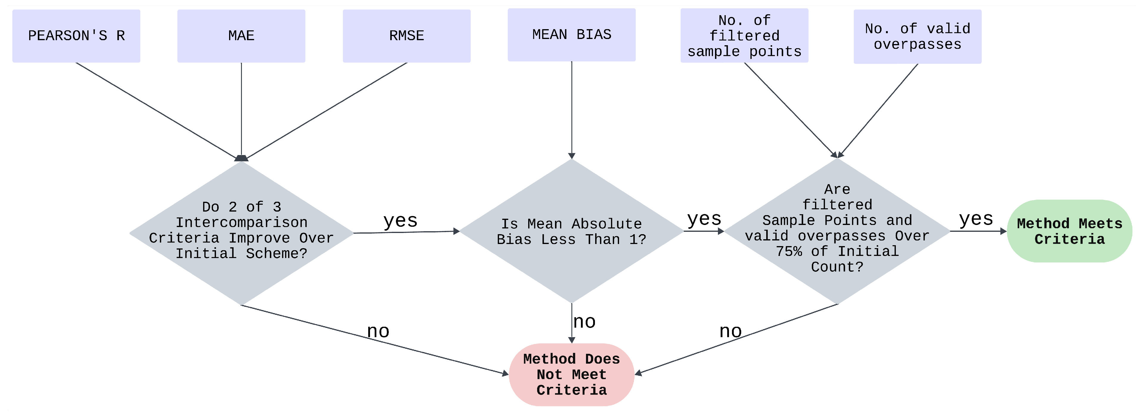
The above parameters were chosen based on existing research, which has proven their validity for thresholding and filtering. A change in the values carried out for control did not show any significant improvement. The consistency of each scheme was assessed based on the flowchart delineated in Figure 5, which outlines the sequential steps involved in the process. These steps include the determination of whether the intercomparison criteria were improved (by checking if the absolute bias was below 1), and ensuring that both the filtered sample points and valid overpasses exceed 75% of the initial count. The flowchart in Figure 5 can be used independently of the methods and is flexible, allowing other researchers to adapt it to their goals. Section 5 discusses in detail how the results can reveal which thresholds and/or filtering methods improve the agreement between the two datasets. The intercomparison criteria that were considered are the following:

• the Pearson’s correlation coefficient (R):

  $$R={\displaystyle \frac{{\sum }_{i=1}^n(Z_{\mathrm{ground},i}-\overline{Z_{\mathrm{ground}}})(Z_{\mathrm{GPM},i}-\overline{Z_{\mathrm{GPM}}})}{\sqrt{{\sum }_{i=1}^n{(Z_{\mathrm{ground},i}-\overline{Z_{\mathrm{ground}}})}^2}\sqrt{{\sum }_{i=1}^n{(Z_{\mathrm{GPM},i}-\overline{Z_{\mathrm{GPM}}})}^2}}},$$

  (3)
• the Mean Absolute Error (MAE):

  $$MAE={\displaystyle \frac{1}{n}}\sum _{i=1}^n\left|Z_{\mathrm{GPM},i}-Z_{\mathrm{ground},i}\right|,$$

  (4)
• the Root Mean Squared Error (RMSE):

  $$\mathrm{RMSE}=\sqrt{{\displaystyle \frac{1}{n}}\sum _{i=1}^n{\left(Z_{\mathrm{GPM},i}-Z_{\mathrm{ground},i}\right)}^2},$$

  (5)
• the Mean Bias:

  $$\mathrm{Mean}\mathrm{Bias}={\displaystyle \frac{1}{n}}\sum _{i=1}^n\left(Z_{\mathrm{GPM},i}-Z_{\mathrm{ground},i}\right),$$

  (6)

where, i denotes the sample point and n denotes the total number of sample points; R, RMSE and MAE were chosen to capture trends and account for the magnitude and the distribution of errors, while Mean Bias was considered to evaluate whether there is a significant over- or underestimation. Although Pearson’s R assumes normality and linearity, it remains widely used in radar reflectivity intercomparisons due to its interpretability. In our case, the reflectivity data exhibit a largely monotonic and near-linear relationship (Figure 6 and Figure 7), supporting its use. Additionally, our analysis emphasizes relative improvements in R across different selection criteria rather than its absolute value, making it a practical criterion, even when ideal assumptions are not strictly met. The amount of filtered sample points and valid overpasses were set as criteria in order to make sure that there is a representative data coverage, even under the more stringent conditions.

The schemes that met the criteria described above, were subsequently integrated into one comprehensive scheme. Applying the filtering criteria and the thresholds of this integrated scheme, we repeated the volume matching and considered the ultimate matched-up samples in identifying stable calibration periods.

Because no maintenance log was available, an attempt to identify any hardware changes was made by examining certain parameters typically adjusted during maintenance and noting the periods when these parameters remained constant. The parameter analysis was conducted on a hydrological year basis, taking into account the radar shutdown during the dry season. In this study, the hydrological year refers to a 12-month period starting on 1 October and ending on 30 September of the following year. Stable calibration periods were identified by comparing the offset distribution derived from the comprehensive volume matching scheme with the parameters’ stability over time. Then, for each stable calibration period identified, a final offset was chosen.

4. Results

This study investigated various thresholds and filtering methods to improve the consistency of the volume-matched samples between the two ground radars of the Cyprus radar network, on the one hand, and the GPM Ku, on the other hand. Through the analysis of 10 independent schemes, we identified an optimal method for each radar. The selected schemes were then applied to identify stable calibration periods per radar, combining the chosen volume matching scheme with the temporal stability of certain radar parameters. For each stable period, a final offset was determined.

The results are organized into two parts. Section 4.1 discusses the volume matching thresholds and data filtering schemes, while Section 4.2 focuses on the identification of stable calibration periods and the derivation of the final offsets.

4.1. Volume-Matching Thresholds and Data Filtering

This section evaluates the volume matching thresholds and filtering schemes.

Table 3. Summary of Pearson’s correlation coefficient (R), Mean Absolute Error (MAE), Root Mean Squared Error (RMSE) and Mean Bias between the GPM Ku and the LCA radar volume-matched samples for the initial (A) and the selected (C2, C3 and G) schemes. The table also includes the final number of sample points after applying filters and thresholds, and the number of valid satellite overpasses considered.

Scheme	Pearson’s R [−]	MAE [dBZ]	RMSE [dBZ]	Mean Bias [dBZ]	Filtered Sample Points	Valid Overpasses
A	0.676	4.094	5.506	0.099	5918	29
C2	0.611	3.793	5.173	0.611	5091	30
C3	0.661	3.946	5.295	0.163	5449	30
G	0.681	4.037	5.406	0.034	5957	30

and

Table 4. Summary of Pearson’s correlation coefficient (R), Mean Absolute Error (MAE), Root Mean Squared Error (RMSE) and Mean Bias between the GPM Ku and the PFO radar volume-matched samples for the initial (A) and the selected (C2, C3 and D) schemes. The table also includes the final number of sample points after applying filters and thresholds, and the number of valid satellite overpasses considered.

Scheme	Pearson’s R [−]	MAE [dBZ]	RMSE [dBZ]	Mean Bias [dBZ]	Filtered Sample Points	Valid Overpasses
A	0.402	4.773	9.007	−0.170	3824	34
C2	0.332	4.460	8.726	0.026	3529	34
C3	0.360	4.455	8.863	0.069	3574	34
D	0.450	4.584	8.965	−0.387	3354	30

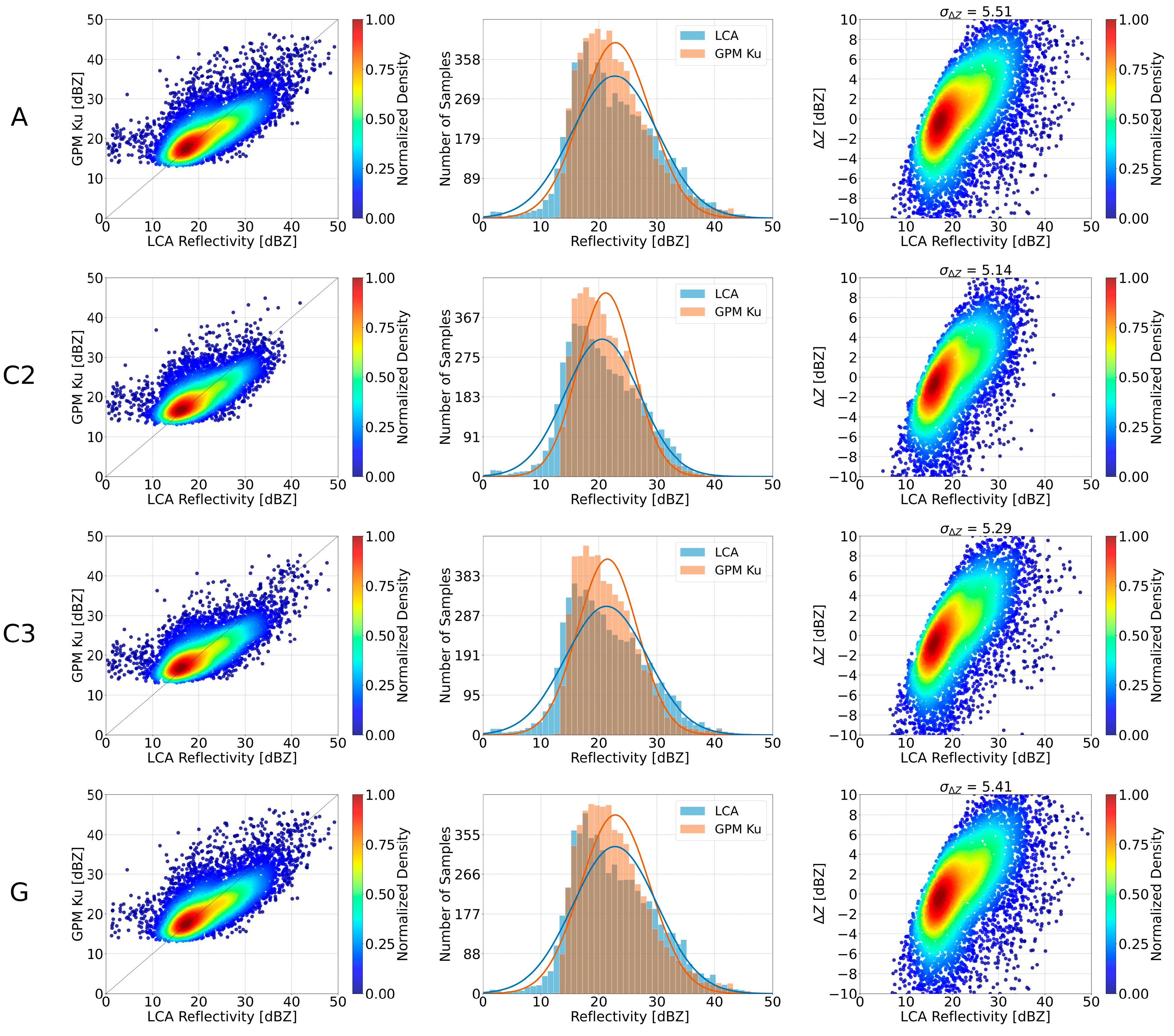
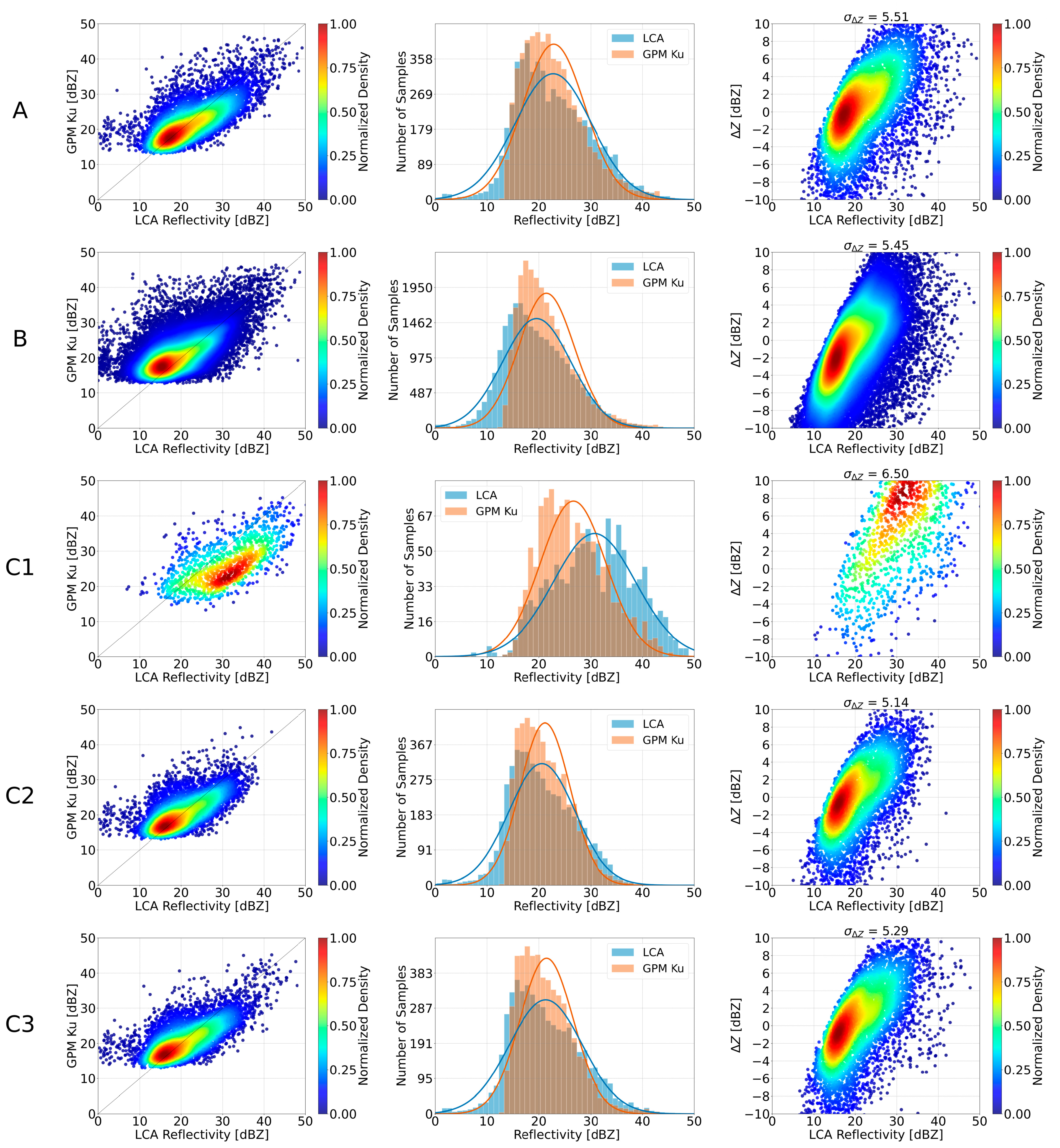
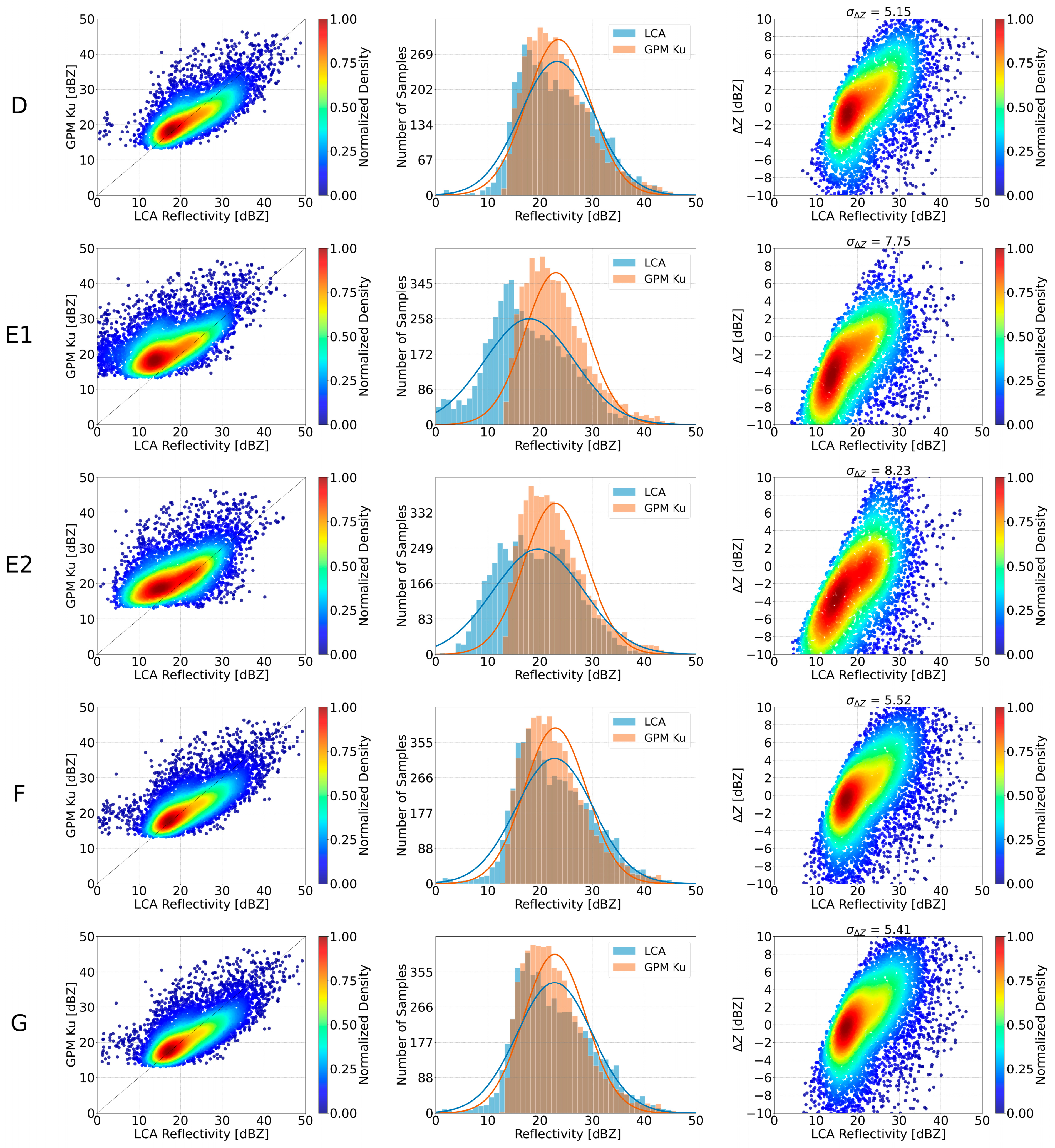
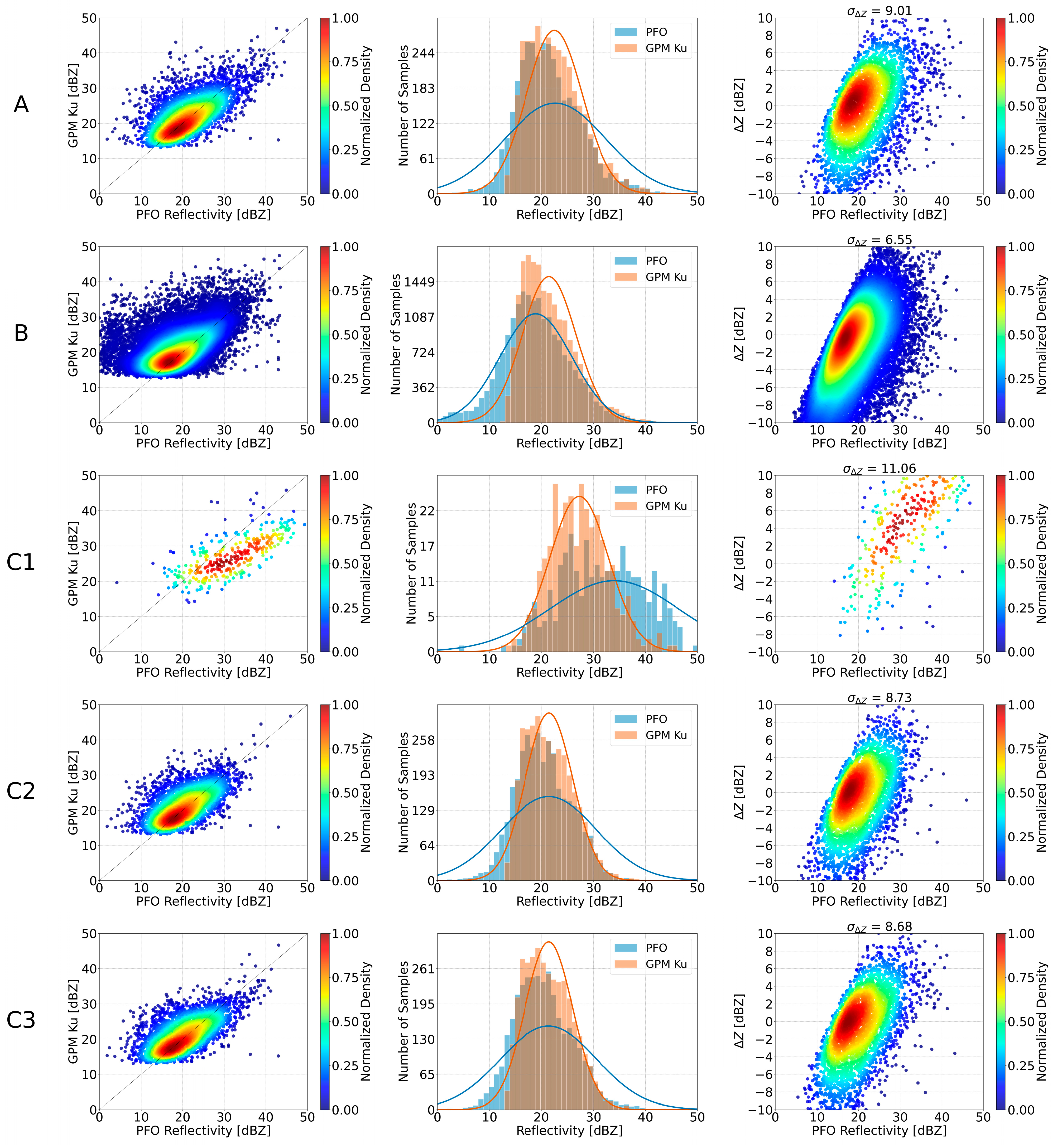
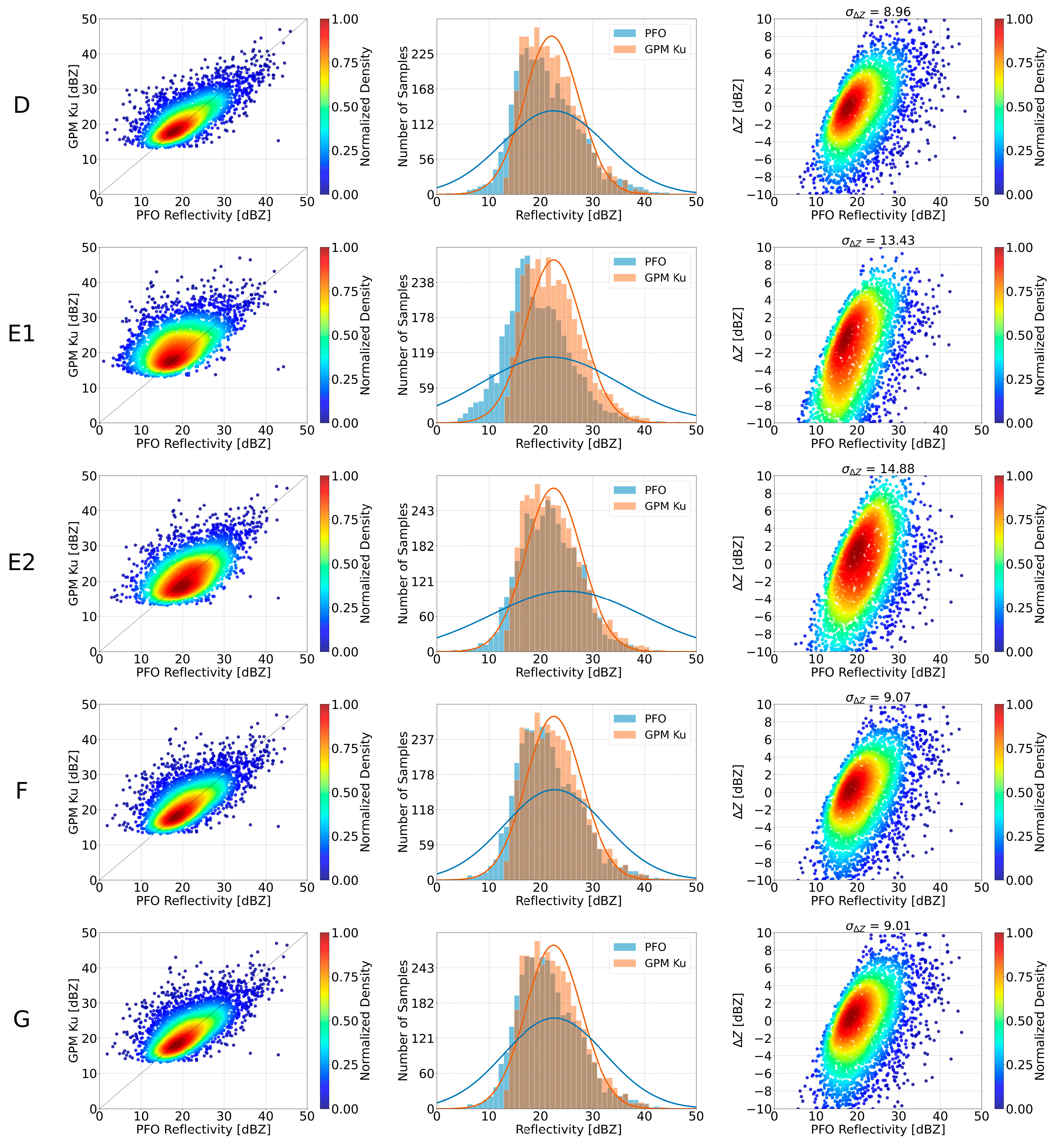
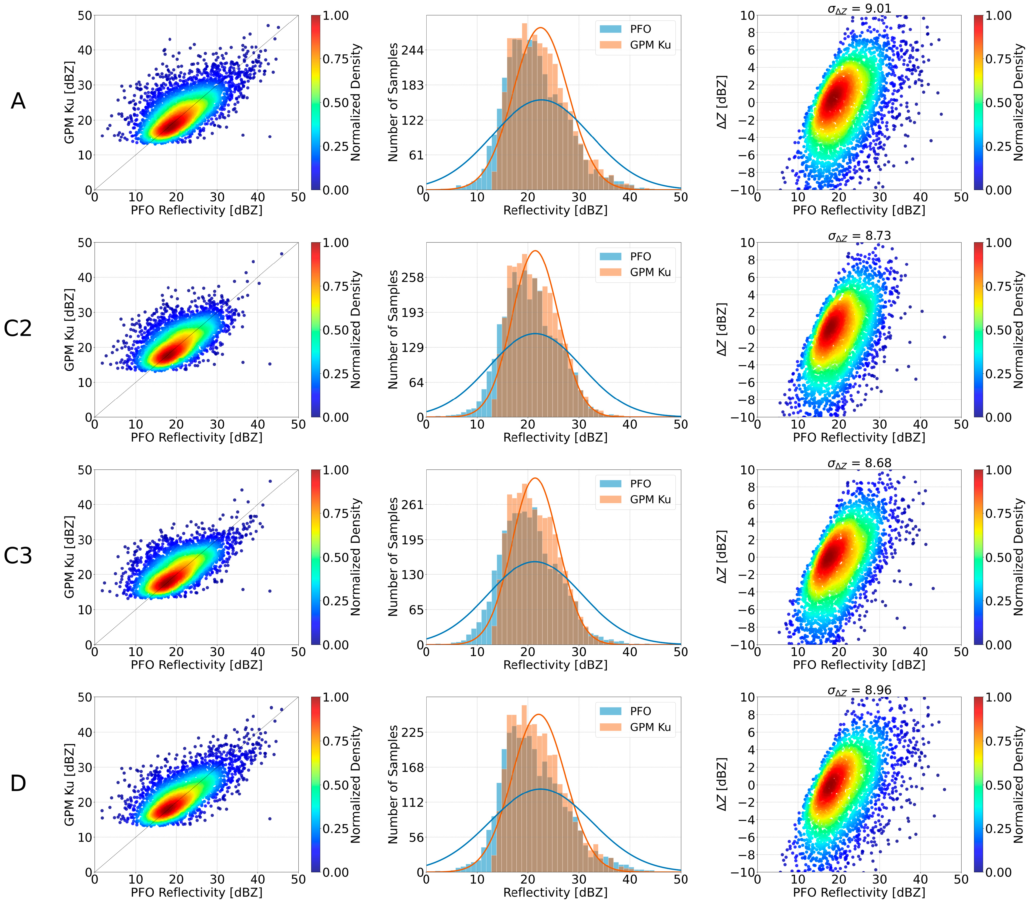
summarize the intercomparison criteria between the GPM Ku and the LCA and PFO radars volume-matched samples, respectively. The Tables also present the final number of the sample points after applying filtering and thresholds, as well as the number of valid satellite overpasses considered, and provide only the results of the schemes that met the criteria for the LCA and PFO radars. Figure 6 and Figure 7 provide the results of the initial scheme (A), together with the results of the schemes that met the criteria for LCA and PFO, respectively. The left column shows the scatter density plots of volume-matched reflectivity between GPM Ku and the ground radars, where the diagonal line represents perfect agreement between the two datasets. The middle column provides the histograms together with the probability density distribution of the volume-matched samples. In these plots, the GPM Ku samples are shown in orange, and the ground radar samples in blue. The Gaussian curves overlaid on the histograms provide a visual reference for the overall shape and spread of the reflectivity distributions. The aim is to highlight similarities or differences in the central tendency and dispersion between the ground radar and GPM Ku samples, not to suggest that the data distributions are Gaussian. The right column presents the scatter density plots of the reflectivity difference ($\Delta Z$) compared to the the ground radar volume-matched reflectivity. Each row is numbered, with the row numbers corresponding to the selected schemes. Each row is marked with the corresponding scheme. The results of all schemes are presented in Appendix A.

With regard to the LCA radar, schemes C2, C3 and G met the criteria we defined. The results of scheme A suggested that the volume-matched reflectivities from the two radars (LCA and GPM Ku) were generally in agreement, particularly in the range between 15 and 20 dBZ. However, as the reflectivity values increased, the scatter points shifted below the diagonal line, indicating reflectivity overestimation for the LCA radar in the range between 20 and 30 dBZ. Schemes C2 and C3 resulted in similar distributions, with the sample points exhibiting greater concentration around the distribution’s density peak. The histogram plots revealed important insights into the distribution of the volume-matched reflectivity samples. For schemes A, C2 and C3, both the LCA and the GPM Ku volume-matched reflectivities fell within a similar range, with negligible differences. The normalized density plots between the reflectivity difference ($\Delta Z$) and the ground radar volume-matched reflectivity demonstrated the consistency of the volume matching with regard to the magnitude of the LCA radar reflectivity. Schemes A, C2 and C3 resulted in differences predominantly between −4 and 4 dBZ for the LCA reflectivities in the range between 10 and 20 dBZ. As the LCA reflectivity increased, the differences tended to increase as well. Scheme G yielded almost identical results to those of Scheme A. Across the selected schemes, the differences were concentrated around zero, but showed a growing spread for reflectivities higher than 25 dBZ. A subtle shift was observed in the distribution of scheme A, where the highest density area is slightly displaced, but this is no longer observed in schemes C2 and C3. Additionally, schemes C2 and C3 decreased the standard deviation of the reflectivity differences.

The above-described results are reflected in the intercomparison criteria as well. Pearson’s R did not improve with schemes C2 and C3, but maintained a strong linear agreement between the GPM Ku and the ground radar volume-matched samples. Schemes C2, C3 and G yielded lower MAE and a slightly improved RMSE compared to scheme A. Both scheme A, C3 and G maintained a near-zero bias. Schemes C2, C3 and G retained a satisfactory number of filtered sample points and valid overpasses.

With regard to the PFO radar, schemes C2, C3 and D met the established criteria. The density plots confirmed the strong agreement between the PFO radar and the GPM Ku volume-matched reflectivities, with all selected schemes showing a similar distribution. The points corresponding to schemes C2 and C3 were more heavily gathered along the 1:1 line compared to the behavior of rest schemes. The histogram plots exhibited similar results for all selected schemes, though schemes C2 and C3 resulted in slightly more symmetric histograms, particularly for reflectivities higher than 25 dBZ. Similar to the LCA radar, reflectivity differences for the PFO radar were mostly concentrated within −4 and 4 dBZ for reflectivities below 20 dBZ, but demonstrated a broader spread for reflectivities above 25 dBZ. Schemes C2 and C3 yielded a lower standard deviation of the reflectivity differences and a better consistency in $\Delta Z$ clustering.

In terms of intercomparison, schemes C2 and C3 did not show any improvements in Pearson’s R compared to scheme A, while scheme D achieved the highest Pearson’s R (0.45). However, schemes C2, C3 and D improved MAE and RMSE relative to scheme A. Across all selected schemes, the systematic bias remained near zero. As observed for the LCA radar, the selected schemes for the PFO radar maintained a reliable number of filtered sample points and valid overpasses.

4.2. Stable Calibration Periods and Final Offsets

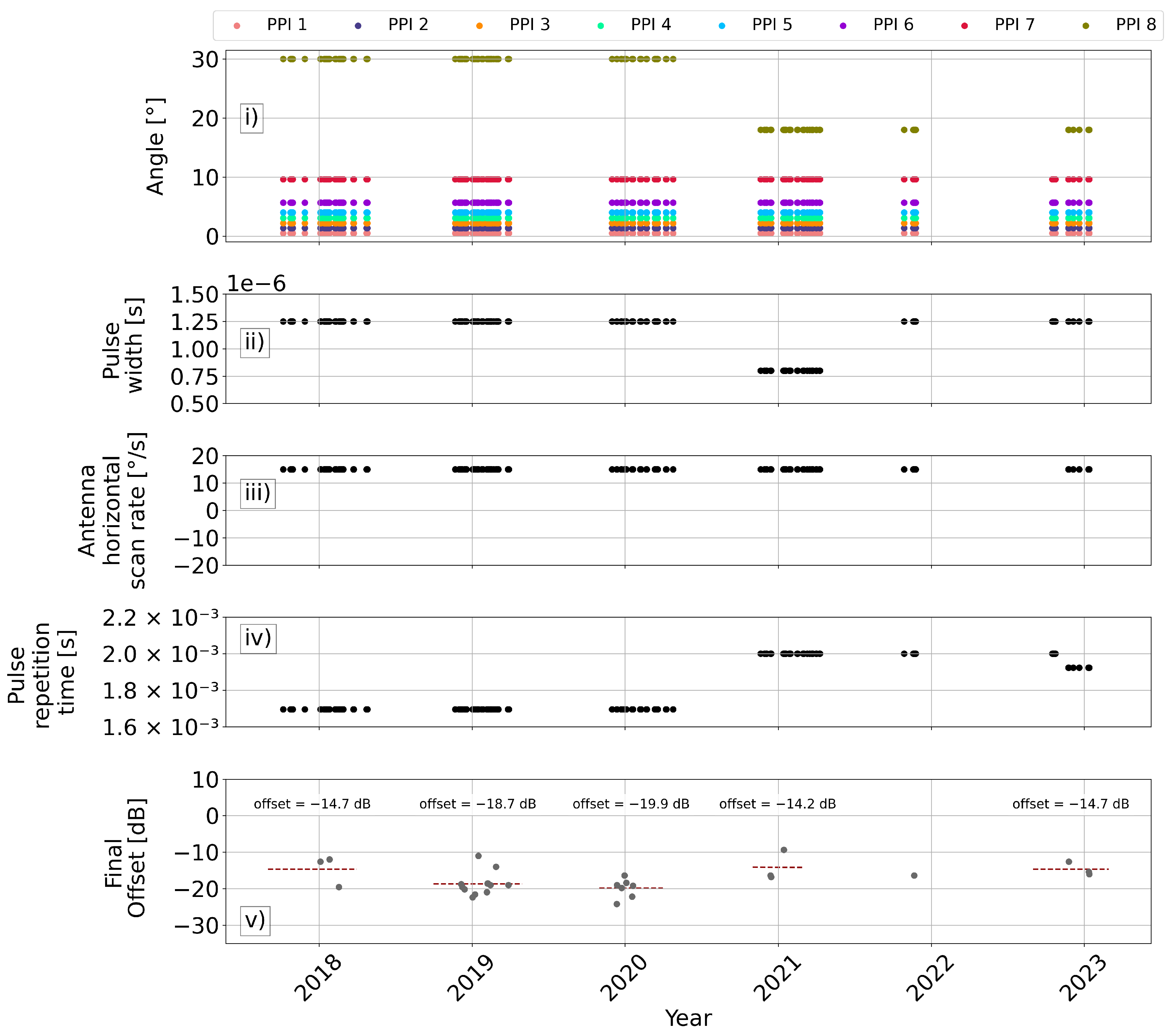
For the identification of the stable calibration periods, we assessed the stability of the eight fixed elevation angles, the pulse width [s], the antenna horizontal scan rate [°/s], and the pulse repetition time s. As shown in Figure 8i, the fixed elevation angles enabled the identification of two distinct periods during which their behavior differed: hydrological years 2017–2020 and 2020–2023). The pulse width showed a clustering into three different periods: hydrological years 2017–2020, 2020–2021, and 2021–2023 (Figure 8ii). The antenna horizontal scan rate remained constant during the entire study period (Figure 8iii), while the pulse repetition time appeared to be clustered in two periods, following the configuration of the fixed angles. A minor drop in the pulse repetition time from $2.0\times {10}^{-3}$ s to $1.7\times {10}^{-3}$ s was observed after the first months of hydrological year 2022–2023 (Figure 8iv).

Following the above insights and based on the number of valid satellite overpasses per year, we distinguished two stable calibration periods for the LCA radar: hydrological years 2018–2019, and 2019–2020. Hydrological years 2017–2018, 2020–2021 and 2021–2022 could not be considered stable periods, due to the limited number of valid satellite overpasses. The remaining period (2022–2023) was not considered due to the instability of the pulse repetition time. The final offset of each stable calibration period was determined by calculating the average of the calibration offsets estimated within that timeframe. As demonstrated in Figure 8v, the final offset for 2018–2019 was estimated at −18.7 dB and for 2019–2020 at −19.9 dB.

The fixed elevation angles for the PFO radar exhibited the same pattern as those of the LCA radar, indicating two stable periods: hydrological years 2017–2020 and 2020–2023 (Figure 9i). The pulse width suggested stability in the hydrological years 2017–2018, 2019–2020, 2020–2021 and 2022–2023 (Figure 9ii). The antenna horizontal scan rate remained constant throughout the entire study period, except for a drop in a few records during hydrological year 2019–2020 (Figure 9iii). The pulse repetition time indicated three stable periods: hydrological years 2017–2020, 2020–2021 and 2022–2023, while its behavior during 2021–2022 presented some fluctuations (Figure 9iv).

Based on the above observations, as well as the number of valid satellite overpasses per year, we distinguished two stable calibration periods for the PFO radar: hydrological years 2019–2020 and 2022–2023. Hydrological years 2017–2018 and 2020–2021 were not taken into account due to the limited number of valid satellite overpasses, while hydrological years 2018–2019 and 2021–2022 could not be considered as stable periods due to the observed fluctuations in the examined parameters. The final offsets for the two stable calibration periods were calculated at −19.8 dB and −9.1 dB for the periods between 2019–2020 and 2022–2023, respectively (Figure 9v).

5. Discussion

The findings of this study highlight the importance of careful selection of methodology when calibrating ground radars against satellite data by using the volume-matching method. Including only reflectivities above the melting layer (Scheme C2) and masking out the melting layer with a buffer distance of 250 m (Scheme C3) was found to yield more consistent calibration results for both LCA and PFO radars. Increasing the minimum fraction from $f_{min}=0.7$ to $f_{min}=0.9$ (Scheme G) performed well for LCA radar, while masking the reflectivities affected by the cumulative beam blockage (Scheme D) was proven effective for the PFO radar.

The volume-matched samples of the PFO radar showed an overall lower correlation with the GPM Ku samples. This might be associated to the PFO radar’s location, which is hillier and more prone to heavier rain events. Heavier rain leads to increased attenuation, which might explain the observed lower correlation.

With regard to the results of the remaining schemes (see Appendix A), there are several outcomes worth discussing. In particular, when considering only reflectivities from stratiform precipitation (Scheme B), we observed that more volume-matched samples could be filtered, with the samples demonstrating a major spread around the core of the density plots. In contrast, Scheme C1, which included only the reflectivities below the melting layer, led to the exclusion of a notable number of volume-matched samples and resulted in a considerable reflectivity overestimation for both ground radars. As part of the examined schemes, reflectivities were filtered to include only values between 19 dBZ and 25 dBZ (Scheme E1), and between 24 dBZ and 36 dBZ (Scheme E2), as applied by Pejcic et al. [8] and Warren et al. [7], respectively. In the present study, both schemes E1 and E2 resulted in overestimated reflectivities by the GPM Ku, as well as higher bias for both ground radars.

In addition to examining the impact of the singled-out schemes, it is also essential to consider the role of temporal factors, such as the variability in meteorological conditions between different hydrological years. A notable observation is that the hydrological year 2019–2020 yielded consistent results for both ground radars. This could imply that the operational settings during this period were more appropriate for the Cyprus radar network. Yet, this implication cannot be exhaustive, as hydrological year 2019–2020 was a wet year in Cyprus. The consistency of the results for this year might be linked to the wealth of volume-matched samples that were available for calibration during this year. This finding underscores that the method presented in this work is also strongly dependent on the meteorological characteristics specific to each case. On the one hand, the method has the potential to reveal more insights when applied for records from rainier regions. On the other hand, it might be inadequate in calibrating of ground radars in drier regions. In such regions, the absolute calibration method [43] might be more suitable.

The final offset for both the LCA and the PFO radars before the radar range change (hydrological years 2018–2019 and 2019–2020) was found obtaining values around −20 dB, indicating critical miscalibration during that period. Offsets of this magnitude render ground radar data unsuitable for precise quantitative purposes, such as the assessment of rain intensity and the classification of hydrometeors. Records affected by such offsets can only provide a qualitative indication of the severity of a rain event, by evaluating the range within which the measured reflectivity values vary.

The analysis of the stability of the radar parameters revealed valuable insights for the identification of stable calibration periods. While this method is not commonly used for identifying stable calibration periods, it proved effective in our case. One could characterize our selection of stable calibration periods as conservative, because it excluded periods with a sufficient number of valid overpasses, solely due to instability in a radar parameter. Even so, this scheme helped us ensure that the chosen stable periods are reliable and accurate, providing more robust results.

Our method builds on the volume-matching method, which has already been successfully applied in different climatic conditions and primarily for C-band and S-band meteorological radars. The proposed methodology enhances the applicability of the volume-matching method, as it dynamically fine-tunes the method by selecting the optimal thresholds and filters directly based on the data. This data-driven enhancement adapts the method to the specific climatic, regional and radar characteristics, and thereby improves the calibration accuracy and robustness.

6. Conclusions

The absolute calibration of ground radar data using GPM Ku was examined by various authors, who set different constraints and filters in their respective procedures. This study applied constraints and filters found in the literature following a singled-out scheme in order to identify those yielding consistent volume-matched samples for the LCA and PFO radars of the Cyprus radar network. The evaluation of the schemes was done based on the Pearson’s R, the RMSE, the MAE and the Mean Bias, as well as the number of the filtered sample points and the valid overpasses.

The results revealed that masking the reflectivities below, inside the melting layer and in a buffer distance of 250 m yielded more consistent calibration for both the LCA and the PFO radars. PFO radar calibration was also improved when we masked out the records that were affected by cumulative beam blockage (Scheme D), while LCA radar calibration was improved when we applied the stricter minimum fraction of 0.9. The selected schemes were combined to finalize the calibration of each ground radar.

Once the optimal calibration methods were selected, we compared the stability of the resulting offsets to the stability of certain radar parameters that are typically set during maintenance and were not expected to vary in time. This procedure helped us identify stable calibration periods, as we had no auxiliary information on this matter. For each stable calibration period we estimated the final offset by averaging the calibration offsets during that period. We yielded two stable calibration periods for each radar. For the LCA radar those were the hydrological years 2018–2019 and 2019–2020 with final offsets −18.7 dB and −19.9 dB, respectively. For the PFO radar hydrological years 2019–2020 and 2022–2023 were selected as stable calibration periods and their final offsets were calculated at −19.8 dB and −9.1 dB, respectively.

Overall, this study highlights the need for adaptive, region- and radar-specific calibration methods, especially in complex meteorological environments, such as those encountered in the Mediterranean environment. Our work represents a significant advancement in radar calibration techniques, by introducing a procedure that relies solely on GPM Ku data, without the need for supplementary data. This study differs from previous research, as it compares and evaluates various methods from the existing literature, such as separately filtering out the reflectivities measured above and below the melting layer, and determines the optimal strategy based on the results obtained. Notably, we observed that some methods followed in other studies were not applicable in our context, highlighting the importance of adapting the volume-matching method to the characteristics of the examined case study.

The findings of this study will be communicated to the Cyprus Department of Meteorology and are expected to contribute in enhancing the radar data analysis process, as well as in the more effective maintenance of the radars. The developed framework presents an operational, time-resolved calibration method for the Cyprus weather radars that is able to track changes in radar calibration. The absolute calibration method is needed to deliver vital high resolution precipitation analysis to Cyprus, where no other time- and area-comprehensive radar coverage is available. Based on the outcomes of this study, it is recommended that the maintenance carried out before the radars become operational for the hydrological year 2019–2020 was the most suitable practice.

Future work includes the application of the final offset to the ground radars. Using the calibrated radar data from the entire Cyprus radar network, we plan to extend our analysis to include the estimation of the quantitative precipitation. Additionally, we anticipate complementing the radar calibration procedure with measurements form the disdrometer that was recently installed at the Cyprus Atmospheric Remote Sensing Observatory (CARO), as soon as it records a sufficient number of measurements. These efforts will contribute to the enhancement of radar-based meteorological applications in Cyprus, supporting both research and operational applications.

References

1. Das, S.K.; Krishna, U.V.M.; Kolte, Y.K.; Deshpande, S.M.; Pandithurai, G. Assessment of Ground-Based X-Band Radar Reflectivity: Attenuation Correction and its Comparison With Space-Borne Radars Over the Western Ghats, India. Earth Space Sci. 2020, 7, e2019EA000861. [Google Scholar] [CrossRef]
2. Pejcic, V.; Simmer, C.; Trömel, S. Polarimetric radar-based methods for evaluation of hydrometeor mixtures in numerical weather prediction models. In Proceedings of the 2021 21st International Radar Symposium (IRS), Berlin, Germany, 21–22 June 2021; pp. 1–10. [Google Scholar] [CrossRef]
3. Kou, L.; Mao, Y.; Wang, Z.; Lin, Z.; Chen, Y.; Gao, H.; Chu, Z.; Chen, A. Comparisons of three-dimensional reflectivity and precipitation rate from GPM dual-frequency precipitation radar and ground dual-polarization radar. Atmos. Res. 2023, 282, 106521. [Google Scholar] [CrossRef]
4. Ryzhkov, A.; Zhang, P.; Bukovčić, P.; Zhang, J.; Cocks, S. Polarimetric Radar Quantitative Precipitation Estimation. Remote Sens. 2022, 14, 1695. [Google Scholar] [CrossRef]
5. Maki, M.; Kim, Y.; Kobori, T.; Hirano, K.; Lee, D.I.; Iguchi, M. Analyses of three-dimensional weather radar data from volcanic eruption clouds. J. Volcanol. Geotherm. Res. 2021, 412, 107178. [Google Scholar] [CrossRef]
6. Frech, M.; Hagen, M.; Mammen, T. Monitoring the Absolute Calibration of a Polarimetric Weather Radar. J. Atmos. Ocean. Technol. 2017, 34, 599–615. [Google Scholar] [CrossRef]
7. Warren, R.A.; Protat, A.; Siems, S.T.; Ramsay, H.A.; Louf, V.; Manton, M.J.; Kane, T.A. Calibrating Ground-Based Radars against TRMM and GPM. J. Atmos. Ocean. Technol. 2018, 35, 323–346. [Google Scholar] [CrossRef]
8. Pejcic, V.; Soderholm, J.; Mühlbauer, K.; Louf, V.; Trömel, S. Five years calibrated observations from the University of Bonn X-band weather radar (BoXPol). Sci. Data 2022, 9, 551. [Google Scholar] [CrossRef]
9. Zhong, L.; Yang, R.; Chen, L.; Wen, Y.; Li, R.; Tang, G.; Hong, Y. Combined Space and Ground Radars for Improving Quantitative Precipitation Estimations in the Eastern Downstream Region of the Tibetan Plateau. Part I: Variability in the Vertical Structure of Precipitation in ChuanYu Analyzed from Long-Term Spaceborne Observations by TRMM PR. J. Appl. Meteorol. Climatol. 2017, 56, 2259–2274. [Google Scholar] [CrossRef]
10. Han, J.; Chu, Z.; Wang, Z.; Xu, D.; Li, N.; Kou, L.; Xu, F.; Zhu, Y. The establishment of optimal ground-based radar datasets by comparison and correlation analyses with space-borne radar data. Meteorol. Appl. 2018, 25, 161–170. [Google Scholar] [CrossRef]
11. Crisologo, I.; Warren, R.A.; Mühlbauer, K.; Heistermann, M. Enhancing the consistency of spaceborne and ground-based radar comparisons by using beam blockage fraction as a quality filter. Atmos. Meas. Tech. 2018, 11, 5223–5236. [Google Scholar] [CrossRef]
12. Protat, A.; Louf, V.; Soderholm, J.; Brook, J.; Ponsonby, W. Three-way calibration checks using ground-based, ship-based, and spaceborne radars. Atmos. Meas. Tech. 2022, 15, 915–926. [Google Scholar] [CrossRef]
13. Gabella, M.; Notarpietro, R. Ground clutter characterization and elimination in mountainous terrain. In Proceedings of the ERAD, Delft, The Netherlands, 18–22 November 2002; pp. 305–311. [Google Scholar]
14. Doviak, R.J.; Zrnić, D.S. Reflection and scatter formula for anisotropically turbulent air. Radio Sci. 1984, 19, 325–336. [Google Scholar] [CrossRef]
15. Wilson, J.W.; Brandes, E.A. Radar Measurement of Rainfall—A Summary. Bull. Am. Meteorol. Soc. 1979, 60, 1048–1058. [Google Scholar] [CrossRef]
16. Germann, U.; Joss, J. Operational Measurement of Precipitation in Mountainous Terrain. In Weather Radar, Principles and Advanced Applications; Springer: Berlin/Heidelberg, Germany, 2004; pp. 52–77. [Google Scholar] [CrossRef]
17. Gabella, M.; Morin, E.; Notarpietro, R.; Michaelides, S. Winter precipitation fields in the Southeastern Mediterranean area as seen by the Ku-band spaceborne weather radar and two C-band ground-based radars. Atmos. Res. 2013, 119, 120–130. [Google Scholar] [CrossRef]
18. Crisologo, I.; Heistermann, M. Using ground radar overlaps to verify the retrieval of calibration bias estimates from spaceborne platforms. Atmos. Meas. Tech. 2020, 13, 645–659. [Google Scholar] [CrossRef]
19. Villarini, G.; Krajewski, W.F. Review of the Different Sources of Uncertainty in Single Polarization Radar-Based Estimates of Rainfall. Surv. Geophys. 2010, 31, 107–129. [Google Scholar] [CrossRef]
20. Houze Jr, R.A.; Brodzik, S.; Schumacher, C.; Yuter, S.E.; Williams, C.R. Uncertainties in Oceanic Radar Rain Maps at Kwajalein and Implications for Satellite Validation. J. Appl. Meteorol. 2004, 43, 1114–1132. [Google Scholar] [CrossRef]
21. Wang, J.; Wolff, D.B. Comparisons of Reflectivities from the TRMM Precipitation Radar and Ground-Based Radars. J. Atmos. Ocean. Technol. 2009, 26, 857–875. [Google Scholar] [CrossRef]
22. Seo, B.C.; Krajewski, W.F.; Smith, J.A. Four-dimensional reflectivity data comparison between two ground-based radars: Methodology and statistical analysis. Hydrol. Sci. J. 2014, 59, 1320–1334. [Google Scholar] [CrossRef]
23. Joss, J.; Gabella, M.; Michaelides, S.C.; Perona, G. Variation of weather radar sensitivity at ground level and from space: Case studies and possible causes. Meteorol. Z. 2006, 15, 485–496. [Google Scholar] [CrossRef]
24. Kubota, T.; Yoshida, N.; Urita, S.; Iguchi, T.; Seto, S.; Meneghini, R.; Awaka, J.; Hanado, H.; Kida, S.; Oki, R. Evaluation of Precipitation Estimates by at-Launch Codes of GPM/DPR Algorithms Using Synthetic Data from TRMM/PR Observations. IEEE J. Sel. Top. Appl. Earth Obs. Remote Sens. 2014, 7, 3931–3944. [Google Scholar] [CrossRef]
25. Toyoshima, K.; Masunaga, H.; Furuzawa, F.A. Early Evaluation of Ku- and Ka-Band Sensitivities for the Global Precipitation Measurement (GPM) Dual-Frequency Precipitation Radar (DPR). SOLA 2015, 11, 14–17. [Google Scholar] [CrossRef]
26. Anagnostou, E.N.; Morales, C.A.; Dinku, T. The use of TRMM precipitation radar observations in determining ground radar calibration biases. J. Atmos. Ocean. Technol. 2001, 18, 616–628. [Google Scholar] [CrossRef]
27. Liao, L.; Meneghini, R.; Iguchi, T. Comparisons of Rain Rate and Reflectivity Factor Derived from the TRMM Precipitation Radar and the WSR-88D over the Melbourne, Florida site. J. Atmos. Ocean. Technol. 2001, 18, 1959–1974. [Google Scholar] [CrossRef]
28. Islam, T.; Rico-Ramirez, M.A.; Han, D.; Srivastava, P.K.; Ishak, A.M. Performance evaluation of the TRMM precipitation estimation using ground-based radars from the GPM validation network. J. Atmos. -Sol.-Terr. Phys. 2012, 77, 194–208. [Google Scholar] [CrossRef]
29. Gabella, M.; Joss, J.; Perona, G.; Michaelides, S. Range adjustment for ground-based radar, derived with the spaceborne TRMM precipitation radar. IEEE Trans. Geosci. Remote Sens. 2006, 44, 126–133. [Google Scholar] [CrossRef]
30. Gabella, M.; Morin, E.; Notarpietro, R. Using TRMM spaceborne radar as a reference for compensating ground-based radar range degradation: Methodology verification based on rain gauges in Israel. J. Geophys. Res. 2011, 116, D02114. [Google Scholar] [CrossRef]
31. Bringi, V.N.; Huang, G.J.; Munchak, S.J.; Kummerow, C.D.; Marks, D.A.; Wolff, D.B. Comparison of Drop Size Distribution Parameter (D0) and Rain Rate from S-Band Dual-Polarized Ground Radar, TRMM Precipitation Radar (PR), and Combined PR–TMI: Two Events from Kwajalein Atoll. J. Atmos. Ocean. Technol. 2012, 29, 1603–1616. [Google Scholar] [CrossRef]
32. Park, S.; Jung, S.H.; Lee, G. Cross Validation of TRMM PR Reflectivity Profiles Using 3D Reflectivity Composite from the Ground-Based Radar Network over the Korean Peninsula. J. Hydrometeorol. 2015, 16, 668–687. [Google Scholar] [CrossRef]
33. Zhang, S.; Zhu, Y.; Wang, Z.; Wang, Y. Consistency analysis and correction of ground-based radar observations using space-borne radar. J. Atmos. -Sol.-Terr. Phys. 2018, 169, 114–121. [Google Scholar] [CrossRef]
34. Bolen, S.M.; Chandrasekar, V. Methodology for Aligning and Comparing Spaceborne Radar and Ground-Based Radar Observations. J. Atmos. Ocean. Technol. 2003, 20, 647–659. [Google Scholar] [CrossRef]
35. Schwaller, M.R.; Morris, K.R. A ground validation network for the global precipitation measurement mission. J. Atmos. Ocean. Technol. 2011, 28, 301–319. [Google Scholar] [CrossRef]
36. Kim, J.H.; Ou, M.L.; Park, J.D.; Morris, K.R.; Schwaller, M.R.; Wolff, D.B. Global Precipitation Measurement (GPM) Ground Validation (GV) Prototype in the Korean Peninsula. J. Atmos. Ocean. Technol. 2014, 31, 1902–1921. [Google Scholar] [CrossRef]
37. Chen, H.; Chandrasekar, V. Validation of NASA’s Global Precipitation Measurement mission with a high-resolution ground radar network. In Proceedings of the 2016 URSI Asia-Pacific Radio Science Conference (URSI AP-RASC), Seoul, Republic of Korea, 21–25 August 2016; pp. 836–839. [Google Scholar] [CrossRef]
38. Bech, J.; Codina, B.; Lorente, J.; Bebbington, D. The Sensitivity of Single Polarization Weather Radar Beam Blockage Correction to Variability in the Vertical Refractivity Gradient. J. Atmos. Ocean. Technol. 2003, 20, 845–855. [Google Scholar] [CrossRef]
39. Biswas, S.K.; Chandrasekar, V. Cross-Validation of Observations between the GPM Dual-Frequency Precipitation Radar and Ground Based Dual-Polarization Radars. Remote Sens. 2018, 10, 1773. [Google Scholar] [CrossRef]
40. Meneghini, R.; Kim, H.; Liao, L.; Kwiatkowski, J.; Iguchi, T. Path attenuation estimates for the GPM dual-frequency precipitation radar (DPR). J. Meteorol. Soc. Jpn. 2021, 99, 181–200. [Google Scholar] [CrossRef]
41. Huang, H.; Zhao, K.; Fu, P.; Chen, H.; Chen, G.; Zhang, Y. Validation of Precipitation Measurements From the Dual-Frequency Precipitation Radar Onboard the GPM Core Observatory Using a Polarimetric Radar in South China. IEEE Trans. Geosci. Remote Sens. 2022, 60, 4104216. [Google Scholar] [CrossRef]
42. Keem, M.; Seo, B.C.; Krajewski, W.F.; Morris, K.R. Inter-comparison of reflectivity measurements between GPM DPR and NEXRAD radars. Atmos. Res. 2019, 226, 49–65. [Google Scholar] [CrossRef]
43. Wolff, D.B.; Marks, D.A.; Petersen, W.A. General Application of the Relative Calibration Adjustment (RCA) Technique for Monitoring and Correcting Radar Reflectivity Calibration. J. Atmos. Ocean. Technol. 2015, 32, 496–506. [Google Scholar] [CrossRef]
44. Louf, V.; Protat, A.; Warren, R.A.; Collis, S.M.; Wolff, D.B.; Raunyiar, S.; Jakob, C.; Petersen, W.A. An integrated approach to weather radar calibration and monitoring using ground clutter and satellite comparisons. J. Atmos. Ocean. Technol. 2019, 36, 17–39. [Google Scholar] [CrossRef]
45. Loulli, E.; Michaelides, S.; Bühl, J.; Loukas, A.; Hadjimitsis, D.G. Correction of path integrated attenuation using data from two X-band ground-based radars and GPM. Atmos. Res. 2025, 321, 108080. [Google Scholar] [CrossRef]
46. Simpson, J.; Kummerow, C.; Tao, W.K.; Adler, R.F. On the Tropical Rainfall Measuring Mission (TRMM); Springer: Berlin/Heidelberg, Germany, 1996; Volume 60, pp. 19–36. [Google Scholar]
47. Furukawa, K.; Kojima, M.; Miura, T.; Hyakusoku, Y.; Kai, H.; Ishikiri, T.; Iguchi, T.; Hanado, H.; Nakagawa, K.; Okumura, M. Satellite system test status of the Dual-Frequency Precipitation Radar on the global precipitation measurement core spacecraft. In Proceedings of the 2013 IEEE International Geoscience and Remote Sensing Symposium—IGARSS, Melbourne, VIC, Australia, 21–26 July 2013; pp. 1143–1146. [Google Scholar] [CrossRef]
48. Iguchi, T.; Seto, S.; Meneghini, R.; Yoshida, N.; Awaka, J.; Le, M.; Chandrasekar, V.; Brodzik, S.; Kubota, T.; Takahashi, N. GPM/DPR Level-2 Algorithm Theoretical Basis Document; Technical Report, NASA Technical Report; NASA Goddard Space Flight Center: Greenbelt, MD, USA, 2021. [Google Scholar]
49. Hou, A.Y.; Kakar, R.K.; Neeck, S.; Azarbarzin, A.A.; Kummerow, C.D.; Kojima, M.; Oki, R.; Nakamura, K.; Iguchi, T. The global precipitation measurement mission. Bull. Am. Meteorol. Soc. 2014, 95, 701–722. [Google Scholar] [CrossRef]
50. Olson, W.S.; Masunaga, H. The GPM Combined Radar Radiometer Algorithm Team. GPM Combined Radar-Radiometer Precipitation Algorithm Theoretical Basis Document (Version 4); NASA: Washington, DC, USA, 2016. [Google Scholar]
51. Liao, L.; Meneghini, R. Changes in the TRMM Version-5 and Version-6 Precipitation Radar Products Due to Orbit Boost. J. Meteorol. Soc. Jpn. Ser. II 2009, 87A, 93–107. [Google Scholar] [CrossRef]
52. NASA. NASA Shuttle Radar Topography Mission (SRTM) Global. Distributed by OpenTopography, 2013. Available online: https://portal.opentopography.org/datasetMetadata?otCollectionID=OT.042013.4326.1 (accessed on 25 November 2023). [CrossRef]
Figure 1. Geographical location and coverage of the two ground radars (150 km (October 2017–May 2020), 250 km (November 2020–May 2023)).
Remotesensing 17 01712 g001
Figure 2. Schematic representation of the viewing geometries of a ground radar and GPM Ku, and their volume-matched intersection.
Remotesensing 17 01712 g002
Figure 3. (a) GPM Ku overpass from 12 December 2019, 7:51 UTC, (b) LCA radar 0.5° elevation angle from 12 December 2019, 7:50 UTC, (c) Volume-matched samples GPM-LCA from 12 December 2019 at 0.5° elevation angle of GPM Ku reflectivity, (d) Volume-matched samples GPM-LCA from 12 December 2019 at 0.5° elevation angle of LCA reflectivity.
Remotesensing 17 01712 g003
Figure 4. (a) GPM Ku overpass from 12 December 2019, 7:51 UTC, (b) PFO radar 0.5° elevation angle from 12 December 2019, 7:55 UTC, (c) Volume-matched samples GPM-PFO from 12 December 2019 at 0.5° elevation angle of GPM Ku reflectivity, (d) Volume-matched samples GPM-PFO from 12 December 2019 at 0.5° elevation angle of PFO reflectivity.
Remotesensing 17 01712 g004
Figure 5. Decision-making flowchart for evaluating the consistency of the results across the examined schemes based on intercomparison metrics (Pearson’s R, MAE, RMSE), mean absolute bias, filtered sample points and valid overpasses.
Remotesensing 17 01712 g005
Figure 6. Initial (A) and selected (C2, C3 and G) schemes for the LCA radar (Left: Scatter density plots of volume-matched reflectivity between GPM Ku and LCA radar. The diagonal line represents perfect agreement between the two datasets. Middle: Histograms together with the probability density distribution of the volume-matched samples. Right: Scatter density plots of LCA - GPM Ku reflectivity difference ( Δ Z ) compared to the LCA volume-matched reflectivity).
Remotesensing 17 01712 g006
Figure 7. Initial (A) and selected (C2, C3 and D) schemes for the PFO radar (Left: Scatter density plots of volume-matched reflectivity between GPM Ku and PFO radar. The diagonal line represents perfect agreement between the two datasets. Middle: Histograms together with the probability density distribution of the volume-matched samples. Right: Scatter density plots of PFO-GPM Ku reflectivity difference ( Δ Z ) compared to the PFO volume-matched reflectivity).
Remotesensing 17 01712 g007
Figure 8. (i) Fixed angles [°], (ii) Pulse width [s], (iii) Antenna horizontal scan rate [°/s], (iv) Pulse repetition time [s], (v) final offsets [dB] per stable calibration period for the LCA radar.
Remotesensing 17 01712 g008
Figure 9. (i) Fixed angles [°], (ii) Pulse width [s], (iii) Antenna horizontal scan rate [°/s], (iv) Pulse repetition time [s], (v) Final offsets [dB] per stable calibration period for the PFO radar.
Remotesensing 17 01712 g009