Advancing Corn Yield Mapping in Kenya Through Transfer Learning

Abstract

Crop yield mapping is essential for food security and policy making. Recent machine learning (ML) and deep learning (DL) methods have achieved impressive accuracy in crop yield estimation. However, these models require numerous training samples that are scarce in regions with underdeveloped infrastructure. Furthermore, domain shifts between different spatial regions prevent DL models trained in one region from being directly applied to another without domain adaptation. This effect is particularly pronounced between regions with significant climate and environmental variations such as the U.S. and Kenya. To address this issue, we propose using fine-tuning-based transfer learning, which learns general associations between predictors and response variables from the data-abundant source domain and then fine-tunes the model on the data-scarce target domain. We assess the model’s performance on estimating corn yields using Kenya (target domain) and the U.S. (source domain). Feature variables, including time-series vegetation indices (VIs) and sequential meteorological variables from both domains, are used to pre-train and fine-tune the deep neural network model. The model is fine-tuned using data from 5 years (2019–2023) and tested using leave-one-year-out cross validation. The fine-tuned DNN achieves an overall R² of 0.632—higher than both the U.S.-only and Kenya-only baselines—but paired significance tests show no aggregate difference, though a statistically significant gain does occur in 2023 under anomalous heat conditions. These results demonstrate that fine-tuning can reliably transfer learned representations across continents and, under certain climatic scenarios, yield meaningful improvements.

1. Introduction

Corn is one of the fundamental crops for global food security, serving as the primary food source in places across the world. Its increasing production volumes underline its importance in supporting food availability and the livelihood of people. However, under the pressure of climate change and regional conflicts, there are increasing fluctuations in corn production. Its variability has significantly threatened global food security, especially in developing regions such as Sub-Saharan Africa (SSA) [1].

To improve the resilience of food systems in these regions, accurate crop yield estimation is vital, which enables efficient resource management and elaborate agricultural planning [2]. Satellite remote sensing has proven an effective way to monitor croplands and measure the crop’s productivity [3,4]. Coupled with recent advancements in artificial intelligence, numerous machine learning (ML) techniques have been developed to link remote sensing imagery with crop yield for yield estimation [5]. Traditional ML models that do not involve deep architecture have demonstrated success in crop yield estimation. For example, Johnson (2014) utilized time-series NDVI (Normalized Difference Vegetation Index) and weather variables to develop a tree-based regression model to predict corn and soybean yield in the Midwest [6]. Similarly, Nguyen et al., (2022) utilized a random forest (RF) model to map canola yields within 12–16% accuracy of ground-collected data using Sentinel-2 imagery [7]. Besides traditional ML models, deep learning (DL) methods have also drawn significant attention to this area due to their ability to capture complex relationships between crop yields and environmental variables. Deep neural networks (DNNs) are a key subclass of DL models composed of multiple layers of neurons that aim to learn non-linear relationships between input features $x\in X$ and target outputs $y\in Y$ [8,9]. They can represent any function with arbitrary accuracy, given a certain network depth and capacity. This property enables them to excel in a wide range of tasks [10,11]. DNNs along with other models such as Long Short-Term Memory (LSTM) and convolutional neural networks (CNNs) have been effectively applied in fields such as agriculture in tasks involving multiple variables such as yield prediction, classifying plant diseases [9]. For instance, Sun et al. (2019) combined CNN (convolutional neural network) and LSTM to form a deep CNN-LSTM model for the prediction of soybean yield in the U.S. [12]. Zhang et al., (2021) compared LSTM with various linear and non-linear ML models in predicting corn yield in China using satellite-derived vegetation indices and climatic variables [13]. Ma et al., (2021) incorporated Bayesian learning into the deep yield prediction model to make a Bayesian neural network (BNN) for the prediction of corn yield [14]. This model incorporated uncertainty estimates due to observation noise and environmental stress and outperformed existing ML and DL models in accuracy and uncertainty quantification.

Despite the progress, data-driven ML and DL models require large amounts of high-quality data and yield records at the administrative level from the government reports for model training [15,16]. In underdeveloped regions lacking well-structured agricultural surveys and censuses, collecting adequate yield data for accurate yield estimation presents a significant challenge [17,18]. Data scarcity in these regions hampers the ability to train accurate and robust models, leading to reduced effectiveness in agricultural decision-making [17,18]. Beyond data availability, climatic, ecological, and agricultural differences between regions could also introduce domain shifts which would greatly degrade ML model performance when applied across different regions [19]. These shifts arise from regional differences, such as variations in weather, precipitation, and agricultural practices [20]. For instance, the U.S. agricultural practices are based on mechanized farming with planned irrigation schedules; on the other hand, Kenyan practices rely on subsistence farming with limited access to water and pest-control resources [21]. These differences can alter the data distribution of different regions and reduce the generalizability of the model. Furthermore, localized factors such as unique microclimate and variable crop schedules can exacerbate the challenge of applying models across different regions. For example, summer-rainfall patterns in Kenya differ greatly from the winter-rainfall patterns in the U.S., creating mismatched agricultural environments that affect crop yield and prediction [22].

Transfer learning (TL) offers a viable solution to these challenges by enabling models to transfer knowledge from one domain to another. By making use of shared patterns and features, TL can enhance the adaptability of DL models even in areas with limited target data [23]. Among various TL methods, fine-tuning-based TL (FTL) is widely adopted. It involves pre-training a model on a data-abundant source domain and fine-tuning it on the target domain to learn the domain-specific association [24]. FTL has been widely used in agricultural applications. For example, Chew et al., (2020) demonstrated the success of FTL in agriculture by pre-training the VGG16 architecture on the ImageNet dataset and fine-tuning it with UAV images from Rwanda for within-field crop mapping, showcasing its applicability in remote sensing [25]. Zhao et al., (2020) validated the efficacy of FTL by a framework that pre-trained a deep neural network (DNN) using a synthetic dataset derived from a crop growth model and then fine-tuned it on field-measured data [26]. This approach achieved robust predictions across different treatments and growing seasons, highlighting its versatility.

Despite advancements in TL within agriculture, most existing studies focus on regions with similar environmental and agricultural conditions, limiting their applicability to areas like Kenya with vastly different climates and farming practices [27]. There is a notable lack of studies on cross-continental cases. To bridge this gap, our study focuses on improving the accuracy of corn yield estimation across continents using transfer learning. We selected the U.S. and Kenya as the study areas, representing different continents. In particular, the U.S. is regarded as the source domain with abundant yield records and Kenya is used as the target domain with a limited number of data samples. A deep neural network (DNN) was trained for county-level corn yield mapping with time-series remote sensing and climate variables. After that, the pre-trained DNN in the U.S. was transferred to map corn yields in Kenya via fine-tuning. Experiments demonstrated that fine-tuning can potentially improve the model’s accuracy in Kenya and outperform the local ML and DL models trained from scratch in Kenya. Following that, we interpreted the model performance via feature importance analysis and sensitivity analysis.

2. Materials and Methods

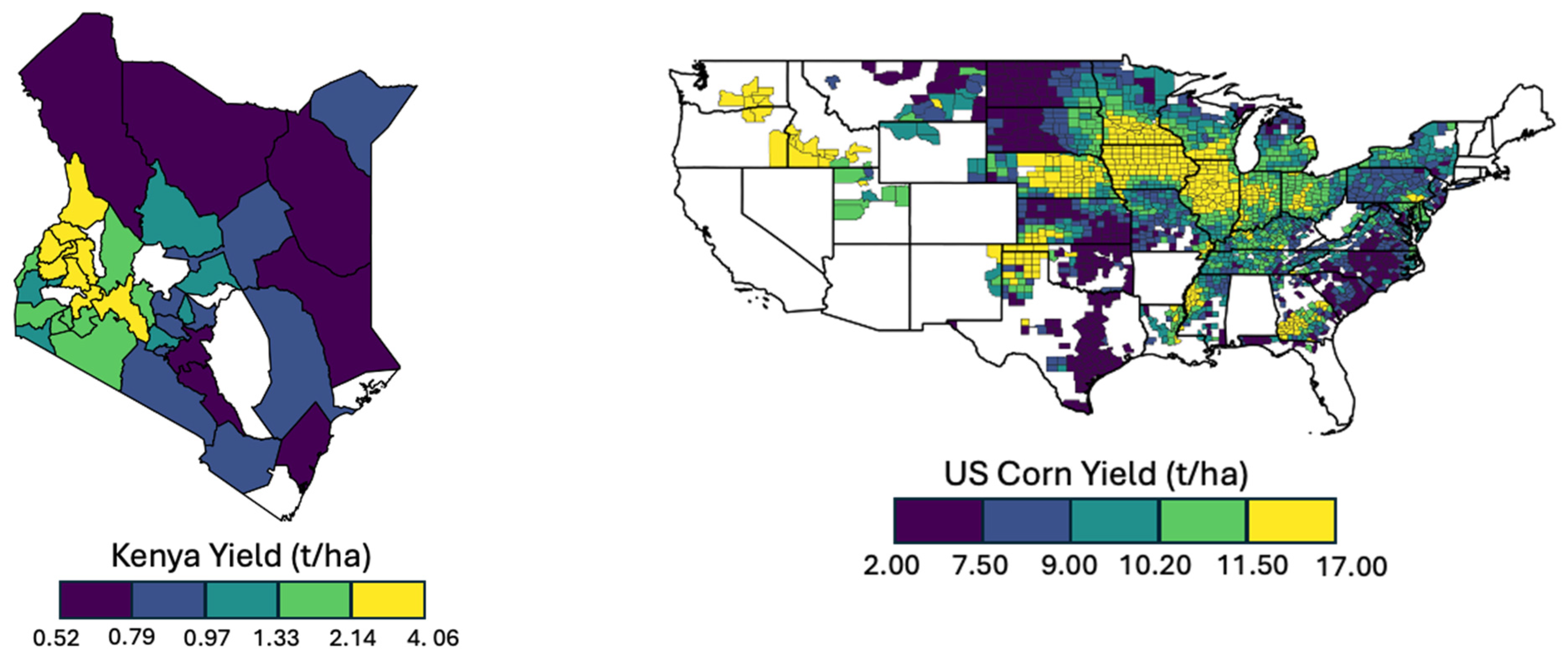
2.1. Study Areas and Yield Data

In the U.S., county-level yield data were directly acquired from the USDA National Agricultural Statistics Service (NASS), derived from farmer surveys [28]. The U.S. dataset contains yield data from 2008 to 2023, yielding a robust record of inter-annual variability. In the U.S. Corn Belt, farms tend to be large—around 178 ha on average—and counties typically produce about 11 t/ha of corn each year [29,30]. In Kenya, county-level (admin level 1) yield observations on corn productivity are from the Kenyan Ministry of Agriculture and Livestock Development (MoALD) through their open data platform, KilimoSTAT, for five years, 2019–2023 [31]. In contrast to the U.S., Kenyan fields are mostly small—under 1 ha per farm—and national maize yields hover around 1.6 t/ha annually [32,33]. For reference, as shown in Figure 1, corn yields exhibit strong spatial variation across both Kenya and the U.S., with high-yielding counties clustering in agriculturally intensive regions like western Kenya and the U.S. Corn Belt.

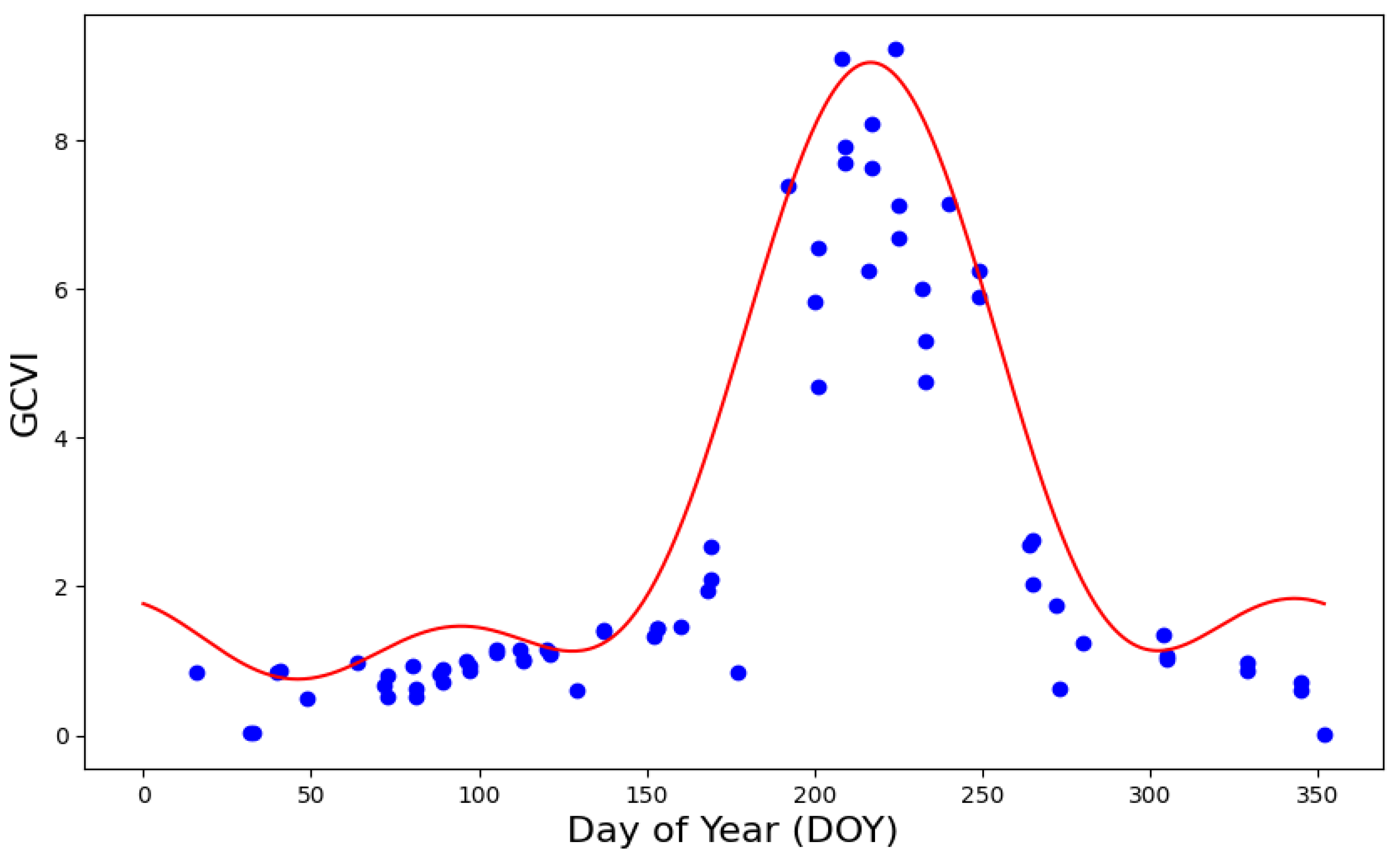
2.2. Satellite Data and Meteorologic Variables

The Sentinel-2 mission, launched in 2015 by the European Space Agency (ESA), collects optical imagery across 13 spectral bands from visible to short-wave infrared. It has a revisit time of 5 days and provides global coverage with a spatial resolution of up to 10 m [34]. We accessed the Sentinel-2 Level 2A data via Google Earth Engine (GEE) [35]. Specifically, cloud masking was implemented to remove pixels contaminated by clouds. Following that, crop-specific masks were applied to filter out irrelevant pixels. Specifically, the Cropland Layer (CDL) was used as the maize mask in the U.S. [36], and the ESA WorldCereal 10 m product was used in Kenya [37]. After that, the remaining pixels were aggregated to the county level by calculating the mean value within each county.

Following that, in both U.S. and Kenya, time-series Sentinel-2 data at the county level were collected from the first to the last day in each study year. On each observation date, two spectral bands, Near-Infrared (NIR) and Green, were retrieved from the satellite imagery and used to calculate the Green Chlorophyll Vegetation Index (GCVI), which measures the greenness of crops and is indicative of the productivity:

$$\mathrm{G}\mathrm{C}\mathrm{V}\mathrm{I}={\displaystyle \frac{\mathrm{N}\mathrm{I}\mathrm{R}}{\mathrm{G}\mathrm{R}\mathrm{E}\mathrm{E}\mathrm{N}}}-1$$

(1)

GCVI was chosen due to its sensitivity to changes in leaf chlorophyll content and reduced saturation effects compared to the frequently employed Normalized Difference Vegetation Index (NDVI) or Enhanced Vegetation Index (EVI) [38].

To interpolate the data temporally, a harmonic regression was applied and fitted to the time-series Sentinel-2 GCVI (Figure 2). Following that, we extracted critical values from the fitted harmonic curve: the peak GCVI in the growing season (GCVI_Peak), the GCVI 30 days before the peak (GCVI_b30), the GCVI 30 days after the peak (GCVI_a30), and the integral of GCVI between the peak and 30 days after the peak (GCVI_Int) [39]. These features capture a crop’s vegetative and reproductive growth phases. To ensure robust feature extraction, when multiple peaks were present in the harmonic regression curve, the maximum GCVI occurring within the defined growing-season window was selected as the peak value. In cases where no clear seasonal peak was identifiable, those observations were excluded from further analysis. This standardized procedure was applied uniformly across all counties and both countries to maintain consistency. The peak extraction method enhanced robustness by minimizing reliance on individual observation dates, enabling the consistent characterization of vegetation conditions across diverse spatial and temporal scales, especially in areas with fluctuating weather patterns and cloud cover. The quality of the extracted GCVI features depends on the appropriateness of the harmonic regression. To further illustrate the variability around the fitted harmonic curves, Supplementary Figure S3 presents examples of county-level GCVI time series with ±1 standard deviation ribbons for selected counties in Kenya and the U.S., highlighting the higher variance observed in the Kenyan data.

In addition, meteorological data from ERA5-Land were collected to reflect the climate conditions in the study areas [40]. Two meteorological variables were considered, including the monthly average temperature (Temp) and the monthly accumulative precipitation (PPT). Similarly, these meteorological variables were processed in GEE, including the implementation of crop-specific masks and spatial aggregation to the county level. As illustrated in Figure 2, the Sentinel-2 GCVI time series captures the seasonal vegetation dynamics, with a harmonic regression model fitted to smooth temporal fluctuations in a representative U.S. County. Finally, there are a total of 16 features for each county, including 4 Sentinel-2 features and 12 meteorological features (monthly Temp and PPT from April to September). These features were paired with the corresponding county yield records and ready for modeling.

3. Methodology

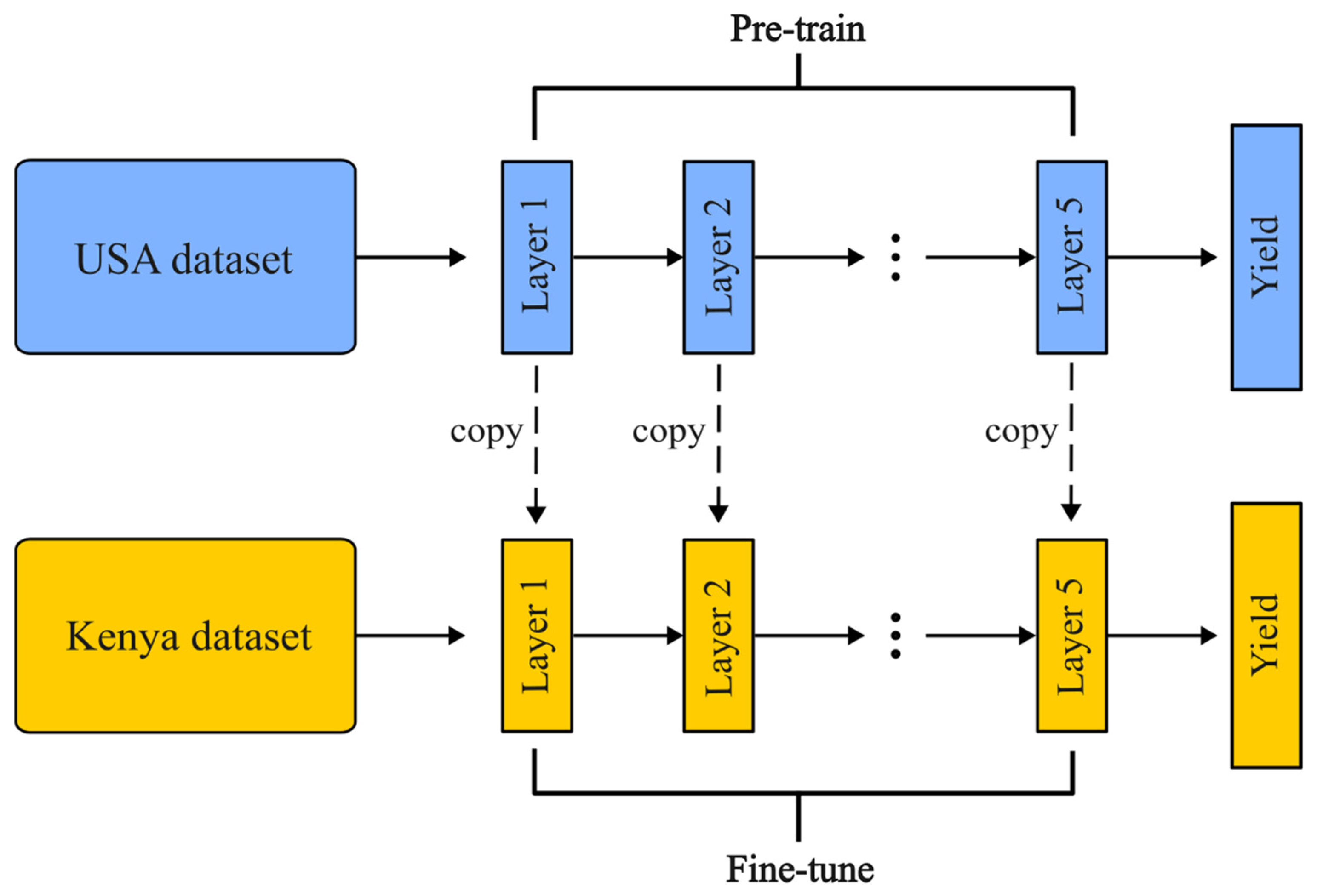
3.1. Fundamentals of Fine-Tuning-Based Transfer Learning

Though DNNs are extremely powerful, training them requires large amounts of labeled data, and this effect is exacerbated as the number of layers in the DNN increase due to the large number of parameters needed to make the network learn useful and informative features [41,42]. In the field of agriculture, it is not always practical to collect sufficient labeled data [43]. The lack of sufficient high-quality labeled datasets is a significant barrier for DNNs to be deployed and used in many applications in agriculture.

Another critical challenge in applying DNNs across different regions (domains) lies in domain shifts, which occur when the data distributions between two domains differ. Formally, a domain is defined as a feature space $\mathcal{X}$ and a marginal probability distribution $\mathrm{P}\left(\mathrm{X}\right)$ where $\mathrm{X}\in \mathcal{X}$. Domain shift occurs when the source domain and target domain are related but exhibit differences in their marginal distributions $\left({\mathrm{P}}_{\mathrm{S}}\left(\mathrm{X}\right)\ne {\mathrm{P}}_{\mathrm{T}}\left(\mathrm{X}\right)\right)$ even when their feature spaces are identical ${(\mathcal{X}}_{\mathrm{s}}={\mathcal{X}}_{\mathrm{T}})$ [44]. These shifts hinder the generalization of models trained in the source domain when deployed in the target domain [45].

Transfer learning (TL) is a powerful ML technique that has emerged to resolve the issue of domain shifts and to reduce deep learning’s dependence on training data. TL works by leveraging the abundance of data in ${\mathrm{D}}_{\mathrm{S}}$ to enhance model performance when applied to ${\mathrm{D}}_{\mathrm{T}}$. TL utilizes knowledge from a source domain and task (${\mathrm{D}}_{\mathrm{S}},{\mathrm{T}}_{\mathrm{S}})$ to improve the learning of a predictive function ${\mathrm{f}}_{\mathrm{T}}\left(·\right)$ in a target domain and task (${\mathrm{D}}_{\mathrm{T}},{\mathrm{T}}_{\mathrm{T}})$, wherein the source task and target task could be identical (${\mathrm{T}}_{\mathrm{S}},{\mathrm{T}}_{\mathrm{T}})$.

Fine-tuning-based transfer learning is one of the most used FT methods. It begins by pre-training a model on ${\mathrm{D}}^{\mathrm{S}}$ by minimizing a loss function ${\mathrm{L}}_{\mathrm{T}}\left({\mathrm{f}}_{\mathrm{T}}\left({\mathrm{X}}_{\mathrm{T}}\right),{\mathrm{Y}}_{\mathrm{T}}\right)$ for labeled data $\left({\mathrm{X}}_{\mathrm{T}},{\mathrm{Y}}_{\mathrm{T}}\right)\in {\mathrm{D}}_{\mathrm{T}}$. This pre-trained model is then fine-tuned on the target domain by minimizing a new loss function ${\mathrm{L}}_{\mathrm{T}}\left({\mathrm{f}}_{\mathrm{T}}\left({\mathrm{X}}_{\mathrm{T}}\right),{\mathrm{Y}}_{\mathrm{T}}\right)$ using labeled data $\left({\mathrm{X}}_{\mathrm{T}},{\mathrm{Y}}_{\mathrm{T}}\right)\in {\mathrm{D}}_{\mathrm{T}}$. This method is effective due to the transferability of learned representation. During pre-training, the model captures hierarchical features, where the earlier layers extract general patterns, whereas the later layers learn task-specific representation. It then reuses these general layers while adapting the later layers of the model to the specific characteristics of ${\mathrm{D}}_{\mathrm{T}}$, reducing the need for large amounts of labeled data in the target domain [46,47].

Fine-tuning also presupposes a certain relationship between domains such that the knowledge acquired in ${\mathrm{D}}^{\mathrm{S}}$ remains applicable to ${\mathrm{D}}^{\mathrm{T}}$. While the marginal distributions may differ $\left({\mathrm{P}}_{\mathrm{S}}\left(\mathrm{X}\right)\ne {\mathrm{P}}_{\mathrm{T}}\left(\mathrm{X}\right)\right)$, the shared underlying structure helps in effective knowledge transfer. This shared structure refers to similarities in the feature space between both domains. For example, in agricultural domains, the physiological relationships between variables such as crop yield and weather conditions (e.g., precipitation and temperature) will remain the same across domains, even if the specific distribution may differ. Leveraging these fundamental similarities helps fine-tuning adapt a pre-trained model to a new domain effectively with minimal labeled data [44,48]. We would like to note that fine-tuning relies on the assumption of shared physiological relationships between domains. While we do not formally quantify domain similarity here, future work could evaluate this assumption by training a domain discriminator to empirically assess feature-space alignment prior to fine-tuning.

3.2. Designed Fine-Tuning Architecture

The fine-tuning approach in this study utilizes a DNN consisting of an input layer, 3 hidden layers, and an output layer. Neighboring layers are fully connected layers. Each hidden layer is followed up by a ReLU (Rectified Linear Unit) activation function. The model is pre-trained on $D^S$ comprising 9296 U.S. samples. The pre-training is performed for 201 epochs using the MSE (Mean Squared Error) loss function and the Adam optimizer with a learning rate of 0.01. A weight decay regularization of 0.01 is used to prevent the model from overfitting. After pre-training, the model is fine-tuned on $D_T$, which consists of 157 Kenyan county-level data samples for the years 2019, 2020, and 2021, 158 samples for 2022, and 159 samples for 2023. The fine-tuning process runs for 150 epochs with a reduced learning rate of 0.001 and no regularization. Input features for both $D_T$ and $D_s$ include ERA5 precipitation and temperature data and Green Chlorophyll Vegetation Index (GCVI) values for a total of 11 time-series input features. Due to significant differences in the marginal distributions between the source and target domains, each dataset is scaled individually using separate scalers fitted to their respective data distributions.

Besides the fine-tuned DNN, we also established performance baselines by training upper-bound models and lower-bound models. An upper-bound model is trained and tested exclusively on the target domain, providing an estimate of the best possible performance achievable with the labeled data provided. In other words, the model is both trained and tested on the target domain. The accuracy is regarded as the upper bound since there are none of the domain shift issues mentioned before. In contrast, the lower-bound model is trained on the source domain and directly evaluated on the target domain, without any transfer learning or domain adaptation. Its accuracy is defined as the lower bound because no efforts have been put to address the domain shifts, leading to degraded performance.

Both upper- and lower-bound approaches include a DNN model and an RF model each, resulting in a total of four models. For the lower-bound models, input features from both the source and target domains are scaled using the same transformation to account for differences in feature distributions. The RF models were implemented using scikit-learn, a widely used ML library known for its efficient and accessible implementations [49]. The DNN models were developed using PyTorch 2.6.0, a Python-based deep learning framework [50]. All models were trained and tested on Google Colab, utilizing GPU acceleration to enhance computational efficiency. The workflow for the fine-tuned DNN model is shown in Figure 3.

3.3. Model Evaluation

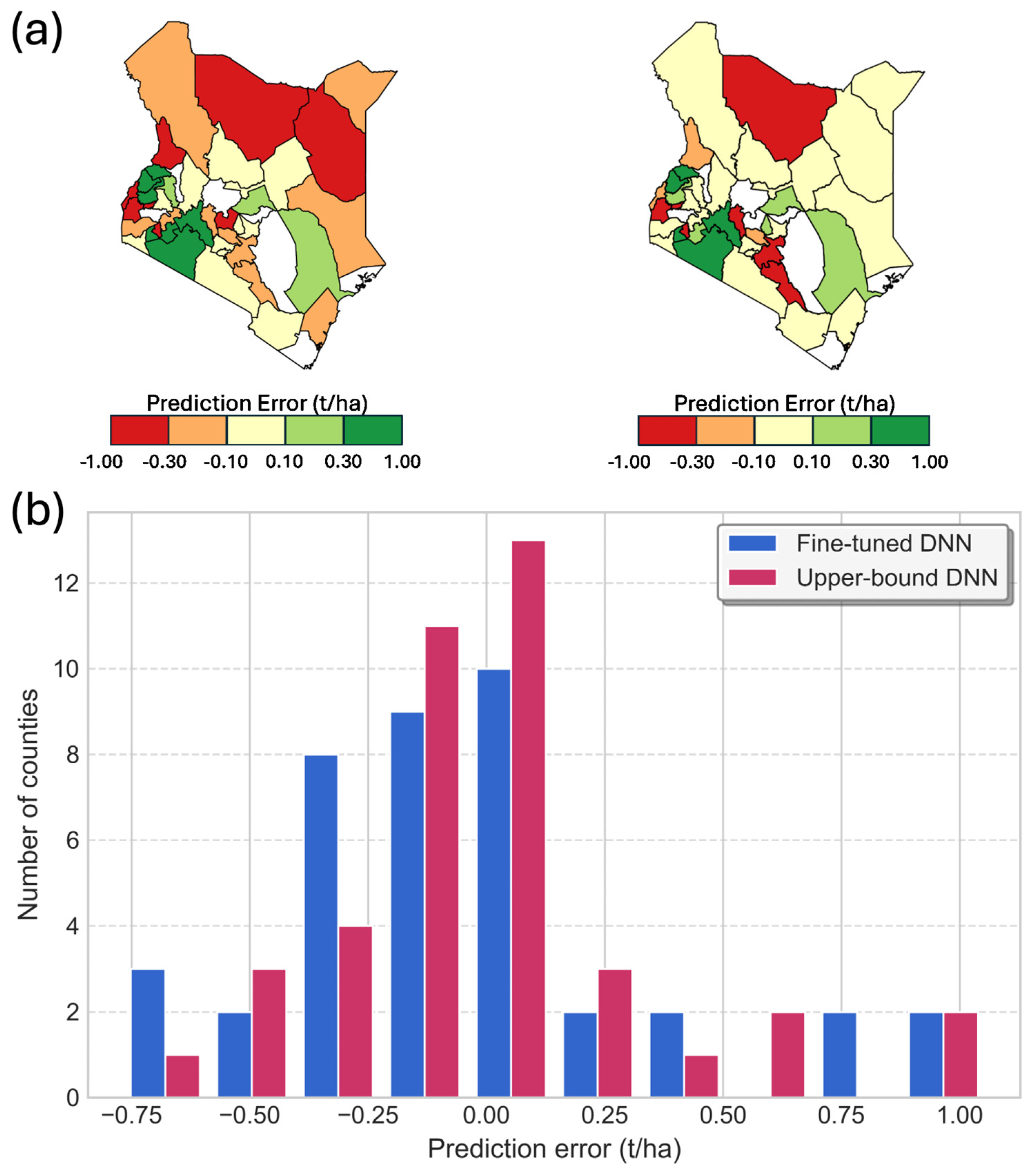
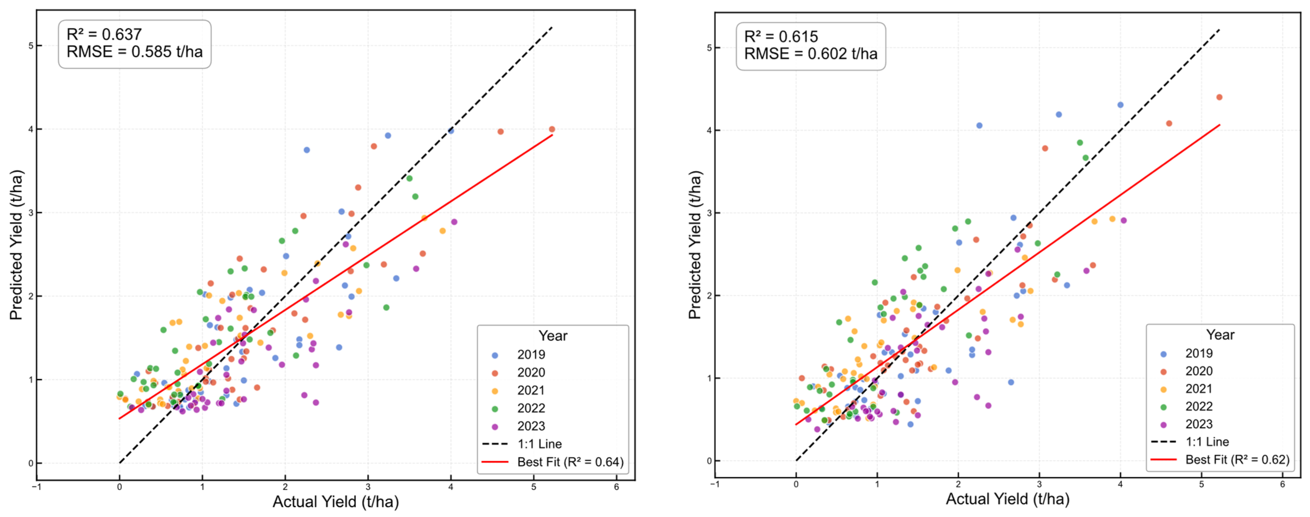
The fine-tuned model, alongside the lower- and upper-bound models, underwent evaluation in a transfer experiment from the U.S. to Kenya. We implemented leave-one-year-out cross-validation for all 3 models, where each model would be trained using 4 years of data and then evaluated using the last remaining year. In each cross-validation, the coefficient of determination (${\mathrm{R}}^2$) and root mean square error (RMSE) metrics were utilized to evaluate model performance:

$${\mathrm{R}}^2=1-{\displaystyle \frac{{\sum }_{\mathrm{i}=1}^{\mathrm{n}}{\left(\widehat{{\mathrm{y}}_{\mathrm{i}}}-{\mathrm{y}}_{\mathrm{i}}\right)}^2}{{\sum }_{\mathrm{i}=1}^{\mathrm{n}}{\left(\overline{\mathrm{y}}-{\mathrm{y}}_{\mathrm{i}}\right)}^2}}$$

(2)

$$\mathrm{R}\mathrm{M}\mathrm{S}\mathrm{E}=\sqrt{{\displaystyle \frac{1}{\mathrm{n}}}{\sum }_{\mathrm{i}=1}^{\mathrm{n}}{\left({\mathrm{y}}_{\mathrm{i}}-\widehat{{\mathrm{y}}_{\mathrm{i}}}\right)}^2}$$

(3)

where $\widehat{y_i}$ is the predicted yield by the models and $y_i$ is the corresponding reported yield; $\overline{y}$ is the average yield across all data samples; and n denoted the total number of samples in a given testing year.

4. Results

Table 1. Evaluation results of $R^2$ and RMSE (t/ha) for corn yield prediction in 2019–2023. The best performance is highlighted in bold.

Years	Number of Testing Samples	Fine-Tuned DNN		DNN				RF
				Upper-Bound		Lower-Bound		Upper-Bound		Lower-Bound
		${\mathit{R}}^{\mathbf{2}}$	RMSE	${\mathit{R}}^{\mathbf{2}}$	RMSE	${\mathit{R}}^{\mathbf{2}}$	RMSE	${\mathit{R}}^{\mathbf{2}}$	RMSE	${\mathit{R}}^{\mathbf{2}}$	RMSE
2019	40	0.607	0.572	0.566	0.601	−29.900	5.070	0.625	0.559	−5.140	2.260
2020	40	0.769	0.536	0.768	0.536	−22.100	5.370	0.685	0.626	−3.160	2.270
2021	40	0.637	0.581	0.682	0.543	−25.000	4.910	0.734	0.497	−5.070	2.370
2022	39	0.553	0.604	0.527	0.621	−30.000	5.000	0.389	0.706	−7.070	2.570
2023	38	0.404	0.647	0.328	0.687	−29.100	4.600	0.487	0.601	−5.900	2.200
Overall	197	0.632	0.589	0.618	0.598	−25.600	4.990	0.616	0.598	−4.800	2.330

presents the evaluation results for corn yield prediction for each testing year. Each experiment was repeated ten times, and the average $R^2$ and RMSE were reported for each case. The result with the highest evaluation accuracy for each case is highlighted in bold in Table 1.

To test whether the modest overall advantage of the fine-tuned DNN is robust, we performed paired t-tests and Wilcoxon signed-rank tests on county-level absolute errors across all years. No significant difference was found between the fine-tuned DNN and the upper-bound DNN (p > 0.6 for both tests), with mean absolute errors of 0.473 and 0.476 t/ha, respectively. Bootstrapped confidence intervals for RMSE and MAE further overlapped substantially, confirming that, on average, the two models perform equivalently. A year-by-year analysis showed that neither model consistently outperformed the other in 2019–2022. However, in 2023, the fine-tuned DNN achieved a statistically significant improvement (p = 0.008), suggesting that under certain annual conditions, cross-continental fine-tuning can yield meaningful gains. Notably, 2023 experienced widespread temperature anomalies across Kenya, with mean seasonal temperatures up to +1.7 °C above the five-year average. This warming may have made local conditions more similar to the U.S. source domain, helping the fine-tuned DNN better capture yield patterns under elevated heat stress. This gain in accuracy is consistent with the transfer learning improvements reported by Zhao et al., (2022), who likewise found that fine-tuned models outperformed local baselines when the weather differed from the training setting [26]. We additionally compared the fine-tuned DNN to the upper-bound RF model. On average across all years, their MAEs were nearly identical, and their RMSE/R² values overlapped in bootstrapped CIs, indicating no significant difference in overall accuracy. Year-by-year tests likewise showed no consistent winner in 2019–2023 (all p > 0.10). This further confirms that, on average, transfer-learned DNNs perform on par with traditional RF baselines—and can occasionally edge them out under certain seasonal conditions.

Besides the overall performance, both the fine-tuned DNN and upper-bound models had large year-to-year variance in their accuracies. This shows that while the upper-bound models can excel in some years, unexpected changes in the data distribution in certain years may pose challenges to their ability to generalize. It can also be seen that all three high-performing models (fine-tuned DNN, upper-bound DNN, and upper-bound RF) seem to have a lower accuracy in later years—2022 and 2023. This could be due to changes in climate and domain shifts that can lead to degraded performance. The upper-bound models, which are trained exclusively on the target domain, face the challenge of being trained on fewer than 200 rows in the dataset. Because of this limited training size, they might be overfitting to specific instances rather than learn robust patterns, leading to reduced performance when the data distribution shifts even slightly.

On the other hand, there are extremely negative R² values and high RMSE values among the lower-bound DNN and RF models (Table 1). These results illustrate that when trained solely on the source domain and tested directly on target data, the models can fail to generalize altogether, substantially underperforming naive baselines.

In Figure 4a, we present error maps from 2019 to 2023 for corn prediction, with colors closer to a darker shade of green indicating an error of 1 and colors closer to a darker shade of red indicating an error of −1. As shown in the figure, the improvements brought by fine-tuned DNN mainly happen to counties in southwestern areas. In the northern regions, the errors are slightly higher compared to the upper-bound DNN. The main reason is that northern regions have much lower yield, with most regions having a yield below 1 t/ha (Figure 1, left). This is much lower than most of counties in the U.S. (Figure 1, right). As such, data from the U.S. can be less informative. Nevertheless, fine-tuned DNN more effectively captures the underlying yield patterns across Kenya’s counties as demonstrated by the higher R². The spatial distribution of errors suggests that upper-bound DNN makes more conservative predictions with fewer overestimation errors but potentially fails to fully capture the inherent variability in the yield data. Figure 4b confirms that the errors are unnormalized raw differences (spanning –0.75 to +1.05 t ha⁻¹). The fine-tuned DNN (blue) shows a slightly wider spread and more underestimation than the upper-bound model (red), which helps explain its higher R² despite a small bias. Nakuru exhibits the largest overprediction, with an error = +1.057 t ha⁻¹, by the fine-tuned DNN. This county’s extensive, flat, commercial maize fields produce very uniform GCVI signals, which the model appears to interpret as higher yields. Vihiga shows the greatest underprediction, with an error = −0.770 t ha⁻¹. Its hilly, smallholder-dominated landscape results in mixed spectral responses that the DNN struggles to capture fully.

Finally, Figure 5 shows the scatterplot for predicted and actual yield values for the fine-tuned DNN and upper-bound DNN. The black dashed reference line represents a perfect prediction, where there is a 1:1 ratio between predicted and actual value. The red line presents the line of best fit. The scatter plots presented for fine-tuned DNN and upper-bound DNN highlight distinct strengths in their predictive performance. The upper-bound DNN model exhibits strong agreement with actual values in lower yield ranges (below 1 t/ha), which is consistent with the error maps (Figure 4). However, the scatters are more spread out and distant from the reference line. This indicates the underfitting of the model due to the limited training data in Kenya. The fine-tuned DNN, on the other hand, partially addresses the issue and achieves better overall agreement between the actual yields and the predicted yields.

5. Discussion

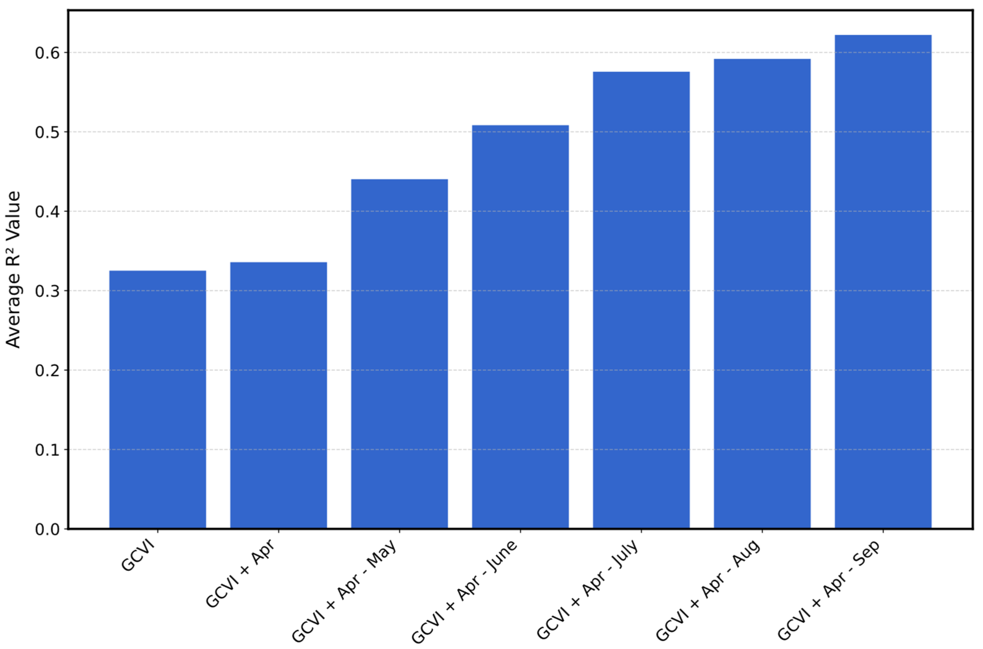
5.1. Feature Importance

We conducted a feature importance analysis of the fine-tuned DNN model to explore the relationship between different feature sets and the model accuracy. The fine-tuned DNN model was trained from scratch each time using the defined feature set, starting with only remote sensing (RS) features (i.e., GCVI_peak, GCVI_int, GCVI_b30, and GCVI_a30), and then progressively including the ERA5 weather data from April through September. Each combination was tested 10 times, and then the average of the R² values was taken. Figure 6 visualizes this trend, showing how model accuracy improves with each additional month of weather data, though the marginal gains taper off toward the end of the growing season.

An improvement in model performance is consistently observed as additional monthly weather data are incorporated with the baseline GCVI, underscoring the effectiveness of multi-feature integration. Notably, even with just the addition of April weather data, there is a slight improvement in average value, reaching approximately 0.33 compared to 0.32 when using only the baseline GCVI, though this may just be a stochastic event.

As more monthly weather data are integrated, the performance continues to improve significantly, rising from about 0.33 with GCVI + April to about 0.62 when the complete set of weather data through September is utilized. However, the incremental gains in performance seem to diminish as later months are added, with a marked difference in improvement rates: transitioning from April to May yields nearly a 0.11 increase in average value, while moving from August to September results in a modest improvement of about 0.03. The addition of May and June weather data provides particularly substantial gains, suggesting that these months capture critical environmental conditions relevant to the prediction task. This variation reflects the different impact of seasonal weather data, demonstrating that specific monthly combinations enable the model to better learn underlying patterns, adapt more effectively, and deliver improved outcomes. This trend suggests that the model not only becomes more accurate with more weather data but also exhibits different response patterns depending on which specific monthly information is incorporated, reinforcing the importance of weather data selection. The prominence of May–June weather features in our importance ranking agrees with Kang et al. (2020), who showed that early-season rainfall and temperature explain the majority of variance in Midwestern maize yields [5].

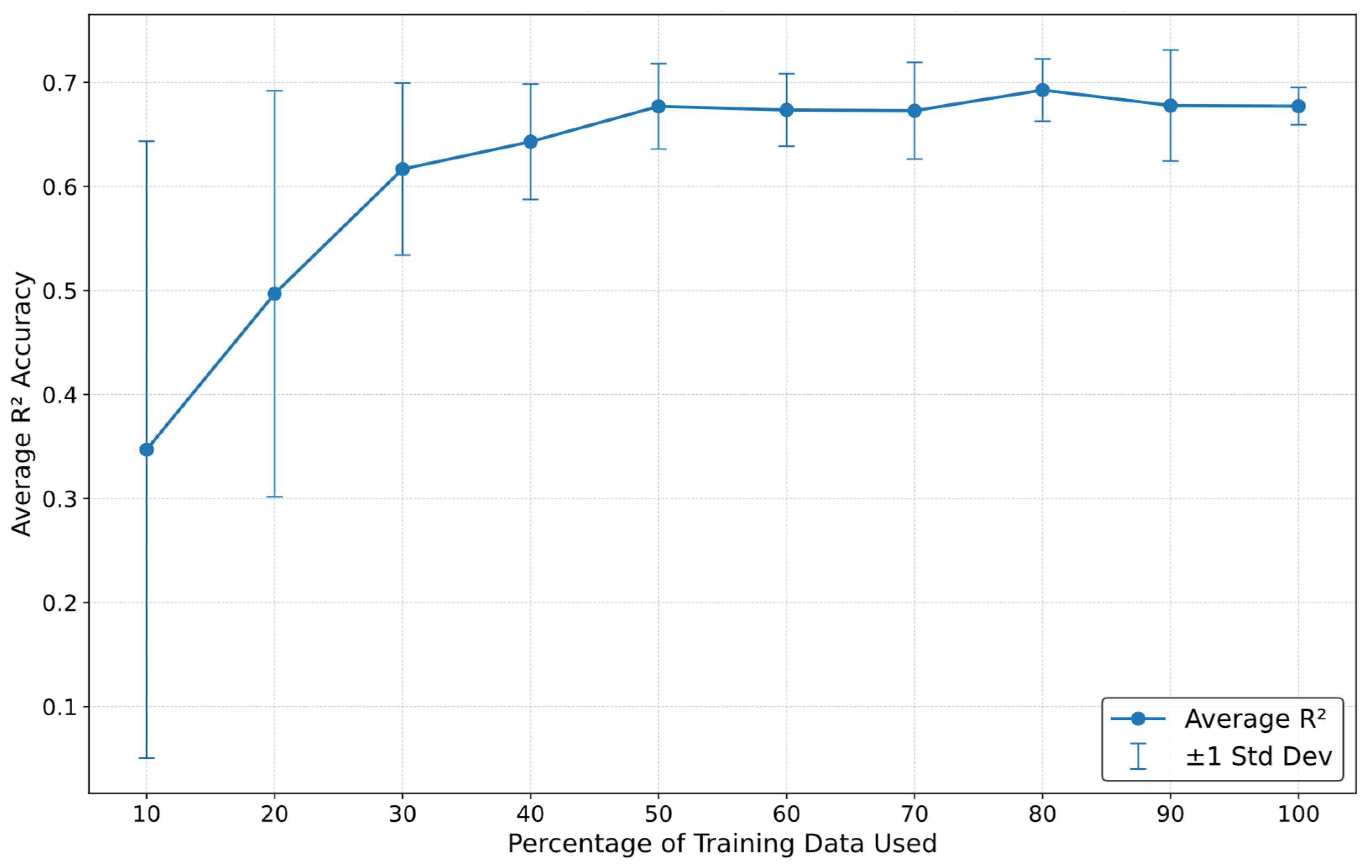
5.2. Sensitivity Analysis

We conducted a sensitivity analysis on the fine-tuned DNN model to examine the improvement in R² accuracy as a function of the percentage of target domain training data used during fine-tuning, taking 2020 as the representative test year. The model was first fine-tuned on all years of the pre-training data and then, after saving the weights, the model was fine-tuned using increasing percentages of training data. This was repeated over ten iterations, and the averages of the R² values were saved. To avoid yearly bias, the training data were randomized, and the first $\left(n\times 10\right)\mathit{\%}$ of the data were used for the $n^{th}$ iteration. Figure 7 illustrates this sensitivity, showing how the fine-tuned model’s performance improves with increasing percentages of target-domain training data.

An improvement in R² accuracy is consistently observed as the percentage of fine-tuning data increases, underscoring the effectiveness of transfer learning and highlighting the ability of the pre-trained model to leverage source domain knowledge for quick adaptation to the target domain. Notably, even with only 10% of the training data, there is a significant jump in accuracy, reaching approximately 0.35 compared to −0.25 when no fine-tuning is applied to the lower-bound DNN model.

As the percentage of training data increases, the accuracy continues to improve, rising from about 0.23 at 10% of training data to nearly 0.70 when 100% of the data are utilized. However, the incremental gains in accuracy diminish as more data are added, with a marked difference in improvement rates: transitioning from 20% to 30% of training data yields nearly more than a 0.1 increase in R² accuracy, while moving from 90% to 100% results in almost no change in accuracy. Additionally, the standard deviation of accuracy decreases as more training data are used. This reduction reflects greater stability in results across the 10 iterations, demonstrating that a larger dataset enables the model to better learn underlying patterns, adapt more effectively, and deliver consistent high-accuracy outcomes. This trend suggests that the model not only becomes more reliable with more data but also minimizes the variability in performance, reinforcing its robustness. This result is similar to that of Zhao et al., (2022), where fine-tuning achieved R² > 0.6 with roughly one-quarter of local wheat samples, underscoring the data-efficiency benefit of TL in smallholder systems [26].

5.3. Limitations and Future Work

Though this result is promising, this study has limitations and many ways it can be expanded upon. Firstly, the fine-tuning process was tested on a small test dataset from the target domain which may not accurately represent the true performance of the model in real-world scenarios. This arises due to the challenge of accessing diverse, larger datasets in data-scarce regions. However, having a large testing dataset goes against the main premise of transfer learning, which is to achieve high performance with a low amount of data. This trade-off highlights a fundamental challenge in evaluating models designed for such applications. The model’s performance could be influenced by overfitting to the small test dataset, as fine-tuning requires a delicate balance between learning from the source domain and adapting to the target domain. This potential overfitting could limit the model’s generalizability to unseen data. This study’s scope was limited to only the U.S. as the source domain and Kenya as the target domain. Though these regions have relatively different climate and agricultural practices, the study still may not capture the full range of challenges of applying transfer learning across other regions with diverse climatic and agricultural conditions. These observations reinforce the recent conclusion of Chang et al., (2024) that even large ‘foundation’ crop models require targeted adaptation when transferred across continents [27].

For future work, a simple way that this study could be expanded on would be to involve additional regions beyond U.S. and Kenya. For instance, selecting source and target domains with varying climatic conditions, such as tropical, temperate, or arid regions, or with distinct agricultural practices, crop varieties, or soil types could help understand the strength and limitations of this method further. Another way to expand on this could be to increase the size of the test set. More extensive data could better represent the wide range of environmental, climatic, and agricultural factors present in real-world settings, reducing the risk of skewed or overly optimistic performance estimates. They could include data from multiple growing seasons, different crop types, and regions with varying levels of data availability, which would not only help validate the robustness of the model but also help ensure that the model’s predictions are reliable under dynamic conditions.

6. Conclusions

ML and DL models have been increasingly used for crop yield prediction but are facing issues of data scarcity due to the requirement of large amounts of data for training. This is even less feasible in data-scarce, underdeveloped regions with low amounts of infrastructure for data collection. To tackle this issue, an effective strategy is to utilize fine-tuning-based TL which uses a source domain with a large amount of data to learn general patterns and then fine-tune the model on the target domain with a scarce dataset. In this study, we used this strategy to perform cross-continental fine-tuning-based TL and proposed a fine-tuned DNN model for crop yield estimation based on satellite-derived VIs and meteorological variables. Transfer experiments between two distinct ecological zones, namely, Kenya and the U.S., demonstrated that a fine-tuned DNN model can stabilize and improve yield prediction accuracies for the corn crop. The fine-tuned DNN model can potentially outperform commonly used supervised learning models (i.e., RF and DNN) with upper bounds being set as the model is trained only on the target domain and lower bounds as it is trained only on the source domain. This was achieved using data from 5 years (2019–2023) for the target domain and utilizing leave-one-year-out validation for testing accuracy. Model interpretation showed that pre-training and then fine-tuning the model allowed it to be more stable and be able to better adapt to the patterns of the data rather than memorizing them, leading to more inconsistent performance. Although this study has demonstrated the effectiveness of cross-continental fine-tuning-based TL for estimating crop yields, there are still several avenues for future research. One potential direction is to explore the scalability of fine-tuning-based TL for other crops and ecological zones with varying data availability. Another area for future investigation is the integration of fine-tuning techniques with advanced domain adaptation methods to further enhance model robustness and transferability in highly heterogeneous data environments [51,52].

References

1. Tigchelaar, M.; Battisti, D.S.; Naylor, R.L.; Ray, D.K. Future warming increases probability of globally synchronized maize production shocks. Proc. Natl. Acad. Sci. USA 2018, 115, 6644–6649. [Google Scholar] [CrossRef] [PubMed]
2. Shafi, U.; Mumtaz, R.; Anwar, Z.; Ajmal, M.M.; Khan, M.A.; Mahmood, Z.; Qamar, M.; Jhanzab, H.M. Tackling Food Insecurity Using Remote Sensing and Machine Learning-Based Crop Yield Prediction. IEEE Access 2023, 11, 108640–108657. [Google Scholar] [CrossRef]
3. Wang, Y.; Zhang, Z.; Feng, L.; Ma, Y.; Du, Q. A new attention-based CNN approach for crop mapping using time series Sentinel-2 images. Comput. Electron. Agric. 2021, 184, 106090. [Google Scholar] [CrossRef]
4. Lv, Z.; Huang, H.; Li, X.; Zhao, M.; Benediktsson, J.A.; Sun, W.; Falco, N. Land Cover Change Detection with Heterogeneous Remote Sensing Images: Review, Progress, and Perspective. Proc. IEEE 2022, 110, 1976–1991. [Google Scholar] [CrossRef]
5. Kang, Y.; Ozdogan, M.; Zhu, X.; Ye, Z.; Hain, C.R.; Anderson, M.C. Comparative assessment of environmental variables and machine learning algorithms for maize yield prediction in the US Midwest. Environ. Res. Lett. 2020, 15, 064005. [Google Scholar] [CrossRef]
6. Johnson, D.M. An assessment of pre- and within-season remotely sensed variables for forecasting corn and soybean yields in the United States. Remote Sens. Environ. 2014, 141, 116–128. [Google Scholar] [CrossRef]
7. Nguyen, L.H.; Robinson, S.; Galpern, P. Medium-resolution multispectral satellite imagery in precision agriculture: Mapping precision canola (Brassica napus L.) yield using Sentinel-2 time series. Precis. Agric. 2022, 23, 1051–1071. [Google Scholar] [CrossRef]
8. Awad, M.; Khanna, R. Deep Neural Networks. In Efficient Learning Machines; Apress: Berkeley, CA, USA, 2015; pp. 127–147. [Google Scholar] [CrossRef]
9. Cerulli, G. Fundamentals of Supervised Machine Learning: With Applications in Python, R, and Stata; Statistics and Computing; Springer International Publishing: Cham, Switzerland, 2023. [Google Scholar] [CrossRef]
10. Juang, B.H. Deep neural networks–A developmental perspective. APSIPA Trans. Signal Inf. Process. 2016, 5, 127–147. [Google Scholar] [CrossRef]
11. Balestriero, R.; Baraniuk, R. Deep Neural Networks. arXiv 2017, arXiv:1710.09302. [Google Scholar] [CrossRef]
12. Sun, J.; Di, L.; Sun, Z.; Shen, Y.; Lai, Z. County-Level Soybean Yield Prediction Using Deep CNN-LSTM Model. Sensors 2019, 19, 4363. [Google Scholar] [CrossRef]
13. Zhang, L.; Zhang, Z.; Luo, Y.; Cao, J.; Xie, R.; Li, S. Integrating satellite-derived climatic and vegetation indices to predict smallholder maize yield using deep learning. Agric. For. Meteorol. 2021, 311, 108666. [Google Scholar] [CrossRef]
14. Ma, Y.; Zhang, Z.; Kang, Y.; Özdoğan, M. Corn yield prediction and uncertainty analysis based on remotely sensed variables using a Bayesian neural network approach. Remote Sens. Environ. 2021, 259, 112408. [Google Scholar] [CrossRef]
15. Wang, Y.; Zhang, Z.; Feng, L.; Du, Q.; Runge, T. Combining Multi-Source Data and Machine Learning Approaches to Predict Winter Wheat Yield in the Conterminous United States. Remote Sens. 2020, 12, 1232. [Google Scholar] [CrossRef]
16. Lv, Z.; Zhang, P.; Sun, W.; Benediktsson, J.A.; Li, J.; Wang, W. Novel Adaptive Region Spectral–Spatial Features for Land Cover Classification with High Spatial Resolution Remotely Sensed Imagery. IEEE Trans. Geosci. Remote Sens. 2023, 61, 5609412. [Google Scholar] [CrossRef]
17. Sarron, J.; Beillouin, D.; Huat, J.; Koffi, J.; Diatta, J.; Malézieux, É.; Faye, E. Digital agriculture to fulfil the shortage of horticultural data and achieve food security in sub-Saharan Africa. Acta Hortic. 2022, 1348, 239–246. [Google Scholar] [CrossRef]
18. Jones, J.W.; Antle, J.M.; Basso, B.; Boote, K.J.; Conant, R.T.; Foster, I.; Godfray, H.C.J.; Herrero, M.; Howitt, R.E.; Janssen, S.; et al. Toward a new generation of agricultural system data, models, and knowledge products: State of agricultural systems science. Agric. Syst. 2017, 155, 269–288. [Google Scholar] [CrossRef]
19. Ma, Y.; Chen, S.; Ermon, S.; Lobell, D.B. Transfer learning in environmental remote sensing. Remote Sens. Environ. 2023, 301, 113924. [Google Scholar] [CrossRef]
20. Hilbert, M. Big Data for Development: From Information-to Knowledge Societies. SSRN Electron. J. 2013, 2205145. [Google Scholar] [CrossRef]
21. Kuria, A.W.; Bolo, P.; Adoyo, B.; Korir, H.; Sakha, M.; Gumo, P.; Mbelwa, M.; Orero, L.; Ntinyari, W.; Syano, N.; et al. Understanding farmer options, context and preferences leads to the co-design of locally relevant agroecological practices for soil, water and integrated pest management: A case from Kiambu and Makueni agroecology living landscapes, Kenya. Front. Sustain. Food Syst. 2024, 8, 1456620. [Google Scholar] [CrossRef]
22. Alvarado-Cárdenas, L.O.; Martínez-Meyer, E.; Feria, T.P.; Eguiarte, L.E.; Hernández, H.M.; Midgley, G.; Olson, M.E. To converge or not to converge in environmental space: Testing for similar environments between analogous succulent plants of North America and Africa. Ann. Bot. 2013, 111, 1125–1138. [Google Scholar] [CrossRef]
23. Hosna, A.; Merry, E.; Gyalmo, J.; Alom, Z.; Aung, Z.; Azim, M.A. Transfer learning: A friendly introduction. J. Big Data 2022, 9, 102. [Google Scholar] [CrossRef]
24. Tajbakhsh, N.; Shin, J.Y.; Gurudu, S.R.; Hurst, R.T.; Kendall, C.B.; Gotway, M.B.; Liang, J. Convolutional Neural Networks for Medical Image Analysis: Full Training or Fine Tuning? IEEE Trans. Med. Imaging 2016, 35, 1299–1312. [Google Scholar] [CrossRef] [PubMed]
25. Chew, R.; Rineer, J.; Beach, R.; O’neil, M.; Ujeneza, N.; Lapidus, D.; Miano, T.; Hegarty-Craver, M.; Polly, J.; Temple, D.S. Deep Neural Networks and Transfer Learning for Food Crop Identification in UAV Images. Drones 2020, 4, 7. [Google Scholar] [CrossRef]
26. Zhao, Y.; Han, S.; Meng, Y.; Feng, H.; Li, Z.; Chen, J.; Song, X.; Zhu, Y.; Yang, G. Transfer-Learning-Based Approach for Yield Prediction of Winter Wheat from Planet Data and SAFY Model. Remote Sens. 2022, 14, 5474. [Google Scholar] [CrossRef]
27. Chang, Y.-C.; Stewart, A.J.; Bastani, F.; Wolters, P.; Kannan, S.; Huber, G.R.; Wang, J.; Banerjee, A. On the Generalizability of Foundation Models for Crop Type Mapping. arXiv 2024, arXiv:2409.09451. [Google Scholar] [CrossRef]
28. United States Department of Agriculture, National Agricultural Statistics Service. Quick Stats Database. United States Department of Agriculture (USDA-NASS). 2025. Available online: https://quickstats.nass.usda.gov/ (accessed on 18 April 2025).
29. United States Department of Agriculture, National Agricultural Statistics Service. 2017 Census of Agriculture. USDA NASS. 2019. Available online: https://www.nass.usda.gov/Publications/AgCensus/2017/ (accessed on 21 April 2025).
30. Corn: United States Area, Yield, and Production. USDA Foreign Agricultural Service, PS&D Online. Available online: https://ipad.fas.usda.gov/countrysummary/Default.aspx?crop=Corn&id=US (accessed on 21 April 2025).
31. KilimoSTAT. Ministry of Agriculture and Livestock Development. Available online: https://statistics.kilimo.go.ke/en/ (accessed on 4 March 2025).
32. Food and Agriculture Organization of the United Nations. Family Farming Data Portrait–Kenya. Food and Agriculture Organization of the United Nations (FAO). Available online: https://www.fao.org/family-farming/data-sources/dataportrait/country-details/en/?cnt=KEN (accessed on 21 April 2025).
33. FAOSTAT (FAO). Kenya Maize Yield–FAOSTAT. FAOSTAT (Food and Agriculture Organization of the United Nations). Available online: https://www.fao.org/faostat/en/#data/QCL (accessed on 21 April 2025).
34. Drusch, M.; Del Bello, U.; Carlier, S.; Colin, O.; Fernandez, V.; Gascon, F.; Hoersch, B.; Isola, C.; Laberinti, P.; Martimort, P.; et al. Sentinel-2: ESA’s Optical High-Resolution Mission for GMES Operational Services. Remote Sens. Environ. 2012, 120, 25–36. [Google Scholar] [CrossRef]
35. Gorelick, N.; Hancher, M.; Dixon, M.; Ilyushchenko, S.; Thau, D.; Moore, R. Google Earth Engine: Planetary-scale geospatial analysis for everyone. Remote Sens. Environ. 2017, 202, 18–27. [Google Scholar] [CrossRef]
36. Boryan, C.; Yang, Z.; Mueller, R.; Craig, M. Monitoring US agriculture: The US Department of Agriculture, National Agricultural Statistics Service, Cropland Data Layer Program. Geocarto Int. 2011, 26, 341–358. [Google Scholar] [CrossRef]
37. Van Tricht, K.; Degerickx, J.; Gilliams, S.; Zanaga, D.; Battude, M.; Grosu, A.; Brombacher, J.; Lesiv, M.; Bayas, J.C.L.; Karanam, S.; et al. WorldCereal: A dynamic open-source system for global-scale, seasonal, and reproducible crop and irrigation mapping. Earth Syst. Sci. Data 2023, 15, 5491–5515. [Google Scholar] [CrossRef]
38. Ma, Y.; Liang, S.-Z.; Myers, D.B.; Swatantran, A.; Lobell, D.B. Subfield-level crop yield mapping without ground truth data: A scale transfer framework. Remote Sens. Environ. 2024, 315, 114427. [Google Scholar] [CrossRef]
39. Deines, J.M.; Patel, R.; Liang, S.-Z.; Dado, W.; Lobell, D.B. A million kernels of truth: Insights into scalable satellite maize yield mapping and yield gap analysis from an extensive ground dataset in the US Corn Belt. Remote Sens. Environ. 2021, 253, 112174. [Google Scholar] [CrossRef]
40. Copernicus Climate Change Service. ERA5-Land Monthly Averaged Data from 1950 to Present; Copernicus Climate Change Service (C3S) Climate Data Store (CDS): Brussels, Belgium, 2019. [Google Scholar] [CrossRef]
41. Alzubaidi, L.; Bai, J.; Al-Sabaawi, A.; Santamaría, J.; Albahri, A.S.; Al-Dabbagh, B.S.N.; Fadhel, M.A.; Manoufali, M.; Zhang, J.; Al-Timemy, A.H.; et al. A survey on deep learning tools dealing with data scarcity: Definitions, challenges, solutions, tips, and applications. J. Big Data 2023, 10, 46. [Google Scholar] [CrossRef]
42. Li, Y. Deep Learning with Very Few and No Labels. Ph.D. Thesis, University of Missouri--Columbia, Columbia, MO, USA, 2021. [Google Scholar] [CrossRef]
43. Wang, M.; Deng, W. Deep visual domain adaptation: A survey. Neurocomputing 2018, 312, 135–153. [Google Scholar] [CrossRef]
44. Cook, D.; Feuz, K.D.; Krishnan, N.C. Transfer learning for activity recognition: A survey. Knowl. Inf. Syst. 2013, 36, 537–556. [Google Scholar] [CrossRef] [PubMed]
45. Pan, S.J.; Yang, Q. A Survey on Transfer Learning. IEEE Trans. Knowl. Data Eng. 2010, 22, 1345–1359. [Google Scholar] [CrossRef]
46. Tan, C.; Sun, F.; Kong, T.; Zhang, W.; Yang, C.; Liu, C. A Survey on Deep Transfer Learning. arXiv 2018, arXiv:1808.01974. [Google Scholar] [CrossRef]
47. Alzubaidi, L.; Zhang, J.; Humaidi, A.J.; Al-Dujaili, A.; Duan, Y.; Al-Shamma, O.; Santamaría, J.; Fadhel, M.A.; Al-Amidie, M.; Farhan, L. Review of deep learning: Concepts, CNN architectures, challenges, applications, future directions. J. Big Data 2021, 8, 53. [Google Scholar] [CrossRef]
48. Weiss, K.; Khoshgoftaar, T.M.; Wang, D.D. A survey of transfer learning. J. Big Data 2016, 3, 9. [Google Scholar] [CrossRef]
49. Pedregosa, F.; Varoquaux, G.; Gramfort, A.; Michel, V.; Thirion, B.; Grisel, O.; Blondel, M.; Müller, A.; Nothman, J.; Louppe, G.; et al. Scikit-learn: Machine Learning in Python. arXiv 2012, arXiv:1201.0490. [Google Scholar] [CrossRef]
50. Paszke, A.; Gross, S.; Massa, F.; Lerer, A.; Bradbury, J.; Chanan, G.; Killeen, T.; Lin, Z.; Gimelshein, N.; Antiga, L.; et al. PyTorch: An Imperative Style, High-Performance Deep Learning Library. arXiv 2019, arXiv:1912.01703. [Google Scholar] [CrossRef]
51. Ma, Y.; Zhang, Z.; Yang, H.L.; Yang, Z. An adaptive adversarial domain adaptation approach for corn yield prediction. Comput. Electron. Agric. 2021, 187, 106314. [Google Scholar] [CrossRef]
52. Ma, Y.; Yang, Z.; Huang, Q.; Zhang, Z. Improving the Transferability of Deep Learning Models for Crop Yield Prediction: A Partial Domain Adaptation Approach. Remote Sens. 2023, 15, 4562. [Google Scholar] [CrossRef]
Figure 1. (Left): The average corn yield map in Kenya (2019–2023). (Right): The average corn yield map in the U.S. (2008–2023). A lighter color indicates a higher yield value for the county. State and county names are provided in Supplementary Figures S1 and S2.
Remotesensing 17 01717 g001
Figure 2. The time series Sentinel-2 GCVI (blue) and the fitted harmonic regression curve (red) in Adams County, Illinois, USA.
Remotesensing 17 01717 g002
Figure 3. The workflow of the fine-tuning-based transfer learning (FTL). The model is first pre-trained on the source U.S. dataset and then fine-tuned on the target dataset from Kenya.
Remotesensing 17 01717 g003
Figure 4. (a) County-level error map for the fine-tuned DNN model (left) and upper-bound DNN model (right). Error is calculated as the raw (unnormalized) difference between predicted and reported yields (t ha−1), where negative values indicate overestimation and positive values indicate underestimation. County names are provided in Supplementary Figure S1. (b) Histogram of county-level prediction errors (predicted–observed, t ha−1) for the fine-tuned DNN (blue) and upper-bound DNN (red).
Remotesensing 17 01717 g004
Figure 5. Scatter plot of fine-tuned DNN model (left) and upper-bound DNN (right) comparing predicted and actual yield values.
Remotesensing 17 01717 g005
Figure 6. Averaged R2 values on fine-tuned DNN model trained and evaluated using leave-one-year-out cross validation on years 2019–2023, across 10 iterations.
Remotesensing 17 01717 g006
Figure 7. Line plot with error brackets to represent the sensitivity of the fine-tuned DNN model with the percentage of training data used to train in 2020.
Remotesensing 17 01717 g007