Abstract
Riparian vegetation reduces the conveyance capacity and increases the likelihood of floods. Studies that consider vegetation in flow modeling rely on unmanned aerial vehicle (UAV) data, which restrict the covered area. In contrast, this study explores advances in remote sensing and machine learning techniques to obtain vegetation data for an entire river by relying solely on satellite data, superior to UAVs in terms of spatial coverage, temporal frequency, and cost effectiveness. This study proposes a machine learning method to obtain key vegetation parameters at a resolution of 10 m. The goal was to evaluate the applicability of remotely sensed vegetation data using the proposed method on a dynamic roughness distributed runoff model in the Abukuma River to assess the effect of vegetation on the typhoon Hagibis flood (12 October 2019). Two machine learning models were trained to obtain vegetation height and density using different satellite sources, and the parameters were mapped in the river floodplains with 10 m resolution based on Sentinel-2 imagery. The vegetation parameters were successfully estimated, with the vegetation height overestimated in the urban areas, particularly in the downstream part of the river, then integrated into a dynamic roughness calculation routine and patched into the RRI model. The simulations with and without vegetation were also compared. The machine learning models for density and height obtained fair results, with an R2 of 0.62 and 0.55, respectively, and a slight overestimation of height. The results showed a considerable increase in water depth (up to 17.7% at the Fushiguro station) and a decrease in discharge (28.1% at the Tateyama station) when vegetation was considered.
1. Introduction
River management involves controlling the river environment to ensure both the ecological health of the river and the safety of nearby populations against flooding. Flood modeling is employed to predict the outcomes of flood events, from which decision-makers can propose flood control strategies. To provide reliable results, hydraulic models are dependent on a series of input parameters such as topography, flow data, and roughness in the river channel and surrounding areas [1]. The roughness value depends on several factors, such as surface irregularities, cross-sectional shape, obstructions, river meandering, and vegetation and flow conditions [2]. With significant variability in parameters, models often require a calibration process to determine the correct roughness value.
During channel overflow, the riparian vegetation present in the floodplain areas is the dominant factor determining the roughness value [3]. Large plants with rigid branch structures cause obstructions and diversions on the flow path [4], whereas smaller plants, such as tall grass species and shrubs, have a more complex interaction with flow dynamics, expressed by altering Manning’s roughness value. In the literature, the methods used to determine the roughness values due to vegetation are usually separated depending on whether the vegetation is emergent [5,6,7,8,9,10] or submerged [3,9,11,12,13,14,15]. For emergent vegetation, the most important physical property used to determine the Manning value is vegetation density. In this case, a common practice is to apply the frontal area of the vegetation as a density parameter to calculate the Manning value [9,16,17]. This practice can be useful for one-dimensional analysis, but it is difficult to apply to two-dimensional models. The leaf area index (LAI) is another parameter that can be used as a density descriptor [8]. The LAI is defined as the total one-sided leaf area over a ground unit, and it was first proposed for roughness calculation in emergent vegetation by Järvelä [5]. For submerged vegetation, the roughness can be obtained from the effective water depth, which is the ratio of water depth to plant height [13,15,18]. It is important to note that other factors also influence the roughness value, like the branch structure, stem flexibility, and foliage [6,14,19,20,21,22]. Assuming a constant Manning value does not properly comprehend the effect of vegetation on flow dynamics because, in flood events, the roughness value changes with variations of flow and vegetation conditions. Developing models capable of dynamically calculating the roughness based on these variations can generate more accurate results than those using a static roughness setting [3].
Regardless of its importance, considering vegetation in flood simulations is not common practice because of difficulties in obtaining vegetation data for broad areas. Advances in remote sensing have addressed these issues. Vegetation data have been successfully acquired and monitored using different remote sensing techniques, such as 3D point cloud data obtained from unmanned aerial vehicles (UAVs) [23,24,25] and satellite imagery [24,26,27,28,29,30,31,32,33,34,35]. UAV-3D point cloud data have advantages over satellite imagery, generating 3D terrain models with higher resolution that are independent of atmospheric conditions. However, satellite imagery has a higher temporal resolution and can cover broader areas than UAVs, which can only generate data on a localized scale. Moreover, satellites are equipped with a large number of sensors, enabling the calculation of numerous vegetation indices (VIs) [36] that have a strong relationship with vegetation parameters [37].
Recently, the combination of satellite data and machine learning has become popular in scientific research. This strategy has proven to be effective for acquiring important vegetation parameters within large areas [24,28,30,32]. The downscaling of vegetation LAI from coarse-resolution satellite products like MODIS to high resolution through combining Sentinel-2-derived VIs and machine learning was successfully performed by Gokool et al. [32], and later, a similar approach was applied by Fortes et al. [24] for flood simulation. Moreover, the combination of localized satellite lidar technology with satellite optical and synthetic aperture radar images and machine learning led to the extrapolation and mapping of canopy height over broad areas with high resolution by Li et al. [30]. Using a similar strategy, Lang et al. [28] developed a global canopy height model for 2020 with Sentinel-2 resolution on the Google Earth Engine (GEE) platform. These breakthroughs in technology have expanded the possibilities of using vegetation data from various locations worldwide for multiple purposes.
Previous studies that considered vegetation for roughness calculations typically relied on UAV data to obtain the vegetation parameters, as reported by Yoshida et al. [38] and Fortes et al. [24,25]. However, UAVs can only cover limited areas; therefore, these studies have been restricted to small river sections. In contrast, this study proposes a novel approach for obtaining vegetation parameters that relies solely on satellite data. This allows for the analysis of broader areas, with this study focusing on the entire core part of the main river within a catchment.
The primary objective of this study is to evaluate the applicability of satellite and machine learning-derived vegetation parameters to a dynamic vegetative roughness routine in a distributed runoff model. The secondary objectives were (1) to develop a machine learning technique to obtain vegetation parameters with 10 m resolution from satellite images, (2) to develop a dynamic roughness routine that considers vegetation LAI and height, and (3) to assess the effect of floodplain vegetation on flow dynamics.
2. Study Area
In Japan, rivers are classified as Class A (longer rivers managed by the national government) or Class B (shorter rivers managed by local governments). The research was conducted in the Abukuma River, a Class A river that flows through the Fukushima and Miyagi prefectures in the Tohoku region of Japan. The river originates at Asahidake and flows downstream through the valley formed by the Ou Mountains to the west and the Abukuma Plateau to the east. The river is 239 km long, and with a catchment area of 5390 km2, it has the second largest catchment in the region [39]. Figure 1 shows the location of the catchment with four observation stations along the river mainstream: Akutsu, Fukushima, Fushiguro, and Tateyama stations.
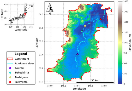
Figure 1.
Map of the Abukuma catchment showing the catchment elevation, the Abukuma river centerline, and 4 water level gauge stations.
Approximately 1.36 million people reside within the catchment, with the river flowing through Koriyama and Fukushima, two of the most populated cities in Fukushima prefecture. On 12 October 2019, Typhoon Hagibis struck the Abukuma Catchment. In upper Abukuma (upstream from Fukushima station), the event caused a total of 31 levee breaches, the inundation of approximately 12,000 households, and the deaths of 19 people [40]. The typhoon also caused immense damage in lower Abukuma; for example, in Marumori town in Miyagi Prefecture, 983 houses were inundated, of which 113 were destroyed [41]. In addition to Typhoon Hagibis, the catchment experienced severe flood events in 1986 and 1998.
3. Materials and Methods
The effect of vegetation on flow dynamics was evaluated by comparing the results of two different simulations. One simulation considered vegetation height and LAI to dynamically calculate the Manning value, referred to here as the dynamic model (DM), while another simulation considered a static Manning value, the static model (SM). Two machine learning models were developed to estimate the LAI and vegetation height in the Abukuma River floodplain.
3.1. Mapping Vegetation Parameters
Mapping vegetation parameters with 10 m resolution is essential for their application in flood modeling. At the catchment scale, vegetation is important for several processes during rainfall events, such as interception and evapotranspiration; however, from a hydraulic perspective, the interaction between flow and vegetation mostly occurs within floodplain areas. Therefore, for flood modeling, data with higher resolution are necessary to express the conditions of vegetation with the required level of detail in a much narrower space.
Downscaling of coarse-resolution satellite LAI products was performed across the entire Abukuma catchment area, and extrapolation of spatially sparse vegetation height from satellite LiDAR products was conducted in areas close to the Abukuma River.
3.1.1. LAI Downscaling
The relationship between the LAI and satellite VIs was explored to map the LAI in the Abukuma catchment at the required resolution. The normalized difference vegetation index (NDVI) is the most widely explored VI in remote sensing for LAI estimation [29,31,37,42]. The NDVI is the normalized ratio between the red and near-infrared (NIR) bands and characterizes vegetation growth and health [36]. Despite its usefulness, the NDVI tends to saturate in areas with high vegetation biomass [43]. The enhanced vegetation index (EVI) differs from the NDVI in correcting for soil and atmospheric effects [36], resulting in a less saturated index in those areas. Thus, relating both NDVI and EVI to LAI in machine learning has proven to be an effective strategy for LAI downscaling [32]. A schematic of the LAI downscaling model is shown in Figure 2.
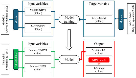
Figure 2.
The scheme of the LAI model training and prediction.
The dataset used for training the LAI model was obtained from MODIS products with a 500 m resolution over the entire Tohoku region of Japan. MODIS LAI (MOD15A2H V6, 8-day temporal resolution), MODIS NDVI, and EVI (MOD13A1 V6, 16-day temporal resolution) images were collected from July to September (Japan’s summer season) in 2020, and the median of each variable was calculated. LAI was used as the target variable, and NDVI and EVI were used as input variables to train a random forest regressor (RF) model. The scikit-learn 1.3.2 Python package [44] was used to train the model, which was trained with 300 estimators; all other parameters remained at their default values from the package. Figure 3 shows a map of the median images for all variables from the MODIS satellite images.
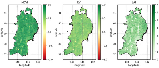
Figure 3.
Median image of the MODIS VIs and LAI used in the LAI model, calculated with the images collected from July to September of 2020.
With the trained model, LAI downscaling was performed by applying the NDVI and EVI calculated from Sentinel-2 with a 10 m resolution. For this purpose, a Sentinel-2 Level-2A mosaic scene from 15 September 2019 was used. This image was selected because of its low cloud coverage and proximity to the simulated event dates.
A raw downscaled LAI map was masked to remove LAI values predicted within the river channel area. The normalized difference water index (NDWI) is similar to the NDVI, which normalizes the ratio of the blue and NIR bands. The index values range from −1 to 1, where values above 0 indicate inland water bodies. The NDWI was calculated using the Sentinel-2 image and used to remove the LAI values where water bodies were present.
3.1.2. Vegetation Height Extrapolation
Launched in 2018, the ICESat-2 satellite emits three parallel pairs of laser beams onto the surface spaced approximately 3 km apart, with each pair containing a strong and a weak beam that is used to detect surfaces of high and low reflectivity. It detects photons that are geolocated with X and Y coordinates and receives a height value Z calculated from the photon travel time to the satellite [45]. The satellite’s main objective was to take measurements of ice caps in land and sea environments, but it demonstrated significant spatial details in the surface profiles of different types of environments, including vegetated land [46], thus providing the ATL08 product, which contains measurements of surface topography and vegetation canopy height. The algorithm applied to the ATL08 product labels the photons as ground or canopy photons; then, approximately 140 photons are used to calculate the product parameters inside footprints with a diameter of 17 m spaced 100 m along the track beams. When fewer than 50 labeled photons are available in a footprint, no calculation is performed [45]. Restricted to the footprint, the canopy height data from the ATL08 product lack continuous spatial distribution. A machine learning model was trained to extrapolate the height of the vegetation to the areas within the river floodplain. A scheme explaining all processing steps of the model can be observed in Figure 4.
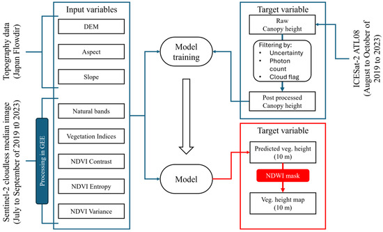
Figure 4.
The scheme of the vegetation height model training and prediction.
The model considers topography and spectral data as input parameters. The spectral data were obtained from a 10 m resolution median cloudless composite calculated from all Sentinel-2 satellite Level-2A images during the summer season (July, August, and September) from 2019 to 2023. Calculations were performed using the GEE platform [47]. Except for the B2, B3, B4, and B8 bands, the B5, B6, B7, B8A, B10, and B11 bands were resampled to a 10 m resolution with bicubic interpolation. Natural bands from the median image were used as the input parameters for the model. In addition, a series of VIs were calculated from the composite image, along with the contrast, entropy, and variance texture features of the NDVI, which were added to the input variables. The calculated VIs and their formulas are listed in Table 1. The topographic data considered in the model were obtained from the Japan Flow Direction dataset with an original resolution of 30 m [48]. A digital elevation model (DEM) was used to calculate the aspect and slope, and three variables were included in the machine learning model.

Table 1.
List of VIs and their formulas used as input variables of the vegetation height model.
The ICESat-2 ATL08 product contains ten canopy height profile quantiles: the 25th, 50th, 60th, 70th, 75th, 80th, 85th, 90th, 95th, and 98th percentile heights. The 98th percentile canopy height above the center coordinates of the footprints was chosen as the canopy height value for training the model. Data were collected from 2019 to 2023 and from August to October. The collected data were preprocessed using a set of threshold values for the key parameters. Footprints with canopy and ground uncertainties above 2 m were removed, as were footprints with fewer than 40 canopy photons or fewer than 50 ground photons. In addition, footprints with cloud flag 2 or higher were removed. A total of 52,700 footprints were collected, and 1507 footprints remained after preprocessing.
Figure 5 shows the locations of the selected ATL08 footprints after preprocessing on the RGB image of a cloudless composite. The coordinates at the center of the footprints were used to determine the pixels in each image of the input variables. Prior to the unification of the dataset, each input variable image was normalized based on its minimum and maximum values.
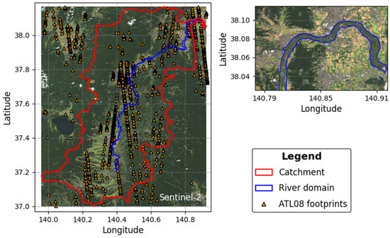
Figure 5.
Map of the Sentinel-2 RGB median cloudless composite with the ATL08 footprints used in the model on top, showing the borders of the Abukuma catchment, and the river domain area.
The model was trained using the RF algorithm, which has been shown to yield accurate predictions in previous studies [30,49,50,51]. The model was trained with 1000 estimators, a minimum of 50 samples to split the nodes, and a minimum of 10 samples per leaf. The model is trained using the scikit-learn package in Python [44].
Because of the large number of input variables, extrapolation was performed only in the river domain areas, which comprised the terrain between the river embankments, to reduce computational cost, as shown in Figure 5. To estimate vegetation height in these areas, the spectral and topographic variables were unified in a tabular format. Due to the difference in resolution, the pixel coordinates of the cloudless composite images were used to obtain the values of the topographic variables for each pixel, and the vegetation height was extrapolated. With vegetation height values present within the river channel area, the NDWI was used to mask these values, similar to LAI downscaling. This process was conducted separately for each area.
3.2. RRI Model
The typhoon event was simulated using the RRI model [52,53,54], a two-dimensional model capable of simulating rainfall-runoff and inundation phenomena simultaneously. The model calculates the processes in slope areas and rivers separately using a 2D diffusive wave model for the slope cells and a 1D diffusive wave model for the river cells. The governing equations of the model are the continuity and momentum equations, as shown in Equations (1)–(3):
where is the water surface height, is the time, and are unit width discharges, and and are the velocities in and directions, is the rainfall, is the infiltration rate, is the water height from the datum, is the gravitational acceleration, and are the shear stress in and directions, and is the water density.
The model requires topography, land cover, rainfall, and roughness parameters in the slope areas and river channels as basic inputs. The topography data used as inputs were obtained from the MERIT hydrologically adjusted topography dataset [55]. The dataset is available at a 3 arc-seconds resolution, approximately 90 m at the equator. For the simulations, the data were resampled to a 9 arc-second resolution (approximately 270 m).
Land cover data were obtained from the Ministry of Land, Infrastructure, and Tourism (MLIT) in 2014. The land classes were reclassified into forests, small vegetation, water bodies, and buildings. Land cover affects the roughness and infiltration parameters of slope areas. Table 2 lists the parameters adopted for each land class, with the roughness parameter selected to be within the suggested range for each surface type [56]. The rainfall data used in the model were radar/rain gauge-analyzed (RA) precipitation data [57]. The dataset contained distributed rainfall data with a resolution of 1 km, collected over 48 h starting on 12 October 2019. Figure 6 shows the distributed accumulated rainfall over the catchment, the hourly rainfall hyetograph, and total accumulated rainfall.
Table 2.
Input parameters considered for each land class for the RRI simulations.
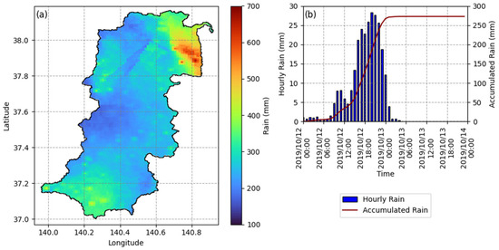
Figure 6.
Rainfall of the Typhoon Hagibis event: (a) The distributed accumulated rainfall in the Abukuma catchment; (b) The hourly and total accumulated rainfall.
The RRI model creates a rectangular cross-section for each river cell where no surveyed cross-sections are available. The model calculates the width and depth of the cross-section based on the contributing area of the cell. In this case, a single Manning value was set for all river cells. A Manning value of 0.022 was adopted for the river cells, where no surveyed cross-sections were set. A total of 864 cross-sections, spaced 200 m apart, were added to the model in the Abukuma River, as well as in the confluence areas of five tributaries: the Hirose, Surikami, Matsu, Sasahara, and Shakado Rivers. Figure 7 shows the river network of the catchment, with the stretches covered by the surveyed cross-sections.
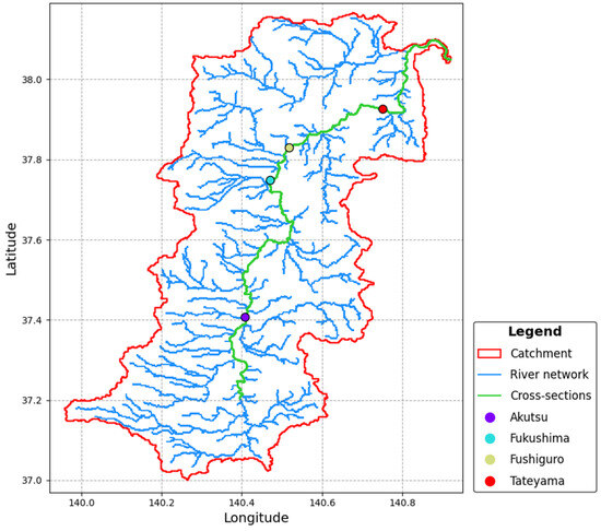
Figure 7.
Map of the river network showing the part of the rivers where cross-sections are available.
All parameters adopted for the slope areas and river cells without surveyed cross-sections were the same for the DM and SM. The only parameter that differed between the models was the Manning value adopted for the surveyed cross-sections. For the SM, a value of 0.022 was applied along the entire cross-sectional perimeter. For the DM, the channel and floodplains were discretized for each cross-section, with a Manning value of 0.022 adopted at the channel perimeter. In the floodplains, roughness was dynamically calculated at each time step using the LAI and vegetation height.
3.2.1. Dynamic Roughness Routine
The RRI model was patched with a dynamic roughness routine acting on the floodplains of the surveyed cross-sections. The routine calculates the Manning values for each cross-section and each time step under two different scenarios: emergent and submerged vegetation.
In the emergent vegetation scenario, the roughness calculation begins when the water depth reaches the floodplain height. At this stage, vegetation density is the primary factor for defining the roughness value. Considering the LAI as a measurement of density [8], the parameter is used to calculate the friction factor with the formula proposed by Järvelä [5], as shown in Equation (4).
where is the Darcy–Weisbach friction factor, is a species-specific parameter, is the drag coefficient of a leafy bush or tree species, is the flow velocity, is the lowest flow velocity used in determining , is the flow depth, and is the vegetation height. The ratio of flow depth to vegetation height expressed as assumes that the vegetation has a uniform LAI distribution, which decreases the total LAI value to the amount of vegetation that is in contact with the water.
The formula is applicable only for emergent vegetation, when and when . In the routine patched to the model, the value of was set to be equal to when lower than the latter. The adopted values of , , and were −1.03, 0.33, and 0.1, respectively, which are the values for the Black poplar species [6], a deciduous species chosen due to its range of LAI values.
The Darcy–Weisbach friction factor was converted to Manning’s roughness coefficient () using a process similar to that used by Box et al. [22], using the conversion formula shown in Equation (5).
Because the value of refers only to the Manning value in floodplains, it is combined with the channel Manning value into a single value using Equation (6):
where is the unified Manning value, is the channel Manning value, and are the floodplain and channel perimeters, respectively, and is the total perimeter of the cross-section.
When the flow depth exceeds the vegetation height, the submerged scenario routine is applied. In this routine, the degree of vegetation submergence is used to determine the Manning value [24,25]. The formulae proposed by Fortes et al. [25] were derived by unifying the observed relationship between the Manning coefficient and several types of vegetation in Japan under a single curve with exponential regression, as shown in Equation (7):
where . The formula produces a maximum Manning value of approximately 0.1 when the vegetation is barely submerged, while the minimum approaches 0.023. Similar to the emergent scenario, after calculating the floodplain Manning, Equation (6) was used to unify the Manning value. For both scenarios, whenever , .
3.2.2. Cross-Sections Vegetation Parameters
To run the DM, vegetation parameters were assigned to each cross-section based on the coordinates of the cross-sectional points. Figure 8 shows a stretch of the Abukuma River with the cross-sectional points overlayed in red.
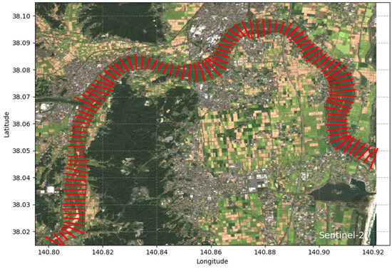
Figure 8.
Downstream part of the river with the cross-sections’ lines marked in red on top.
The values of LAI and vegetation height for each point of a cross-section were obtained from the vegetation parameter images generated by the two machine learning models. The points where either of the parameters was absent (e.g. in the river channel) were removed, and each parameter of the remaining points was averaged, resulting in a single LAI and vegetation height across the floodplains of each cross-section.
The floodplain height of each cross-section was determined based on the height of the lowest point at which both parameters were present. This procedure was effective for most cross-sections, but manual adjustment of the floodplain height was required for some sections.
4. Results
4.1. Vegetation Estimation Results
Machine learning models for LAI and vegetation height were trained and used to predict parameters in the target area. The values predicted from the test samples of each model were compared with the source values, and the coefficient of determination (R2) was calculated. Additionally, error metrics for each model were calculated, as listed in Table 3. A comparison between the predicted and observed values for the test samples is shown in the confusion plot in Figure 9, along with the sample density.
Table 3.
Metrics calculated from the test sample of each model.
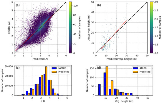
Figure 9.
Model results: (a) LAI model confusion plot with density of test samples; (b) Veg. height model confusion plot with density of test samples; (c) The histogram of MODIS and predicted LAI values of the test sample; (d) The histogram of ATL08 and predicted vegetation height of the test sample.
The MODIS LAI values range from 0 to 10, and within the study area, these values ranged from 0 to no higher than 7. Therefore, the RMSE obtained from the LAI model was considered acceptable. Figure 9a shows a higher density of points in the region where the predicted and MODIS LAI values were closest. For the vegetation height model, the RMSE of 5.5 m was achieved, and as shown in Figure 9b, the sample density was low in most parts of the graph. There were insufficient samples with values above 20 m.
The machine learning models were applied to the entire river floodplain areas to spatially estimate the vegetation parameters. The map of the vegetation parameters downstream of the river is shown in Figure 10.
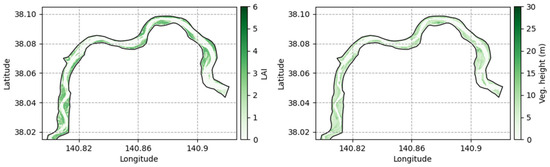
Figure 10.
Maps of predicted vegetation parameters in the floodplains downstream of the Abukuma River.
The values of LAI and vegetation height for each cross-section were calculated by averaging the parameter values located in the cross-sectional floodplains. To further validate the vegetation height model, the vegetation height at each cross-section was calculated from a high-resolution global canopy height model recently made available on the GEE platform [28]. Figure 11 shows the LAI and vegetation height values for both sources along the river’s length. The average predicted LAI and vegetation height across all cross-sections were 2.2 and 14 m, respectively.
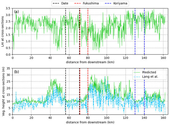
Figure 11.
Vegetation parameters at the cross-sections from downstream to upstream Abukuma river, the vertical lines show the location of the major cities the river passes through: (a) LAI values calculated for each cross-section; (b) Vegetation height calculated for each cross-section from the predicted map and from the global canopy height model from Lang et al. [28].
4.2. Simulation Results
The typhoon event could be simulated using both the SM and DM. Figure 12 shows the water depth and discharges obtained from both simulations along with a comparison with the observed measurements at the four gauge stations used for validation. The Nash–Sutcliffe coefficient and RMSE of the simulated depths and discharges at each gauge station were calculated to evaluate the accuracy of the SM and DM simulations. The results for depth and discharge are shown in Table 4 and Table 5, respectively. The variation in Manning’s roughness coefficient at each simulation hour due to changes in flow and vegetation conditions at Akutsu station is shown in Figure 13.
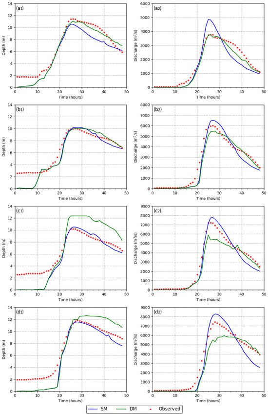
Figure 12.
Simulation results at each gauge station. Observed and simulated depths and discharges from the SM and DM at: (a1,a2) Akutsu, (b1,b2) Fukushima, (c1,c2) Fushiguro, and (d1,d2) Tateyama.
Table 4.
Nash–Sutcliffe and RMSE of the depths at each station for the SM and DM models.
Table 5.
Nash–Sutcliffe and RMSE of the discharges at each station for the SM and DM models.
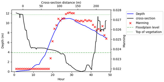
Figure 13.
Simulated Manning’s roughness coefficient variation caused by changes in vegetation and flow conditions at Akutsu station from the DM model.
Vegetation caused an increase in water depth at most stations, with increases of 4.8%, 17.7%, and 9.18% at the Akutsu, Fushiguro, and Tateyama stations, respectively, while a 1.5% decrease was simulated at the Fukushima station. In contrast, the discharge was considerably reduced by 22.4%, 15.9%, 24.2%, and 28.1% at the Akutsu, Fukushima, Fushiguro, and Tateyama stations, respectively.
The difference in simulated water levels between the SM and DM resulted in differences in inundation depth and area. The simulated inundation from the SM and DM in Date City is shown in Figure 14.
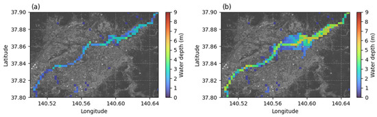
Figure 14.
Simulated inundation in Date City by the (a) SM model and (b) DM model.
5. Discussions
5.1. Vegetation Parameters in the Floodplains
The LAI model developed in this study considers the relationship of both EVI and NDVI with LAI values. The R2 of 0.62 was found within the mid position of the range achieved by Gokool et al. [32], with R2 between 0.38 and 0.94 and R from 0.62 to 0.97 with the application of a similar methodology to various study areas with homogeneous vegetation species.
The correlation between different VIs and LAI varies according to vegetation type and species [33,43]. Previously, LAI mapping was performed in patches of the same vegetation type [31,33]. In this study, the model was trained across a large area with a heterogeneous distribution of vegetation, unifying several vegetation types when establishing the VI–LAI relationships. This explains the position of the obtained R2 when placed within the range reported by Gokool et al. [32].
Given the range of LAI values within the study area (0–7), an RMSE of 0.52 obtained from the model suggests that the error in LAI prediction is within an acceptable range for the purposes of this research. In addition, the higher density of points where the predicted and MODIS LAI values were closest, as shown in Figure 9a, indicate that the model was capable of making accurate predictions for most samples.
The vegetation model achieved a fair correlation between the predicted and ATL08 vegetation height values, with an R2 of 0.55, within the range reported in previous studies [30,49,50,51], where canopy height extrapolation with the ICESat-2 satellite dataset was performed using data from all available periods. In this study, the data were collected only for the summer months, and a considerably smaller number of training samples were used, which could explain the lower coefficient of determination. Similar to Sothe et al. [51], the model overestimated short vegetation and underestimated tall trees.
Similar to the case of the LAI model, there is a considerable number of vegetation types in the study area, and the correlation between the input parameters and the vegetation height is also species-specific. Xi et al. [49] applied vegetation type classification to the inputs of the model, which could improve the results in areas with vegetation heterogeneity. The RMSE of 5.5 m was comparable to the value of 5.4 m reported by Sothe et al. [51] but higher than those of other studies [30,49,50]. Nevertheless, in this research, the vegetation height values were averaged for each cross-section, and the average absolute difference between the observed and predicted test samples was 0.4 m. Therefore, the result was considered acceptable for the purposes of this research.
As shown in Figure 11a, where the vegetation parameters are presented along the Abukuma river, it is evident the LAI values had a significant range of variation across the river length, however showing no significant change in pattern from urbanized to non-urbanized areas. In Figure 11b, despite the considerable variation, vegetation height was significantly lower in urbanized areas. Comparing the vegetation height calculated from the predicted map with that from Lang et al. [28], which reported an average vegetation height of 10 m, the predicted values were overestimated along the entire river; however, the pattern of variation in the values was very similar.
5.2. Vegetation Effect
Both the SM and DM simulations achieved good results and simulated the event with acceptable precision. The results of the simulations indicate that considering the vegetation in the river floodplains to dynamically calculate the Manning values based on density and height led to significant changes in the simulated depths and discharges at several locations when compared to the traditional approach of adopting a static Manning coefficient. The alterations in the simulated depth and discharge caused by variations in the Manning values led to an increase in simulation precision at specific stations, in agreement with Ebrahimi et al. [3]. The Nash–Sutcliffe coefficients shown in Table 4 demonstrate that depths simulated by both the SM and DM achieved good results, except for the depth simulated at Fushiguro station by the DM. Regarding the discharges, the DM achieved better results than the SM at the two upstream stations.
Dynamic vegetative manning values caused an increase in the simulated depth at most stations, as shown in Figure 12. According to Tabacchi et al. [4], vegetation in floodplains increases water retention in these areas, thereby increasing the water depth. From a more fundamental perspective, previous studies have shown that increasing hydraulic resistance due to riparian vegetation reduces flow velocities, causing water to back up and increase in depth [5,16,17]. The Manning behavior observed in Figure 13 demonstrates that the roughness increased during the emergent state of the riparian vegetation. This behavior has also been discussed in Aberle and Järvelä [6], who emphasized the importance of emergent vegetation in the increase in roughness, provoking flow deceleration and consequently the increase in water depth. Similarly, Nepf’s findings [7] indicate that vegetation drag, and turbulence significantly affect water depth, especially in regions with dense vegetation. However, in the submerged state of the vegetation, the value tends to decrease as the degree of submergence increases, as found by Nepf [7] and Wu et al. [9], who noted that as the vegetation becomes more submerged, the drag exerted by the vegetation decreases, decreasing the roughness and its effect on the flow conditions.
The simulated discharges from the DM and SM models demonstrated a reduction in discharge when vegetative roughness was considered, as shown in Figure 12. This discharge reduction supports the findings of other studies showing that increased hydraulic resistance reduces the flow rate, such as Cowan [2], Wu et al. [9] and Luhar and Nepf [20], indicating a significant increase in the hydraulic resistance effect on the reduction in the channel conveyance capacity and discharge. Additionally, Nikora et al. [15] noted the reduction of discharge in small streams, particularly in stretches with higher vegetation density, discussing the concept of “effective flow area reduction”, where the presence of vegetation reduces the available flow area, lowering the discharge. In addition, Ebrahimi et al. [3] also noted that a higher amount of vegetation increases hydraulic resistance and reduces discharge, regardless of whether it is submerged or emergent. Huthoff et al. [10] added that this effect is more evident during flood events because the flow becomes more confined, and the resistance increases.
The increase in water depth produced by the DM resulted in inundations that were not simulated by the SM. During Typhoon Hagibis, inundations occurred in Date City, just north of Fukushima. Figure 14 shows the inundation simulated by the SM and DM in Date City.
Different from studies that used the drag force of the vegetation to calculate the hydraulic resistance [7,14,19,21], this research explored the vegetation density described by the LAI [8] and used the index to calculate Manning’s roughness coefficient with the equation proposed by Järvelä [5]. As discussed by Jalonen et al. [8], there is great heterogeneity in vegetation density and distribution across floodplains, which can be observed by the variation in LAI values in different patches of vegetation in the river floodplains, as shown in Figure 10. Fortes et al. [24] used the LAI approach to calculate roughness in a 2D hydraulic model and achieved improvements in accuracy. The use of a 2D model can better capture the spatial variations in vegetation density; however, in this research, the RRI model was adopted, which applies 1D modeling in the river domain, where the LAI and vegetation height were averaged for each cross-section, and the same species-specific coefficients required for Equation (4) were adopted for all the river cross-sections. Thus, this approach lacks a detailed understanding of the spatial distribution of vegetation characteristics, potentially leading to low accuracy.
However, 2D models have a higher computational cost; thus, they are often applied to restricted stretches of rivers, using upstream discharge as the hydraulic data input. The application of a discharge that does not account for vegetation overestimates the flow feed of the model and may lead to an overestimation of the results. For future research, the application of vegetation data in 2D models at the catchment scale could address the issue of flow rate feed and simultaneously consider spatial variations in vegetation in floodplain areas.
Another key factor to consider in this study is the overestimation of vegetation height in the floodplains compared to the vegetation height reported by Lang et al. [28], as previously discussed and shown in Figure 11. This vegetation height overestimation may have delayed the stage at which the submerged scenario routine was activated, thereby delaying the calculation of the roughness with a decreasing trend. This may have limited the expected decrease in roughness, potentially preventing a slight increase in water depth and a less pronounced decrease in discharge. This is clearly demonstrated in Figure 13, where the water depth did not surpass the top of the vegetation at any point in the simulation. This hypothesis is aligned with the idea that a higher vegetative roughness provoked by a prolonged emergent state delays the transition to a smoother flow condition, impacting the depth and discharge at various locations.
For effective river management, incorporating riparian vegetation into flood modeling through the dynamic Manning strategy can significantly enhance model accuracy, resulting in more precise flood hazard maps. Furthermore, the constant changes in vegetation due to seasonal shifts and vegetation cutting impose the consideration of multiple scenarios of vegetation, which can provide a deeper understanding of the flood phenomena at a local level. This allows for optimized vegetation management; for instance, maintaining higher vegetation density upstream can reduce downstream flow rates, delaying peak flow. In addition, near-real-time vegetation data can improve early warning systems, enhancing flood risk prediction. Traditional flood control structures, such as levees and dikes, can be better designed to account for changes in vegetation distribution along the river.
By focusing on global satellite datasets, the methodology can be applied to different regions worldwide. However, there are limitations that should be carefully considered, such as the overestimation of vegetation height in urban areas, which can cause overestimation of the roughness.
6. Conclusions
In this study, LAI and vegetation height were mapped within the Abukuma River floodplain areas with 10 m resolution using two different machine learning models. The LAI model achieved good results, with R2 of 0.62 and RMSE of 0.52. These values are comparable with previous research on the subject, despite the more heterogeneous vegetation distribution in the study area, hindering the model performance. The vegetation height model achieved an R2 of 0.55 and an RMSE of 5.5 m, which is also comparable to previous research. Compared to previous studies, the model was trained with a lower number of training samples owing to the targeted ICESat-2 data collection during the vegetation growing season. In addition, similar to the LAI model, the high heterogeneity of vegetation types might have hindered the model’s performance. A comparison of the vegetation height values from the model predictions with those from a global canopy height model [28] demonstrated an overestimation of vegetation height at the floodplain level. In the future, using vegetation type classification in the study area might improve the performance of both the LAI and vegetation height models.
A dynamic Manning calculation routine was successfully patched to the RRI model based on the LAI and vegetation height values at the river cross-sections. The vegetative Manning value was routinely calculated at each time step based on the variations in vegetation and flow conditions. Two different simulations were performed: one without considering vegetation (SM) and one considering vegetation (DM). Comparisons between the SM and DM models showed that incorporating the vegetation caused a considerable decrease in discharge and an increase in water depth, resulting in inundation in areas where the SM model did not produce, but which actually occurred. The DM achieved a better performance at some locations in the upstream part of the catchment. Uncertainties related to the vegetation parameters at the cross-sections, especially the vegetation height, may have hindered the accuracy by overestimating the vegetative Manning values in some locations, which led to a higher impact downstream. Future research considering more accurate vegetation parameters may yield more accurate results. The use of 2D models capable of simulating at a catchment scale with higher resolution in the channel and floodplains could also improve the accuracy by accounting for the spatial variability of the vegetation parameters in the floodplains. The use of the dynamic Manning routine under different vegetation scenarios enables a deeper understanding of floods at a local level. River management authorities should consider the impact of vegetation on flow dynamics for the adoption of flood control strategies, such as optimized cutting of the vegetation and more precise delineation of flood hazard maps.
Author Contributions
Conceptualization, A.A.F. and M.H.; methodology, A.A.F.; software, A.A.F.; validation, A.A.F., M.H. and K.U.; formal analysis, A.A.F.; investigation, A.A.F.; resources, M.H. and K.U.; data curation, A.A.F.; writing—original draft preparation, A.A.F.; writing—review and editing, A.A.F., M.H. and K.U.; visualization, A.A.F.; supervision, M.H. and K.U.; project administration, M.H. and K.U.; funding acquisition, M.H. All authors have read and agreed to the published version of the manuscript.
Funding
This is a product of research which was financially supported in part by the Kansai University Fund for Supporting Young Scholars, 2025. “Real-Time Vegetation Observations for Enhanced Water Level Prediction in Small Rivers”.
Data Availability Statement
The original contributions presented in the study are included in the article, further inquiries can be directed to the corresponding author.
Acknowledgments
The authors acknowledge and appreciate the cross-sectional data of the Abukuma River provided by the Ministry of Land, Infrastructure, Transport, and Tourism (MLIT).
Conflicts of Interest
The authors declare no conflicts of interest.
References
- Bates, P.D. Remote Sensing and Flood Inundation Modelling. Hydrol. Process 2004, 18, 2593–2597. [Google Scholar] [CrossRef]
- Cowan, W.L. Estimating Hydraulic Roughness Coefficients. Agric. Eng. 1956, 37, 473–475. [Google Scholar]
- Ebrahimi, N.G.; Fathi-Moghadam, M.; Kashefipour, S.M.; Saneie, M.; Ebrahimi, K. Effects of Flow and Vegetation States on River Roughness Coefficients. J. Appl. Sci. 2008, 8, 2118–2123. [Google Scholar] [CrossRef][Green Version]
- Tabacchi, E.; Lambs, L.; Guilloy, H.; Planty-Tabacchi, A.-M.; Muller, E.; Décamps, H. Impacts of Riparian Vegetation on Hydrological Processes. Hydrol. Process 2000, 14, 2959–2976. [Google Scholar] [CrossRef]
- Järvelä, J. Determination of Flow Resistance Caused by Non-submerged Woody Vegetation. Int. J. River Basin Manag. 2004, 2, 61–70. [Google Scholar] [CrossRef]
- Aberle, J.; Järvelä, J. Flow Resistance of Emergent Rigid and Flexible Floodplain Vegetation. J. Hydraul. Res. 2013, 51, 33–45. [Google Scholar] [CrossRef]
- Nepf, H.M. Drag, Turbulence, and Diffusion in Flow through Emergent Vegetation. Water Resour. Res. 1999, 35, 479–489. [Google Scholar] [CrossRef]
- Jalonen, J.; Järvelä, J.; Aberle, J. Leaf Area Index as Vegetation Density Measure for Hydraulic Analyses. J. Hydraul. Eng. 2013, 139, 461–469. [Google Scholar] [CrossRef]
- Wu, F.-C.; Shen, H.W.; Chou, Y.-J. Variation of Roughness Coefficients for Unsubmerged and Submerged Vegetation. J. Hydraul. Eng. 1999, 125, 934–942. [Google Scholar] [CrossRef]
- Huthoff, F.; Augustijn, D.C.M.; Hulscher, S.J.M.H. Analytical Solution of the Depth-averaged Flow Velocity in Case of Submerged Rigid Cylindrical Vegetation. Water Resour. Res. 2007, 43, w06413. [Google Scholar] [CrossRef]
- Nepf, H.; Ghisalberti, M. Flow and Transport in Channels with Submerged Vegetation. Acta Geophys. 2008, 56, 753–777. [Google Scholar] [CrossRef]
- Devi, T.B.; Kumar, B. Experimentation on Submerged Flow over Flexible Vegetation Patches with Downward Seepage. Ecol. Eng. 2016, 91, 158–168. [Google Scholar] [CrossRef]
- Wang, P.; Wang, C.; Zhu, D.Z. Hydraulic Resistance of Submerged Vegetation Related to Effective Height. J. Hydrodyn. 2010, 22, 265–273. [Google Scholar] [CrossRef]
- Wilson, C.A.M.E. Flow Resistance Models for Flexible Submerged Vegetation. J. Hydrol. 2007, 342, 213–222. [Google Scholar] [CrossRef]
- Nikora, V.; Larned, S.; Nikora, N.; Debnath, K.; Cooper, G.; Reid, M. Hydraulic Resistance Due to Aquatic Vegetation in Small Streams: Field Study. J. Hydraul. Eng. 2008, 134, 1326–1332. [Google Scholar] [CrossRef]
- Baptist, M.J.; Babovic, V.; Rodríguez Uthurburu, J.; Keijzer, M.; Uittenbogaard, R.E.; Mynett, A.; Verwey, A. On Inducing Equations for Vegetation Resistance. J. Hydraul. Res. 2007, 45, 435–450. [Google Scholar] [CrossRef]
- Nepf, H.M. Flow and Transport in Regions with Aquatic Vegetation. Annu. Rev. Fluid. Mech. 2012, 44, 123–142. [Google Scholar] [CrossRef]
- Anderson, B.G.; Rutherfurd, I.D.; Western, A.W. An Analysis of the Influence of Riparian Vegetation on the Propagation of Flood Waves. Environ. Model. Softw. 2006, 21, 1290–1296. [Google Scholar] [CrossRef]
- Västilä, K.; Järvelä, J. Modeling the Flow Resistance of Woody Vegetation Using Physically Based Properties of the Foliage and Stem. Water Resour. Res. 2014, 50, 229–245. [Google Scholar] [CrossRef]
- Luhar, M.; Nepf, H.M. From the Blade Scale to the Reach Scale: A Characterization of Aquatic Vegetative Drag. Adv. Water Resour. 2013, 51, 305–316. [Google Scholar] [CrossRef]
- Jalonen, J.; Järvelä, J. Estimation of Drag Forces Caused by Natural Woody Vegetation of Different Scales. J. Hydrodyn. 2014, 26, 608–623. [Google Scholar] [CrossRef]
- Box, W.; Järvelä, J.; Västilä, K. Flow Resistance of Floodplain Vegetation Mixtures for Modelling River Flows. J. Hydrol. 2021, 601, 126593. [Google Scholar] [CrossRef]
- van Iersel, W.; Straatsma, M.; Addink, E.; Middelkoop, H. Monitoring Height and Greenness of Non-Woody Floodplain Vegetation with UAV Time Series. ISPRS J. Photogramm. Remote Sens. 2018, 141, 112–123. [Google Scholar] [CrossRef]
- Fortes, A.A.; Hashimoto, M.; Udo, K.; Ichikawa, K. Satellite and UAV Derived Seasonal Vegetative Roughness Estimation for Flood Analysis. Proc. IAHS 2024, 386, 203–208. [Google Scholar] [CrossRef]
- Fortes, A.A.; Hashimoto, M.; Udo, K.; Ichikawa, K.; Sato, S. Dynamic Roughness Modeling of Seasonal Vegetation Effect: Case Study of the Nanakita River. Water 2022, 14, 3649. [Google Scholar] [CrossRef]
- Malambo, L.; Popescu, S.; Liu, M. Landsat-Scale Regional Forest Canopy Height Mapping Using ICESat-2 Along-Track Heights: Case Study of Eastern Texas. Remote Sens. 2022, 15, 1. [Google Scholar] [CrossRef]
- Chang, Q.; Zwieback, S.; DeVries, B.; Berg, A. Application of L-Band SAR for Mapping Tundra Shrub Biomass, Leaf Area Index, and Rainfall Interception. Remote Sens. Environ. 2022, 268, 112747. [Google Scholar] [CrossRef]
- Lang, N.; Jetz, W.; Schindler, K.; Wegner, J.D. A High-Resolution Canopy Height Model of the Earth. Nat. Ecol. Evol. 2023, 7, 1778–1789. [Google Scholar] [CrossRef]
- Price, J.C. Estimating Leaf Area Index from Satellite Data. IEEE Trans. Geosci. Remote Sens. 1993, 31, 727–734. [Google Scholar] [CrossRef]
- Li, W.; Niu, Z.; Shang, R.; Qin, Y.; Wang, L.; Chen, H. High-Resolution Mapping of Forest Canopy Height Using Machine Learning by Coupling ICESat-2 LiDAR with Sentinel-1, Sentinel-2 and Landsat-8 Data. Int. J. Appl. Earth Obs. Geoinf. 2020, 92, 102163. [Google Scholar] [CrossRef]
- Green, E.P.; Mumby, P.J.; Edwards, A.J.; Clark, C.D.; Ellis, A.C. Estimating Leaf Area Index of Mangroves from Satellite Data. Aquat. Bot. 1997, 58, 11–19. [Google Scholar] [CrossRef]
- Gokool, S.; Kunz, R.P.; Toucher, M. Deriving Moderate Spatial Resolution Leaf Area Index Estimates from Coarser Spatial Resolution Satellite Products. Remote Sens. Appl. 2022, 26, 100743. [Google Scholar] [CrossRef]
- Colombo, R. Retrieval of Leaf Area Index in Different Vegetation Types Using High Resolution Satellite Data. Remote Sens. Environ. 2003, 86, 120–131. [Google Scholar] [CrossRef]
- Petrou, Z.I.; Tarantino, C.; Adamo, M.; Blonda, P.; Petrou, M. Estimation of Vegetation Height through Satellite Image Texture Analysis. In Proceedings of the International Archives of the Photogrammetry, Remote Sensing and Spatial Information Sciences, XXII ISPRS Congress, Melbourne, Australia, 25 August–1 September 2012; Volume 39, p. B8. [Google Scholar]
- Petrou, Z.I.; Manakos, I.; Stathaki, T.; Mucher, C.A.; Adamo, M. Discrimination of Vegetation Height Categories With Passive Satellite Sensor Imagery Using Texture Analysis. IEEE J. Sel. Top. Appl. Earth Obs. Remote Sens. 2015, 8, 1442–1455. [Google Scholar] [CrossRef]
- Xue, J.; Su, B. Significant Remote Sensing Vegetation Indices: A Review of Developments and Applications. J. Sens. 2017, 2017, 1353691. [Google Scholar] [CrossRef]
- Wang, Q.; Adiku, S.; Tenhunen, J.; Granier, A. On the Relationship of NDVI with Leaf Area Index in a Deciduous Forest Site. Remote Sens. Environ. 2005, 94, 244–255. [Google Scholar] [CrossRef]
- Yoshida, K.; Maeno, S.; Ogawa, S.; Mano, K.; Nigo, S. Estimation of Distributed Flow Resistance in Vegetated Rivers Using Airborne Topo-bathymetric LiDAR and Its Application to Risk Management Tasks for Asahi River Flooding. J. Flood Risk Manag. 2020, 13, e12584. [Google Scholar] [CrossRef]
- Harada, S.; Ishikawa, T. Evaluation of the Effect of Hamao Detention Pond on Excess Runoff from the Abukuma River in 2019 and Simple Remodeling of the Pond to Increase Its Flood Control Function. Appl. Sci. 2022, 12, 729. [Google Scholar] [CrossRef]
- Konami, T.; Koga, H.; Kawatsura, A.; Matsuyoshi, K.; Ida, N. Research on Proper Flood Information Service Based on the Flood Caused by Typhoon Hagibis in 2019 in the Upper Abukuma River Basin. J. JSCE 2022, 10, 513–520. [Google Scholar] [CrossRef]
- Moriguchi, S.; Matsugi, H.; Ochiai, T.; Yoshikawa, S.; Inagaki, H.; Ueno, S.; Suzuki, M.; Tobita, Y.; Chida, T.; Takahashi, K.; et al. Survey Report on Damage Caused by 2019 Typhoon Hagibis in Marumori Town, Miyagi Prefecture, Japan. Soils Found. 2021, 61, 586–599. [Google Scholar] [CrossRef]
- Zhang, J.; Wang, J.; Sun, R.; Zhou, H.; Zhang, H. A Model-Downscaling Method for Fine-Resolution LAI Estimation. Remote Sens. 2020, 12, 4147. [Google Scholar] [CrossRef]
- Alexandridis, T.K.; Ovakoglou, G.; Clevers, J.G.P.W. Relationship between MODIS EVI and LAI across Time and Space. Geocarto Int. 2020, 35, 1385–1399. [Google Scholar] [CrossRef]
- Pedregosa, F.; Varoquaux, G.; Gramfort, A.; Michel, V.; Thirion, B.; Grisel, O.; Blondel, M.; Prettenhofer, P.; Weiss, R.; Dubourg, V.; et al. Scikit-Learn: Machine Learning in Python. J. Mach. Learn. Res. 2011, 12, 2825–2830. [Google Scholar]
- Neuenschwander, A.; Pitts, K. The ATL08 Land and Vegetation Product for the ICESat-2 Mission. Remote Sens. Environ. 2019, 221, 247–259. [Google Scholar] [CrossRef]
- Neuenschwander, A.L.; Magruder, L.A. Canopy and Terrain Height Retrievals with ICESat-2: A First Look. Remote Sens. 2019, 11, 1721. [Google Scholar] [CrossRef]
- Gorelick, N.; Hancher, M.; Dixon, M.; Ilyushchenko, S.; Thau, D.; Moore, R. Google Earth Engine: Planetary-Scale Geospatial Analysis for Everyone. Remote Sens. Environ. 2017, 202, 18–27. [Google Scholar] [CrossRef]
- Yamazaki, D.; Togashi, S.; Takeshima, A.; Sayama, T. High-Resolution Flow Direction Map of Japan. J. JSCE 2020, 8, 234–240. [Google Scholar] [CrossRef]
- Xi, Z.; Xu, H.; Xing, Y.; Gong, W.; Chen, G.; Yang, S. Forest Canopy Height Mapping by Synergizing ICESat-2, Sentinel-1, Sentinel-2 and Topographic Information Based on Machine Learning Methods. Remote Sens. 2022, 14, 364. [Google Scholar] [CrossRef]
- Jiang, F.; Zhao, F.; Ma, K.; Li, D.; Sun, H. Mapping the Forest Canopy Height in Northern China by Synergizing ICESat-2 with Sentinel-2 Using a Stacking Algorithm. Remote Sens. 2021, 13, 1535. [Google Scholar] [CrossRef]
- Sothe, C.; Gonsamo, A.; Lourenço, R.B.; Kurz, W.A.; Snider, J. Spatially Continuous Mapping of Forest Canopy Height in Canada by Combining GEDI and ICESat-2 with PALSAR and Sentinel. Remote Sens. 2022, 14, 5158. [Google Scholar] [CrossRef]
- Sayama, T.; Tatebe, Y.; Iwami, Y.; Tanaka, S. Hydrologic Sensitivity of Flood Runoff and Inundation: 2011 Thailand Floods in the Chao Phraya River Basin. Nat. Hazards Earth Syst. Sci. 2015, 15, 1617–1630. [Google Scholar] [CrossRef]
- Sayama, T.; Tatebe, Y.; Tanaka, S. An Emergency Response-Type Rainfall-Runoff-Inundation Simulation for 2011 Thailand Floods. J. Flood Risk Manag. 2017, 10, 65–78. [Google Scholar] [CrossRef]
- Sayama, T.; Ozawa, G.; Kawakami, T.; Nabesaka, S.; Fukami, K. Rainfall–Runoff–Inundation Analysis of the 2010 Pakistan Flood in the Kabul River Basin. Hydrol. Sci. J. 2012, 57, 298–312. [Google Scholar] [CrossRef]
- Yamazaki, D.; Ikeshima, D.; Sosa, J.; Bates, P.D.; Allen, G.H.; Pavelsky, T.M. MERIT Hydro: A High-Resolution Global Hydrography Map Based on Latest Topography Dataset. Water Resour. Res. 2019, 55, 5053–5073. [Google Scholar] [CrossRef]
- Arcement, G.J.; Schneider, V.R. Guide for Selecting Manning’s Roughness Coefficients for Natural Channels and Flood Plains; US Geological Survey: Denver, CO, USA, 1989.
- Ishizaki, H.; Matsuyama, H. Distribution of the Annual Precipitation Ratio of Radar/Raingauge-Analyzed Precipitation to AMeDAS across Japan. SOLA 2018, 14, 192–196. [Google Scholar] [CrossRef]


Disclaimer/Publisher’s Note: The statements, opinions and data contained in all publications are solely those of the individual author(s) and contributor(s) and not of MDPI and/or the editor(s). MDPI and/or the editor(s) disclaim responsibility for any injury to people or property resulting from any ideas, methods, instructions or products referred to in the content. |
© 2025 by the authors. Licensee MDPI, Basel, Switzerland. This article is an open access article distributed under the terms and conditions of the Creative Commons Attribution (CC BY) license (https://creativecommons.org/licenses/by/4.0/).