Feature-Guided Instance Mining and Task-Aligned Focal Loss for Weakly Supervised Object Detection in Remote Sensing Images

Abstract

Weakly supervised object detection (WSOD) in remote sensing images (RSIs) aims to achieve high-value object classification and localization using only image-level labels, and it has a wide range of applications. However, existing popular WSOD models still encounter two challenges. First, these WSOD models typically select the highest-scoring proposal as the seed instance while ignoring lower-scoring ones, resulting in some less-obvious objects being missed. Second, current models fail to ensure consistency between classification and regression, limiting the upper bound of WSOD performance. To address the first challenge, we propose a feature-guided seed instance mining (FGSIM) strategy to mine reliable seed instances. Specifically, FGSIM first selects multiple high-scoring proposals as seed instances and then leverages a feature similarity measure to mine additional seed instances among lower-scoring proposals. Furthermore, a contrastive loss is introduced to construct a credible similarity threshold for FGSIM by leveraging the consistent feature representations of instances within the same category. To address the second challenge, a task-aligned focal (TAF) loss is proposed to enforce consistency between classification and regression. Specifically, the localization difficulty score and classification difficulty score are used as weights for the regression and classification losses, respectively, thereby promoting their synchronous optimization by minimizing the TAF loss. Additionally, rotated images are incorporated into the baseline to encourage the model to make consistent predictions for objects with arbitrary orientations. Ablation studies validate the effectiveness of FGSIM, TAF loss, and their combination. Comparisons with popular models on two RSI datasets further demonstrate the superiority of our approach.

1. Introduction

Object detection in remote sensing images (RSIs) is essential for their interpretation. It provides technical support for landscape analysis [1,2], urban planning [3,4], and other applications [5,6,7]. Weakly supervised object detection (WSOD) [8,9,10] in RSIs accomplishes object categorization and localization by training detectors with only image-level annotations. Compared to fully supervised object detection [11,12,13,14], which requires instance-level annotations, WSOD significantly reduces annotation effort and has become a focal point of research.

The weakly supervised deep detection network (WSDDN) [15] first formulates WSOD as a multiple instance learning problem. In this framework, each input RSI is treated as a set of object instances, and the detector is optimized using image-level labels within the multiple instance learning paradigm. After training, the object detector predicts class scores for all proposals to determine whether or not the proposals are objects and their classes. Building on WSDDN, the online instance classifier refinement (OICR) framework [16] incorporates multiple ICR branches to iteratively refine proposal class scores. Specifically, the top-scoring proposal is selected as the seed instance for each class. The seed instances and their neighboring proposals are then treated as positive instances to supervise the next ICR branch.

Existing popular WSOD models [17,18,19,20,21,22] are built upon the OICR framework, incorporating various enhancements to achieve competitive performance. However, these models still encounter two significant challenges. First, some less-obvious objects are often overlooked. RSIs typically contain multiple objects of the same object type, yet the majority of the WSOD models select the top-scoring proposal as the seed instance. Consequently, proposals with relatively lower class scores, despite covering actual objects, are mistakenly classified as background, leading to missed detections. Second, the OICR framework in most WSOD models [9,23,24,25,26,27] incorporates multiple bounding box regression (BBR) branches to improve localization performance. However, they fail to account for the consistency between classification and regression, thereby limiting the capability of WSOD.

To overcome the first issue, a feature-guided seed instance mining (FGSIM) strategy is proposed to mine reliable seed instances overlooked by previous models that rely solely on the highest-scoring proposal. Specifically, the FGSIM strategy first selects multiple high-scoring proposals as initial seed instances and then leverages a feature similarity measure to mine additional seed instances among lower-scoring proposals. To construct a reliable similarity threshold for FGSIM, a contrastive loss is introduced, which enforces intra-class feature similarity while maintaining inter-class feature distinctiveness.

To handle the second challenge, we propose a task-aligned focal (TAF) loss to ensure consistency between classification and regression. Specifically, the localization difficulty score is used as the weight for the traditional classification loss, while the identification difficulty score serves as the weight for the traditional regression loss. Thus, minimizing the TAF loss enables the synchronous optimization of classification and regression.

Furthermore, since objects belonging to the same class often appear in different orientations in RSIs, it is crucial to encourage the model to make consistent predictions for objects with arbitrary orientations. To this end, inspired by the rotation-invariant aerial object detection network [20], we alternately feed the original RSI and its rotated counterpart into sequential ICR branches. This design enables consistent predictions for objects with arbitrary orientations, as each branch is supervised by the pseudo-labels generated from its preceding branch, thereby reinforcing rotation-invariant learning through cross-branch consistency.

Moreover, similar to the challenges encountered in optical RSIs, synthetic aperture radar imaging also faces difficulties related to signal separation under limited observation conditions, such as range ambiguity. Recent advances, like the blind source separation-based range ambiguity suppression method proposed in [28], highlight the importance of feature disentanglement, which shares conceptual parallels with the objective of WSOD in RSIs.

The contributions of this work can be summarized as follows:

1.

A novel FGSIM strategy is proposed to address the challenge where current models often detect salient objects while overlooking inconspicuous ones due to their reliance on selecting the top-scoring proposal as the seed instance. The FGSIM first selects high-scoring proposals as initial seed instances and then expands this set by mining additional seed instances based on a feature similarity measure. Furthermore, a contrastive loss is introduced to establish a reliable similarity threshold for FGSIM by leveraging the consistent feature representations of instances within the same category.

2.

A TAF loss is proposed to address inconsistencies between the classification and regression branches. The TAF loss utilizes localization and classification difficulty scores as weights for the regression and classification losses, respectively. Thus, minimizing the TAF loss enables the synchronous optimization of classification and regression.

2. Related Work

Similar to most existing WSOD methods, we adopt OICR [16] as the baseline framework, which is built upon the WSDDN framework [15] and incorporates multiple ICR branches. To further improve object localization performance, many WSOD models [9,23,24,25,26,27,29] extend the OICR architecture by integrating multiple BBR branches. Our method follows this direction by incorporating multiple BBR branches as well. Thus, we first review WSDDN and OICR, followed by an overview of the BBR branches. We then briefly summarize other relevant WSOD methods to provide a comprehensive background.

2.1. Weakly Supervised Deep Detection Network

As shown in Figure 1, the selective search algorithm [30], is first applied to generate proposals for image I, which are denoted as $R=\{r_{1,}\dots r_{a,}\dots r_A\}$, where $r_a$ denotes ath proposal and A represents the quantity of proposals. The input RSI I and its proposals $R=\{r_{1,}\dots r_{a,}\dots r_A\}$ are imported into the convolutional network, followed by a region of interest (RoI) pooling layer, and two fully connected (FC) layers, to extract the feature vectors ${\left\{f_a\in {\mathbb{R}}^{4096}\right\}}_{a=1}^A$ for all proposals. Then, the feature vectors ${\left\{f_a\in {\mathbb{R}}^{4096}\right\}}_{a=1}^A$ are fed into two parallel FC layers to produce two matrices, denoted as $M_c\in {\mathbb{R}}^{C\times A}$ and $M_d\in {\mathbb{R}}^{C\times A}$, where C represents the quantity of categories. The class scores of all proposals, represented as $M\in {\mathbb{R}}^{C\times A}$, are computed as follows:

$$M={\sigma }_c\left(M_c\right)\odot {\sigma }_d\left(M_d\right)$$

(1)

where ${\sigma }_d$ and ${\sigma }_c$ denote the softmax operation over proposal and class, respectively, and ⊙ denotes the elementwise product. The image-level class score of cth class, represented as ${\varphi }_c$, is obtained using the following equation:

$${\varphi }_c=\sum _{a=1}^A{m}_{c,a}$$

(2)

where $m_{c,a}\in M$ represents the class score of ath proposal in the cth class. Finally, the loss of WSNND, represented as $L_{WSDDN}$, is given by the following:

$$L_{WSDDN}=-\sum _{c=1}^C\left(y_{c}log{\varphi }_c+(1-y_c)log(1-{\varphi }_c)\right)$$

(3)

where $y_c$ is the image-level label, with $y_c=1$ indicating the presence of at least one object of the cth class in image I, and $y_c=0$ indicating its absence.

2.2. Online Instance Classifier Refinement

Building upon WSDDN [15], the OICR [16] incorporates B ICR branches to refine proposal class scores, where the ICR stream includes an FC layer and a softmax operation. The class scores of all proposals in the bth ICR branch, denoted as $X_b\in {\mathbb{R}}^{(C+1)\times A}$, are obtained by feeding the ${\left\{f_a\in {\mathbb{R}}^{4096}\right\}}_{a=1}^A$ into the bth ICR branch, where the (C + 1)th dimension of $X_b$ represents the background class. The instance-level pseudo labels of the bth ICR branch are derived from the class score matrix of the (b-1)th ICR stream. Notably, the supervision signals for the first ICR stream are derived from WSDDN. Specifically, for the bth ICR stream, the pseudo labels are assigned a value of 1 if the corresponding proposal exhibits sufficient overlap with the seed instance (i.e., the top-scoring proposal); otherwise, they are assigned a value of 0. The details are as follows:

$${\overline{a}}_b^c\underset{a}{=\mathrm{argmax}}{x}_{b-1}^{c,a}$$

(4)

$$y_b^{c,a}=\left\{\begin{array}{c}1\\ 0\end{array}\right.\begin{array}{c}ifIoU(r_a,r_{{\overline{a}}_b^c})>0.5\\ otherwise.\end{array}$$

(5)

where ${\overline{a}}_b^c$ denotes the index of seed instance, $x_{b-1}^{c,a}\in X_{b-1}$ represents the class score of the ath proposal in the cth class of (b − 1)th ICR stream, $IoU(·,·)$ represents the IoU between two proposals, and $y_b^{c,a}$ denotes the instance-level pseudo label of ath proposal in the cth class of the bth ICR branch. The classification loss of the bth ICR branch, represented as $L_{ICR}^b$, is formulated as follows:

$$L_{ICR}^b=-\sum _{a=1}^A\sum _{c=1}^{C+1}{w}_b^a{y}_b^{c,a}log{x}_b^{c,a}$$

(6)

where $x_b^{c,a}\in X_b$ represents the class score of ath proposal in the cth class of bth ICR branch, and $w_b^a=x_{b-1}^{c,{\overline{a}}_b^c}$ denotes the loss weight [16].

2.3. Bounding Box Regression Branch

To improve the localization performance of WSOD, we extend the OICR framework with B BBR branches, which follows the common paradigm in existing WSOD approaches [31,32,33]. Each BBR branch contains an FC layer. For the bth BBR branch, the regression loss is defined using the smooth L1 function [34] and is given by the following:

$$L_{REG}^b={\displaystyle \frac{1}{\left|P_b\right|}}\sum _{k=1}^{\left|P_b\right|}{w}_k^{b}smoot{h}_{L1}(g_k^b,{\widehat{g}}_k^b)$$

(7)

where $P_b$ represents the group of positive instances in bth ICR branch, $\left|·\right|$ represents the cardinality of a group, $g_k^b$ and ${\widehat{g}}_k^b$ correspond to the prediction and target offsets of the kth instance, respectively, and $w_k^b$ has the same meaning as $w_b^a$ defined in Equation (6).

2.4. Other WSOD Models

Several seed instance mining methods have been proposed to address the challenge of OICR, considering only the top-scoring proposal as the seed instance, which makes it difficult to detect multiple objects of the same category. They can be categorized into two groups.

The first category focuses on mining seed instances according to proposal class scores alone. For instance, the proposal cluster learning (PCL) model [35] groups proposals into multiple clusters based on their class scores. Seed instances are selected from the cluster with the highest class score. The multiple instance detection network [21] adaptively selects seed instances by analyzing the distribution of class scores. The multiple instance self-training (MIST) model [24] selects the top-k scoring proposals as seed instances. The rotation-invariant aerial object detection network [20] determines seed instances by selecting the highest-scoring instances from each affine transformation branch. Seed instances from multiple branches are then combined to form the final set of seed instances. Beyond these models, several other approaches follow a similar paradigm, such as the dynamic curriculum learning (DCL) model [9], the complementary detection network (CDN) [22], the high-quality instance mining (HQIM) model [36], the multiscale image-splitting-based feature enhancement module [25], and the self-guided proposal generation (SPG) strategy [37], and others.

The second category selects seed instances by combining class scores with additional cues. For example, the pseudo instance labels mining (PILM) strategy [38] utilizes a proposal quality score, which is composed of a dual-context projection score and class scores, to mine seed instances. The semantic segmentation-guided label mining (SGPM) strategy [23] identifies seed instances by incorporating segmentation information along with class scores. The multiple instance graph (MIG) strategy [39] employs a metric termed apparent similarity to mine seed instances. Qian et al. [8] leverage segmentation information inferred from SAM to refine proposal class scores. The refined class scores are then used to mine seed instances. Other similar methods include [26,29], etc.

3. Proposed Method

3.1. Overview

As shown in Figure 1, we adopt the OICR framework extended with multiple BBR branches as the foundation of our model. First, unlike OICR, which only processes the original image, we alternately feed the original image and its randomly rotated version into the ICR branches. Supervision information is iteratively propagated between these branches, encouraging consistent predictions for detected instances before and after rotation. Second, the proposed FGSIM strategy replaces the seed instance mining mechanism in OICR by leveraging feature similarity between proposals. It identifies additional seed instances with lower class scores, thus generating more informative and reliable supervisory signals. Furthermore, the contrastive loss constructs a credible similarity threshold for the FGSIM strategy by enhancing intra-class feature similarity while maintaining inter-class feature distinctiveness. Finally, although many WSOD methods extend OICR with multiple BBR branches, they often treat classification and localization as separate tasks. In contrast, our method explicitly enhances the consistency between them by introducing the TAF loss, which weights the classification loss with localization difficulty scores and the regression loss with classification difficulty scores. This enables the synchronous optimization of classification and regression through the minimization of the TAF loss.

3.2. Feature-Guided Seed Instance Mining Strategy

As previously discussed, existing WSOD models tend to disregard the proposals with lower class scores, even though these proposals may still encompass less obvious objects, thereby increasing the risk of missed detections. Intuitively, even if a proposal has a low class score, it may still belong to the same category as the top-scoring proposal if its feature vector is similar to that of the top-scoring proposal. Therefore, the proposed FGSIM strategy relies not only on proposal class scores to mine seed instances but also leverages feature similarity between instances to mine additional seed instances.

As described in Figure 1, the class scores of all proposals are initially leveraged to discover initial seed instances. Specifically, for the cth class, we rank the class scores within the set R. The top q percent of proposals ranked by the class score are selected to form the initial seed instance set. Notably, the size of this set scales with the number of proposals, making it adaptive to image content. The initial seed instance set for the bth ICR branch, denoted as $S_b^c$, is derived from the class score of (b − 1)th ICR stream, and the remaining proposal set is formulated as ${\mathcal{R}}_b^c$. Importantly, unlike the other ICR branches, the initial seed instance set for the first ICR branch is derived from WSDDN.

To discover additional seed instances with lower class scores, we employ a feature similarity measure between the remaining proposals and the top-scoring proposal. The similarity threshold is adaptively determined by calculating the average similarity scores between the top-scoring proposal and its category-aligned proposals in the initial seed instance sets. The similarity threshold ${\tau }_b^c$ of class c in the bth ICR branch is calculated as follows:

$${\tau }_b^c={\displaystyle \frac{1}{|{\mathcal{S}}^c|}}\sum _{j=1}^{|{\mathcal{S}}^c|}sim(\phi \left(f_{{\overline{a}}_b^c}\right),\phi \left(f_{s_j^c}\right))$$

(8)

where ${\mathcal{S}}^c={\cup }_{b=1}^B{S}_b^c$, $s_j^c\in {\mathcal{S}}^c$ denotes the jth instance in the ${\mathcal{S}}^c$, $f_{s_j^c}\in {\mathbb{R}}^{4096}$ ($f_{{\overline{a}}_b^c}\in {\mathbb{R}}^{4096}$) denotes the feature vector of $s_j^c$ (${\overline{a}}_b^c$), and $sim(·,·)$ denotes the dot product between inputs. $\phi (·)$ denotes the feature refining operation, which is composed of two FC layers with a ReLU activation in between. The first FC layer maintains the input dimension of 4096, and the second reduces the features to 128 dimensions, followed by a normalization operation. Then, additional seed instances ${\widehat{S}}_b^c$ are selected as those whose similarity to the top-scoring proposal exceeds the similarity threshold ${\tau }_b^c$.

$${\widehat{S}}_b^c=\left\{i\right|sim(\phi \left(f_i\right),\phi \left(f_{{\overline{a}}_b^c}\right))>{\tau }_b^c,i=1,2,\dots ,|{\mathcal{R}}_b^c\left|\right\}$$

(9)

where $f_i$ denotes the feature vector of the ith proposal in the remaining proposal set ${\mathcal{R}}_b^c$. Finally, the seed instances of the cth category in the bth ICR stream are obtained by merging ${\widehat{S}}_b^c$ and $S_b^c$, followed by applying Non-Maximum Suppression (NMS) [40]. Subsequently, the seed instances and their neighboring instances serve as positive samples to supervise bth ICR and BBR branches.

3.3. Contrastive Loss

To enhance the consistency of feature vectors for instances within the same category, we introduce a contrastive loss. This loss function promotes the proximity of positive samples while increasing the distance between negative samples in the feature space. Specifically, we collect the feature vectors of positive instances from all ICR branches along with their corresponding pseudo labels into a collection $G={\{f_z,t_z\}}_{z=1}^{\left|G\right|}$, where $f_z$ denotes the feature vector of the zth positive instance, and $t_z$ represents its pseudo label. The contrastive loss for the zth positive instance, denoted as $L_{CL}^z$, is formulated as follows:

$$L_{CL}^z=-{\displaystyle \frac{1}{M_{t_z}-1}}\sum _{l=1,l\ne z}^{\left|G\right|}\mathbb{1}\{t_z=t_l\}·log{\displaystyle \frac{exp(\phi \left(f_l\right)·\phi \left(f_z\right)/\epsilon )}{{\sum }_{n=1,n\ne z}^{\left|G\right|}exp(\phi \left(f_n\right)·\phi \left(f_z\right)/\epsilon )}}$$

(10)

where $M_{t_z}:={\sum }_{l=1}^{\left|G\right|}\mathbb{1}\{t_z=t_l\}$, and $\epsilon$ denotes temperature parameter [41]. Finally, the contrastive loss for all positive instances, denoted as $L_{CL}$, is obtained as follows:

$$L_{CL}=\sum _{z=1}^{\left|G\right|}{L}_{CL}^z$$

(11)

3.4. Task-Aligned Focal Loss

Existing WSOD models overlook the consistency between classification and localization, which constrains their overall performance. While focal loss [42] effectively emphasizes hard instances and enhances overall performance, it fails to consider the misalignment between classification and regression. To mitigate this issue, we propose a TAF loss that not only prioritizes hard samples but also enforces consistency between regression and classification, ultimately enhancing WSOD performance. The TAF loss is formulated as follows:

$$L_{TAF}^b={\tilde{L}}_{ICR}^b+{\tilde{L}}_{REG}^b$$

(12)

where $L_{TAF}^b$ denotes bth TAF loss, ${\tilde{L}}_{ICR}^b$ represents the TAF classification loss of the bth ICR branch, and ${\tilde{L}}_{REG}^b$ is the TAF regression loss of the bth BBR branch. The details of ${\tilde{L}}_{ICR}^b$ and ${\tilde{L}}_{REG}^b$ are provided below.

The TAF classification loss incorporates the localization difficulty score into the traditional classification loss and is defined as follows:

$${\tilde{L}}_{ICR}^b=\left\{\begin{array}{c}{e}^{\mu (1-IoU)}\times L_{ICR}^b,\\ L_{FL},\end{array}\right.\begin{array}{c}ifr\in P_b\\ ifr\in N_b\end{array}$$

(13)

where $N_b$ and $P_b$ denote the collection of negative instances and positive instances in the bth ICR branch, respectively, r represents the proposal, $L_{FL}$ is the focal loss, and $\mu$ is a modulating factor defined as follows:

$$\mu ={\displaystyle \frac{log(t+\delta )-log\left(\delta \right)}{log(T+\delta )-log\left(\delta \right)}}$$

(14)

where $\delta$ is a hyperparameter that controls the growth rate of $\mu$, and T (t) represents the total (current) number of iterations. The modulation factor $\mu$ gradually increases as the model iterates, mitigating the impact of inaccurate supervisory information generated in the early stages.

The TAF regression loss accounts for the classification difficulty score in traditional regression loss and is defined as follows:

$${\tilde{L}}_{REG}^b=e^{\mu (1-x)}{L}_{REG}^b$$

(15)

where x denotes the class score of the proposal.

As formulated above, $L_{TAF}^b$ is designed to ensure consistency between regression and classification. The rationale behind its effectiveness can be summarized as follows. First, the consistency between identification and localization is only considered for positive instances, while for negative instances, ${\tilde{L}}_{ICR}^b$ applies the traditional focal loss. Second, the localization difficulty score $e^{\mu (1-IoU)}$ is used as the weight of $L_{ICR}^b$ when $r\in P_b$, and this strategy achieves two main goals. On the one hand, it assigns higher loss weight to more challenging instances, as $e^{\mu (1-IoU)}$ is proportional to location difficulty. On the other hand, as ${\tilde{L}}_{ICR}^b$ is minimized, $L_{ICR}^b$ approaches 0 while IoU approaches 1, which indicates that classification and regression are optimized synchronously. Similarly, the categorization difficulty score of a positive instance, denoted as $e^{\mu (1-x)}$, is adapted as the weight of $L_{REG}^b$. This mechanism ensures that harder instances receive larger loss weights in ${\tilde{L}}_{REG}^b$. Furthermore, as ${\tilde{L}}_{REG}^b$ is minimized, $L_{REG}^b$ is refined, and x converges to 1, further enhancing the consistency between classification and regression.

3.5. Overall Training Loss

Our model’s total training loss, represented as $L_{ALL}$, is given by the following:

$$L_{ALL}=L_{WSDDN}+L_{CL}+\sum _{b=1}^B{L}_{TAF}^b$$

(16)

During inference, the proposal feature vectors from the original image are fed into the individually trained BBR and ICR branches to compute the offsets and prediction scores. The obtained scores are then averaged to obtain preliminary detection results, which are further refined using the NMS operation to generate the final predictions.

4. Experiments

4.1. Datasets and Evaluation Metrics

The experiments are conducted on the NWPU VHR-10.v2 [43,44] and DIOR [45] datasets. The NWPU VHR-10.v2 dataset contains 1,172 RSIs, each with a resolution of 400 × 400 pixels, and a total of 2775 object instances across 10 categories. It is split into three subsets: a training set (679 images), a validation set (200 images), and a testing set (293 images), where the training and validation subsets are used for model training and the testing subset for evaluation. The DIOR dataset, consisting of 23,463 RSIs with a resolution of 800 × 800 pixels, contains 192,472 labeled instances across 20 categories. It is split into a training set (5862 images), a validation set (5863 images), and a testing set (11,738 images), where the training and validation subsets are used for training and the testing set for evaluation.

Detection performance on the testing set is assessed using mean average precision (mAP), while the localization capability is evaluated on the training and validation sets using correct localization (CorLoc) [46].

4.2. Implementation Details

The architecture of our convolutional network is shown in

Table 1. Detailed architecture of our convolutional network.

ConvNet
Conv2d (kernel 3, stride 1, padding 1)-64, ReLU Conv2d (kernel 3, stride 1, padding 1)-64, ReLU Max Pooling (kernel = 2. Stride 1, padding 0)
Conv2d (kernel 3, stride 1, padding 1)-128, ReLU Conv2d (kernel 3, stride 1, padding 1)-128, ReLU Max Pooling (kernel = 2. Stride 1, padding 0)
Conv2d (kernel 3, stride 1, padding 1)-256, ReLU Conv2d (kernel 3, stride 1, padding 1)-256, ReLU Conv2d (kernel 3, stride 1, padding 1)-256, ReLU Max Pooling (kernel = 2. Stride 1, padding 0)
Conv2d (kernel 3, stride 1, padding 1)-512, ReLU Conv2d (kernel 3, stride 1, padding 1)-512, ReLU Conv2d (kernel 3, stride 1, padding 1)-512, ReLU Max Pooling (kernel = 2. Stride 1, padding 0)
Conv2d (kernel 3, stride 1, padding 1)-512, ReLU Conv2d (kernel 3, stride 1, padding 1)-512, ReLU Conv2d (kernel 3, stride 1, padding 1)-512, ReLU
Region of Interest (RoI) Pooling FC-4096, ReLU, FC-4096, ReLU
WSDDN	OICR	BBR
FC-(number of classes), Softmax FC-(number of classes), Softmax	[FC-(number of classes + 1), Softmax] × B	[FC-((number of classes + 1) × 4)] × B

. Similar to most WSOD models, the ConvNet of our model is built on VGG16 [47], which is pretrained on ImageNet [48]. The FC layers are initialized using a Gaussian distribution with a mean of 0 and a standard deviation of 0.01. Specifically, each convolutional layer is denoted as “Conv2d (kernel size, stride, padding)-(number of output channels)” and is followed by a ReLU activation. The feature map of the image is obtained by passing the RSI through the ConvNet. Both the feature map of the input RSI and proposals are then passed into the RoI pooling layer to obtain fixed-size proposal feature maps. These proposal feature maps are subsequently passed through two FC layers to produce proposal feature vectors. Finally, the proposal feature vectors are fed into three branches: WSDDN, OICR, and BBR. The class scores predicted by the WSDDN branch are used to generate pseudo-labels for the first ICR and BBR branches. Similarly, the class scores from the current ICR branch are used to generate pseudo-labels for the next ICR and BBR branches.

The stochastic gradient descent algorithm is used to optimize our convolutional network. During training, we employ a batch size of 2, a momentum of 0.9, and a weight decay of 0.005. For the DIOR and NWPU VHR-10.v2 datasets, training is conducted for 60K and 30K iterations, respectively. The initial learning rate is set to 0.0025 and is progressively reduced to 10% of its previous value at the 50Kth (20Kth) and 56Kth (26Kth) iterations for the DIOR (NWPU VHR-10.v2) dataset. The number of ICR streams is fixed at 3 (i.e., B = 3). Data augmentation techniques include horizontal flipping and rotations of 90° and 180°. During both training and testing, each RSI is resized to one of the following dimensions: {480, 576, 688, 864, 1200}. During inference, the threshold for NMS [40] is set to 0.3.

The proposed model, developed using the PyTorch (version 1.7.1) framework, is executed on an Ubuntu 16.04 system equipped with two Titan RTX GPUs.

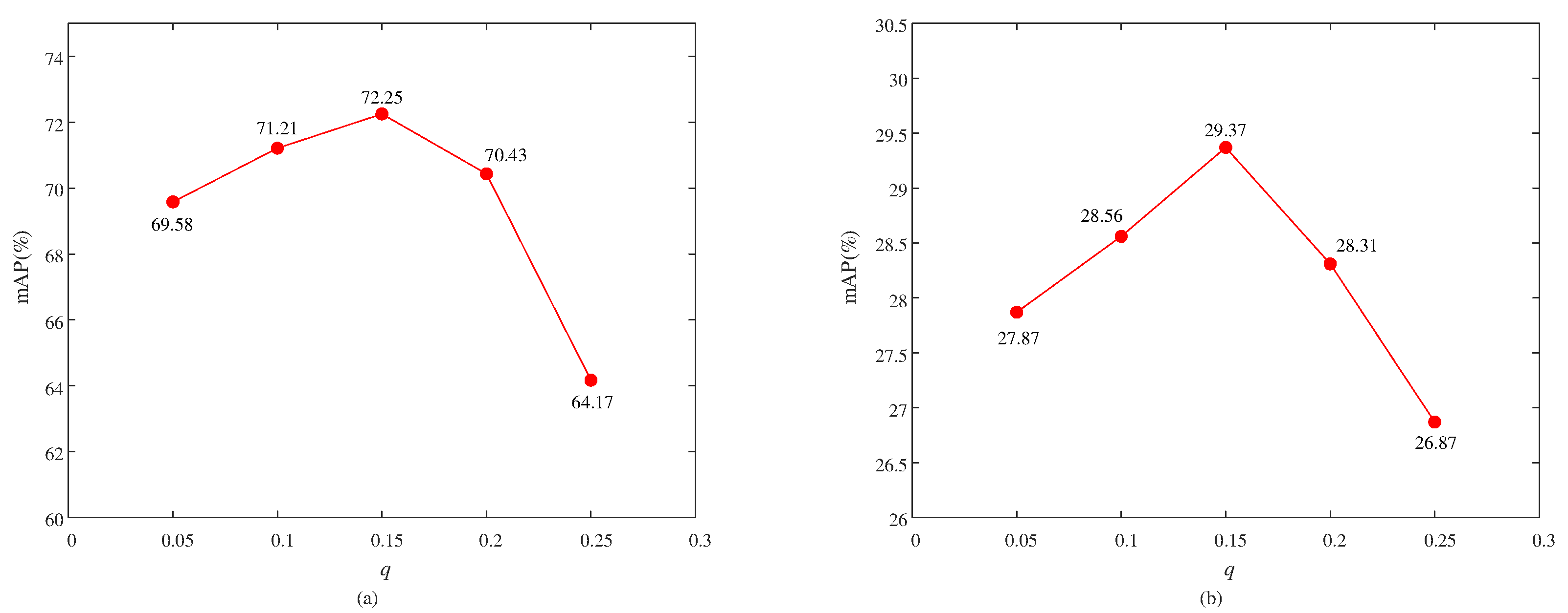
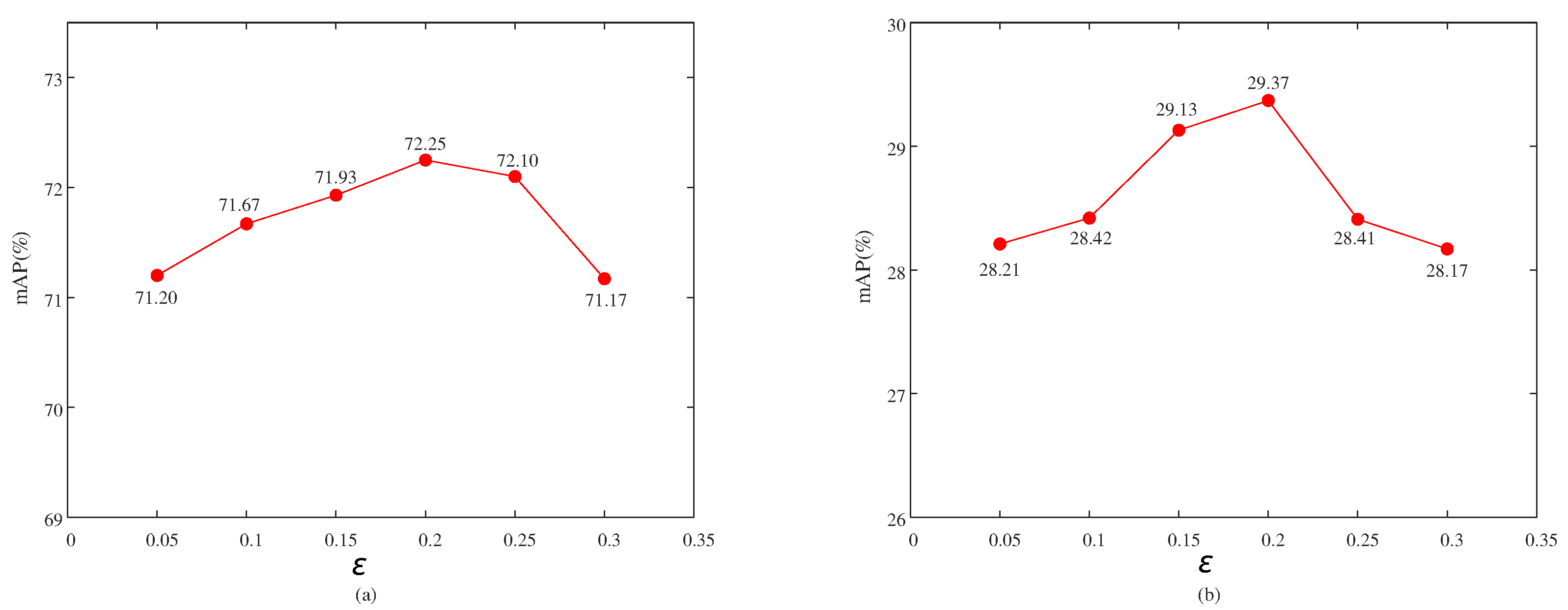
4.3. Parameter Analysis

(1) Parameter Analysis of q: The proportion q is a crucial hyperparameter controlling the selection of initial seed instances. Its effect is quantitatively evaluated on the DIOR and NWPU VHR-10.v2 datasets in terms of mAP. To analyze its impact, we conduct experiments by varying q among {0.05, 0.10, 0.15, 0.20, 0.25}. As shown in Figure 2, the model achieves the highest mAP when q = 0.15. Therefore, q is set to 0.15.

(2) Parameter Analysis of ε: As illustrated in Figure 3, the temperature parameter $\epsilon$ is quantitatively analyzed on the DIOR and NWPU VHR-10.v2 datasets in terms of mAP. Specifically, we evaluate $\epsilon$ over the range {0.05, 0.10, 0.15, 0.20, 0.25, 0.30} to assess its impact. The results show that both datasets achieve the highest mAP when $\epsilon$ = 0.2. Therefore, we set $\epsilon$ = 0.2 as the default value in our model.

(3) Parameter Analysis of δ: As illustrated in Figure 4, the $\delta$ is quantitatively analyzed in terms of mAP across the DIOR and NWPU VHR-10.v2 datasets. We evaluate $\delta$ over the range {50, 100, 150, 200} to assess its impact. The results show that both datasets achieve the highest mAP when $\delta$ = 100. Therefore, we set $\delta$ = 100 as the default value in our model.

4.4. Ablation Study

4.4.1. Quantitative Ablation Study

To validate the effectiveness of the FGSIM strategy, TAF loss, and their combination, we conduct an ablation study on the NWPU VHR-10.v2 dataset by incrementally integrating these components into the baseline model and evaluating their performance in terms of mAP and CorLoc.

We first examine the impact of the FGSIM strategy by comparing the baseline model with its variant incorporating FGSIM, denoted as Baseline + FGSIM in

Table 2. Ablation Study of FGSIM and TAF loss on the NWPU VHR-10.v2 dataset.

Baseline	FGSIM	TAF	NWPU VHR-10.v2
			mAP	CorLoc
✓			49.0	61.5
✓	✓		65.3	73.5
✓		✓	61.7	72.9
✓	✓	✓	72.5	78.6

. On the NWPU VHR-10.v2 dataset, Baseline + FGSIM achieves improvements of 16.3% in mAP and 12.0% in CorLoc, confirming the effectiveness of the FGSIM strategy.

Next, we assess the contribution of TAF loss by comparing the baseline model with Baseline + TAF (i.e., the combination of the baseline model and TAF loss). As shown in Table 2, Baseline + TAF achieves an improvement of 12.7% in mAP and 11.4% in CorLoc on the NWPU VHR-10.v2 dataset, demonstrating the effectiveness of TAF loss.

Finally, to analyze the combined effect of FGSIM and TAF loss, we compare the baseline model with Baseline + FGSIM + TAF on the NWPU VHR-10.v2 dataset. Baseline + FGSIM + TAF improves mAP by 23.5% and CorLoc by 17.1%, demonstrating the effectiveness of integrating FGSIM and TAF loss.

4.4.2. Subjective Ablation Study

We qualitatively compare the detection results of the baseline model with those of its enhanced variants (i.e., Baseline + FGSIM and Baseline + TAF) on the NWPU VHR-10.v2 dataset to further demonstrate the impact of the FGSIM strategy and TAF loss.

As shown in Figure 5, the Baseline fails to detect all airplanes with arbitrary orientations; however, our model can correctly identify them, which is attributed to the incorporation of the FGSIM module. The FGSIM module leverages feature similarity measurements to discover additional seed instances with lower class scores, thereby encouraging the model to detect as many foreground objects as possible.

As shown in Figure 6, the airplane on the right side of the image receives a high classification score but suffers from poor localization in the baseline model, indicating an inconsistency between classification confidence and localization accuracy. After applying the TAF loss, our model not only assigns a more accurate bounding box to the same airplane, but also provides a higher and more consistent classification score. This demonstrates that TAF loss effectively improves the consistency between classification and localization.

4.5. Quantitative Comparison with Popular Methods

To assess our model’s effectiveness, we conduct quantitative evaluations on the DIOR and NWPU VHR-10.v2 datasets in terms of CorLoc and mAP. Specifically, we compare its performance against two classical fully supervised object detection approaches (Faster R-CNN [49] and Fast R-CNN [34]) along with fifteen advanced WSOD models including WSDDN [15], MIST [24], OICR [16], DCL [9], CDN [22], SGPM [23], PILM [38], HQIM [36], the triple context-aware (TCA) model [19], the progressive contextual instance refinement (PCIR) model [18], the multiple instance graph (MIG) model [39], the self-guided proposal generation (SPG) model [37], the self-supervised adversarial and equivariant (SAE) network [50], instance-level feature refinement (ILFR) model [51], and multi-instance mining with dynamic localization (MIDL) model [52]. Among these, CDN and MIDL are rotation-invariant WSOD approaches.

As presented in

Table 3. Comparisons of different works in terms of mAP (%) on the NWPU VHR-10.v2 dataset.

Method	Airplane	Ship	Storage Tank	Baseball Diamond	Tennis Court	Basketball Court	Ground Track Field	Harbor	Bridge	Vehicle	mAP
Fast R-CNN [34]	90.9	90.6	89.3	47.3	100.0	85.9	84.9	88.2	80.3	69.8	82.7
Faster R-CNN [49]	90.9	86.3	90.5	98.2	89.7	69.6	100.0	80.1	61.5	78.1	84.5
WSDDN [15]	30.1	41.7	35.0	88.9	12.9	23.9	99.4	13.9	1.9	3.6	35.1
OICR [16]	13.7	67.4	57.2	55.2	13.6	39.7	92.8	0.2	1.8	3.7	34.5
MIST [24]	69.7	49.2	48.6	80.9	27.1	79.9	91.3	47.0	8.3	13.4	51.5
DCL [9]	72.7	74.3	37.1	82.6	36.9	42.3	84.0	39.6	16.8	35.0	52.1
PCIR [18]	90.8	78.8	36.4	90.8	22.6	52.2	88.5	42.4	11.7	35.5	55.0
MIG [39]	88.7	71.6	75.2	94.2	37.5	47.7	100.0	27.3	8.3	9.1	56.0
TCA [19]	89.4	78.2	78.4	90.8	35.3	50.4	90.9	42.4	4.1	28.3	58.8
CDN [22]	82.9	79.0	46.1	90.9	35.8	77.6	100.0	45.4	2.2	21.3	58.1
SAE [50]	82.9	74.5	50.2	96.7	55.7	72.9	100.0	36.5	6.3	31.9	60.7
SPG [37]	90.4	81.0	59.5	92.3	35.6	51.4	99.9	58.7	17.0	43.0	62.8
PILM [38]	87.6	81.0	57.3	94.0	36.4	80.4	100.0	56.9	9.8	35.6	63.8
SGPM [23]	90.7	79.9	69.3	97.5	41.6	77.5	100.0	44.4	17.2	33.5	65.2
HQIM [36]	90.8	80.5	73.4	96.6	47.4	78.9	100.0	43.9	18.4	33.5	66.2
ILFR [51]	90.8	81.6	56.6	91.7	51.9	69.5	100.0	53.4	16.3	40.5	65.2
MIDL [52]	90.1	65.3	67.4	90.9	50.2	62.8	99.8	33.2	16.7	42.3	61.9
Ours	90.8	81.4	72.9	94.7	56.4	81.8	100.0	68.7	15.3	62.7	72.5

, our model achieves 72.5% mAP on the NWPU VHR-10.v2 dataset, surpassing WSDDN by 37.4%, OICR by 38.0%, MIST by 21.0%, DCL by 20.4%, PCIR by 17.5%, MIG by 16.5%, TCA by 13.7%, CDN by 14.4%, SAE by 11.8%, SPG by 9.7%, PILM by 8.7%, SGPM by 7.3%, HQIM by 6.3%, ILFA by 7.3%, and MIDL by 10.6%, respectively. Similarly, as shown in

Table 4. Comparisons of different works in terms of CorLoc (%) on the NWPU VHR-10.v2 dataset.

Method	Airplane	Ship	Storage Tank	Baseball Diamond	Tennis Court	Basketball Court	Ground Track Field	Harbor	Bridge	Vehicle	CorLoc
WSDDN [15]	22.3	36.8	40.0	92.5	18.0	24.2	99.3	14.8	1.7	2.9	35.2
OICR [16]	29.4	83.3	20.5	81.8	40.9	32.1	86.6	7.4	3.7	14.4	40.0
MIST [24]	90.2	82.5	80.3	98.6	48.5	87.4	98.3	66.5	14.6	35.8	70.3
DCL [9]	-	-	-	-	-	-	-	-	-	-	69.7
PCIR [18]	100.0	93.1	64.1	99.3	64.8	79.3	89.7	63.0	13.3	52.2	71.9
MIG [39]	97.8	90.3	87.2	98.7	54.9	64.2	100.0	74.1	13.0	21.6	70.2
TCA [19]	96.9	91.8	95.1	88.7	66.9	62.8	96.0	54.2	19.6	55.5	72.8
CDN [22]	96.5	81.3	67.1	95.3	66.9	86.3	100.0	74.2	10.3	46.5	72.4
SAE [50]	97.1	91.7	87.8	98.7	40.9	81.1	100.0	70.4	14.8	52.2	73.5
SPG [37]	98.1	92.7	70.1	99.7	51.9	80.1	96.2	72.4	13.0	60.0	73.4
PILM [38]	94.4	86.6	68.5	97.8	69.8	87.5	100.0	68.6	16.0	56.6	74.3
SGPM [23]	98.2	93.8	89.3	99.1	50.2	88.9	100.0	71.0	12.3	51.2	75.4
HQIM [36]	99.3	94.8	91.7	98.0	58.4	91.7	100.0	68.8	13.6	56.7	76.9
ILFR [51]	98.6	94.7	76.4	83.9	61.3	82.4	100.0	78.1	19.5	57.2	75.2
Ours	92.1	92.9	87.2	94.1	68.4	90.7	100.0	78.9	18.9	62.7	78.6

, our model attains 76.89% CorLoc on the same dataset, demonstrating improvements of 43.4%, 38.6%, 8.3%, 8.9%, 6.7%, 8.4%, 5.8%, 6.2%, 5.1%, 5.2%, 4.3%, 3.2%, 1.7%, and 3.4% over WSDDN, OICR, MIST, DCL, PCIR, MIG, TCA, CDN, SAE, SPG, PILM, SGPM, HQIM, and ILFR, respectively.

As presented in

Table 5. Comparisons of different works in terms of mAP (%) on the DIOR dataset.

Method	Airplane	Airport	Baseball Field	Basketball Court	Bridge	Chimney	Dam	Expressway Service Area	Expressway Toll Station	Golf Field
Fast R-CNN [34]	44.2	66.8	67.0	60.5	15.6	72.3	52.0	65.9	44.8	72.1
Faster R-CNN [49]	50.3	62.6	66.0	80.9	28.8	68.2	47.3	58.5	48.1	60.4
WSDDN [15]	9.1	39.7	37.8	20.2	0.3	12.3	0.6	0.7	11.9	4.9
OICR [16]	8.7	28.3	44.1	18.2	1.3	20.2	0.1	0.7	29.9	13.8
MIST [24]	32.0	39.9	62.7	29.0	7.5	12.9	0.3	5.1	17.4	51.0
DCL [9]	20.9	22.7	54.2	11.5	6.0	61.0	0.1	1.1	31.0	30.9
PCIR [18]	30.4	36.1	54.2	26.6	9.1	58.6	0.2	9.7	36.2	32.6
MIG [39]	22.2	52.6	62.8	25.8	8.5	67.4	0.7	8.9	28.7	57.3
TCA [19]	25.1	30.8	62.9	40.0	4.1	67.8	8.1	23.8	29.9	22.3
CND [22]	31.1	15.8	10.7	54.5	15.7	33.9	3.7	12.3	37.2	12.0
SAE [50]	20.6	62.4	62.7	23.5	7.6	64.6	0.2	34.5	30.6	55.4
SPG [37]	31.3	36.7	62.8	29.1	6.1	62.7	0.3	15.0	30.1	35.0
PILM [38]	29.1	49.8	70.9	41.4	7.2	45.5	0.2	35.4	36.8	60.8
SGLM [23]	39.1	64.6	64.4	26.9	6.3	62.3	0.9	12.2	26.3	55.3
HQIM [36]	42.2	65.0	66.2	25.7	6.7	60.2	1.3	13.5	25.3	57.8
ILFR [51]	32.9	70.5	63.2	45.7	0.2	69.7	0.2	12.4	39.4	56.4
MIDL [52]	38.1	12.3	62.9	27.4	10.7	62.0	0.1	0.6	32.2	49.4
Ours	37.5	62.7	60.9	30.2	9.2	63.4	1.9	16.8	37.6	54.7
Method	Ground track field	Harbor	Overpass	Ship	Stadium	Storage tank	Tennis court	Train station	Vehicle	Windmill	mAP
Fast R-CNN [34]	62.9	46.2	38.0	32.1	71.0	35.0	58.3	37.9	19.2	38.1	50.0
Faster R-CNN [34]	67.0	43.9	46.9	58.5	52.4	42.4	79.5	48.0	34.8	65.4	55.5
WSDDN [15]	42.5	4.7	1.1	0.7	63.0	4.0	6.1	0.5	4.6	1.1	13.3
OICR [16]	57.4	10.7	11.1	9.1	59.3	7.1	0.7	0.1	9.1	0.4	16.5
MIST [24]	49.5	5.4	12.2	29.4	35.5	25.4	0.8	4.6	22.2	0.8	22.2
DCL [9]	56.5	5.1	2.7	9.1	63.7	9.1	10.4	0.0	7.3	0.8	20.2
PCIR [18]	58.5	8.6	21.6	12.1	64.3	9.1	13.6	0.3	9.1	7.5	24.9
MIG [39]	47.7	23.8	0.8	6.4	54.1	13.2	4.1	14.8	0.2	2.4	25.1
TCA [19]	53.9	24.8	11.1	9.1	46.4	13.7	31.0	1.5	9.1	1.0	25.8
CDN [22]	44.2	60.9	0.7	12.3	37.2	37.5	19.2	52.6	1.1	2.9	26.7
SAE [50]	52.7	17.6	6.9	9.1	51.6	15.4	1.7	14.4	1.4	9.2	27.1
SPG [37]	48.0	27.1	12.0	10.0	60.0	15.1	21.0	9.9	3.2	0.1	25.8
PILM [38]	48.5	14.0	25.1	18.5	48.9	11.7	11.9	3.5	11.3	1.7	28.6
SGLM [23]	60.6	9.4	23.1	13.4	57.4	17.7	1.5	14.0	11.5	3.5	28.5
HQIM [36]	61.4	10.4	20.4	14.1	58.6	18.9	2.2	13.6	10.0	4.7	28.9
ILFR [51]	55.3	16.6	0.6	9.1	54.8	18.1	11.0	16.1	9.1	1.1	29.1
MIDL [52]	64.7	7.4	29.0	9.1	53.8	11.3	57.0	7.7	1.6	0.5	27.3
Our	57.9	23.7	24.9	17.2	55.9	11.3	12.1	14.9	12.8	3.6	30.5

, our model achieves 30.5% mAP on the challenging DIOR dataset, surpassing WSDDN, OICR, MIST, DCL, PCIR, MIG, TCA, CDN, SAE, SPG, PILM, SGPM, HQIM, ILFR, andMIDL by 17.2%, 14.0%, 8.3%, 10.3%, 5.6%, 5.4%, 4.7%, 3.8%, 3.4%, 4.7%, 1.9%, 2.0%, 1.6%, 1.4%, and 3.2%, respectively. Similarly, as shown in

Table 6. Comparisons of different works in terms of CorLoc (%) on the DIOR dataset.

Method	Airplane	Airport	Baseball Field	Basketball Court	Bridge	Chimney	Dam	Expressway Service Area	Expressway Toll Station	Golf Field
WSDDN [15]	5.7	59.9	94.2	55.9	4.9	23.4	1.0	6.8	44.5	12.8
OICR [16]	16.0	51.5	94.8	55.8	3.6	23.9	0.0	4.8	56.7	22.4
MIST [24]	91.6	53.2	93.5	66.3	10.8	30.7	1.5	14.3	35.2	47.5
DCL [9]	-	-	-	-	-	-	-	-	-	-
PCIR [18]	93.1	45.6	95.5	68.3	3.6	92.1	0.2	5.4	58.4	47.5
MIG [39]	77.0	46.9	95.4	63.6	23.0	95.1	0.2	17.0	57.9	50.8
TCA [19]	81.6	51.3	96.2	73.5	5.0	94.7	15.9	32.8	46.0	48.6
CDN [22]	85.6	58.7	95.6	95.6	10.5	96.2	0.5	17.6	60.7	45.9
SAE [50]	91.2	69.4	95.5	67.5	18.9	97.8	0.2	70.5	54.3	51.4
SPG [37]	80.5	32.0	98.7	65.0	15.2	96.1	22.5	17.0	46.1	51.0
PILM [38]	85.5	68.9	96.8	75.8	11.6	94.7	0.8	67.5	60.5	46.5
SGLM [23]	92.2	58.3	97.8	74.2	16.2	95.2	0.3	51.3	56.2	52.3
HQIM [36]	94.1	59.3	98.1	70.5	17.6	94.6	4.8	52.2	54.3	53.5
ILFR [51]	88.3	69.1	98.8	69.4	19.9	97.8	0.3	24.7	56.2	54.4
Ours	91.9	70.4	98.5	71.6	18.2	92.4	1.9	67.6	59.4	59.7
Method	Ground track field	Harbor	Overpass	Ship	Stadium	Storage tank	Tennis court	Train station	Vehicle	Windmill	CorLoc
WSDDN [15]	89.9	5.5	10.0	23.0	98.5	79.6	15.1	3.5	11.6	3.2	32.4
OICR [16]	91.4	18.2	18.7	31.8	98.3	81.3	7.5	1.2	15.8	2.0	34.8
MIST [24]	87.1	38.6	23.4	50.7	80.5	89.2	22.4	11.5	22.2	2.4	43.6
DCL [9]	-	-	-	-	-	-	-	-	-	-	42.2
PCIR [18]	88.6	15.8	5.2	39.5	98.1	85.6	13.4	56.5	9.7	0.6	46.1
MIG [39]	89.4	42.1	19.8	37.9	97.9	80.7	13.8	10.3	10.5	6.9	46.8
TCA [19]	85.3	38.9	20.2	30.6	84.6	91.5	56.3	3.8	10.5	1.3	48.4
CDN [22]	90.6	51.5	17.4	45.7	89.7	72.0	11.3	10.6	17.9	6.5	47.9
SAE [50]	88.3	48.0	2.3	33.6	14.1	83.4	65.6	19.9	16.4	2.9	49.4
SPG [37]	89.2	49.5	22.0	35.2	98.6	90.0	32.6	12.7	10.0	2.3	48.3
PILM [38]	75.2	50.5	28.3	39.7	92.6	77.0	55.1	10.1	20.9	5.6	53.2
SGLM [23]	91.7	48.6	23.0	32.7	98.8	89.3	43.5	19.5	18.3	4.0	53.2
HQIM [36]	93.0	49.7	22.0	34.8	99.0	90.4	44.1	18.3	17.5	10.5	53.9
ILFR [51]	89.6	49.1	19.4	34.5	96.7	84.7	63.2	15.6	11.6	3.4	52.3
Ours	91.1	52.1	23.7	44.7	98.7	86.9	45.2	20.9	18.7	8.7	56.1

, our model attains 56.1% CorLoc on the DIOR dataset, demonstrating improvements of 23.7%, 21.3%, 12.5%, 13.9%, 10.0%, 9.3%, 7.7%, 8.2%, 6.7%, 7.8%, 2.9%, 2.9%, 2.2%, and 3.8% over WSDDN, OICR, MIST, DCL, PCIR, MIG, TCA, CDN, SAE, SPG, PILM, SGPM, HQIM, and ILFR, respectively.

Furthermore, our approach narrows the performance gap between WSOD and fully supervised object detection models across both datasets. The results further confirm the effectiveness of our method, highlighting its advantage over advanced WSOD approaches on two datasets.

4.6. Subjective Evaluation

Figure 7 and Figure 8 illustrate our model’s detection results on the NWPU VHR-10.v2 and DIOR datasets, respectively. We visualize results from 24 test images to demonstrate the model’s effectiveness. Furthermore, to qualitatively compare our model with four representative WSOD approaches (i.e., OICR, MIST, PILM, and SGPM), we present detailed visual analyses in Figure 9. Specifically, as shown in Figure 9a, existing methods fail to detect all airplanes, especially those with arbitrary orientations. In contrast, our model accurately identifies all airplane instances. This improvement is due to two key components: First, the FGSIM strategy leverages feature similarity between instances to mine additional seed instances with lower class scores, thus providing richer supervisory signals. Second, the original RSI and its rotated counterpart are processed by separate ICR branches, allowing for consistent predictions via iterative supervision between ICR branches. In Figure 9b, methods such as MIST, PILM, and SGPM misclassify the shadows of storage tanks as foreground objects. Our model avoids this misclassification thanks to a contrastive loss that enforces intra-class feature similarity while enhancing inter-class distinction. Finally, in Figure 9c,d, other methods show inaccurate localization, with some boxes encompassing background or irrelevant regions. By contrast, our model assigns both accurate categories and precise locations to foreground instances, benefiting from the TAF loss.

4.7. Performance on Natural Images

To further evaluate the generalization capability of our method, we conduct comparisons with two fully supervised object detection methods and four WSOD methods on the PASCAL VOC 2007 dataset [53]. The PASCAL VOC 2007 dataset consists of 9963 images, divided into a training set (2501 images), a validation set (2510 images), and a test set. Following standard practice, we use both the training and validation sets for model training and evaluate performance on the test set. The training configuration for PASCAL VOC 2007 is similar to that of the NWPU VHR-10.v2 dataset.

As reported in

Table 7. Comparisons with popular models on the PASCAL VOC 2007 dataset in terms of mAP (%).

Method	Aeroplane	Bicycle	Bird	Boat	Bottle	Bus	Car	Cat	Chair	Cow
Fast R-CNN [34]	74.5	78.3	69.2	53.2	36.6	77.3	78.2	82.0	40.7	72.7
Faster R-CNN [49]	70.0	80.6	70.1	57.3	49.9	78.2	80.4	82.0	52.2	75.3
WSDDN [15]	39.4	50.1	31.5	16.3	12.6	64.5	42.8	42.6	10.1	35.7
OICR [16]	58.0	62.4	31.1	19.4	13.0	65.1	62.2	28.4	24.8	44.7
PCL [35]	54.4	69.0	39.3	19.2	15.7	62.9	64.4	30.0	25.1	52.5
MELM [54]	55.6	66.9	34.2	29.1	16.4	68.8	68.1	43.0	25.0	65.6
Ours	69.7	70.1	54.6	39.5	33.6	70.2	78.7	72.1	34.1	70.5
Method	Diningtable	Dog	Horse	Motorbike	Person	Pottedplant	Sheep	Sofa	Train	Tvmonitor	mAP
Fast R-CNN [34]	67.9	79.6	79.2	73.0	69.0	30.1	65.4	70.2	75.8	65.8	66.9
Faster R-CNN [49]	67.2	80.3	79.8	75.0	76.3	39.1	68.3	67.3	81.1	67.6	69.9
WSDDN [15]	24.9	38.2	34.4	55.6	9.4	14.7	30.2	40.7	54.7	46.9	34.8
OICR [16]	30.6	25.3	37.8	65.5	15.7	24.1	41.7	46.9	64.3	62.6	41.2
PCL [35]	44.4	19.6	39.3	67.7	17.8	22.9	46.6	57.5	58.6	63.0	43.5
MELM [54]	45.3	53.2	49.6	68.6	2.0	25.4	52.5	56.8	62.1	57.1	47.3
Ours	45.9	64.5	63.1	75.7	31.8	27.9	59.2	61.5	69.8	68.9	58.1

, our method achieves a mAP of 58.1% on the PASCAL VOC 2007 test set, outperforming WSDDN, OICR, PCL, and MELM by 23.3%, 16.9%, 14.6%, and 10.8%, respectively. Moreover, as illustrated in Figure 10, our model is able to accurately localize and classify foreground objects, demonstrating both high category precision and bounding box quality.

5. Discussion

In this work, we presented a novel approach to WSOD in RSIs, which addresses two key challenges prevalent in current WSOD models: the tendency to overlook less-obvious objects and the inconsistency between classification and regression tasks. We proposed an FGSIM strategy to effectively select reliable seed instances and a TAF loss to ensure the synchronization of classification and regression. In this section, we will discuss the effectiveness of these contributions and explore their implications.

One of the main challenges in WSOD for RSIs is the tendency of existing models to overlook less-obvious objects because they select the top-scoring proposals as seed instances. This limitation arises because the highest-scoring proposals may correspond to more prominent objects, while smaller, less obvious objects are often missed. Our proposed FGSIM strategy addresses this issue by first selecting multiple high-scoring proposals and then expanding this selection by mining lower-scoring but reliable proposals based on the feature similarities between samples. Furthermore, a contrastive loss is introduced to establish a reliable feature similarity threshold for FGSIM by enforcing intra-class similarity and inter-class distinctiveness. Our experimental results demonstrate the efficacy of the FGSIM strategy in overcoming this challenge. By utilizing both high-scoring and feature-similar low-scoring proposals, our model successfully detects objects that would have otherwise been missed by traditional WSOD models.

Another challenge faced by existing WSOD models is the inconsistency between the classification and regression branches. Many models use separate losses for classification and regression, but these losses are typically optimized independently, which can lead to suboptimal performance. To address this, we introduced the TAF loss, which dynamically adjusts the weights of the classification and regression losses based on the localization and classification difficulty scores. By aligning the two tasks, the TAF loss encourages the model to learn both classification and localization jointly, thus improving overall performance. Our experimental results validate the effectiveness of the TAF loss. The synchronized optimization of classification and regression enables our model to achieve better localization accuracy without sacrificing classification performance.

6. Conclusions

This paper proposes FGSIM, a feature-guided seed instance mining strategy designed to address the challenge where current models often detect only salient objects while overlooking less-obvious ones due to their reliance on selecting the highest-scoring proposal as the seed instance. FGSIM first selects high-scoring proposals as initial seed instances and then expands this set based on a feature similarity measure between samples. To establish a reliable similarity threshold for FGSIM, a contrastive loss is introduced to encourage consistent feature representations within the same category. In addition, we propose a TAF loss to address inconsistencies between the classification and regression branches. The TAF loss leverages classification and localization difficulty scores as weights for the regression and classification losses, respectively, enabling their joint optimization. Additionally, the original RSI and its rotated counterpart are fed into different ICR branches, facilitating consistent predictions for detected instances before and after rotation through supervision between neighboring ICR branches. Ablation studies demonstrate the effectiveness of each component, while comparisons with popular models on two RSI benchmarks verify the overall superiority of our approach.

The proposed method has significant implications for improving WSOD in RSIs, especially in cluttered or complex scenes where conventional methods struggle with non-salient targets. However, the localization accuracy remains dependent on the quality of initial proposals, which are generated using traditional selective search algorithms that may not align well with object boundaries. Future work aims to explore more advanced, segmentation-driven, or learning-based proposal generation mechanisms to obtain high-quality proposals, further improving localization precision.

References

1. Șerban, R.D.; Șerban, M.; He, R.; Jin, H.; Li, Y.; Li, X.; Wang, X.; Li, G. 46-Year (1973–2019) Permafrost Landscape Changes in the Hola Basin, Northeast China Using Machine Learning and Object-Oriented Classification. Remote Sens. 2021, 13, 910. [Google Scholar] [CrossRef]
2. Li, W.; Yu, Y.; Meng, F.; Duan, J.; Zhang, X. A image fusion and U-Net approach to improving crop planting structure multi-category classification in irrigated area. J. Intell. Fuzzy Syst. 2023, 45, 185–198. [Google Scholar] [CrossRef]
3. Chen, Q.; Huang, M.; Wang, H. A Feature Discretization Method for Classification of High-Resolution Remote Sensing Images in Coastal Areas. IEEE Trans. Geosci. Remote Sens. 2021, 59, 8584–8598. [Google Scholar] [CrossRef]
4. Maneepong, K.; Yamanotera, R.; Akiyama, Y.; Miyazaki, H.; Miyazawa, S.; Akiyama, C.M. Towards High-Resolution Population Mapping: Leveraging Open Data, Remote Sensing, and AI for Geospatial Analysis in Developing Country Cities—A Case Study of Bangkok. Remote Sens. 2025, 17, 1204. [Google Scholar] [CrossRef]
5. Somanath, S.; Naserentin, V.; Eleftheriou, O.; Sjölie, D.; Wästberg, B.S.; Logg, A. Towards Urban Digital Twins: A Workflow for Procedural Visualization Using Geospatial Data. Remote Sens. 2024, 16, 1939. [Google Scholar] [CrossRef]
6. Tian, T.; Pan, M.; Zhang, F.; Cong, W.; Han, X.; Zhang, J. A 3D GIS-based underground construction deformation display system. In Proceedings of the 2010 18th International Conference on Geoinformatics, Beijing, China, 18–20 June 2010; pp. 1–6. [Google Scholar] [CrossRef]
7. Zeng, B.; Gao, S.; Xu, Y.; Zhang, Z.; Li, F.; Wang, C. Detection of Military Targets on Ground and Sea by UAVs with Low-Altitude Oblique Perspective. Remote Sens. 2024, 16, 1288. [Google Scholar] [CrossRef]
8. Qian, X.; Lin, C.; Chen, Z.; Wang, W. SAM-Induced Pseudo Fully Supervised Learning for Weakly Supervised Object Detection in Remote Sensing Images. Remote Sens. 2024, 16, 1532. [Google Scholar] [CrossRef]
9. Yao, X.; Feng, X.; Han, J.; Cheng, G.; Guo, L. Automatic weakly supervised object detection from high spatial resolution remote sensing images via dynamic curriculum learning. IEEE Trans. Geosci. Remote Sens. 2020, 59, 675–685. [Google Scholar] [CrossRef]
10. Fasana, C.; Pasini, S.; Milani, F.; Fraternali, P. Weakly Supervised Object Detection for Remote Sensing Images: A Survey. Remote Sens. 2022, 14, 5362. [Google Scholar] [CrossRef]
11. Qian, X.; Wu, B.; Cheng, G.; Yao, X.; Wang, W.; Han, J. Building a Bridge of Bounding Box Regression Between Oriented and Horizontal Object Detection in Remote Sensing Images. IEEE Trans. Geosci. Remote Sens. 2023, 61, 5605209. [Google Scholar] [CrossRef]
12. Shi, W.; Zhang, S.; Zhang, S. CAW-YOLO: Cross-Layer Fusion and Weighted Receptive Field-Based YOLO for Small Object Detection in Remote Sensing. CMES-Comput. Model. Eng. Sci. 2024, 139, 3209–3231. [Google Scholar] [CrossRef]
13. Zhou, S.; Liu, Z.; Luo, H.; Qi, G.; Liu, Y.; Zuo, H.; Zhang, J.; Wei, Y. GCA2Net: Global-Consolidation and Angle-Adaptive Network for Oriented Object Detection in Aerial Imagery. Remote Sens. 2025, 17, 1077. [Google Scholar] [CrossRef]
14. Shi, R.; Zhang, L.; Wang, G.; Jia, S.; Zhang, N.; Wang, C. GD-Det: Low-Data Object Detection in Foggy Scenarios for Unmanned Aerial Vehicle Imagery Using Re-Parameterization and Cross-Scale Gather-and-Distribute Mechanisms. Remote Sens. 2025, 17, 783. [Google Scholar] [CrossRef]
15. Bilen, H.; Vedaldi, A. Weakly supervised deep detection networks. In Proceedings of the 2016 IEEE Conference on Computer Vision and Pattern Recognition, Las Vegas, NV, USA, 27–30 June 2016; pp. 2846–2854. [Google Scholar]
16. Tang, P.; Wang, X.; Bai, X.; Liu, W. Multiple instance detection network with online instance classifier refinement. In Proceedings of the 2017 IEEE Conference on Computer Vision and Pattern Recognition, Honolulu, HI, USA, 21–26 July 2017; pp. 2843–2851. [Google Scholar]
17. Huang, Z.; Zou, Y.; Kumar, B.V.K.V.; Huang, D. Comprehensive Attention Self-Distillation for Weakly-Supervised Object Detection. In Proceedings of the Advances in Neural Information Processing Systems; Larochelle, H., Ranzato, M., Hadsell, R., Balcan, M., Lin, H., Eds.; Curran Associates, Inc.: Newry, UK, 2020; Volume 33, pp. 16797–16807. [Google Scholar]
18. Feng, X.; Han, J.; Yao, X.; Cheng, G. Progressive contextual instance refinement for weakly supervised object detection in remote sensing images. IEEE Trans. Geosci. Remote Sens. 2020, 58, 8002–8012. [Google Scholar] [CrossRef]
19. Feng, X.; Han, J.; Yao, X.; Cheng, G. TCANet: Triple Context-Aware Network for Weakly Supervised Object Detection in Remote Sensing Images. IEEE Trans. Geosci. Remote Sens. 2021, 59, 6946–6955. [Google Scholar] [CrossRef]
20. Feng, X.; Yao, X.; Cheng, G.; Han, J. Weakly Supervised Rotation-Invariant Aerial Object Detection Network. In Proceedings of the 2022 IEEE/CVF Conference on Computer Vision and Pattern Recognition (CVPR), New Orleans, LA, USA, 18–24 June 2022; pp. 14126–14135. [Google Scholar] [CrossRef]
21. Wu, Z.; Wen, J.; Xu, Y.; Yang, J.; Zhang, D. Multiple Instance Detection Networks With Adaptive Instance Refinement. IEEE Trans. Multimed. 2023, 25, 267–279. [Google Scholar] [CrossRef]
22. Huo, Y.; Qian, X.; Li, C.; Wang, W. Multiple Instance Complementary Detection and Difficulty Evaluation for Weakly Supervised Object Detection in Remote Sensing Images. IEEE Geosci. Remote Sens. Lett. 2023, 20, 6006505. [Google Scholar] [CrossRef]
23. Qian, X.; Li, C.; Wang, W.; Yao, X.; Cheng, G. Semantic segmentation guided pseudo label mining and instance re-detection for weakly supervised object detection in remote sensing images. Int. J. Appl. Earth Obs. Geoinf. 2023, 119, 103301. [Google Scholar] [CrossRef]
24. Ren, Z.; Yu, Z.; Yang, X.; Liu, M.Y.; Lee, Y.J.; Schwing, A.G.; Kautz, J. Instance-aware, context-focused, and memory-efficient weakly supervised object detection. In Proceedings of the IEEE/CVF Conference on Computer Vision and Pattern Recognition, Seattle, WA, USA, 14–19 June 2020; pp. 10598–10607. [Google Scholar]
25. Qian, X.; Wang, C.; Li, C.; Li, Z.; Zeng, L.; Wang, W.; Wu, Q. Multiscale Image Splitting Based Feature Enhancement and Instance Difficulty Aware Training for Weakly Supervised Object Detection in Remote Sensing Images. IEEE J. Sel. Top. Appl. Earth Obs. Remote Sens. 2023, 16, 7497–7506. [Google Scholar] [CrossRef]
26. Seo, J.; Bae, W.; Sutherland, D.J.; Noh, J.; Kim, D. Object Discovery via Contrastive Learning for Weakly Supervised Object Detection. In Proceedings of the Computer Vision—ECCV 2022—17th European Conference, Tel Aviv, Israel, 23–27 October 2022; pp. 312–329. [Google Scholar]
27. Qian, X.; Wang, C.; Wang, W.; Yao, X.; Cheng, G. Complete and Invariant Instance Classifier Refinement for Weakly Supervised Object Detection in Remote Sensing Images. IEEE Trans. Geosci. Remote Sens. 2024, 62, 5627713. [Google Scholar] [CrossRef]
28. Chang, S.; Deng, Y.; Zhang, Y.; Zhao, Q.; Wang, R.; Zhang, K. An Advanced Scheme for Range Ambiguity Suppression of Spaceborne SAR Based on Blind Source Separation. IEEE Trans. Geosci. Remote Sens. 2022, 60, 5230112. [Google Scholar] [CrossRef]
29. Qian, X.; Huo, Y.; Cheng, G.; Yao, X.; Li, K.; Ren, H.; Wang, W. Incorporating the Completeness and Difficulty of Proposals Into Weakly Supervised Object Detection in Remote Sensing Images. IEEE J. Sel. Top. Appl. Earth Obs. Remote Sens. 2022, 15, 1902–1911. [Google Scholar] [CrossRef]
30. Uijlings, J.R.; Van De Sande, K.E.; Gevers, T.; Smeulders, A.W. Selective search for object recognition. Int. J. Comput. Vis. 2013, 104, 154–171. [Google Scholar] [CrossRef]
31. Liu, B.; Gao, Y.; Guo, N.; Ye, X.; Wan, F.; You, H.; Fan, D. Utilizing the Instability in Weakly Supervised Object Detection. In Proceedings of the IEEE/CVF Conference on Computer Vision and Pattern Recognition (CVPR) Workshops, Long Beach, CA, USA, 15–20 June 2019. [Google Scholar]
32. Chen, Z.; Fu, Z.; Jiang, R.; Chen, Y.; Hua, X.S. SLV: Spatial Likelihood Voting for Weakly Supervised Object Detection. In Proceedings of the IEEE/CVF Conference on Computer Vision and Pattern Recognition (CVPR), Seattle, WA, USA, 14–19 June 2020. [Google Scholar]
33. Feng, X.; Yao, X.; Shen, H.; Cheng, G.; Xiao, B.; Han, J. Learning an Invariant and Equivariant Network for Weakly Supervised Object Detection. IEEE Trans. Pattern Anal. Mach. Intell. 2023, 45, 11977–11992. [Google Scholar] [CrossRef]
34. Girshick, R. Fast r-cnn. In Proceedings of the IEEE International Conference on Computer Vision, Santiago, Chile, 7–13 December 2015; pp. 1440–1448. [Google Scholar]
35. Tang, P.; Wang, X.; Bai, S.; Shen, W.; Bai, X.; Liu, W.; Yuille, A. PCL: Proposal Cluster Learning for Weakly Supervised Object Detection. IEEE Trans. Pattern Anal. Mach. Intell. 2020, 42, 176–191. [Google Scholar] [CrossRef]
36. Xing, P.; Huang, M.; Wang, C.; Cao, Y. High-Quality Instance Mining and Weight Re-Assigning for Weakly Supervised Object Detection in Remote Sensing Images. Electronics 2024, 13, 4753. [Google Scholar] [CrossRef]
37. Cheng, G.; Xie, X.; Chen, W.; Feng, X.; Yao, X.; Han, J. Self-Guided Proposal Generation for Weakly Supervised Object Detection. IEEE Trans. Geosci. Remote Sens. 2022, 60, 5625311. [Google Scholar] [CrossRef]
38. Qian, X.; Huo, Y.; Cheng, G.; Gao, C.; Yao, X.; Wang, W. Mining High-Quality Pseudoinstance Soft Labels for Weakly Supervised Object Detection in Remote Sensing Images. IEEE Trans. Geosci. Remote Sens. 2023, 61, 5607615. [Google Scholar] [CrossRef]
39. Wang, B.; Zhao, Y.; Li, X. Multiple instance graph learning for weakly supervised remote sensing object detection. IEEE Trans. Geosci. Remote Sens. 2021, 60, 5613112. [Google Scholar] [CrossRef]
40. Hosang, J.; Benenson, R.; Schiele, B. Learning non-maximum suppression. In Proceedings of the IEEE Conference on Computer Vision and Pattern Recognition, Honolulu, HI, USA, 21–26 July 2017; pp. 4507–4515. [Google Scholar]
41. Khosla, P.; Teterwak, P.; Wang, C.; Sarna, A.; Tian, Y.; Isola, P.; Maschinot, A.; Liu, C.; Krishnan, D. Supervised Contrastive Learning. arXiv 2021, arXiv:2004.11362. [Google Scholar]
42. Lin, T.Y.; Goyal, P.; Girshick, R.; He, K.; Dollár, P. Focal Loss for Dense Object Detection. In Proceedings of the 2017 IEEE International Conference on Computer Vision (ICCV), Venice, Italy, 22–29 October 2017; pp. 2999–3007. [Google Scholar] [CrossRef]
43. Cheng, G.; Zhou, P.; Han, J. Learning Rotation-Invariant Convolutional Neural Networks for Object Detection in VHR Optical Remote Sensing Images. IEEE Trans. Geosci. Remote Sens. 2016, 54, 7405–7415. [Google Scholar] [CrossRef]
44. Li, K.; Cheng, G.; Bu, S.; You, X. Rotation-Insensitive and Context-Augmented Object Detection in Remote Sensing Images. IEEE Trans. Geosci. Remote Sens. 2018, 56, 2337–2348. [Google Scholar] [CrossRef]
45. Li, K.; Wan, G.; Cheng, G.; Meng, L.; Han, J. Object detection in optical remote sensing images: A survey and a new benchmark. ISPRS J. Photogramm. Remote Sens. 2020, 159, 296–307. [Google Scholar] [CrossRef]
46. Deselaers, T.; Alexe, B.; Ferrari, V. Weakly supervised localization and learning with generic knowledge. Int. J. Comput. Vis. 2012, 100, 275–293. [Google Scholar] [CrossRef]
47. Simonyan, K.; Zisserman, A. Very deep convolutional networks for large-scale image recognition. arXiv 2014, arXiv:1409.1556. [Google Scholar]
48. Krizhevsky, A.; Sutskever, I.; Hinton, G.E. ImageNet Classification with Deep Convolutional Neural Networks. In Proceedings of the Conference Advances in Neural Information Processing Systems, Lake Tahoe, NV, USA, 3–6 December 2012; pp. 1097–1105. [Google Scholar]
49. Ren, S.; He, K.; Girshick, R.; Sun, J. Faster R-CNN: Towards real-time object detection with region proposal networks. IEEE Trans. Pattern Anal. Mach. Intell. 2016, 39, 1137–1149. [Google Scholar] [CrossRef]
50. Feng, X.; Yao, X.; Cheng, G.; Han, J.; Han, J. SAENet: Self-Supervised Adversarial and Equivariant Network for Weakly Supervised Object Detection in Remote Sensing Images. IEEE Trans. Geosci. Remote Sens. 2022, 60, 5610411. [Google Scholar] [CrossRef]
51. Zheng, S.; Wu, Z.; Xu, Y.; Wei, Z. Weakly Supervised Object Detection for Remote Sensing Images via Progressive Image-Level and Instance-Level Feature Refinement. Remote Sens. 2024, 16, 1203. [Google Scholar] [CrossRef]
52. Guo, C.; Ma, Z.; Zhao, Y.; Cao, C.; Jiang, Z.; Zhang, H. Multi-instance mining with dynamic localization for weakly supervised object detection in remote-sensing images. Int. J. Remote Sens. 2025, 46, 3487–3512. [Google Scholar] [CrossRef]
53. Everingham, M.; Van Gool, L.; Williams, C.K.; Winn, J.; Zisserman, A. The pascal visual object classes (voc) challenge. Int. J. Comput. Vis. 2010, 88, 303–338. [Google Scholar] [CrossRef]
54. Wan, F.; Wei, P.; Jiao, J.; Han, Z.; Ye, Q. Min-entropy latent model for weakly supervised object detection. In Proceedings of the IEEE Conference on Computer Vision and Pattern Recognition, Salt Lake City, UT, USA, 18–22 June 2018; pp. 1297–1306. [Google Scholar]
Figure 1. The framework of our model.
Remotesensing 17 01673 g001
Figure 2. Parameter analysis of q on the NWPU VHR-10.v2 (a) and DIOR (b) datasets.
Remotesensing 17 01673 g002
Figure 3. Parameter analysis of ε on the NWPU VHR-10.v2 (a) and DIOR (b) datasets.
Remotesensing 17 01673 g003
Figure 4. Parameter analysis of δ on the NWPU VHR-10.v2 (a) and DIOR (b) datasets.
Remotesensing 17 01673 g004
Figure 5. Qualitative comparison of detection results between the Baseline and Baseline + FGSIM on the NWPU VHR-10.v2 dataset.
Remotesensing 17 01673 g005
Figure 6. Qualitative comparison of detection results between the Baseline and Baseline + TAF loss on the NWPU VHR-10.v2 dataset.
Remotesensing 17 01673 g006
Figure 7. Detection results of our model on the NWPU VHR-10.v2 dataset.
Remotesensing 17 01673 g007
Figure 8. Detection results of our model on the DIOR dataset.
Remotesensing 17 01673 g008
Figure 9. Qualitative comparison of detection results between our model and advanced WSOD models on two RSI benchmarks. (a,d) are sampled from the NWPU VHR-10.v2 dataset, while (b,c) are from the DIOR dataset.
Remotesensing 17 01673 g009
Figure 10. Detection results of our model on the PASCAL VOC 2007 dataset.
Remotesensing 17 01673 g010