


Automated Eddy Identification and Tracking in the Northwest Pacific Based on Conventional Altimeter and SWOT Data


Abstract
1. Introduction
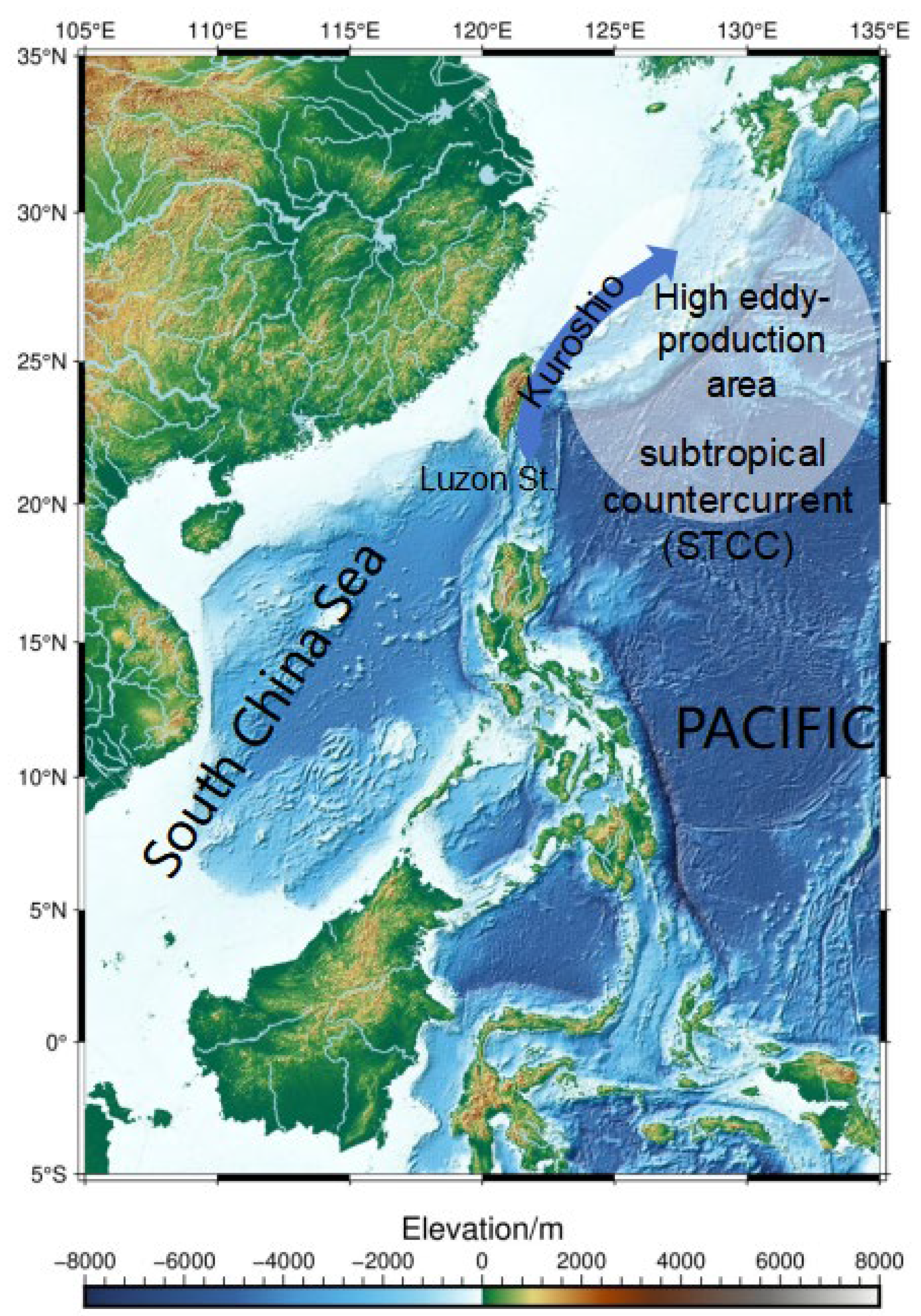
2. Study Area
3. Satellite Altimeter and In Situ Data
3.1. Altimeter Data
3.2. Drifter Data
4. Methods for Automatic Identification and Tracking of Eddies
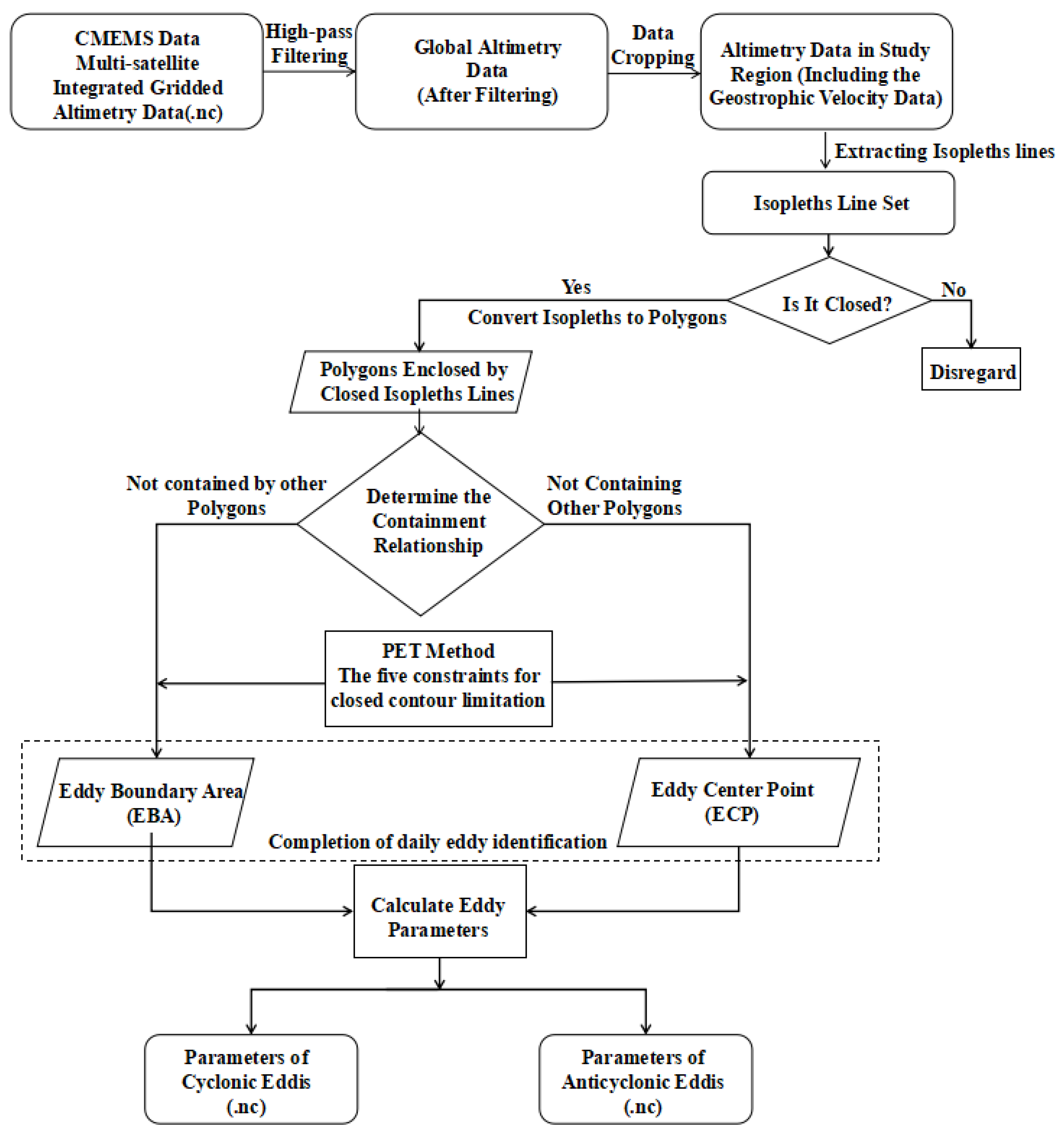
4.1. Automated Identification and Tracking
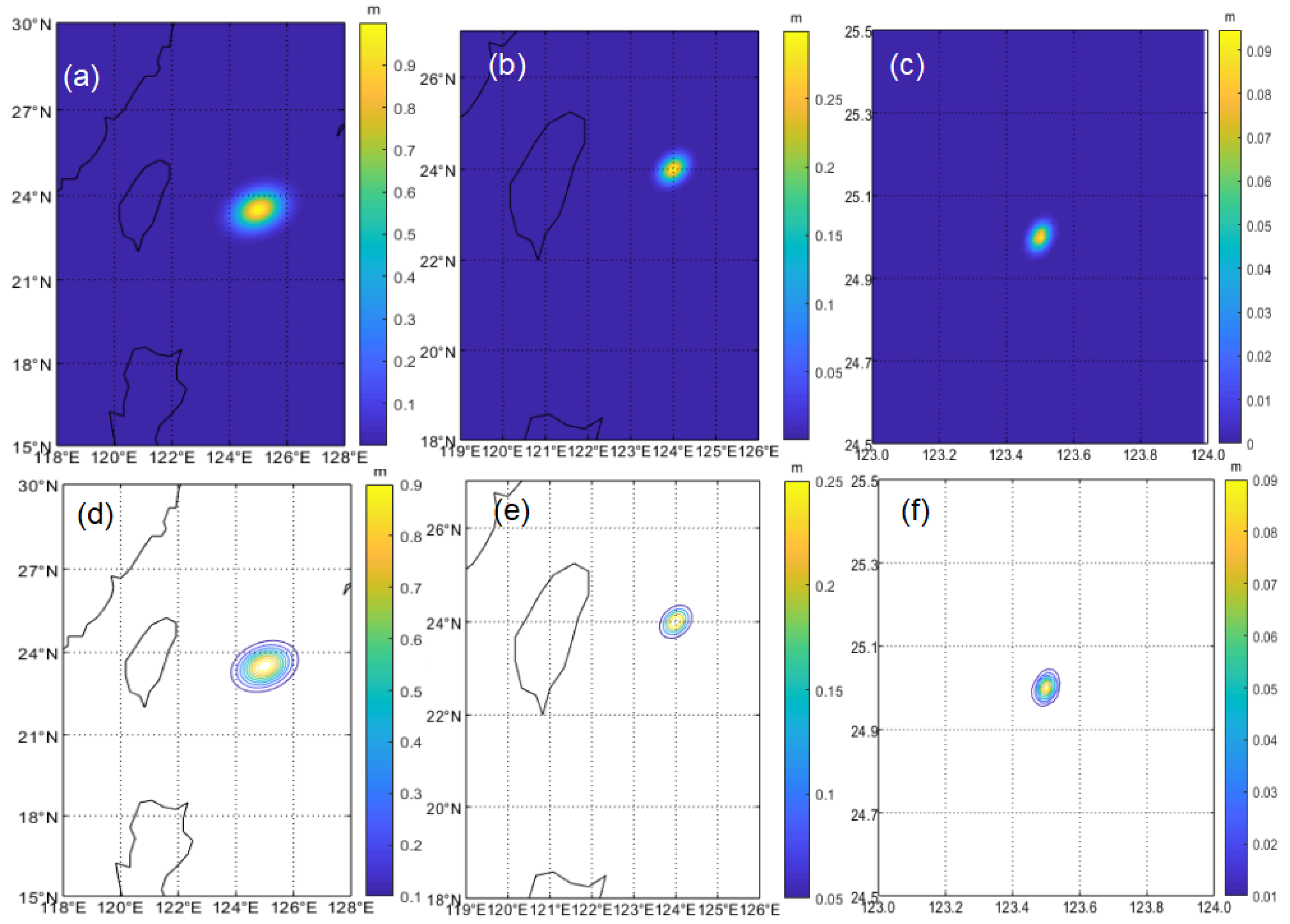
4.2. Validating PET Identification Using Simulated Eddies at Various Scales
5. Results and Discussions
5.1. Eddies from Conventional Altimeter Data
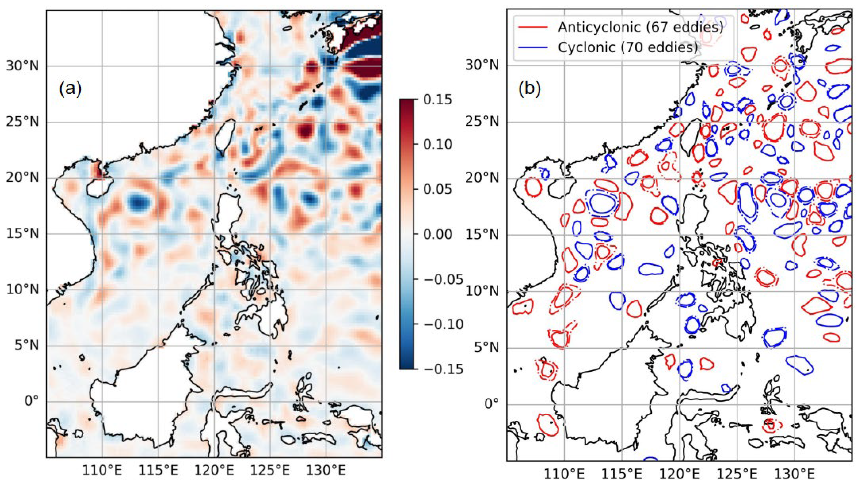
5.1.1. Snapshot of Ocean Eddies: A Case Study from 1 May 2023
5.1.2. Long-Term Spatiotemporal Characteristics of the Detected Eddies
5.1.3. Eddy Validation Using SVP Drifters
5.2. A Preliminary Assessment of SWOT Observations for Eddy Detection
5.2.1. ‘Eddy’ Detection Using Observations from SWOT’s One-Day Orbit
5.2.2. Eddy Detection Using Observations from SWOT’s 21-Day Orbit
6. Discussion
6.1. Errors Induced by High-Pass Filter
6.2. Limitations of PET in Identifying Submesoscale Eddies
7. Conclusions
Author Contributions
Funding
Data Availability Statement
Acknowledgments
Conflicts of Interest
Appendix A. Five Constraints for Closed Polygons
- An eddy’s closed contour includes only one eddy center SLA extremum, with anticyclonic eddies containing only one SLA maximum value and cyclonic eddies containing only one SLA minimum value, differing from the constraint of [1].
- The area of the region enclosed by the closed SLA isopleth lines is between 8 pixels and 1000 pixels. For submesoscale eddies, which are generally smaller than 10 km in radius, an excessive number of pixels may fail to accurately capture their compact structure and can lead to an overestimation of their ER during detection. Therefore, we set the maximum pixel value to 150 pixels.
- The eddy amplitude (Amplitude, A) is between 1 cm and 150 cm. A = |SLA_center—SLA_contour|, where SLA_center is the SLA at the center of the eddy within the closed SLA isopleth, and SLA_contour is the average SLA on that closed isopleth.
- For anticyclonic eddies, the formed eddy area only includes those pixels where the SLA value is greater than the current set SLA interval value; for cyclonic eddies, the formed eddy area only includes those pixels where the SLA value is less than the current set SLA interval value, with the interval value set at 0.4 cm in this study.
- Passing the shape test with Error_Shape ≤ 70%, where Error_Shape = Area_deviation/Area_(p_eff), with Area_(p_eff) being the area of the green best-fit circle shown in Figure 3 and Figure 4, which has the same area as the red closed contour, and Area_deviation being the area enclosed outside the green best-fit circle and within the red closed contour.
Appendix B. Elliptical Gaussian Functions for Simulated Eddies
References
- Chelton, D.B.; Schlax, M.G.; Samelson, R.M. Global observations of nonlinear mesoscale eddies. Prog. Oceanogr. 2011, 91, 167–216. [Google Scholar] [CrossRef]
- Chelton, D.B.; Schlax, M.G.; Samelson, R.M.; de Szoeke, R.A. Global observations of large oceanic eddies. Geophys. Res. Lett. 2007, 34, L15606. [Google Scholar] [CrossRef]
- Garabato, A.C.N.; Yu, X.; Callies, J.; Barkan, R.; Polzin, K.L.; Frajka-Williams, E.E.; Griffies, S.M. Kinetic energy transfers between mesoscale and submesoscale motions in the open ocean’s upper layers. J. Phys. Oceanogr. 2022, 52, 75–97. [Google Scholar] [CrossRef]
- Thomas, L.N.; Tandon, A.; Mahadevan, A. Submesoscale processes and dynamics. Ocean Model. Eddying Regime 2008, 177, 17–38. [Google Scholar]
- McWilliam, J.C. Fluid dynamics at the margin of rotational control. Environ. Fluid Mech. 2008, 8, 441–449. [Google Scholar] [CrossRef]
- McWilliams, J.C. Submesoscale currents in the ocean. Proc. R. Soc. A Math. Phys. Eng. Sci. 2016, 472, 20160117. [Google Scholar] [CrossRef]
- Qiu, B. Seasonal eddy field modulation of the North Pacific Subtropical Countercurrent: TOPEX/Poseidon observations and theory. J. Phys. Oceanogr. 1999, 29, 2471–2486. [Google Scholar] [CrossRef]
- Moum, J.N.; Nash, J.D. Mixing measurements on an equatorial ocean mooring. J. Atmos. Oceanic Technol. 2009, 26, 317–336. [Google Scholar] [CrossRef]
- Stammer, D.; Ray, R.D.; Andersen, O.B.; Arbic, B.K.; Bosch, W.; Carrère, L.; Thomas, M. Accuracy assessment of global barotropic ocean tide models. Rev. Geophys. 2014, 52, 243–282. [Google Scholar] [CrossRef]
- Zhang, Z.; Wang, W.; Qiu, B. Oceanic mass transport by mesoscale eddies. Science 2014, 345, 322–324. [Google Scholar] [CrossRef]
- Dong, C.; McWilliams, J.C.; Liu, Y.; Chen, D. Global heat and salt transports by eddy movement. Nat. Commun. 2014, 5, 3294. [Google Scholar] [CrossRef] [PubMed]
- Mensah, V.; Jan, S.; Andres, M.; Chang, M.H. Response of the Kuroshio east of Taiwan to mesoscale eddies and upstream variations. J. Oceanogr. 2020, 76, 271–288. [Google Scholar] [CrossRef]
- Isern-Fontanet, J.; García-Ladona, E.; Font, J. Identification of marine eddies from altimetric maps. J. Atmos. Oceanic Technol. 2003, 20, 772–778. [Google Scholar] [CrossRef]
- Okubo, A. Horizontal dispersion of floatable particles in the vicinity of velocity singularities such as convergences. Deep Sea Res. Oceanogr. Abstr. 1970, 17, 445–454. [Google Scholar] [CrossRef]
- Weiss, J. The dynamics of entropy transfer in two-dimensional hydrodynamics. Phys. D Nonlinear Phenom. 1991, 48, 273–294. [Google Scholar] [CrossRef]
- Fu, L.L.; Chelton, D.B.; Le Traon, P.Y.; Morrow, R. Eddy dynamics from satellite altimetry. Oceanography 2010, 23, 14–25. [Google Scholar] [CrossRef]
- Morrow, R.; Birol, F.; Griffin, D.; Sudre, J. Divergent pathways of cyclonic and anticyclonic ocean eddies. Geophys. Res. Lett. 2004, 31, 24. [Google Scholar] [CrossRef]
- Chaigneau, S.; Gizolme, A.; Grados, C. Mesoscale eddies of Peru in altimeter records: Identification algorithms and eddy spatio-temporal patterns. Prog. Oceanogr. 2008, 79, 106–119. [Google Scholar] [CrossRef]
- Hwang, C.; Chen, S.A. Circulations and eddies over the South China Sea derived from TOPEX/Poseidon altimetry. J. Geophys. Res. Ocean. 2000, 105, 23943–23965. [Google Scholar] [CrossRef]
- Barabinot, Y.; Speich, S.; Carton, X. Defining mesoscale eddies boundaries from in-situ data and a theoretical framework. J. Geophys. Res. Ocean. 2024, 129, e2023JC020422. [Google Scholar] [CrossRef]
- Lapeyre, G.; Klein, P. Impact of the small-scale elongated filaments on the oceanic vertical pump. J. Mar. Res. 2006, 64, 835–851. [Google Scholar] [CrossRef]
- Hewitt, H.; Fox-Kemper, B.; Pearson, B. The small scales of the ocean may hold the key to surprises. Nat. Clim. Change 2022, 12, 496–499. [Google Scholar] [CrossRef]
- Qiu, B.; Chen, S.; Klein, P.; Sasaki, H.; Sasai, Y. Seasonal mesoscale and submesoscale eddy variability along the North Pacific Subtropical Countercurrent. J. Phys. Oceanogr. 2014, 44, 3079–3098. [Google Scholar] [CrossRef]
- Michael, D.; Fu, L.L.; Lettenmaier, D.P.; Alsdorf, D.E.; Rodriguez, E.; Esteban-Fernandez, D. The Surface Water and Ocean Topography Mission: Observing Terrestrial Surface Water and Oceanic Submesoscale Eddies. Proc. IEEE 2010, 98, 766–779. [Google Scholar]
- Zhang, Z.; Miao, M.; Qiu, B.; Tian, J.; Jing, Z.; Chen, G.; Chen, Z.; Zhao, W. Submesoscale eddies detected by SWOT and moored observations in the Northwestern Pacific. Geophys. Res. Lett. 2024, 51, e2024GL110000. [Google Scholar] [CrossRef]
- Mason, E.; Pascual, A.; McWilliams, J.C. A new sea surface height–based code for oceanic mesoscale eddy tracking. J. Atmos. Ocean. Technol. 2014, 31, 1181–1188. [Google Scholar] [CrossRef]
- Mason, E.; Pascual, A.; Gaube, P.; Ruiz, S.; Pelegrí, J.L.; Delepoulle, A. Subregional characterization of mesoscale eddies across the Brazil-Malvinas Confluence. J. Geophys. Res. Oceans 2017, 122, 3329–3357. [Google Scholar] [CrossRef]
- Pegliasco, C.; Delepoulle, A.; Mason, E.; Morrow, R.; Faugère, Y.; Dibarboure, G. META3.1exp: A new global mesoscale eddy trajectory atlas derived from altimetry. Earth Syst. Sci. Data 2022, 14, 1087–1107. [Google Scholar] [CrossRef]
- Fu, L.L.; Pavelsky, T.; Cretaux, J.F.; Morrow, R.; Farrar, J.T.; Vaze, P.; Dibarboure, G. The Surface Water and Ocean Topography Mission: A breakthrough in radar remote sensing of the ocean and land surface water. Geophys. Res. Lett. 2024, 51, e2023GL107652. [Google Scholar] [CrossRef]
- Metzger, E.J.; Hurlburt, H.E. The nondeterministic nature of Kuroshio penetration and eddy shedding in the South China Sea. J. Phys. Oceanogr. 2001, 31, 1712–1732. [Google Scholar] [CrossRef]
- Yuan, D.; Han, W.; Hu, D. Anti-cyclonic eddies northwest of Luzon in summer-fall observed by satellite altimeters. Geophys. Res. Lett. 2007, 34, L13610. [Google Scholar] [CrossRef]
- Chen, G.; Hou, Y.; Chu, X. Mesoscale eddies in the South China Sea: Mean properties, spatiotemporal variability, and impact on thermohaline structure. J. Geophys. Res. Ocean. 2011, 116, C06018. [Google Scholar] [CrossRef]
- Xiu, P.; Chai, F.; Shi, L.; Xue, H.; Chao, Y. A census of eddy activities in the South China Sea during 1993–2007. J. Geophys. Res. Oceans 2010, 115, C03012. [Google Scholar] [CrossRef]
- He, Y.; Xie, J.; Cai, S. Interannual variability of winter eddy patterns in the eastern South China Sea. Geophys. Res. Lett. 2016, 43, 5185–5193. [Google Scholar] [CrossRef]
- Yuan, D.; Han, W.; Hu, D. Surface Kuroshio path in the Luzon Strait area derived from satellite remote sensing data. J. Geophys. Res. Ocean. 2006, 111, C11007. [Google Scholar] [CrossRef]
- Caruso, M.J.; Gawarkiewicz, G.G.; Beardsley, R. Interannual variability of the Kuroshio intrusion in the South China Sea. J. Oceanogr. 2006, 62, 559–575. [Google Scholar] [CrossRef]
- Jan, S.; Mensah, V.; Andres, M.; Chang, M.H.; Yang, Y.J. Eddy-Kuroshio interactions: Local and remote effects. J. Geophys. Res. Ocean. 2017, 122, 9744–9764. [Google Scholar] [CrossRef]
- Jan, S.; Chern, C.S.; Wang, J.; Chiou, M.D. Generation and propagation of baroclinic tides modified by the Kuroshio in the Luzon Strait. J. Geophys. Res. Ocean. 2012, 117, C2. [Google Scholar] [CrossRef]
- Zhang, Y.; Zhang, Z.; Chen, D.; Qiu, B.; Wang, W. Strengthening of the Kuroshio current by intensifying tropical cyclones. Science 2020, 368, 988–993. [Google Scholar] [CrossRef]
- Ren, Q.; Yu, F.; Nan, F.; Li, Y.; Wang, J.; Liu, Y.; Chen, Z. Effects of mesoscale eddies on intraseasonal variability of intermediate water east of Taiwan. Sci. Rep. 2022, 12, 9182. [Google Scholar] [CrossRef]
- Gómez-Navarro, L.; Cosme, E.; Sommer, J.L.; Papadakis, N.; Pascual, A. Development of an image de-noising method in preparation for the Surface Water and Ocean Topography Satellite Mission. Remote Sens. 2020, 12, 734. [Google Scholar] [CrossRef]
- Tréboutte, A.; Carli, E.; Ballarotta, M.; Carpentier, B.; Faugère, Y.; Dibarboure, G. KaRIn noise reduction using a convolutional neural network for the SWOT Ocean Products. Remote Sens. 2023, 15, 2183. [Google Scholar] [CrossRef]
- Lumpkin, R.; Pazos, M. Measuring surface currents with Surface Velocity Program drifters: The instrument, its data, and some recent results. Lagrangian Anal. Predict. Coast. Ocean Dyn. 2007, 39, 67. [Google Scholar]
- Pegliasco, C.; Chaigneau, A.; Morrow, R. Main eddy vertical structures observed in the four major Eastern Boundary Upwelling Systems. J. Geophys. Res. Oceans 2015, 120, 6008–6033. [Google Scholar] [CrossRef]
- Wang, Z.; Li, Q.; Sun, L.; Li, S.; Yang, Y.; Liu, S. The most typical shape of oceanic mesoscale eddies from global satellite sea level observations. Front. Earth Sci. 2015, 9, 202–208. [Google Scholar] [CrossRef]
- Hwang, C.; Wu, C.R.; Kao, R. TOPEX/Poseidon observations of mesoscale eddies over the Subtropical Countercurrent: Kinematic characteristics of an anticyclonic eddy and a cyclonic eddy. J. Geophys. Res. Ocean. 2004, 109, C08013. [Google Scholar] [CrossRef]
- Qiu, B.; Lukas, R. Seasonal and interannual variability of the North Equatorial Current, the Mindanao Current, and the Kuroshio along the Pacific western boundary. J. Geophys. Res. Oceans 1996, 101, 12315–12330. [Google Scholar] [CrossRef]
- Ferrari, R.; Wunsch, C. The distribution of eddy kinetic and potential energies in the global ocean. Tellus A Dyn. Meteorol. Oceanogr. 2010, 62, 92–108. [Google Scholar] [CrossRef]
- Qiu, B.; Chen, S. Variability of the Kuroshio extension jet, recirculation gyre, and mesoscale eddies on decadal time scales. J. Phys. Oceanogr. 2005, 35, 2090–2103. [Google Scholar] [CrossRef]
- Kamenkovich, V.M.; Leonov, Y.P.; Nechaev, D.A.; Byrne, D.A.; Gordon, A.L. On the influence of bottom topography on the Agulhas eddy. J. Phys. Oceanogr. 1996, 26, 892–912. [Google Scholar] [CrossRef]
- Qiu, B. Encyclopedia of Ocean Sciences; Academic Press: Cambridge, MA, USA, 2001; pp. 1413–1426. [Google Scholar]
- Chelton, D.B.; Schlax, M.G. Global observations of oceanic Rossby Waves. Science 1996, 272, 234–238. [Google Scholar] [CrossRef]
- Zhang, Z.; Zhao, W.; Qiu, B.; Tian, J. Anticyclonic eddy sheddings from Kuroshio loop and the accompanying cyclonic eddy in the northeastern South China Sea. J. Phys. Oceanogr. 2017, 47, 1243–1259. [Google Scholar] [CrossRef]
- Shi, Y.; Liu, X.; Liu, T.; Chen, D. Characteristics of mesoscale eddies in the vicinity of the Kuroshio: Statistics from satellite altimeter observations and OFES model data. J. Mar. Sci. Eng. 2022, 10, 1975. [Google Scholar] [CrossRef]
- Kamenkovich, I.; Berloff, P.; Pedlosky, J. Role of eddy forcing in the dynamics of multiple zonal jets in a model of the North Atlantic. J. Phys. Oceanogr. 2009, 39, 1361–1379. [Google Scholar] [CrossRef]
- Lee, I.H.; Ko, D.S.; Wang, Y.H.; Centurioni, L.; Wang, D.P. The mesoscale eddies and Kuroshio transport in the western North Pacific east of Taiwan from 8-year (2003–2010) model reanalysis. Ocean Dyn. 2013, 63, 1027–1040. [Google Scholar] [CrossRef]
- Chow, C.H.; Shih, Y.Y.; Chien, Y.T.; Chen, J.Y.; Fan, N.; Wu, W.C.; Hung, C.C. The wind effect on biogeochemistry in eddy cores in the Northern South China Sea. Front. Mar. Sci. 2021, 8, 717576. [Google Scholar] [CrossRef]
- Chu, F.; Si, Z.; Yan, X.; Liu, Z.; Yu, J.; Pang, C. Physical structure and evolution of a cyclonic eddy in the Northern South China sea. Deep Sea Res. Part I Oceanogr. Res. Pap. 2022, 189, 103876. [Google Scholar] [CrossRef]
- Simanungkalit, Y.A.; Pranowo, W.; Purba, N.; Riyantini, I.; Nurrahman, Y. Influence of El Nino Southern Oscillation (ENSO) phenomena on eddies variability in the northwest Pacific Ocean. IOP Conf. Ser. Earth Environ. Sci. 2018, 176, 012002. [Google Scholar] [CrossRef]
- Cheng, X.; Qi, Y. Variations of eddy kinetic energy in the South China Sea. J. Oceanogr. 2010, 66, 85–94. [Google Scholar] [CrossRef]
- Zhao, H.; Yue, X.; Wang, L.; Wu, X.; Chen, Z. Submesoscale short-lived eddies in the southwestern Taiwan Strait observed by high-frequency surface-wave radars. Remote Sens. 2024, 16, 589. [Google Scholar] [CrossRef]
- Yin, Y.; Lin, X.; Hou, Y. Seasonality of the Kuroshio intensity east of Taiwan modulated by mesoscale eddies. J. Mar. Syst. 2019, 193, 84–93. [Google Scholar] [CrossRef]
- Jia, F.; Wu, L.; Qiu, B. Seasonal modulation of eddy kinetic energy and its formation mechanism in the southeast Indian Ocean. J. Phys. Oceanogr. 2011, 41, 657–665. [Google Scholar] [CrossRef]
- Qiu, B.; Chen, S. Eddy-mean flow interaction in the decadally-modulating Kuroshio Extension system. Deep Sea Res. II 2010, 57, 1098–1110. [Google Scholar] [CrossRef]
- Yang, S.; Xing, J.; Sheng, J.; Chen, S.; Chen, D. A process study of interactions between a warm eddy and the Kuroshio Current in Luzon Strait: The fate of eddies. J. Mar. Syst. 2019, 194, 66–80. [Google Scholar] [CrossRef]
- Chen, C.T.A.; Jan, S.; Huang, T.H.; Tseng, Y.H. Spring of no Kuroshio intrusion in the southern Taiwan Strait. J. Geophys. Res. Ocean. 2010, 115, C8. [Google Scholar] [CrossRef]
- Fu, L.L.; Ferrari, R. Observing oceanic submesoscale processes from space. Eos 2008, 89, 488. [Google Scholar] [CrossRef]
- Tom, F.; d’Ovidio, F.; Gerald, D. Ocean Finescale Dynamics—SWOT Science Team Meeting 2024. Available online: https://swot.jpl.nasa.gov/events/63/2024-swot-science-team-meeting/ (accessed on 5 May 2025).
- Lévy, M.; Franks, P.J.S.; Smith, K.S. The role of submesoscale currents in structuring marine ecosystems. Nat. Commun. 2018, 9, 4758. [Google Scholar] [CrossRef]
- Alpers, W.; Brandt, P.; Lazar, A.; Dagorne, D.; Sow, B.; Faye, S.; Hansen, M.W.; Rubino, A.; Poulain, P.M.; Brehmer, P. A small-scale oceanic eddy off the coast of West Africa studied by multi-sensor satellite and surface drifter data. Remote Sens. Environ. 2013, 129, 132–143. [Google Scholar] [CrossRef]
- Karimova, S. Spiral eddies in the Baltic, Black and Caspian seas as seen by satellite radar data. Adv. Space Res. 2012, 50, 1107–1124. [Google Scholar] [CrossRef]
- Whalen, C.B.; De Lavergne, C.; Naveira Garabato, A.C.; Klymak, J.M.; MacKinnon, J.A.; Sheen, K.L. Internal wave-driven mixing: Governing processes and consequences for climate. Nat. Rev. Earth Environ. 2020, 1, 606–621. [Google Scholar] [CrossRef]
- Duo, Z.; Wang, W.; Wang, H. Oceanic mesoscale eddy detection method based on deep learning. Remote Sens. 2019, 11, 1921. [Google Scholar] [CrossRef]
- Sun, H.; Li, H.; Xu, M.; Yang, F.; Zhao, Q.; Li, C. A lightweight deep learning model for ocean eddy detection. Front. Mar. Sci. 2023, 10, 1266452. [Google Scholar] [CrossRef]
- Ioannou, A.; Guez, L.; Laxenaire, R.; Speich, S. Global Assessment of Mesoscale Eddies with TOEddies: Comparison Between Multiple Datasets and Colocation with In Situ Measurements. Remote Sens. 2024, 16, 4336. [Google Scholar] [CrossRef]
- Ni, Q.; Zhai, X.; Wilson, C.; Chen, C.; Chen, D. Submesoscale eddies in the South China Sea. Geophys. Res. Lett. 2021, 48, e2020GL091555. [Google Scholar] [CrossRef]


| Eddy Scale | Eddy Center | Semi-Major Axis (km) | Semi-Minor Axis (km) | Amplitude (m) | Rotation Angle |
|---|---|---|---|---|---|
| Large-scale eddy | (125°E, 23.5°N) | 125 | 93.75 | 1.0 | 30° |
| Mesoscale eddy | (124°E, 24°N) | 50 | 37.5 | 0.3 | 45° |
| Submesoscale eddy | (123.5°E, 25°N) | 5 | 3.75 | 0.1 | 60° |
| ER (km) | SR (km) | FCR (km) | Relative Errors Between ER and FCR | |
|---|---|---|---|---|
| Large-scale eddy | 113.89 | 50.63 | 108.25 | 5.2% |
| Mesoscale eddy | 47.73 | 27.57 | 43.30 | 10.2% |
| Submesoscale eddy | 6.02 | 6.02 | 4.33 | 39.0% |
Disclaimer/Publisher’s Note: The statements, opinions and data contained in all publications are solely those of the individual author(s) and contributor(s) and not of MDPI and/or the editor(s). MDPI and/or the editor(s) disclaim responsibility for any injury to people or property resulting from any ideas, methods, instructions or products referred to in the content. |
© 2025 by the authors. Licensee MDPI, Basel, Switzerland. This article is an open access article distributed under the terms and conditions of the Creative Commons Attribution (CC BY) license (https://creativecommons.org/licenses/by/4.0/).
Share and Cite
Zhang, L.; Hwang, C.; Liu, H.-Y.; Chang, E.T.Y.; Yu, D. Automated Eddy Identification and Tracking in the Northwest Pacific Based on Conventional Altimeter and SWOT Data. Remote Sens. 2025, 17, 1665. https://doi.org/10.3390/rs17101665
Zhang L, Hwang C, Liu H-Y, Chang ETY, Yu D. Automated Eddy Identification and Tracking in the Northwest Pacific Based on Conventional Altimeter and SWOT Data. Remote Sensing. 2025; 17(10):1665. https://doi.org/10.3390/rs17101665
Chicago/Turabian StyleZhang, Lan, Cheinway Hwang, Han-Yang Liu, Emmy T. Y. Chang, and Daocheng Yu. 2025. "Automated Eddy Identification and Tracking in the Northwest Pacific Based on Conventional Altimeter and SWOT Data" Remote Sensing 17, no. 10: 1665. https://doi.org/10.3390/rs17101665
APA StyleZhang, L., Hwang, C., Liu, H.-Y., Chang, E. T. Y., & Yu, D. (2025). Automated Eddy Identification and Tracking in the Northwest Pacific Based on Conventional Altimeter and SWOT Data. Remote Sensing, 17(10), 1665. https://doi.org/10.3390/rs17101665