A Comparative Evaluation of Two Bias Correction Approaches for SST Forecasting: Data Assimilation Versus Deep Learning Strategies

Abstract

This study introduces two distinct post-processing strategies to address systematic biases in sea surface temperature (SST) numerical forecasts, thereby enhancing SST predictive accuracy. The first strategy implements a spatiotemporal four-dimensional multi-grid analysis (4D-MGA) scheme within a three-dimensional variational (3D-Var) data assimilation framework. The second strategy establishes a hybrid deep learning architecture integrating empirical orthogonal function (EOF) analysis, empirical mode decomposition (EMD), and a backpropagation (BP) neural network (designated as EE–BP). The 4D-MGA strategy dynamically corrects systematic biases through a temporally coherent extrapolation of analysis increments, leveraging its inherent capability to characterize intrinsic temporal correlations in model error evolution. In contrast, the EE–BP strategy develops a bias correction model by learning the systematic biases of the SST numerical forecasts. Utilizing a satellite fusion SST dataset, this study conducted bias correction experiments that specifically addressed the daily SST numerical forecasts with 7-day lead times in the Kuroshio region south of Japan during 2017, systematically quantifying the respective error reduction potentials of both strategies. Quantitative verification reveals that EE–BP delivers enhanced predictive skill across all forecast horizons, achieving 18.1–22.7% root–mean–square error reduction compared to 1.2–9.1% attained by 4D-MGA. This demonstrates deep learning’s unique advantage in capturing nonlinear bias evolution patterns.

1. Introduction

Sea surface temperature (SST) plays a significant role in both climate and weather systems, as well as within ecosystems. The accurate prediction of SST provides a key source of information for various applications. Current SST forecasting methods primarily encompass three approaches: a numerical model, empirical statistics, and machine learning [1]. Numerical model methods simulate ocean dynamics by solving coupled hydrodynamic–thermodynamic equations to forecast SST [2]. Empirical statistical methods leverage historical data to build predictive relationships but often fail to resolve complex nonlinear processes [3]. Machine learning, particularly deep learning, offers advantages in capturing complex spatiotemporal patterns directly from the data [4]. As of now, SST forecasting remains predominantly reliant on numerical methods in the operational oceanography community. However, SST forecasts generated through numerical modeling frequently demonstrate systematic deviations, primarily stemming from three fundamental limitations: structural deficiencies inherent in computational frameworks, inadequately specified initial conditions, and errors in physical parameterization schemes [5]. Biases in SST forecasts can lead to significant inaccuracies in weather predictions, climate projections, and oceanographic studies. Therefore, bias correction is essential to improve the reliability and accuracy of SST numerical forecasts.

Statistical post-processing methods have become a mainstream solution for mitigating systematic errors in numerical weather prediction, primarily due to their operational affordability and demonstrated skill in refining forecast precision [6]. The emergence of machine learning techniques, however, is reshaping this paradigm by introducing data-driven post-processing frameworks capable of addressing inherent biases in both weather forecasts and climate projection models [7,8]. Researchers have also pioneered machine learning explorations for SST forecast bias correction in recent studies. For instance, Han et al. proposed a hybrid algorithm integrating empirical orthogonal function (EOF) analysis with a backpropagation (BP) neural network, achieving a 64% reduction in root–mean–square error (RMSE) for 1-day lead SST forecasts in the South China Sea [9]. Similarly, Fei et al. employed a convolutional long short-term memory (ConvLSTM) network enhanced with multi-attention mechanisms, reducing the RMSE for 1-day lead SST forecasts by 41% in the same region, but their approach overlooked the modulation effects of seasonal variations on bias characteristics [10]. For another sea area, Liu et al. utilized a LSTM neural network to decrease the mean absolute error of SST forecasts by 70%, yet their single-point training paradigm disregarded spatial correlations, necessitating point-wise modeling for regional applications and compromising computational efficiency [11]. Yuan et al. focused on global marine regions using a generative adversarial network (GAN)-based integrated model, which reduced forecast mean squared error (MSE) by 90.3% [12]. However, their monthly-averaged data framework is inadequate for operational rapid-response requirements. These studies reveal two limitations: (1) the existing methods mostly focus on bias correction for 1-day lead time forecasts, and there is a lack of research and discussion on the bias correction for multi-day continuous forecasts; (2) despite the achievements in the application of AI-based methods for SST bias correction, the requirements of bias correction in operational forecasting have not been considered. Additionally, the performance of neural network methods in handling different scales, such as interannual, seasonal, and daily scales, has not been systematically diagnosed.

In this study, we propose two distinct post-processing strategies to address systematic biases in SST numerical forecasts: (1) a data assimilation-based strategy implementing the spatiotemporal four-dimensional multi-grid analysis scheme, denoted as 4D-MGA [13], and (2) a hybrid deep learning-based strategy integrating EOF analysis, empirical mode decomposition (EMD), and a BP neural network, formally designated as EE–BP [14]. Specifically, the 4D-MGA framework is fundamentally grounded in a three-dimensional variational (3D-Var) assimilation scheme [15], with explicit temporal dimension integration. This spatiotemporal formulation establishes the methodology as a cost-effective post-processing mechanism for numerical forecast bias mitigation. It is worth noting that this critical distinction sets 4D-MGA apart from conventional data assimilation approaches, which are primarily designed for computationally expensive online bias correction systems [5]. By leveraging satellite fusion SST data, bias correction experiments are conducted targeting daily 7-day SST forecasts in 2017 in the Kuroshio region south of Japan, followed by systematic validation and comparative analysis to evaluate the efficacy of these two strategies.

The remainder of this paper is organized as follows. In Section 2, the data and methods used in this study are introduced. In Section 3, we present and analyze the results of the bias correction experiments. Finally, conclusions are given in Section 4.

2. Materials and Methods

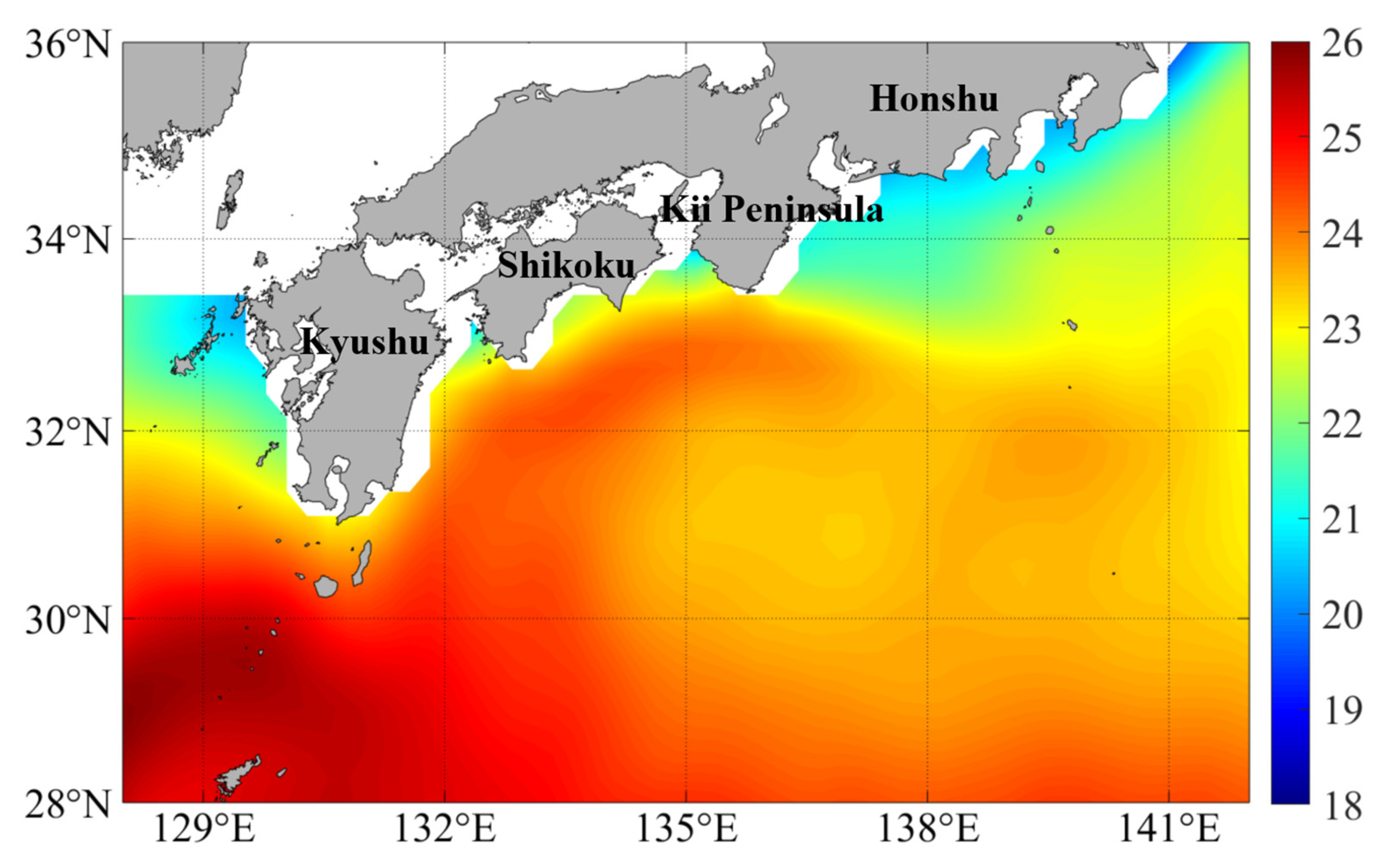
2.1. Data

This study comparatively evaluates these two novel post-processing strategies for bias correction in SST forecasts. The target area is the dynamically complex Kuroshio region in the south of Japan (28–36°N, 128–142°E; Figure 1). As the most powerful western boundary current in the North Pacific, the Kuroshio region exhibits strong nonlinear dynamics that generate pronounced SST variability through intense air–sea interactions [16,17]. This establishes the study area as an ideal validation testbed for assessing bias correction methodologies under challenging forecasting conditions.

The 7-day daily SST numerical forecasts used are generated by an ocean model custom-developed to simulate the 2017 Kuroshio large meander event [18]. The modeling framework utilizes the Princeton Ocean Model based on a generalized coordinate system (POMgcs) [19], driven by the ERA5 reanalysis data [20]. The initialization protocol employs a hybrid adaptive approach, synergistically integrating the ensemble adjustment Kalman filter with multi-grid variational analysis [21]. This ensures the effective assimilation of multi-source observations, including in situ temperature/salinity profiles, satellite-retrieved SSTs, and altimeter sea surface height anomalies. The configured model produced three-dimensional daily mean ocean state forecasts at 1/24° spatial resolution from 2016 to 2017, establishing a high-fidelity baseline for subsequent bias correction analysis.

For bias correction validation and performance evaluation, we employ the daily Optimum Interpolation SST (OISST, https://www.ncei.noaa.gov/products/optimum-interpolation-sst, accessed on 5 January 2025) v2.1 from the National Oceanic and Atmospheric Administration (NOAA) as the reference data [22]. The OISST dataset employs Advanced Very High-Resolution Radiometer (AVHRR) satellite data as its primary input, complemented by in situ measurements (ships, buoys, and Argo floats), with a horizontal resolution of 1/4° × 1/4°. Validation studies show that the RMSE of OISST in the Northwest Pacific is about 0.3–0.8 °C compared to independent buoy measurements [23].

Forecast biases are computed as the difference between the SST numerical forecasts and the OISST data. To ensure consistency in spatial resolution, the SST numerical forecasts are gridded to match the OISST grid resolution (1/4° × 1/4°) through spatial averaging.

2.2. Data Assimilation-Based Strategy for Bias Correction

The data assimilation-based strategy for bias correction leverages the temporal correlation property of 4D-MGA, which enables it to fit historical bias trends. By extrapolating the trends to the forecast period, the bias correction of the SST forecasts can be achieved.

2.2.1. Principle of 4D-MGA Method

The 4D-MGA method introduces the temporal and spatial correlations of the increments of the background fields due to the observations (called analysis increments) by incorporating the Laplace operator. The method employs a dichotomy-based multi-grid analysis (MGA) [24,25], enabling variational analysis from coarse to fine grids (from large scales to small scales). The 4D-MGA uses bilinear interpolation to calculate observation increments (biases). This interpolation scheme is applied to grids of different levels. On coarser grids, the interpolation spans larger spatial scales, capturing broad-scale error trends. On finer grids, the interpolation resolves localized biases with higher precision. This hierarchical mechanism ensures the robust spatiotemporal extrapolation of analysis increments. For the $n^{th}$ level of the grid, the number of nodes formed via dichotomy is $2^{(n-1)}+1$ for each individual dimension (3D spatial + 1D temporal), and the cost function for 4D-MGA is:

$$J^{\left(n\right)}\left({\tilde{\mathbf{X}}}^{\left(n\right)}\right)=\lambda {{\tilde{\mathbf{X}}}^{\left(n\right)}}^T{\mathbf{S}}^{\left(\mathrm{n}\right)}{\tilde{\mathbf{X}}}^{\left(n\right)}+{\displaystyle \frac{1}{2}}{\left[{\mathbf{H}}^{\left(n\right)}{\tilde{\mathbf{X}}}^{\left(n\right)}-{\tilde{\mathbf{Y}}}^{\left(n\right)}\right]}^T{{\mathbf{O}}^{\left(n\right)}}^{-1}\left[{\mathbf{H}}^{\left(n\right)}{\tilde{\mathbf{X}}}^{\left(n\right)}-{\tilde{\mathbf{Y}}}^{\left(n\right)}\right](n=1,\cdots N),$$

(1)

where $N$ is the last level of the grid; ${\tilde{\mathbf{X}}}^{\left(n\right)}$ is the analysis increment at the $n^{th}$ level, that is, the bias correction; ${\tilde{\mathbf{Y}}}^{\left(n\right)}$ is the increment of the observation relative to the background field (called observation increment) at the $n^{th}$ level; $\mathbf{H}$ denotes the linear interpolation operator from the background field to the observation point; $\mathbf{O}$ is the observation error covariance matrix; $\mathbf{S}$ denotes the Laplace operator; $\lambda {{\tilde{\mathbf{X}}}^{\left(n\right)}}^T{\mathbf{S}}^{\left(n\right)}{\tilde{\mathbf{X}}}^{\left(n\right)}$ is the smoothing term controlling the smoothing scale of the analysis field [25]; and $\lambda$ is the smoothing coefficient governing the weight of the smoothing term.

Equation (1) is solved iteratively by the minimization algorithm to obtain ${\tilde{\mathbf{X}}}^{\left(n\right)}$. The final results of 4D-MGA can be obtained by the superposition of the results from each level:

$${\mathbf{X}}^a={\mathbf{X}}^b+{\sum }_{n=1}^N{\tilde{\mathbf{X}}}^{\left(n\right)},$$

(2)

where ${\mathbf{X}}^a$ is the analysis results and ${\mathbf{X}}^b$ is the background field used in the analysis—in our case, the SST numerical forecasts of POMgcs.

We utilize the analysis increments of the analysis period (where observations are present) to extrapolate the bias trend via the smoothing term. For a one-dimensional grid with $M$ uniformly distributed grid points, the smoothing term can be described as:

$$\lambda {\tilde{\mathbf{X}}}^T\mathbf{S}\tilde{\mathbf{X}}=\lambda {\sum }_{i=2}^{M-1}{\left({\tilde{\mathbf{X}}}_{i-1}-2\cdot {\tilde{\mathbf{X}}}_i+{\tilde{\mathbf{X}}}_{i+1}\right)}^2.$$

(3)

Here, the Laplace operator serves to define the smoothness, or the spatiotemporal correlation of $\tilde{\mathbf{X}}$. When a grid point, such as ${\tilde{\mathbf{X}}}_i$, is adjusted under the influence of observations, all the other analysis increments will be constrained by the Laplace operator and adjusted following the variation trend of ${\tilde{\mathbf{X}}}_i$.

In this study, the 4D-MGA strategy employs the Laplace operator to enforce smoothness constraints, allowing for the linear extrapolation of bias trends from the analysis period (with observations) to the forecast period (without observations). During the analysis phase, increments are computed to minimize mismatches between forecasts and observations; these increments are then extended into the future under the assumption of gradual temporal evolution. Thereby, we can obtain the bias corrections for the forecast period.

2.2.2. Workflow of 4D-MGA

The spatiotemporal scale of MGA mainly depends on the smoothing coefficient and the space–time grid resolution. Through trial and error, the smoothing coefficient λ is set to 200. A large smoothing coefficient can better filter out the random errors and instantaneous signals in the analysis increments, thus retaining the large-scale temporal signals and enabling their effective extrapolation. In order to achieve better performance and lower computational cost, again, via trial-based calibration, the grid levels of the three dimensions used in this study are 7, 6, and 7 (longitude, latitude, and time dimensions), respectively. The finest grid comprises 65 × 33 × 65 nodes, with a horizontal resolution of 0.22° × 0.25° and a temporal grid step of 1 day.

The 4D-MGA primarily estimates bias by fitting temporal trends, including the following four steps:

• Background field generation: The background fields for each day within the time window (65 days) are set as ${\mathbf{X}}_1^b\cdots {\mathbf{X}}_{65}^b$. Taking the forecast start time (day 59) as the splitting point, days 1 to 58 are the analysis period, and days 59 to 65 are the forecast period. The background fields for the analysis period (${\mathbf{X}}_1^b\cdots {\mathbf{X}}_{58}^b$) are derived from the day 1 output of the 7-day SST forecasts, while the background fields for the forecast period (${\mathbf{X}}_{59}^b\cdots {\mathbf{X}}_{65}^b$) are the 7-day SST forecasts corresponding to ${\mathbf{X}}_{59}^b$.
• Observation increment calculation: For the analysis period, the observation increments (${\tilde{\mathbf{Y}}}_1\cdots {\tilde{\mathbf{Y}}}_{58}$) are calculated as the difference between the OISST data (${\mathbf{Y}}_1^{obs}\cdots {\mathbf{Y}}_{58}^{obs}$) and the background fields (${\mathbf{X}}_1^b\cdots {\mathbf{X}}_{58}^b$) for the corresponding dates. These observation increments are equal to the negative of the SST forecast biases.
• Data assimilation: Based on the smoothing term, 4D-MGA fits the observation increments (${\tilde{\mathbf{Y}}}_1\cdots {\tilde{\mathbf{Y}}}_{58}$) to generate smoothed analysis increments (${\tilde{\mathbf{X}}}_1\cdots {\tilde{\mathbf{X}}}_{58}$) for the forecast period, which are extrapolated to obtain the analysis increments (${\tilde{\mathbf{X}}}_{59}\cdots {\tilde{\mathbf{X}}}_{65}$) for the analysis period.
• Bias correction: Add the analysis increments (${\tilde{\mathbf{X}}}_{59}\cdots {\tilde{\mathbf{X}}}_{65}$) for the forecast period to the corresponding background fields (${\mathbf{X}}_{59}^b\cdots {\mathbf{X}}_{65}^b$), producing the bias-corrected SST analysis fields (${\mathbf{X}}_{59}^a\cdots {\mathbf{X}}_{65}^a$).

It is worth noting that the 4D-MGA bias correction strategy (the same as the following EE–BP strategy) is applied as a post-processing step to the SST numerical forecasts. Corrected outputs do not feed back into the subsequent forecast cycles, ensuring computational tractability and methodological isolation.

2.3. Deep Learning-Based Strategy for Bias Correction

The deep learning-based strategy (named EE–BP) constructs SST bias forecast models through learning systematic biases between the numerical model outputs and the OISST data. By integrating the spatiotemporal decomposition capability of EOF analysis, the multi-scale signal-processing capability of EMD, and the nonlinear learning capability of BP neural networks, the hybrid method becomes adept at capturing nonlinear signals (see Section 3).

2.3.1. Principle of EE–BP Method

The EOF analysis decomposes a data matrix into spatial modes (called EOFs) and their corresponding time series (called principal components, PCs) [26]. These EOFs and PCs capture the spatial distribution and temporal evolution characteristics of the data, respectively. The proportion of explained variance for each mode reflects the concentration of information, allowing for data simplification by selecting EOFs and PCs with high variance contributions. In this study, EOF analysis is applied to the SST forecast bias data. To balance information preservation and computational efficiency, we retain EOFs and PCs explaining 99.9% cumulative variance. This threshold is validated through comparative experiments. When the threshold rises, the increase in the correction effect diminishes, and the computational cost increases significantly. During the training of the bias correction model, the PCs are taken as the predicted values. With the predicted PCs, the SST biases can be reconstructed by combining them with the EOFs. The decomposition strategy reduces the computational complexity of neural network training by focusing on the temporal dimension. Compared with single-point neural network prediction, combining EOF analysis with the neural network improves the training efficiency while preserving the spatial correlations.

The EMD method is an effective signal-processing technique [27] that has been widely used in marine data processing and forecasting [28,29,30,31,32]. It adaptively decomposes complex and non-stationary signals into a series of intrinsic mode functions (IMFs) and a residual component. This decomposition smooths the signal and reduces its nonlinearity for further analysis. In this study, EMD is applied to each PC derived from EOF analysis, decomposing them into multiple IMFs. These IMFs represent different frequency components within the PCs, providing finer input features for neural network training. By trial and error, each PC is decomposed into three IMFs and one residual component, capturing the primary frequency components while avoiding over-decomposition and information redundancy.

The BP neural network, a multi-layer feedforward network trained via error backpropagation, excels in modeling nonlinear relationships through iterative weight optimization [4,33,34]. Its capability to approximate complex mappings between input–output variables proves advantageous for marine data characterized by strong nonlinearity, such as SST. Through extensive training, the BP network learns the weight relationships between input and output data, enabling accurate predictions even for new input data. Therefore, it is an ideal tool for bias correction and forecast accuracy improvement. In this study, we build three-layer (input–hidden–output) BP deep neural network models to conduct bias correction experiments for SST forecasts. The model performance is optimized by minimizing the RMSE between the predicted values and the ground truth values, using gradient descent. Predictions are generated through forward propagation, and weights are adjusted via backward error propagation to reduce errors iteratively. Additionally, the adaptive moment estimation (Adam) optimizer is employed to solve sparse gradients and noise problems. The rectified linear unit (ReLU) activation function is chosen to prevent the gradient vanishing problem and improve computational efficiency.

In this study, EOF analysis first decomposes the SST biases of the training set into EOFs and PCs, reducing dimensionality while preserving spatiotemporal correlations. EMD further decomposes each PC into multi-scale components (IMFs), isolating nonlinear and non-stationary signals. A BP neural network model is then trained on these IMFs. Leveraging the model, we can predict the future IMFs of the test set by inputting IMFs in the past few days. By reconstructing predicted IMFs into PCs and combining them with precomputed EOFs, EE–BP generates bias-corrected SST forecasts.

2.3.2. Workflow of EE–BP

The EE–BP combines EOF analysis, EMD analysis, and BP neural networks to build seven bias correction models for each forecast lead time. Figure 2 shows the flowchart of the EE–BP on day $m$ ($m=\mathrm{1,2}\cdots 7$), which includes the following five steps:

• EOF analysis: The 2016 SST forecast bias data are decomposed by EOF analysis to obtain EOFs and PCs. EOFs and PCs accounting for 99.90% of the cumulative variance are selected. The 2017 SST forecast bias data are projected onto the 2016 EOFs to derive the corresponding time series, called pseudo-PCs.
• EMD analysis: Each PC is decomposed into three IMFs and one residual component (called derived PCs) using EMD analysis. For each derived PC, the 2016 data are used as the training set, and the 2017 data are used as the test set.
• Model training: The BP neural network is constructed and trained on the training set. The size of the time window used to predict the derived PCs is set to $m$, which means that we use the preceding $m$-day-derived PC data to predict $m$-step-derived PCs.
• Model validation: based on the trained BP neural network, we predict the derived PCs in 2017, which are compared with the test set to evaluate model accuracy.
• Bias correction: The predicted derived PCs are reconstructed into PCs, which are then combined with EOFs to generate SST bias forecasts. By combining the biases and SST forecasts, the corrected SST can be obtained.

2.4. Evaluation Metrics

To evaluate the performance of the two bias correction strategies, we employ time-averaged and space-averaged bias, RMSE, and the spatial anomaly correlation coefficient (ACC) as the evaluation criteria. These calculation formulas are defined as follows:

$$bia{s}_i={\displaystyle \frac{1}{N}}{\sum }_{t=1}^N\left(x_{i,t}^P-x_{i,t}^T\right),$$

(4)

$$bia{s}_t={\displaystyle \frac{1}{M}}{\sum }_{i=1}^M\left(x_{i,t}^P-x_{i,t}^T\right),$$

(5)

$$RMS{E}_i={\displaystyle \frac{1}{N}}\sqrt{{\sum }_{t=1}^N{\left(x_{i,t}^P-x_{i,t}^T\right)}^2},$$

(6)

$$ACC={\displaystyle \frac{{\sum }_{i=1}^M\left(y_{i,t}^P-{\overline{y}}_t^P\right)\left(y_{i,t}^T-{\overline{y}}_t^T\right)}{\sqrt{{\sum }_{i=1}^M{\left(y_{i,t}^P-{\overline{y}}_t^P\right)}^2{\left(y_{i,t}^T-{\overline{y}}_t^T\right)}^2}}},$$

(7)

where $x_{i,t}^P$ and $x_{i,t}^T$ are the predictive and true SST of the $i^{th}$ grid point on the $t^{th}$ day, respectively; $M$ is the number of spatial grid points; and $N$ is the number of days of testing data. $Bia{s}_i$ is the mean error of the $i^{th}$ grid point and $bia{s}_t$ is the mean error on the $t^{th}$ day. Their joint use ensures a balanced evaluation of correction performance across temporal and spatial scales. $RMS{E}_i$ is the root–mean–square error of the $i^{th}$ grid point. $y_{i,t}^P=x_{i,t}^P-c_i$ and $y_{i,t}^T=x_{i,t}^T-c_i$ are the predictive and satellite SST anomalies (SSTA) of the $i^{th}$ grid point on the $t^{th}$ day, respectively; $c_i$ is the climatological SST of the OISST during from 1991 to 2020 of the $i^{th}$ grid point; and ${\overline{y}}_i^P={\displaystyle \frac{1}{M}}{y}_{i,t}^P$ and ${\overline{y}}_i^T={\displaystyle \frac{1}{M}}{y}_{i,t}^T$ are mean values of SSTA from prediction and satellite on the $t^{th}$ day, respectively. In this study, all evaluation metrics calculations use the OISST dataset as ground truth.

3. Results

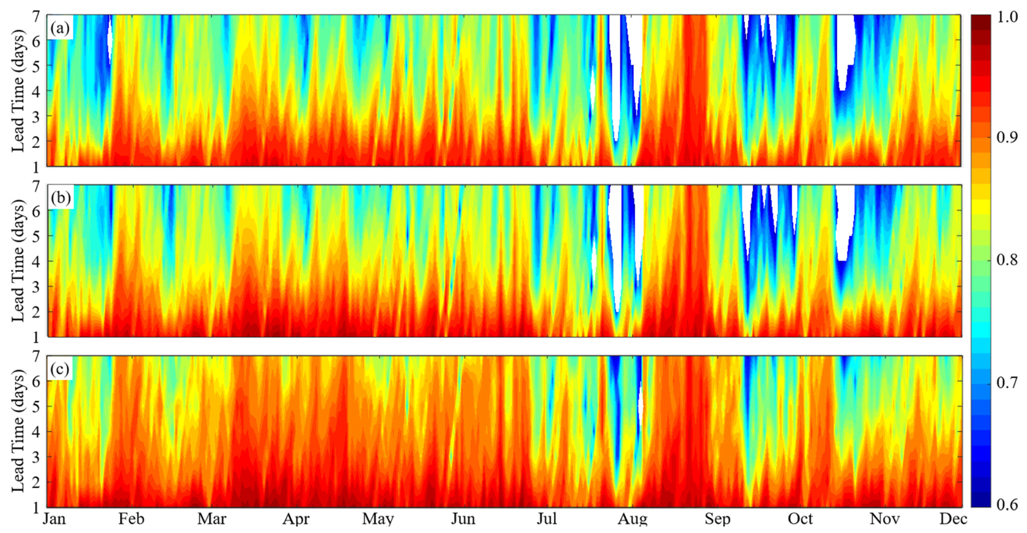
3.1. Overall Performance Evaluation

In this section, the SST forecast results in 2017 are analyzed to assess the overall performance of the two bias correction strategies (4D-MGA and EE–BP). Specifically, the means of RMSEs and spatial ACCs are calculated and compared in Figure 3. As shown in Figure 3b, the uncorrected 7-day forecasts exhibit ACC values consistently exceeding 0.6, confirming the reliability of the SST numerical forecasts [35]. Compared to the uncorrected forecasts (blue bars), both 4D-MGA (orange bars) and EE–BP (red bars) strategies demonstrate measurable improvements. 4D-MGA shows enhanced performance during days 1–3, reducing RMSEs by 4.5–9.1% while improving ACC values. However, its corrective effectiveness progressively declines with an increasing forecast horizon. In terms of RMSE, improvement in the forecast accuracy at day 7 is only 1.2%. Such results reflect the inherent defects of the 4D-MGA strategy—the bias correction of 4D-MGA is based on linear extrapolation. Therefore, the 4D-MGA strategy naturally lacks the capability to properly capture nonlinear signals. Moreover, to eliminate the random errors and instantaneous signals in the analysis increments, 4D-MGA has to employ a relatively large smoothing coefficient. This also leads to the fact that 4D-MGA is unable to capture the complex changes in temporal trends, which is also reflected in the discussion about the seasonal biases after correction in Section 3.2.3. Consequently, its performance in the aspect of bias correction for a long lead time is unsatisfactory. In contrast, the EE–BP maintains stable corrective performance across all seven forecast lead times. After bias correction by the EE–BP, the RMSEs decrease from 0.44–0.83°C to 0.34–0.6 8°C (18.1–22.7% reduction), with ACC values improving to above 0.79. These results indicate that while both strategies enhance SST forecast accuracy, EE–BP exhibits superior correction magnitude and temporal robustness throughout the 7-day lead times.

3.2. Skill Comparison of Two Strategies

To comprehensively compare the correction skills of 4D-MGA and EE–BP, we conduct a systematic evaluation from the perspective of multiple temporal scales: annual, seasonal, monthly, and daily.

3.2.1. Annual Mean Bias Correction

Figure 4 illustrates the spatial distribution of annual mean SST forecast biases before and after correction. Previous studies show that satellite fusion SST data in the East Asian marginal seas exhibit errors ranging from 0.5 °C to 0.7 °C [36,37,38], which is consistent with the error of OISST in the Northwest Pacific. Therefore, we define ±0.50 °C as the threshold for assessing the validity of bias correction (black contours in Figure 4). It is a clear standard to judge the correction effect in different regions by analyzing the spatial distribution of SST biases. As shown in Figure 4a, the spatial distribution of SST forecast biases before correction reveals a clear trend of increasing biases with forecast horizon. Additionally, significant warm and cold biases exceeding ±0.5 °C initially appear near Shikoku Island and the Kii Peninsula during days 1–2, then expand spatially and intensify from day 3 onward. This trend reflects the error accumulation in SST numerical forecasts, which amplifies with lead time. Notably, regions with large biases are predominantly concentrated along and around the Kuroshio axis. This is attributed to the highly nonlinear spatiotemporal evolution of SST driven by the multiscale dynamical processes related to the Kuroshio. Numerical models face limitations in accurately forecasting such complex dynamics, particularly in strong mixing zones, resulting in relatively large forecast biases [39,40].

To quantitatively evaluate the bias correction performance of 4D-MGA and EE–BP, we calculate the RMSEs and biases at all model grid points within the study region before and after the bias correction, respectively. Subsequently, the proportions of grid points with improved bias or RMSE for the 7-day SST forecast correction are calculated and presented in

Table 1. Proportions (%) of improved grid points for bias correction in SST forecasts.

Metric	Method	Day 1	Day 2	Day 3	Day 4	Day 5	Day 6	Day 7
RMSE	4D-MGA	85.51	59.82	49.62	43.10	39.11	36.20	35.20
	EE–BP	100.00	98.01	97.16	94.71	93.10	86.89	82.36
Bias	4D-MGA	69.56	55.75	46.78	41.87	38.80	37.19	37.04
	EE–BP	99.62	96.32	94.71	91.95	91.72	85.12	79.22

.

The results show that the annual mean SST forecast bias corrected by 4D-MGA (Figure 4b) is significantly reduced during days 1–2, with biases effectively constrained within ±0.50 °C. On day 1, the proportions of improved grid points for 4D-MGA reach 85.5% for RMSE and 69.6% for bias. However, its correction performance diminishes with increasing forecast horizon, particularly in regions with extensive and intense warm or cold biases. In contrast, EE–BP (Figure 4c) demonstrates more stable correction performance, maintaining annual mean SST forecast biases within ±0.50 °C throughout the 7-day forecast horizons. In terms of improved grid points (Table 1), EE–BP consistently achieves proportions above 82.4% for RMSE and 79.2% for bias across all forecast horizons. Notably, while EE–BP outperforms 4D-MGA in the proportions of improved grid points on day 1, the annual mean biases corrected by 4D-MGA are generally lower in most regions. This discrepancy arises from the offsetting effects of positive and negative biases in the annual mean calculation. 4D-MGA, which primarily captures large-scale bias characteristics, benefits from this offsetting effect.

In summary, the 4D-MGA method demonstrates effective bias correction capabilities only during short forecast lead times, whereas EE–BP delivers stable and significant corrections across the entire 7-day forecast horizons. The performance divergence stems from fundamental methodological differences underlying the two strategies. 4D-MGA relies on linear extrapolation, providing accurate short-term alignment but progressively diverging from reality as nonlinear dynamics dominate long lead-time forecasts. Conversely, EE–BP leverages its strong nonlinear learning capabilities to effectively address the nonlinear signals of SST forecast biases in the Kuroshio region, providing consistent and robust corrections.

It is worth noting that the EE–BP method can more effectively extract long-term SST bias signals because of the capability of fitting the nonlinear bias changes in the training data. In contrast, the 4D-MGA method conducts a real-time linear fitting of the large-scale time-varying characteristics of the bias based on the smoothing term. Under the constraint of the Laplace operator, biases with closer time distances have a greater correlation with each other, and the characteristics of biases with larger time distances are unlikely to have a significant impact on the forecast period.

3.2.2. Seasonal Bias Correction

Figure 5 presents the proportions of improved grid points (with reduced RMSE) for 4D-MGA and EE–BP across four seasons, with blue and orange lines representing their respective daily trends during days 1–7. Both strategies exhibit consistent seasonal performance: summer achieves the highest correction efficacy, followed by spring, while autumn and winter demonstrate relatively weaker improvements. Except for a slight increase for 4D-MGA during days 3–7 in summer, the correction efficacy of both strategies generally declines with increasing forecast horizon and peaks on day 1. For 4D-MGA, the proportions of improved grid points range from 29.1% to 60.7%. Except in summer, 4D-MGA maintains >50% improved grid points only during days 1–3, reflecting its instability of correction performance. In contrast, EE–BP outperforms 4D-MGA across all seasons, with improved grid points ranging from 50.2% to 96.8%. Although its performance also declines marginally with increasing forecast horizon, EE–BP sustains 50% effectiveness even on day 7. In summary, both strategies effectively correct seasonal SST forecast biases, with optimal performance in summer. However, EE–BP exhibits greater stability across all seasons, particularly for forecasts exceeding a 3-day lead time.

To further explore the spatial scale bias correction effects of the two strategies in four seasons, we plotted the maps of seasonal SST forecast bias distributions before and after correction (Figure 6, Figure 7, Figure 8 and Figure 9). As revealed in Figure 6a, Figure 7a, Figure 8a and Figure 9a, the uncorrected SST forecast biases exhibit distinct seasonal characteristics: significant warm and cold biases dominate in spring and winter, warm biases prevail in summer, and autumn shows relatively smaller biases compared to other seasons. Additionally, all four seasons exhibit large biases in the northern part of the study area, closely aligned with the Kuroshio axis, consistent with the annual mean bias distribution described in Section 3.2.1.

By comparing with Figure 4, we find that the performance of 4D-MGA (Figure 6b, Figure 7b, Figure 8b and Figure 9b) and EE–BP (Figure 6c, Figure 7c, Figure 8c and Figure 9c) for seasonal bias correction aligns with the annual mean bias correction results. Specifically, 4D-MGA demonstrates significant correction efficacy on the first forecast day across all seasons but its performance degrades as the forecast horizon increases. 4D-MGA predicts the trend of bias changes based on the analysis increments in the analysis period, and therefore, the error accumulation of the 7-day SST forecasts is ignored. As the lead time increases, the accumulated forecasting errors gradually dominate the SST biases. As a result, the forecasting errors corrected by 4D-MGA will continuously increase and finally resemble those before correction in all seasons. This also explains the significant seasonal characteristics of the spatial bias distribution in Figure 6b, Figure 7b, Figure 8b and Figure 9b: the numerical model’s overly conservative dynamic interpolation leads to significant warm biases in summer and cold biases in winter. In contrast, while EE–BP is affected by seasonal biases, it consistently provides significant seasonal bias corrections and is less influenced by seasonal variations and error accumulations (Figure 6c, Figure 7c, Figure 8c and Figure 9c). By generating bias correction models independently, EE–BP can consider the model error of each forecast lead time, which leads to robust correction performance across all forecast horizons.

Despite relatively large seasonal biases, 4D-MGA exhibits the best and most stable improvement ratios of the proportions of improved grid points in summer (Figure 5). As shown in Figure 7a, the biases are warm biases that grow unidirectionally throughout the forecast horizons in most areas. While 4D-MGA can smoothly extrapolate the unidirectional growth trend from the analysis increments, for regions where the bias growth direction changes during the forecast period (as shown by the pink dashed boxes in Figure 6), it is difficult to make inferences relying on linear extrapolation. In fact, this may even lead to an increase in biases. On the other hand, EE–BP can better perceive the complex temporal trends of biases. As shown in Figure 6c, Figure 7c, Figure 8c and Figure 9c, the bias trend corrected by EE–BP has no obvious correspondence with that before correction.

In summary, although both bias correction strategies are influenced by seasonal biases in numerical forecasts, the extent of this influence varies significantly. For 7-day SST forecasts, EE–BP demonstrates a clear advantage, effectively addressing model error accumulation and accurately capturing the impact of seasonal forecast biases, outperforming 4D-MGA in seasonal bias correction capability.

3.2.3. Monthly and Daily Mean Bias Correction

In this section, we compare their correction performance at monthly and daily mean time scales to further investigate the sensitivity of the two strategies to seasonal biases. Figure 10 presents histograms of daily mean biases and line graphs of monthly mean biases for SST forecasts before and after correction. As shown in Figure 10a, the biases in the 2016 SST forecasts reveal seasonal variation patterns similar to those observed in 2017, with both years showing pronounced warm biases from April to August. As the forecast horizon increases, the seasonal biases become more pronounced, reaching 1 °C on day 7, reflecting the model error accumulation. It is critically important to emphasize that this inherent similarity in systematic biases exhibited by the 2016 and 2017 annual cycles enables the EE–BP model, trained solely on the 2016 SST forecast bias sequence, to effectively correct the 2017 SST forecast biases. The seasonal biases and error accumulation remain apparent after being corrected by 4D-MGA. The residual seasonal signals on day 3 are nearly identical to those before correction. In contrast, EE–BP effectively mitigates (and in some cases eliminates) seasonal biases in SST forecasts (Figure 10b). Its bias correction performance remains largely unaffected by seasonal biases across the 7-day forecast horizons, exhibiting more stable characteristics on monthly and daily scales.

The trends of daily mean biases from day 1 to day 7 further show that the limitations of 4D-MGA are manifested in two ways. Firstly, 4D-MGA struggles to identify the alteration of the bias growth direction. At the inflections of the monthly mean biases (represented by the black curve), the extrapolation direction of 4D-MGA deviates from the real bias evolution, resulting in the increase of biases. As aforementioned, 4D-MGA only extracts large-scale linear signals. Throughout the entire forecast horizon, the bias correction amount increases linearly following the trend of the analysis periods. The deficiency of linear extrapolation mechanisms renders 4D-MGA incapable of identifying the nonlinear bias signals. 4D-MGA achieves better correction efficacy in spring and summer (from March to August) where biases exhibit temporally stable and unidirectional trends but performs less effectively in autumn and winter (from September to February) due to frequent bias sign reversals and nonlinear variability. This seasonal contrast (also seen in Figure 5) is consistent with its linear extrapolation mechanism. Secondly, as the forecast horizon extends, the cumulative model errors keep growing, and the correction efficacy of 4D-MGA gradually deteriorates. Consequently, residual seasonal biases persist in 4D-MGA corrections, particularly manifesting pronounced biases during days 3–7.

In comparison, EE–BP shows better identification of bias inflections and superior stability throughout the entire forecast horizon. The daily mean biases display minimal seasonal characteristics. Due to its strong nonlinear learning capability, EE–BP can precisely understand the consistent bias variation trends inherent in the training data, allowing it to effectively capture and correct significant seasonal signals. Additionally, the independent modeling strategy ensures that EE–BP can focus on the bias changes of individual forecast days, avoiding the impact of model error accumulation. As a result, it becomes more robust in handling seasonal biases and improves the accuracy of SST forecasts.

Figure 11 presents the daily ACC distributions for 7-day lead-time SST forecasts in 2017, where the blank areas indicate that the effective threshold of forecast skill is not reached (ACC < 0.6) [35]. The uncorrected forecasts (Figure 11a) exhibit substantial skill-deficient areas (blank areas) accounting for 1.9%, while the 7-day sustained effective forecast rate, with all 7-day ACCs > 0.6, is only 94.0%. Notably, there are more forecast days in June and October when the threshold is not reached, which corroborates the systematic peaks of biases in Figure 10a. After applying 4D-MGA (Figure 11b), the percentage of skill-deficient areas increases to 2.1%, although the horizon of the high-skill areas (ACC > 0.9, red areas) is extended. The 7-day sustained effective forecast rate only improves by 0.3 percentage points to 94.3%, which indicates that 4D-MGA has a limited ability to extend the effective lead time of the forecast. Conversely, EE–BP (Figure 11c) achieves remarkable progress: the percentage of skill-deficient areas plunges from 1.9% to 0.1%, with only a very small number of skill-deficient areas remaining, mainly in the summer. Notably, the 7-day sustained effective forecast rate improves by 5.7 percentage points to 99.7%, accompanied by systematic ACC enhancement, as evidenced by the expansion of red coverage (high-skill region expansion). In conclusion, EE–BP is effective in both extending the effective forecast lead time and expanding the horizon of the high-skill areas, further confirming the accuracy and stability of EE–BP in 7-day SST forecasts.

4. Discussion

In this study, two bias correction strategies, 4D-MGA and EE–BP, are proposed for the bias correction in 7-day SST forecasts. Their performance and skills are systematically assessed across multiple temporal scales (annual, seasonal, monthly, and daily). The results show that both strategies can improve the accuracy of SST numerical forecasts, and EE–BP exhibits superior performance in correcting long-term forecast biases and handling complex seasonal biases. Specifically, 4D-MGA excels in short forecast lead times (particularly on day 1), improving forecast accuracy (RMSE) by approximately 9.1%. However, its correction efficacy diminishes with increasing forecast horizon, showing limited effectiveness in regions with high-intensity warm or cold biases and pronounced seasonal variations. These limitations stem from the model error accumulation and inherent challenges of 4D-MGA in addressing the complex nonlinear dynamics in the Kuroshio region. In contrast, the EE–BP strategy delivers stable and significant corrections throughout the 7-day forecast horizons with consistently improving forecast accuracy (RMSE) by over 18.1%. As a robust nonlinear deep learning method, EE–BP effectively captures nonlinear features in SST forecast biases, providing consistent and reliable corrections for 7-day forecasts. EE–BP outperforms 4D-MGA across all temporal scales, particularly in mitigating seasonal biases, demonstrating strong robustness.

While the EE–BP strategy demonstrates superior bias correction performance, its practical implementation faces two interrelated limitations. Firstly, the method’s reliance on a large amount of historical data introduces scalability challenges. Although one year of SST training data achieves satisfactory results in this study, its data demand for training escalates significantly when applied to scenarios with more predicted variables, such as three-dimensional corrections. Secondly, EE–BP requires significant preprocessing and model training time. For example, it takes approximately 56 h on a portable workstation for the training process and the SST correction for the year 2017, whereas 4D-MGA (without training process) completes the correction in 1.5 h. 4D-MGA provides a lightweight alternative, requiring only 58-day historical data and minimal processing time, making it ideal for real-time applications with limited infrastructure.

5. Conclusions

In conclusion, 4D-MGA is particularly advantageous for short-term forecasts, especially when model biases exhibit regular, linear trends. Its low application cost and lack of reliance on model training make it suitable for rapid, short-term ocean model forecasts. Conversely, the EE–BP strategy offers higher correction accuracy and longer effective correction horizons. Its ability to handle complex nonlinear problems ensures robust performance in correcting 7-day forecast biases, particularly in addressing seasonal biases. Furthermore, there remains room for improvement in its short-term forecast bias correction capabilities. Future research could explore enhanced neural network training schemes to address this limitation. Additionally, a synergistic application of both strategies could be developed, leveraging their complementary strengths to create customized bias correction models tailored to specific regional and seasonal characteristics. Such advancements would further enhance the accuracy of SST numerical forecasts.

References

1. Hou, S.; Li, W.; Liu, T.; Zhou, S.; Guan, J.; Qin, R.; Wang, Z. MIMO: A unified spatio-temporal model for multi-scale sea surface temperature prediction. Remote Sens. 2022, 14, 2371. [Google Scholar] [CrossRef]
2. Krishnamurti, T.N.; Chakraborty, A.; Krishnamurti, R.; Dewar, W.K.; Clayson, C.A. Seasonal prediction of sea surface temperature anomalies using a suite of 13 coupled atmosphere–ocean models. J. Clim. 2006, 19, 6069–6088. [Google Scholar] [CrossRef]
3. Lins, I.D.; Araujo, M.; das Chagas Moura, M.; Silva, M.A.; Droguett, E.L. Prediction of sea surface temperature in the tropical Atlantic by support vector machines. Comput. Stat. Data Anal. 2013, 61, 187–198. [Google Scholar] [CrossRef]
4. Wei, L.; Guan, L.; Qu, L. Prediction of sea surface temperature in the South China Sea by artificial neural networks. IEEE Geosci. Remote Sens. Lett. 2019, 17, 558–562. [Google Scholar] [CrossRef]
5. Chepurin, G.A.; Carton, J.A.; Dee, D. Forecast model bias correction in ocean data assimilation. Mon. Weather Rev. 2005, 133, 1328–1342. [Google Scholar] [CrossRef]
6. Hewson, T.D.; Pillosu, F.M. A low-cost post-processing technique improves weather forecasts around the world. Commun. Earth Environ. 2021, 2, 132. [Google Scholar] [CrossRef]
7. Kim, H.; Ham, Y.G.; Joo, Y.S.; Son, S.W. Deep learning for bias correction of MJO prediction. Nat. Commun. 2021, 12, 3087. [Google Scholar] [CrossRef]
8. Frnda, J.; Durica, M.; Rozhon, J.; Vojtekova, M.; Nedoma, J.; Martinek, R. ECMWF short-term prediction accuracy improvement by deep learning. Sci. Rep. 2022, 12, 7898. [Google Scholar] [CrossRef]
9. Han, G.; Zhou, J.; Shao, Q.; Li, W.; Li, C.; Wu, X.; Zhou, G. Bias correction of sea surface temperature retrospective forecasts in the South China Sea. Acta Oceanol. Sin. 2022, 41, 41–50. [Google Scholar] [CrossRef]
10. Fei, T.; Huang, B.; Wang, X.; Zhu, J.; Chen, Y.; Wang, H.; Zhang, W. A hybrid deep learning model for the bias correction of sst numerical forecast products using satellite data. Remote Sens. 2022, 14, 1339. [Google Scholar] [CrossRef]
11. Liu, B.; Xie, B.; Huang, B.; Yin, X.; Wang, Z.; Yang, Y. Deviation correction of the SST prediction in global high resolution ocean prediction system. Adv. Mar. Sci. 2023, 41, 444–455. [Google Scholar] [CrossRef]
12. Yuan, S.; Feng, X.; Mu, B.; Qin, B.; Wang, X.; Chen, Y. A generative adversarial network–based unified model integrating bias correction and downscaling for global SST. Atmos. Ocean. Sci. Lett. 2024, 17, 100407. [Google Scholar] [CrossRef]
13. Zhou, G.; Han, G.; Li, W.; Wang, X.; Wu, X.; Cao, L.; Li, C. High-resolution gridded temperature and salinity fields from Argo floats based on a spatiotemporal four-dimensional multigrid analysis method. J. Geophys. Res. Ocean. 2023, 128, e2022JC019386. [Google Scholar] [CrossRef]
14. Zhang, M.; Han, G.; Wu, X.; Li, C.; Shao, Q.; Li, W.; Cao, L.; Wang, X.; Dong, W.; Ji, Z. SST forecast skills based on hybrid deep learning models: With applications to the South China Sea. Remote Sens. 2024, 16, 1034. [Google Scholar] [CrossRef]
15. Lorenc, A.C. Analysis methods for numerical weather prediction. Q. J. R. Meteorol. Soc. 1986, 112, 1177–1194. [Google Scholar] [CrossRef]
16. Hsueh, Y. The kuroshio in the east China sea. J. Mar. Syst. 2000, 24, 131–139. [Google Scholar] [CrossRef]
17. Tao, L.; Sun, X.; Yang, X.Q.; Fang, J.; Cai, D.; Zhou, B.; Chen, H. Cross-season effect of spring Kuroshio-Oyashio extension SST anomalies on following summer atmospheric circulation. Geophys. Res. Lett. 2024, 51, e2024GL108750. [Google Scholar] [CrossRef]
18. Wu, X. Analysis and Prediction of the Kuroshio Path South of Japan. Ph.D. Thesis, Tianjin University, Tianjin, China, 2024. [Google Scholar]
19. Mellor, G.L.; Häkkinen, S.M.; Ezer, T.; Patchen, R.C. A generalization of a sigma coordinate ocean model and an intercomparison of model vertical grids. In Ocean Forecasting; Springer: Berlin/Heidelberg, Germany, 2002; pp. 55–72. [Google Scholar] [CrossRef]
20. Hersbach, H.; Bell, B.; Berrisford, P.; Hirahara, S.; Horányi, A.; Muñoz-Sabater, J.; Nicolas, J.; Peubey, C.; Radu, R.; Schepers, D.; et al. The ERA5 global reanalysis. Q. J. R. Meteorol. Soc. 2020, 146, 1999–2049. [Google Scholar] [CrossRef]
21. Cao, L.; Wu, X.; Han, G.; Li, W.; Wu, X.; Wu, H.; Li, C.; Li, Y.; Zhou, G. EAKF-based parameter optimization using a hybrid adaptive method. Mon. Weather Rev. 2022, 150, 3065–3079. [Google Scholar] [CrossRef]
22. Reynolds, R.W.; Smith, T.M.; Liu, C.; Chelton, D.B.; Casey, K.S.; Schlax, M.G. Daily high-resolution-blended analyses for sea surface temperature. J. Clim. 2007, 20, 5473–5496. [Google Scholar] [CrossRef]
23. Huang, B.; Liu, C.; Banzon, V.; Freeman, E.; Graham, G.; Hankins, B.; Smith, T.; Zhang, H.M. Improvements of the daily optimum interpolation sea surface temperature (DOISST) version 2.1. J. Clim. 2021, 34, 2923–2939. [Google Scholar] [CrossRef]
24. Li, W.; Xie, Y.; He, Z.; Han, G.; Liu, K.; Ma, J.; Li, D. Application of the multigrid data assimilation scheme to the China Seas’ temperature forecast. J. Atmos. Ocean. Technol. 2008, 25, 2106–2116. [Google Scholar] [CrossRef]
25. Li, W.; Xie, Y.; Han, G. A theoretical study of the multigrid three-dimensional variational data assimilation scheme using a simple bilinear interpolation algorithm. Acta Oceanol. Sin. 2013, 32, 80–87. [Google Scholar] [CrossRef]
26. Hannachi, A.; Jolliffe, I.T.; Stephenson, D.B. Empirical orthogonal functions and related techniques in atmospheric science: A review. Int. J. Climatol. 2007, 27, 1119–1152. [Google Scholar] [CrossRef]
27. Huang, N.E.; Shen, Z.; Long, S.R.; Wu, M.C.; Shih, H.H.; Zheng, Q.; Yen, N.C.; Tung, C.C.; Liu, H.H. The empirical mode decomposition and the Hilbert spectrum for nonlinear and non-stationary time series analysis. Proc. R. Soc. Lond. Ser. A Math. Phys. Eng. Sci. 1998, 454, 903–995. [Google Scholar] [CrossRef]
28. Shao, Q.; Hou, G.; Li, W.; Han, G.; Liang, K.; Bai, Y. Ocean reanalysis data-driven deep learning forecast for sea surface multivariate in the South China Sea. Earth Space Sci. 2021, 8, e2020EA001558. [Google Scholar] [CrossRef]
29. Shao, Q.; Li, W.; Hou, G.; Han, G.; Wu, X. Mid-term simultaneous spatiotemporal prediction of sea surface height anomaly and sea surface temperature using satellite data in the South China Sea. IEEE Geosci. Remote Sens. Lett. 2022, 19, 1501705. [Google Scholar] [CrossRef]
30. Liu, X.; Li, N.; Guo, J.; Fan, Z.; Lu, X.; Liu, W.; Liu, B. Multistep-ahead prediction of ocean SSTA based on hybrid empirical mode decomposition and gated recurrent unit model. IEEE J. Sel. Top. Appl. Earth Obs. Remote Sens. 2022, 15, 7525–7538. [Google Scholar] [CrossRef]
31. Wu, X.; Han, G.; Li, W.; Ji, Z.; Cao, L.; Dong, W. A hybrid deep learning model for predicting the Kuroshio path south of Japan. Front. Mar. Sci. 2023, 10, 1112336. [Google Scholar] [CrossRef]
32. Wang, L.; Cao, Y.; Deng, X.; Liu, H.; Dong, C. Significant wave height forecasts integrating ensemble empirical mode decomposition with sequence-to-sequence model. Acta Oceanol. Sin. 2023, 42, 54–66. [Google Scholar] [CrossRef]
33. Aparna, S.G.; D’souza, S.; Arjun, N.B. Prediction of daily sea surface temperature using artificial neural networks. Int. J. Remote Sens. 2018, 39, 4214–4231. [Google Scholar] [CrossRef]
34. Bai, Y.; Li, W.; Shao, Q. A prediction model of Sea Surface Height Anomaly based on Empirical Orthogonal Function and machine learning. Mar. Sci. Bull. 2020, 39, 678–688. [Google Scholar]
35. Pendlebury, S.F.; Adams, N.D.; Hart, T.L.; Turner, J. Numerical weather prediction model performance over high southern latitudes. Mon. Weather Rev. 2003, 131, 335–353. [Google Scholar] [CrossRef]
36. Sakaida, F.; Kudoh, J.I.; Kawamura, H. A-HIGHERS—The system to produce the high spatial resolution sea surface temperature maps of the western North Pacific using the AVHRR/NOAA. J. Oceanogr. 2000, 56, 707–716. [Google Scholar] [CrossRef]
37. Lee, M.; Chang, Y.; Sakaida, F.; Kawamura, H.; Cheng, C.H.; Chan, J.; Huang, I. Validation of satellite-derived sea surface temperatures for waters around Taiwan. TAO Terr. Atmos. Ocean. Sci. 2005, 16, 1189–1204. [Google Scholar] [CrossRef]
38. Qiu, C.; Wang, D.; Kawamura, H.; Guan, L.; Qin, H. Validation of AVHRR and TMI-derived sea surface temperature in the northern South China Sea. Cont. Shelf Res. 2009, 29, 2358–2366. [Google Scholar] [CrossRef]
39. Kagimoto, T.; Miyazawa, Y.; Guo, X.; Kawajiri, H. High resolution Kuroshio forecast system: Description and its applications. In High Resolution Numerical Modelling of the Atmosphere and Ocean; Hamilton, K., Ohfuchi, W., Eds.; Springer: New York, NY, USA, 2008; pp. 209–239. [Google Scholar] [CrossRef]
40. Wang, Z.; Liu, G.; Li, W.; Wang, H.; Wang, D. Development of the operational oceanography forecasting system in the Northwest Pacific. J. Phys. Conf. Ser. 2023, 2486, 012032. [Google Scholar] [CrossRef]
Figure 1. Maps of annual mean SST (°C) from the OISST in 2017 in the Kuroshio region in the south of Japan (28–36°N, 128–142°E).
Remotesensing 17 01602 g001
Figure 2. Flowchart of the EE–BP on day m .
Remotesensing 17 01602 g002
Figure 3. Means of RMSEs (a) and spatial ACCs (b) for the SST forecasts before (blue bars) and after bias correction by 4D-MGA (orange bars) and EE–BP (red bars).
Remotesensing 17 01602 g003
Figure 4. Maps of annual mean biases (°C) of SST forecasts before (a) and after bias correction by 4D-MGA (b) and EE–BP (c). The black contours indicate the error range of ±0.50 °C.
Remotesensing 17 01602 g004
Figure 5. Maps of the proportions (%) of improved grid points (with reduced RMSE) after bias correction by 4D-MGA and EE–BP in four seasons.
Remotesensing 17 01602 g005
Figure 6. Maps of the spring biases (°C) of SST forecasts before (a) and after bias correction by 4D-MGA (b) and EE–BP (c). The black contours indicate the error range of ±0.50 °C. The pink dashed boxes delineate regions where bias growth direction reverses during the forecast period.
Remotesensing 17 01602 g006
Figure 7. Maps of the summer biases (°C) of SST forecasts before (a) and after bias correction by 4D-MGA (b) and EE–BP (c). The black contours indicate the error range of ±0.50 °C.
Remotesensing 17 01602 g007
Figure 8. Maps of the autumn biases (°C) of SST forecasts before (a) and after bias correction by 4D-MGA (b) and EE–BP (c). The black contours indicate the error range of ±0.50 °C.
Remotesensing 17 01602 g008
Figure 9. Maps of the winter biases (°C) of SST forecasts before (a) and after bias correction by 4D-MGA (b) and EE–BP (c). The black contours indicate the error range of ±0.50 °C.
Remotesensing 17 01602 g009
Figure 10. Monthly mean (black curve) and daily mean (red and blue bars) time series of the biases in SST forecasts before (a) and after bias correction by 4D-MGA (b) and EE–BP (c).
Remotesensing 17 01602 g010
Figure 11. Daily ACCs of the SST forecasts before (a) and after bias correction by 4D-MGA (b) and EE–BP (c) at 1–7 day lead times in 2017. The blank areas indicate ACCs smaller than the threshold of 0.6.
Remotesensing 17 01602 g011