Abstract
The remote sensing inversion of internal solitary waves (ISWs) enables the retrieval of ISW parameters and facilitates the analysis of their spatial variability. In this study, we utilize continuous optical imagery from the FY-4B satellite to extract real-time ISW propagation speeds throughout their evolution from generation to shoaling. ISW parameters are retrieved in the northern South China Sea based on the quantitative relationship between sea surface current divergence and ISW surface features in optical imagery. The inversion method employs a fully nonlinear equation with continuous stratification to account for the strongly nonlinear nature of ISWs and uses the propagation speed extracted from continuous imagery as a constraint to determine a unique solution. The results show that as ISWs propagate from deep to shallow waters in the northern South China Sea, their statistically averaged amplitude initially increases and then decreases, while their propagation speed continuously decreases with decreasing depth. The inversion results are consistent with previous in situ observations. Furthermore, a three-day consecutive remote sensing tracking analysis of the same ISW revealed that the spatial variation in its parameters aligned well with the abovementioned statistical results. The findings provide an effective inversion approach and supporting datasets for extensive ISW monitoring.
1. Introduction
Internal solitary waves (ISWs) are isolated nonlinear dispersive waves that are widely present throughout the global ocean [1]. They typically exhibit large amplitudes [2,3], strong nonlinearity [4,5], long-range propagation [6,7], and stable waveforms [8]. As ISWs propagate, they are associated with significant vertical displacements [9,10] and horizontal shear [11,12], which, together, contribute to enhanced ocean mixing [13,14], the cross-isopycnal transport of momentum and tracers [15,16,17,18], and modifications to local acoustic environments and hydrodynamic loads on submerged maritime structures [19,20,21,22,23,24]. Therefore, accurately retrieving ISW parameters, such as the amplitude and propagation speed, is crucial for understanding their generation mechanisms, propagation dynamics, and dissipation processes.
In situ observation is one of the most effective approaches for measuring ISW parameters. The South China Sea (as shown in Figure 1) is an area of frequent ISW activity due to its strong stratification and the presence of steep bathymetric features. In the northern South China Sea, internal tides generated by the interaction between barotropic tides and the ridges of the Luzon Strait propagate westward and subsequently evolve into ISWs through instability or steepening [25]. These ISWs traverse the deep basin, then enter the continental slope, where their propagation paths diverge near Dongsha Island. One branch, influenced by topographic refraction, turns northwestward, while the other continues westward before gradually veering northwestward along the seafloor gradient. These waves propagate over 500 km and persist for more than four days before ultimately dissipating on the continental shelf [26].
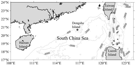
Figure 1.
Geographical Map of the South China Sea.
In the northern South China Sea, a significant amount of research has been conducted, systematically measuring ISW parameters. Ramp et al. [27] conducted combined moored and shipboard observations near the continental shelf break between the southern tip of Taiwan and Dongsha Island. They observed ISWs with amplitudes ranging from 29 to 142 m and propagation speeds between 0.83 and 1.84 m/s. Yang et al. [28] deployed thermistor chain moorings on the continental slope northeast of Dongsha Island and reported ISWs with an average amplitude of 90 ± 15 m and an average propagation speed of 1.52 ± 0.04 m/s, estimated using the Korteweg–de Vries (KdV) equation. Klymak et al. [2], using sonar and a fast conductivity–temperature–depth (CTD) profiler, observed an ISW with an amplitude of 170 m and a propagation speed of 2.9 ± 0.1 m/s in the deep basin west of the Luzon Strait. Ramp et al. [29] deployed four oceanographic moorings along a transect from the Batanes Province, Philippines, in the Luzon Strait to just north of Dongsha Island on the Chinese continental slope. They observed ISWs with amplitudes ranging from 20 to 200 m and average propagation speeds of 3.23 ± 0.31 m/s in the deep basin and 2.22 ± 0.18 m/s over the continental slope. Lien et al. [30] observed five large-amplitude ISWs on the Dongsha slope during a spring tide using both shipboard and moored acoustic Doppler current profiler and CTD instruments. They reported amplitudes ranging from 106 to 173 m and propagation speeds between 1.6 and 1.72 m/s. Chen et al. [31] conducted year-long mooring observations west of Dongsha Island on the northern shelf slope, observing ISWs with an average amplitude of 43 ± 17 m and a propagation speed estimated by KdV of 1.38 ± 0.14 m/s. Chang et al. [32] deployed two mooring systems east of Dongsha Island and recorded ISWs with amplitudes ranging from 76 to 125 m and propagation speeds between 1 and 1.5 m/s. Ramp et al. [33] deployed an array of oceanographic moorings and a distributed temperature-sensing cable over the eastern slope of Dongsha Island, observing ISWs with amplitudes ranging from 20 to 180 m and propagation speeds between 1.1 and 2.6 m/s. In summary, in situ observations provide accurate measurements of ISW parameters. However, due to the high cost of deployment and maintenance, achieving extensive, continuous acquisition of ISW parameters remains challenging, thereby limiting the analysis of their spatial variability.
Recent advances in satellite remote sensing, particularly regarding spatial coverage, revisit frequency, and resolution, have enabled the systematic observation of ISWs over broad oceanic regions. Although remote sensing cannot directly measure ISW parameters such as amplitude and wavelength, relationships between surface features and wave parameters can be established through physical models, thereby enabling parameter retrieval through remote sensing inversion.
Zheng et al. [34] derived a theoretical model of ISW radar imagery based on the two-layer KdV equation and used synthetic aperture radar (SAR) imagery to retrieve the amplitudes of five ISWs over the Portuguese continental shelf and in the South China Sea. The retrieval results were consistent with the in situ measurements. Chen et al. [35] extended the KdV equation to the Benjamin–Ono (BO) equation and retrieved the amplitude of an ISW in the deep-water region of the northern South China Sea using optical imagery. The retrieved amplitude value was in reasonable agreement with historical in situ isotherm profile measurements. Huang and Zhao [36] applied a continuously stratified KdV model to retrieve ISW parameters from optical imagery in the deep-water region of the northern South China Sea, achieving good consistency with moored in situ observations. Zhang et al. [37] combined optical and SAR imagery with a corrected two-layer nonlinear Schrödinger (NLS) equation to retrieve the amplitudes of four ISWs in the Wenchang area, east of Hainan Island. The retrieved values closely matched the observed amplitudes. Jia et al. [38] utilized two consecutive SAR images and the extended KdV (eKdV) equation for a two-layer fluid to retrieve the amplitude of an ISW in shallow waters southeast of Hainan Island. The result was in close agreement with values derived using the classic KdV model under continuous stratification. Xie et al. [39] used both the KdV and NLS equations for a two-layer fluid, together with optical imagery, to retrieve the amplitudes of seven ISWs near Dongsha Island. The results aligned well with concurrent mooring observations. Chen et al. [40] applied the KdV, eKdV, and BO models for a two-layer fluid to SAR imagery to retrieve the amplitude of an ISW in the deep-water region of the northeastern South China Sea, yielding results consistent with historical mooring observations and with those from the continuously stratified KdV model.
Current remote sensing inversion studies of ISWs in the South China Sea have primarily focused on demonstrating the applicability of parameter retrieval methods in localized regions, with only a few case studies available. Systematic investigations into extensive ISW parameter retrieval and the spatial variability of these parameters remain lacking. In addition, most studies employ internal wave models based on two-layer fluid assumptions, without fully accounting for the continuous stratification commonly present in real ocean environments. By contrast, continuously stratified models better represent actual oceanic conditions [40] and yield more accurate inversion results than two-layer models [38]. Moreover, most existing inversion studies concentrate on retrieving the ISW amplitude, whereas propagation speed retrieval remains understudied, thereby limiting comprehensive insights into ISW dynamics. Most theoretical models used in remote sensing inversions are based on the weakly nonlinear assumption, which assumes that the ISW amplitude is small compared with their intrinsic vertical scale [41,42]. However, models based on the weakly nonlinear assumption are inadequate to describe strongly nonlinear ISWs [4,43], which account for a large proportion of ISWs in in situ oceanic observations [44,45,46,47]. Therefore, theoretical models with strong nonlinearity are needed when retrieving the parameters of large-amplitude ISWs from remote sensing imagery.
The Dubreil–Jacotin–Long (DJL) equation is a fully nonlinear model that makes no assumptions about wavelength or amplitude. Its applicability to strongly nonlinear ISWs has been validated in laboratory experiments and it has been successfully applied to retrieve ISW parameters [48]. In this study, the DJL equation under continuous stratification is employed in combination with continuous optical remote sensing imagery to retrieve ISW parameters over a broad region of the northern South China Sea. This study facilitates the analysis of the spatial variability of ISW parameters and reveals their distribution patterns in the northern South China Sea, thereby facilitating a more comprehensive understanding of ISW dynamics and providing essential data support for future investigations in the region.
The remainder of this study is organized as follows: In Section 2, we introduce the satellite remote sensing data, the theoretical equations of ISWs, and the methods used to extract ISW parameters. In Section 3, we present the inversion results and spatial variation characteristics of ISW parameters in the northern South China Sea. In Section 4, we discuss the comparison between the inversion results and in situ observations and analyze a case of propagation and evolution of a particular ISW. In Section 5, we summarize the main conclusions.
2. Data and Methods
2.1. Satellite Remote Sensing Data and ISW Parameter Extraction
The satellite imagery used in this study was obtained from the FY-4B Geo High-speed Imager (GHI), with a spatial resolution of 250 m and a swath width of 2000 km. FY-4B is the first operational satellite in China’s new generation of geostationary meteorological satellites under the Fengyun-4 series. It was launched on 3 June 2021 and successfully positioned at 133°E on 11 April 2022. Operational data and application services began on 1 June 2022. Between 1 February and 5 March 2024, the satellite drifted from 133°E to 105°E, where it replaced FY-4A as the primary operational platform. Since March 5, FY-4B has resumed operational services at 105°E. The satellite’s advanced GHI instrument captures imagery over a 2000 × 2000 km2 area with spatial resolutions ranging from 250 to 2000 m and a temporal resolution of up to 1 min, enabling ISW propagation and evolution to be monitored in the northern South China Sea.
Figure 2a displays a 250 m resolution image from FY-4B GHI, captured at 04:02 UTC on 19 June 2023, following radiometric calibration, geometric correction, and cropping. The image clearly reveals the presence of an ISW. By analyzing the image intensity along the ISW crest line and its surroundings, the brightest points (indicated by the cyan dots in Figure 2a) are identified. A grayscale profile is then extracted perpendicular to the ISW crest (represented by the cyan oblique line in Figure 2a), as shown in the upper-left inset. In this profile, bright and dark stripes correspond to positive and negative peaks, respectively. The distance between these peaks, referred to as the peak-to-peak (PP) distance (), can be measured from the grayscale profile. The PP distance is closely related to the characteristic half-width of ISWs [34] and serves as a key parameter for the retrieval of ISWs [49].
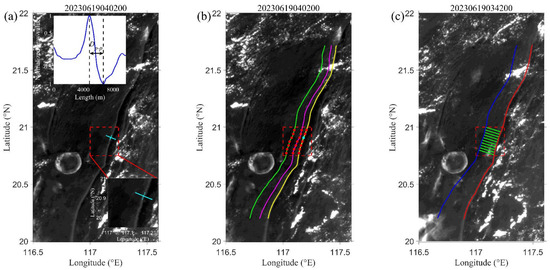
Figure 2.
FY-4B GHI imagery of the northern South China Sea. (a,b) Images captured at 04:02:00 UTC on 19 June 2023; (c) images captured at 03:42:00 UTC on the same day. In (a), cyan dots mark the brightest points of the ISW, and the cyan oblique line indicates the profile extraction path, perpendicular to the crest and opposite to the propagation direction. The lower-right inset enlarges the dashed rectangle, while the upper-left inset shows the grayscale profile with black dashed lines marking the horizontal positions of the maximum and minimum gray values. In (b), red dots show where PP distances are extracted; cyan dots correspond to those in (a). Yellow, purple, and green lines indicate ISW crests at 04:02, 05:02, and 06:02 UTC, respectively. In (c), the red line shows the crest at 03:42 UTC, the blue line shows its position at 06:42 UTC, and the green line shows the propagation path. Red dashed boxes denote 0.25° × 0.25° WOA grid cells.
Since the observation locations of FY-4B GHI vary daily, a total of 46 days between June 2022 and July 2024 were selected, during which ISWs in the northern South China Sea were clearly observed, as listed in Table 1. The daily observation time of ISWs was mainly concentrated between 00:00 and 09:00 UTC. The northern South China Sea is divided into grids with a resolution of 0.25°, consistent with the grid structure of the 0.25° temperature and salinity fields in the World Ocean Atlas 2023 (WOA23) dataset [50]. Figure 2b shows the propagation and evolution of ISWs over a continuous 3 h period. The PP distance of the ISWs in each grid is defined as the average value of the PP distances extracted from multiple ISW crest lines within that grid (as indicated by the red and cyan dots in Figure 2b). Figure 2c shows the positions of the ISW crest lines on the left and right sides of a single grid cell. The ISW propagation speed in each grid is defined as the average speed of all of the brightest points propagating from the right to the left side within that grid. The retrieval of ISW parameters is based on the PP distances and the temperature and salinity data from the WOA23 within each grid.

Table 1.
Summary of remote sensing imagery for ISW observations in the northern South China Sea.
2.2. ISW Theoretical Equations and Parameter Extraction
Without making any assumptions about wavelength or amplitude, the DJL equation [51,52] was established and is expressed as follows:
where represents the isopycnal displacement and is the propagation speed of ISWs. The Laplacian operator is defined as , and and denote the zonal and vertical coordinates, respectively. In this study, the ISW amplitude () retrieved using the DJL equation refers to the maximum isopycnal displacement, defined as follows:
in Equation (1) is the buoyancy frequency, given by the following:
where is the gravitational acceleration, is the density profile, and is the reference density. The density profiles were derived from WOA23 temperature and salinity profiles using the equation of state proposed by Millero and Poisson [53]. The temperature and salinity inputs used here are the monthly and seasonal averages of seven decadal means (1955–2022), with a spatial resolution of 0.25° × 0.25°. Seasonal data are applied at depths greater than 1500 m, while monthly data are used for depths less than 1500 m. It should be noted that the DJL equation does not have explicit solutions, which can only be solved by the numerical method [52,54].
When retrieving ISW parameters from optical imagery, it is important to account for the relationship between sea surface current divergence and the surface features of ISWs. Lu et al. [55] investigated the relationship using both satellite remote sensing and laboratory experiments. By statistically analyzing the ISW PP distances in optical imagery and the PP distances of the surface current divergence for the same ISW, and performing linear fitting, they found that the PP distance of the sea surface current divergence is 0.83 times that of the optical imagery. The experimental and remote sensing results are consistent. Furthermore, the uncertainty of this relationship is derived as 0.03. Since the maximum PP distance extracted from remote sensing imagery in this study is 3207 m, the error introduced by this relationship is 96 m, which is smaller than the image resolution. The error in the inversion amplitude due to the PP distance is 1 m, and the error in propagation speed is 0.004 m/s. Therefore, the error in this relationship has no significant impact on the inversion results.
The PP distance of the sea surface current divergence is defined as follows:
Therefore, the relationship between the ISW PP distance extracted from optical imagery () and the PP distance of the sea surface current divergence derived from the DJL theory () can be given by the following:
3. Results
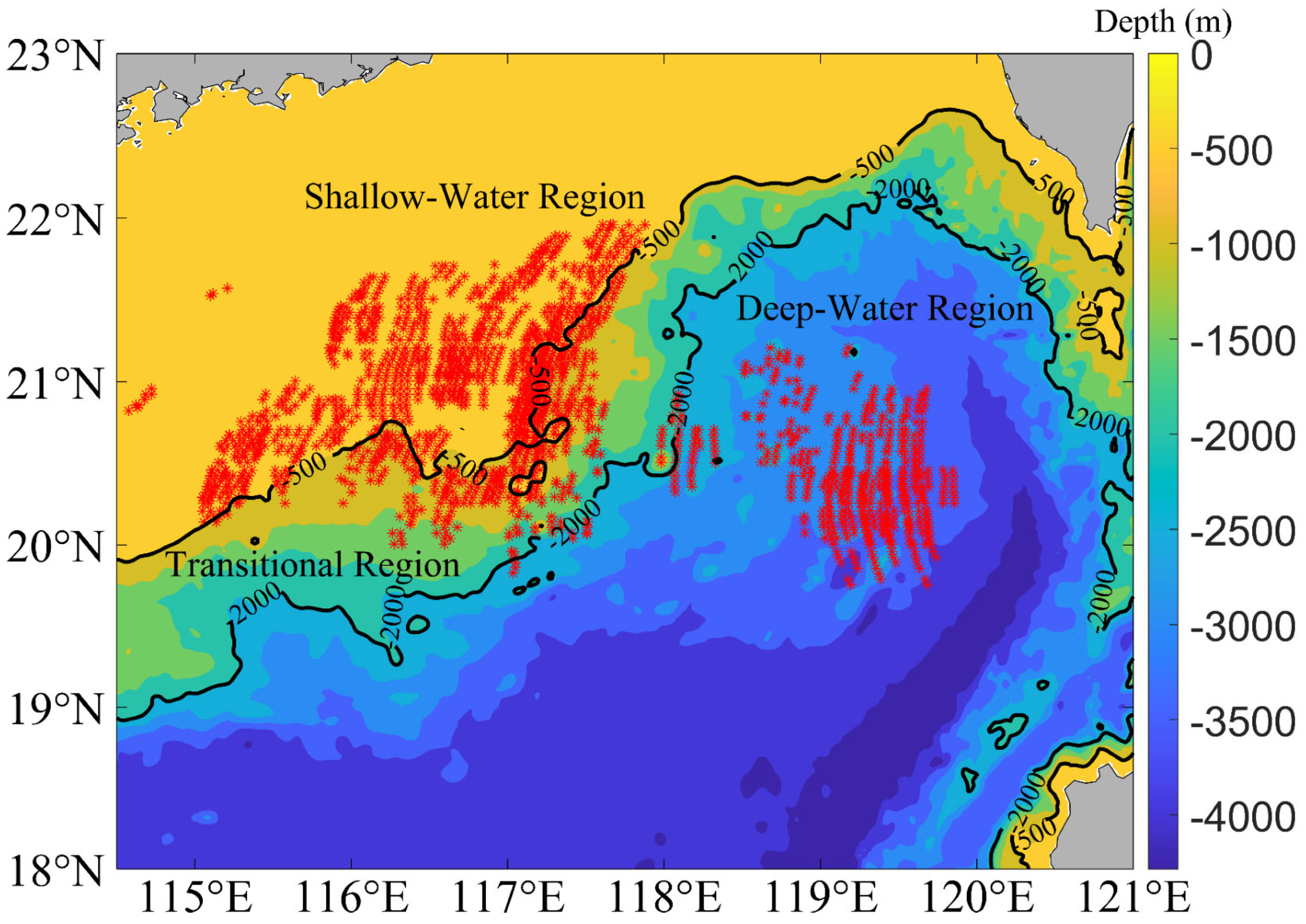
In this study, a total of 2067 ISW PP distances were extracted from 46 days of FY-4B GHI imagery that clearly captured ISWs in the northern South China Sea. The extraction locations are shown in Figure 3. The study area was divided into deep-water, transitional, and shallow-water regions based on the 500 m and 2000 m isobaths. Using the continuously stratified DJL equation and the extracted PP distances, ISW parameters in the northern South China Sea were retrieved, and their spatial variation characteristics were subsequently analyzed.
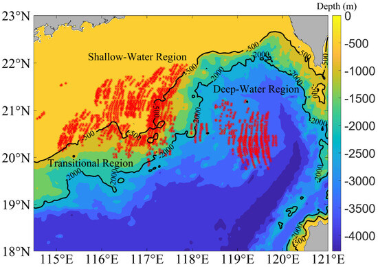
Figure 3.
Spatial distribution of ISW PP distance extraction locations in the northern South China Sea. Red asterisks mark the extraction points. Based on the 500 m and 2000 m isobaths, the region is divided into deep-water, transitional, and shallow-water regions.
3.1. Retrieval of ISW Parameters in the Deep-Water Region
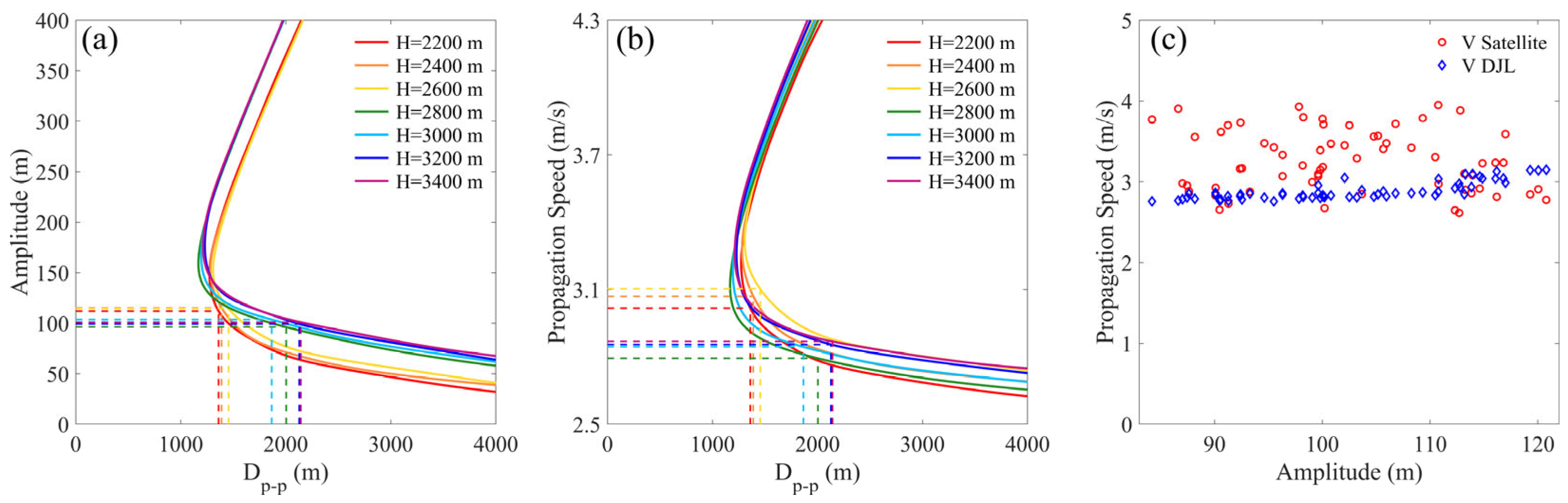
In the deep-water region, ISW parameters were retrieved using the continuously stratified DJL equation, driven by seasonal temperature and salinity data from WOA23. Figure 4a,b illustrate the relationships between the PP distance and amplitude and between the PP distance and propagation speed of ISWs, respectively, as derived from the DJL equation under different depth conditions. As shown, the relationship between the wave parameters and PP distance is no longer monotonic, and significant differences are exhibited when the amplitudes become large. Its typical feature is the existence of a turning point, which means that one PP distance will correspond to two parameters, that is, double solutions exist. Since it is difficult to distinguish between the two solutions using only the PP distance as a variable, Xue et al. [56] determined the double solutions based on the properties of wave packets in which the leading wave reaches the maximum amplitude. Instead, this study uses the ISW propagation speed estimated from continuous remote sensing imagery to more clearly determine whether to select the solution above or below the turning point. Once the propagation speed is determined, the corresponding amplitude is also fixed. By considering both the propagation speed and PP distance, the double solutions can be eliminated. Additionally, the selection of the double solutions can also be determined based on the historical measured data from the region. According to in situ observations by Huang et al. [57] in the deep-water region, the average ISW amplitude is typically less than 100 m. The turning point amplitude of the DJL solution in this region is always greater than 125 m. During their three-month continuous observations, a total of 177 ISWs were measured, of which only 4.5% had amplitudes exceeding 125 m. Therefore, the amplitudes below the turning point were selected, and the corresponding propagation speeds below the turning point were also chosen.
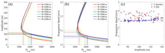
Figure 4.
(a,b) Relationships between ISW PP distance and amplitude (a) and between PP distance and propagation speed (b), as derived from the DJL equation under different depth conditions in the deep-water region. In (a,b), the red, orange, yellow, green, cyan, blue, and purple lines correspond to DJL solutions at depths of 2200, 2400, 2600, 2800, 3000, 3200, and 3400 m (H represents the total depth), respectively. The dashed lines in corresponding colors indicate the ISW PP distances extracted and the amplitudes and propagation speeds retrieved at their respective depths. (c) Variation in ISW propagation speed with amplitude in the deep-water region. Red circles indicate propagation speeds estimated from continuous satellite remote sensing imagery, and blue diamonds represent those retrieved using the DJL equation.
As shown in Figure 4a, the DJL model curves for the PP distance and amplitude exhibit distinct differences between the depth ranges of 2800–3400 m and 2200–2600 m. The ISWs in deeper waters (2800–3400 m) correspond to larger extracted PP distances than those in shallower waters (2200–2600 m). However, differences in the curves across the two depth ranges lead to only minor variations in the retrieved ISW amplitudes, despite the substantial differences in the PP distance. Figure 4b shows that the relationship between the PP distance and propagation speed displays only minor differences across different depths. Figure 4c compares the ISW propagation speed estimated from continuous satellite imagery with that retrieved using the DJL equation corresponding to solutions below the turning point. The results indicate that the remotely sensed propagation speed is generally greater than that retrieved from the DJL model. This discrepancy is similar to the in situ observations by Huang et al. [57], who found that the measured ISW propagation speeds in deep water were generally greater than the theoretical propagation speeds. This difference may be attributed to the proximity of the deep-water region to ISW generation sites. The surrounding area is an active region for background processes such as local tidal currents, internal tides, mesoscale eddies [47,57], and the Kuroshio [58]. As a result, ISWs in the deep-water region are more likely to be influenced by these processes. These background processes not only generate strong currents but also alter stratification, leading to deviations from the WOA climate mean profile. This study simulated the impact of stratification changes caused by an anticyclonic eddy with a 100 m amplitude on the ISW propagation speed retrieved using the DJL equation. The results showed that the stratification changes led to a 0.96 m/s increase in ISW propagation speed at a PP distance of 2500 m. The combined effects of background currents and stratification changes result in the difference between the ISW propagation speeds estimated from remote sensing and the theoretical propagation speeds in the deep-water region.
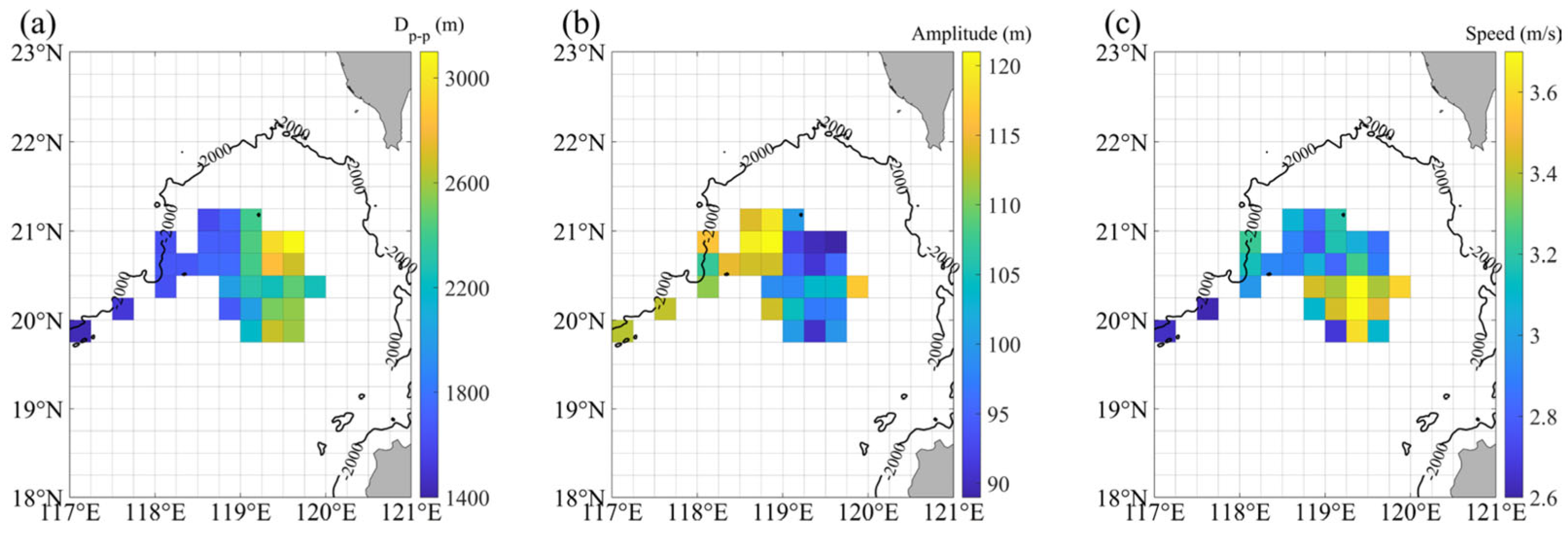
In the deep-water region (depths ranging from 2200 to 3400 m), a total of 555 ISW PP distances were extracted from continuous optical imagery, and the corresponding amplitudes and propagation speeds were retrieved using the continuously stratified DJL equation. The spatial distribution characteristics of the PP distance, amplitude, and propagation speed of ISWs are presented in Figure 5a–c. As shown in Figure 5a, the PP distance of ISWs, extracted from consecutive optical imagery, ranges from 1440 to 3087 m. From east (120°E) to west (117°E), the PP distances gradually decrease with decreasing depth. Figure 5b shows that the ISW amplitude ranges from 89 to 121 m, increasing gradually from east to west. Figure 5c indicates that the ISW propagation speeds range from 2.6 to 3.7 m/s. Influenced by background currents, these speeds are unevenly distributed, with slightly greater values observed in the southern portion of the study area.
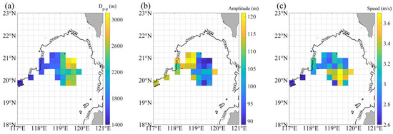
Figure 5.
(a) Spatial distribution of ISW PP distances extracted from optical imagery, (b) ISW amplitudes retrieved using the DJL theory, and (c) ISW propagation speeds estimated from continuous remote sensing imagery, all in the deep-water region. The grid resolution for (a–c) is 0.25°.
3.2. Retrieval of ISW Parameters in the Transitional Region
In the transitional region, the monthly and seasonal WOA23 temperature and salinity profiles were used to derive the continuously stratified DJL equation, from which the relationships between the ISW PP distance and amplitude (Figure 6a) and between the PP distance and propagation speed (Figure 6b) were derived at different depths. Based on the ISW propagation speed estimated from continuous remote sensing imagery, the DJL solution above or below the turning point corresponding to the same PP distance was selected. The results indicated that most of the DJL solutions corresponded to parameters above the turning point. For a few cases in which parameters were initially matched below the turning point, resulting in unrealistic amplitude outliers, the solution above the turning point was instead selected to ensure physical consistency.
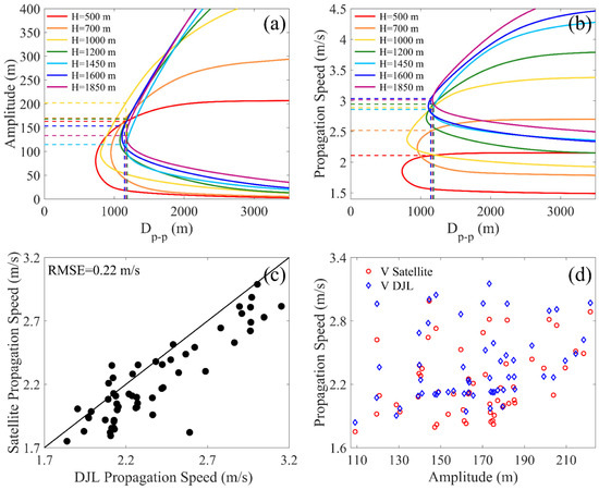
Figure 6.
(a,b) Relationships between ISW PP distance and amplitude (a) and between PP distance and propagation speed (b), as derived from the DJL equation at different depths in the transitional region. In (a,b), the red, orange, yellow, green, cyan, blue, and purple lines correspond to DJL solutions at depths of 2200, 2400, 2600, 2800, 3000, 3200, and 3400 m (H represents the total depth), respectively. The dashed lines in corresponding colors indicate the ISW PP distances extracted and the amplitudes and propagation speeds retrieved at their respective depths. (c) Comparison between ISW propagation speeds estimated from satellite remote sensing imagery and those retrieved using the DJL equation in the transitional region. RMSE denotes the root mean square error, and the solid black line represents the 1:1 reference. (d) Variations in ISW propagation speed with amplitude in the transitional region. Red circles indicate propagation speeds estimated from continuous satellite remote sensing imagery, and blue diamonds represent those retrieved using the DJL equation.
Figure 6a shows that the relationship between the ISW PP distance and amplitude, as derived from the DJL equation, exhibits significant variations at different depths. Although the PP distance of ISWs changes only slightly across this region, the retrieved amplitudes vary considerably. Figure 6b indicates that the curve of the propagation speed versus the PP distance derived from the DJL equation decreases as the depth becomes shallower. Given the relatively small variation in the PP distance, the propagation speed of ISWs progressively decreases as the water becomes shallower. As shown in Figure 6c, the ISW propagation speeds estimated from the continuous satellite remote sensing imagery closely match those retrieved from the DJL equation, with a root mean square error of 0.22 m/s. Figure 6d presents the variation in the ISW propagation speed with amplitude. The lack of a clear correlation suggests that depth may be the dominant factor influencing the ISW propagation speed in the transitional region.
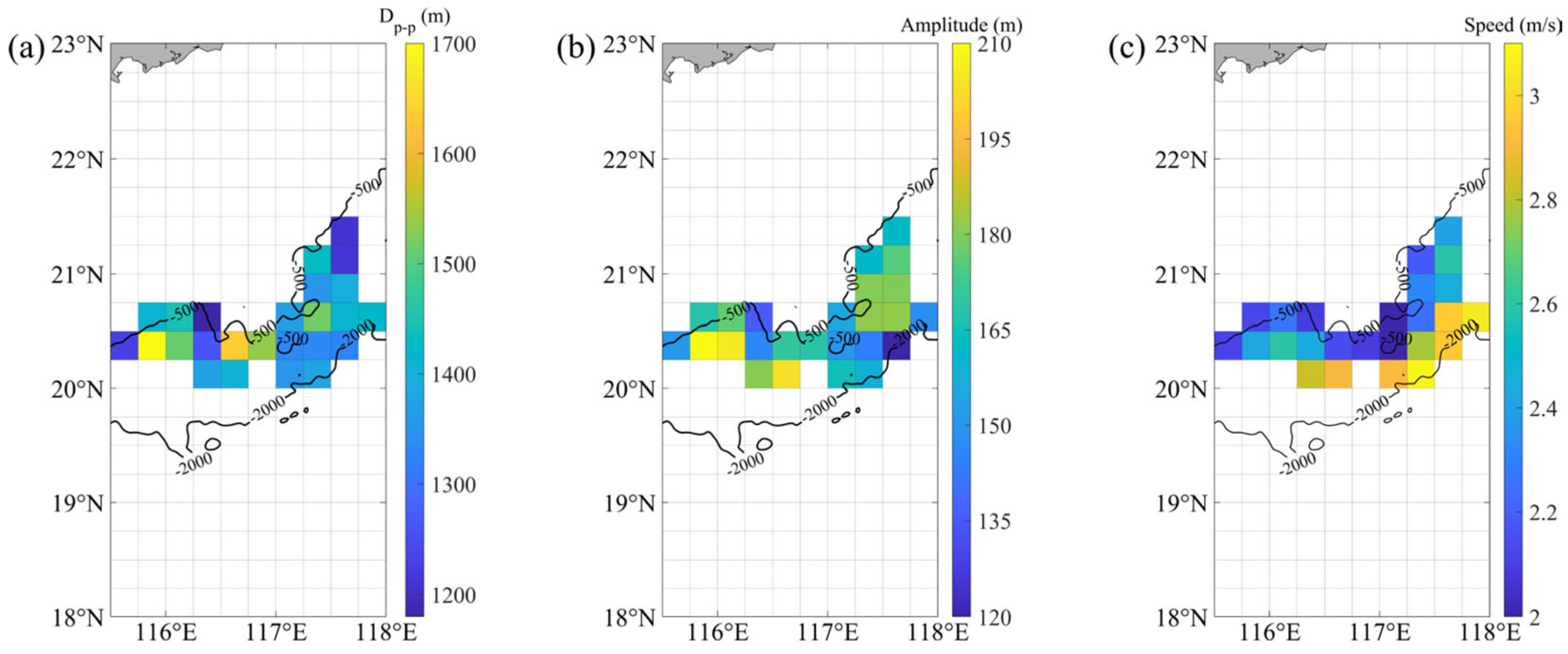
In the transitional region, where depths range from 500 to 1850 m, a total of 486 ISW PP distances were extracted from continuous optical imagery. Using the continuously stratified DJL equation, the corresponding amplitudes and propagation speeds were retrieved, and the spatial distributions of the PP distance, amplitude, and propagation speed were further analyzed (Figure 7a–c). Figure 7a shows that the ISW PP distances range from 1182 to 1697 m, with less variability compared to those in the deep-water region. As shown in Figure 7b, the ISW amplitudes retrieved using the DJL model range from 120 to 210 m, exceeding those retrieved in the deep-water region. These amplitudes are strongly influenced by depth and density, leading to significant variations. Figure 7c indicates that the propagation speeds retrieved using the DJL equation range from 2.0 to 3.1 m/s, and thus are lower than those in the deep-water region. Overall, ISWs in the transitional region exhibit shorter PP distances, greater amplitudes, and lower propagation speeds compared to those in the deep-water region.

Figure 7.
(a) Spatial distribution of ISW PP distances extracted from optical imagery, (b) ISW amplitudes retrieved using the DJL theory, and (c) ISW propagation speeds retrieved using the DJL theory, all in the transitional region. The grid resolution for (a–c) is 0.25°.
3.3. Retrieval of ISW Parameters in the Shallow-Water Region
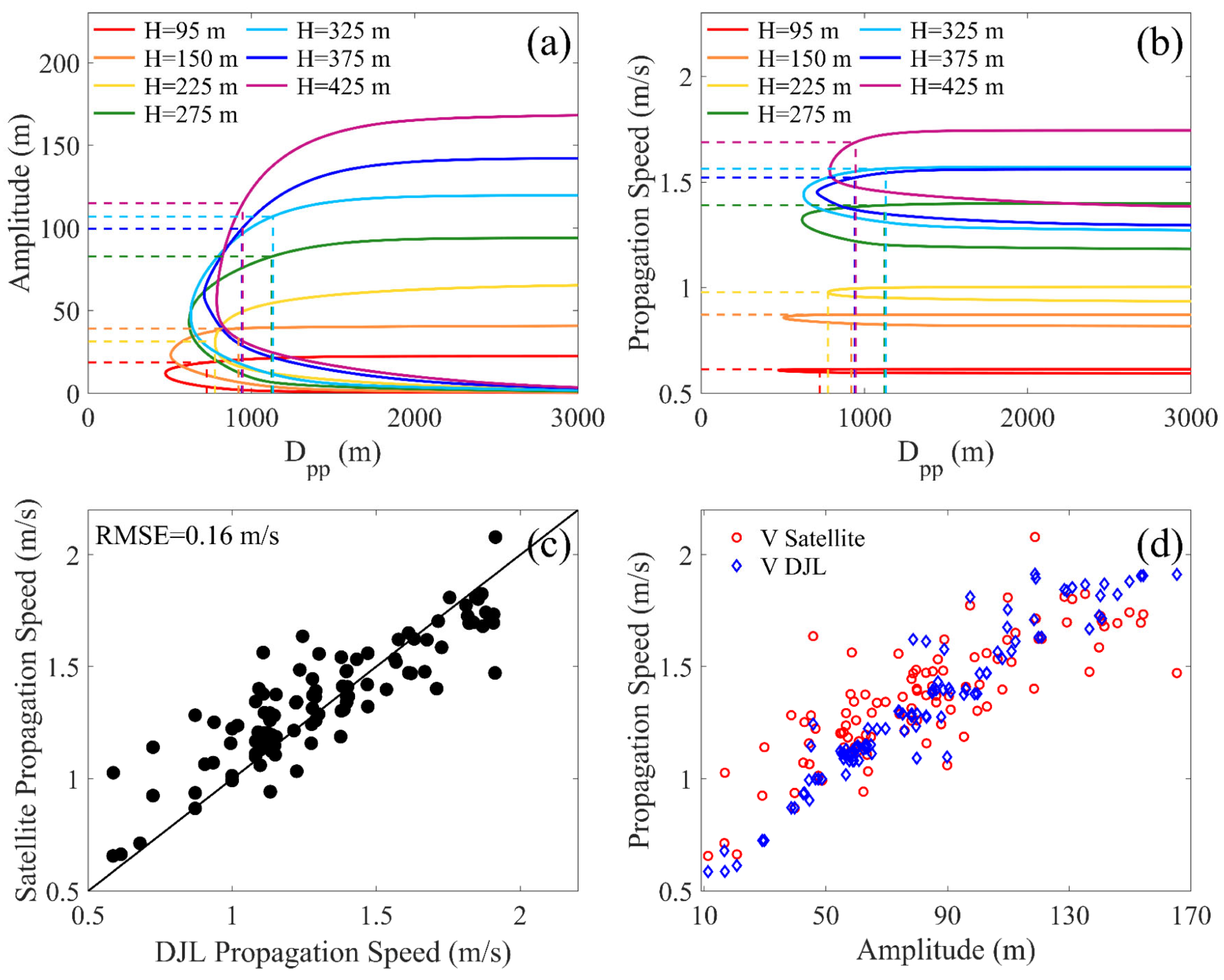
In the shallow-water region, the DJL equation was solved using monthly WOA23 temperature and salinity profiles. Figure 8a,b illustrate the relationships between the ISW PP distance and amplitude, and between the PP distance and propagation speed, respectively, as obtained from the DJL equation under varying depth conditions. The DJL solutions were likewise selected based on the propagation speeds estimated using the continuous remote sensing imagery. Similarly to the transitional region, most cases corresponded to parameters above the turning point. For the few cases with initial mismatches, appropriate corrections were applied to ensure physical consistency.
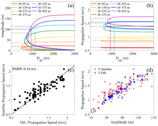
Figure 8.
(a,b) Relationships between ISW PP distance and amplitude (a) between and PP distance and propagation speed (b), as derived from the DJL equation under different depth conditions in the shallow-water region. In (a,b), the red, orange, yellow, green, cyan, blue, and purple lines correspond to DJL solutions at depths of 2200, 2400, 2600, 2800, 3000, 3200, and 3400 m (H represents the total depth), respectively. The dashed lines in corresponding colors indicate the ISW PP distances extracted and the amplitudes and propagation speeds retrieved at their respective depths. (c) Comparison between ISW propagation speeds estimated from satellite remote sensing imagery and those retrieved using the DJL equation in the shallow-water region. RMSE denotes the root mean square error, and the solid black line represents the 1:1 reference. (d) Variation in ISW propagation speed with amplitude in the shallow-water region. Red circles indicate propagation speeds estimated using continuous satellite remote sensing imagery, and blue diamonds represent those retrieved using the DJL equation.
Figure 8a,b show that, as the depth gradually decreases, both the relationship between the PP distance and amplitude and that between the PP distance and propagation speed, as retrieved using the DJL equation, exhibit a decreasing trend. Although the ISW PP distances vary under different depth conditions, the retrieved amplitudes and propagation speeds generally decrease as the depth becomes shallower. This suggests that in the shallow-water region, the ISW amplitude and propagation speed are strongly influenced by depth, with both parameters tending to decline as the depth decreases. Figure 8c presents a comparison between the ISW propagation speeds estimated using the continuous satellite imagery and those retrieved using the DJL equation, showing a good overall agreement, with a root mean square error of 0.16 m/s. Figure 8d illustrates that the ISW propagation speed increases with amplitude, indicating a positive correlation between the two in shallow waters.
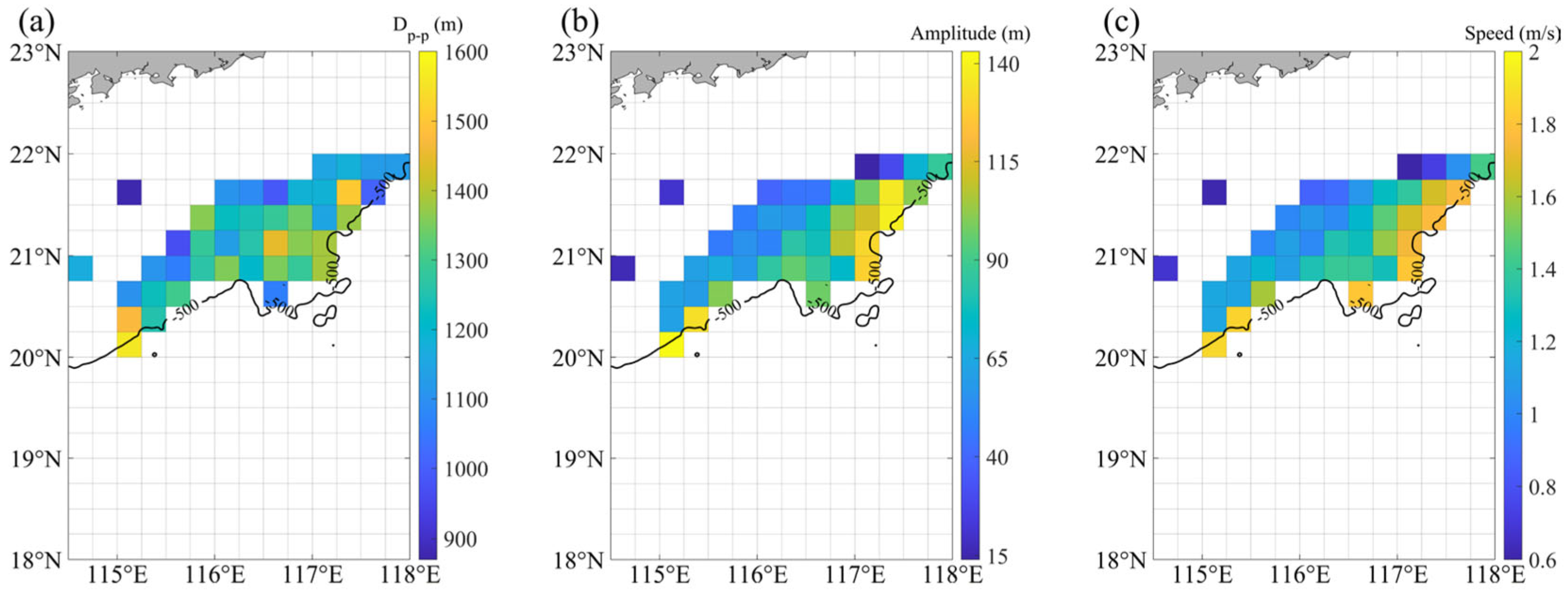
In the shallow-water region (depth range: 95–425 m), a total of 1026 ISW PP distances were extracted from the continuous optical imagery, and the corresponding amplitudes and propagation speeds were retrieved using the continuously stratified DJL equation. Figure 9a–c illustrate the spatial distributions of the ISW PP distance, amplitude, and propagation speed. As shown in Figure 9a, the ISW PP distances range from 876 to 1561 m, with only minor differences compared to those in the transitional region. Figure 9b shows that the ISW amplitudes, retrieved using the DJL model, range from 14 to 142 m, indicating a reduction relative to the transitional region. Figure 9c reveals that the ISW propagation speeds retrieved with the DJL equation range from 0.6 to 1.9 m/s, being lower than those in the transitional region. Overall, both the ISW amplitude and propagation speed decrease with decreasing depth, and all of the wave parameters are reduced compared to those in the transitional region.

Figure 9.
(a) Spatial distribution of ISW PP distances extracted from optical imagery, (b) ISW amplitudes retrieved using the DJL theory, and (c) ISW propagation speeds retrieved using the DJL theory, all in the shallow-water region. The grid resolution for (a–c) is 0.25°.
3.4. Spatial Variability of ISW Parameters in the Northern South China Sea
Using the continuously stratified DJL equation and continuous optical remote sensing imagery, the spatial distribution of ISW parameters across a depth range of 95–3400 m in the northern South China Sea was retrieved, as shown in Figure 10. Figure 10a illustrates that the ISW PP distances range from 876 to 3087 m, with the largest values observed in the deep-water region, where the average is 2134 m. As ISWs propagate westward, the PP distances decrease, averaging 1287 m. In the transitional and shallow-water regions, the PP distances show minimal variation. Figure 10b shows that the ISW amplitudes range from 14 to 210 m. In the deep-water region, the amplitudes remain relatively constant, averaging 102 m. As ISWs propagate westward into the transitional region, the intensified nonlinear effects lead to a notable increase in the amplitude. In the shallow-water region, the amplitudes gradually decrease with decreasing depth. Figure 10c indicates that the ISW propagation speeds range from 0.6 to 3.7 m/s, with the highest overall speeds in the deep-water region, where the average speed is 3.1 m/s. As ISWs propagate westward and the depth decreases, the propagation speeds decrease to an average of 2.3 m/s, and further reduce to 1.3 m/s in the shallow-water region.
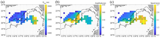
Figure 10.
Spatial distributions of (a) ISW PP distances, (b) ISW amplitudes, and (c) ISW propagation speeds in the northern South China Sea, respectively. The grid resolution for (a–c) is 0.25°.
4. Discussion
4.1. Impact of Seasonal Stratification Variations on the Retrieval of ISW Parameters
This study examines the impact of seasonal stratification variations on the retrieval of ISW parameters based on the DJL equation. In the deep-water region, for ISW PP distances between 2500 and 3500, the retrieval amplitude was smallest in summer and largest in winter, with the difference between winter and summer being approximately 20.5%. The retrieval propagation speed was lowest in spring and highest in summer, with the difference between spring and summer being approximately 6.5%. In the transition region, for ISW PP distances between 1500 and 2500, the retrieval amplitude was smallest in winter and largest in spring, with the difference between spring and winter ranging from 20% to 34%. The retrieval propagation speed was lowest in winter and highest in summer, with the difference between summer and winter being approximately 25.5%. In the shallow-water region, for ISW PP distances between 1500 and 2500, the seasonal variations in the retrieved wave parameters were similar to those in the transition region. The difference between spring and winter in the retrieval amplitude ranged from 37% to 50%, and the difference in retrieval propagation speed between summer and winter was approximately 27.5%. In summary, the impact of seasonal stratification variations on the retrieval of ISW parameters was significant, with the seasonal effect increasing as the depth decreased.
4.2. Comparison Between Retrieved ISW Parameters and In Situ Observations
The ISW parameters in the northern South China Sea were retrieved by combining continuous optical remote sensing imagery with the continuously stratified DJL equation, and the results were compared with in situ observations. In the deep-water region, Huang et al. [57] reported average in situ ISW amplitudes below 100 m and propagation speeds ranging from 2.8 to 3.7 m/s. In comparison, the retrieval using the DJL equation produced an average amplitude of 102 m, and the propagation speeds estimated from the remote sensing imagery ranged from 2.6 to 3.7 m/s.
In the transitional region, Lien et al. [30] conducted mooring observations at a depth of 525 m (117.28°E, 21.07°N), reporting ISW amplitudes of 106–173 m and propagation speeds of 1.61–1.98 m/s. At the same location, the ISW amplitudes retrieved using the DJL equation ranged from 130 to 204 m, with propagation speeds between 1.97 and 2.27 m/s. Similarly, Ramp et al. [33] measured an ISW amplitude of 100 m and a propagation speed of 1.8 m/s at a depth of 505 m (117.08°E, 20.7°N), while the results retrieved from the DJL equation at the same site ranged from 109 to 176 m in amplitude and from 1.84 to 2.13 m/s in speed.
In the shallow-water region, Yang et al. [28] reported ISW amplitudes of 90 ± 15 m and propagation speeds of 1.52 ± 0.04 m/s, estimated using the KdV equation, at a depth of 426 m (117.22°E, 21.05°N). At a nearby location, Lien et al. [30] measured amplitudes of 106–173 m and speeds of 1.61–1.9 m/s. The amplitudes retrieved using the DJL equation at the same site ranged from 120 to 146 m, with propagation speeds of 1.63–1.84 m/s. Additionally, Chen et al. [31] observed amplitudes ranging from 10 to 100 m and estimated propagation speeds using the KdV equation as being between 0.74 and 1.88 m/s at a depth of 397 m (115.5°E, 20.52°N), while the DJL equation retrieved amplitudes of 89 to 112 m and speeds of 1.58 to 1.61 m/s.
Overall, the retrieved ISW parameters using the DJL model showed good agreement with in situ observations across various regions, supporting the applicability and reliability of the DJL equation for ISW parameter retrieval in the northern South China Sea.
4.3. An Example of the Propagation and Evolution of a Particular ISW in the Northern South China Sea
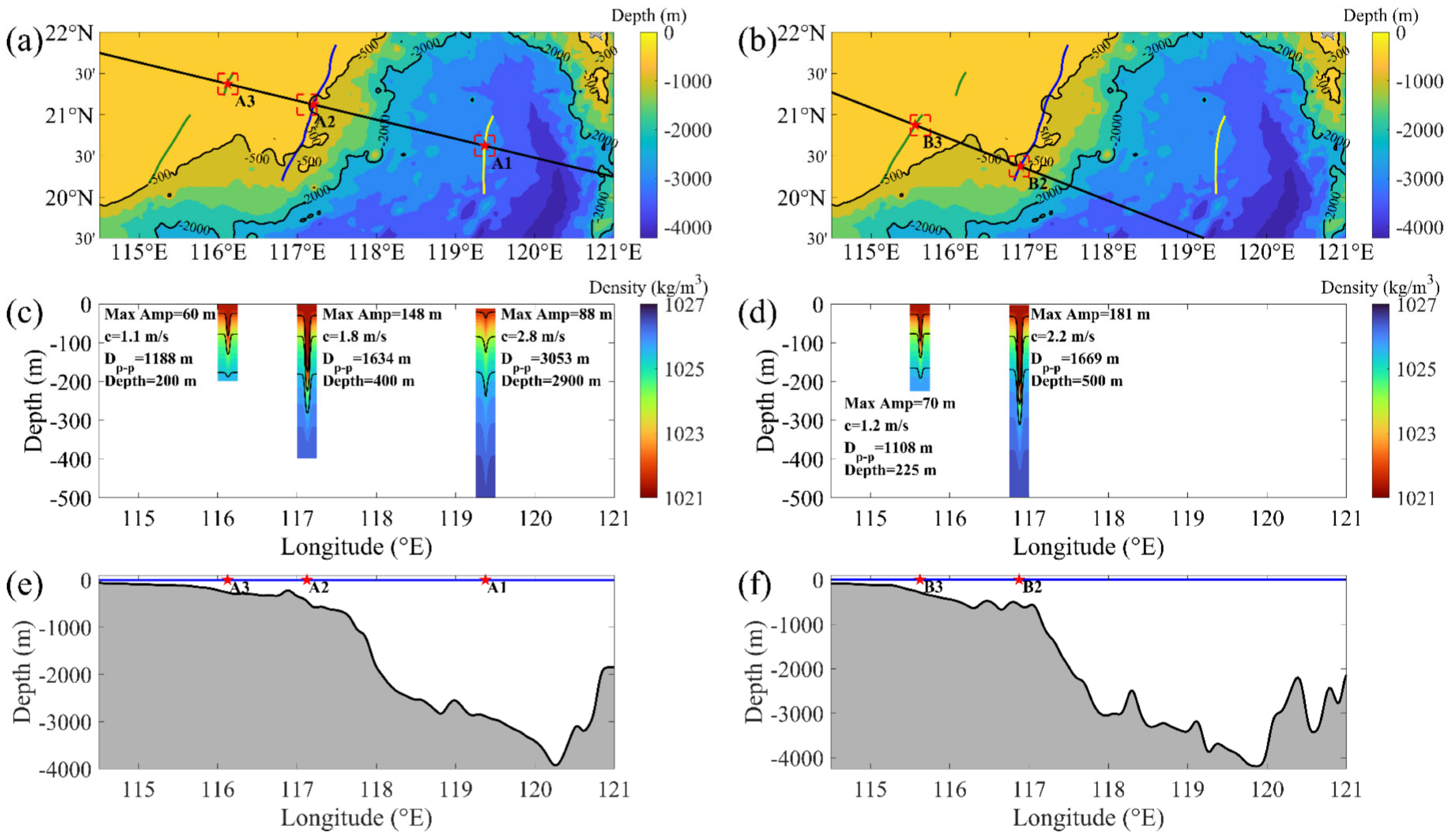
During the study period, the optical FY-4B GHI imagery featured the same ISW over three consecutive days. Using the continuously stratified DJL equation, the ISW’s parameters were retrieved from different regions, facilitating a systematic analysis of its propagation and evolution, as shown in Figure 11 At 04:51 UTC on 18 June 2023, the ISW was observed in the deep-water region at 119.37°E, 20.63°N (point A1 in Figure 11a), with a depth of 2900 m. The extracted ISW PP distance was 3053 m, with a maximum amplitude of 88 m and a propagation speed of 2.8 m/s, as retrieved using the DJL equation (Figure 11c). Along its northwestward propagation path (shown by the black diagonal line in Figure 11a), the ISW propagated into progressively shallower waters (Figure 11e). At 04:52 UTC on 19 June 2023, the ISW was observed at the junction of the transitional and shallow-water regions (117.21°E, 21.12°N; point A2 in Figure 11a). The depth was 400 m, with a PP distance of 1450 m, a maximum amplitude of 148 m, and a propagation speed of 1.8 m/s. Compared to the ISW at point A1, the ISW at point A2 was located in shallower water and exhibited a shorter PP distance, larger amplitude, and lower propagation speed, consistent with parameter variations observed from the deep-water to the transitional region. From A1 to A2, the ISW propagated for 232 km, yielding an average speed of 2.7 m/s, in good agreement with the mean propagation speed (2.7 m/s) of ISWs along the black solid line between the two points.
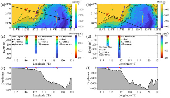
Figure 11.
(a,b): Propagation of the same ISW in the northern South China Sea. The background shows the bathymetry, with yellow, blue, and green lines representing wave crests extracted at three different times: 04:51:00 UTC on 18 June 2023 (yellow), 04:52:00 UTC on 19 June 2023 (blue), and 04:51:00 UTC on 20 June 2023 (green), respectively. Black diagonal lines represent the ISW propagation directions, and red pentagrams mark the intersection points between black lines and the wave crests. Red dashed boxes denote 0.25° × 0.25° areas corresponding to grid cells in the WOA23 dataset. (c,d): Isopycnal displacements calculated using the DJL equation. Background shading represents density variation. Black contours indicate the displacements of isopycnals with densities of 1022, 1024, and 1025.5 kg·m−3. (e,f): Bathymetric profiles along the propagation paths indicated by the black lines in panels (a,b), respectively. The blue line denotes the sea surface (0 m), and red pentagrams correspond to the same locations as in panels (a,b).
On the second day, as the ISW propagated and encountered Dongsha Island, it underwent refraction and split into two branches (indicated by the green diagonal lines in Figure 11a,b). One branch propagated through the shallow waters above the Dongsha Island and was observed at location A3 (116.12°E, 21.38°N) at 04:51 UTC on 20 June 2023. At this site, the depth was 200 m, the extracted ISW PP distance was 1188 m, and the retrieved maximum amplitude and propagation speed were 60 m and 1.1 m/s, respectively. At A3, the ISW was located in shallower water than at A2, with the PP distance, amplitude, and propagation speed all decreasing with decreasing depth, in agreement with the parameter variation trend observed in shallow-water regions. The ISW propagated 116 km from A2 to A3 at an average speed of 1.3 m/s, which closely matched the mean propagation speed (1.3 m/s) along the black solid line between A2 and A3 in the shallow-water region.
Another ISW propagated beneath Dongsha Island. On the second day, it was observed at location B2 (116.89°E, 20.38°N), where the depth was 500 m. The extracted PP distance was 1669 m, the maximum amplitude was 181 m, and the propagation speed was 2.2 m/s. Although B2 and A2 correspond to the same ISW, differences in the local depth and density structure resulted in variations in the PP distance, amplitude, and propagation speed. On the third day, the ISW was observed at B3 (115.56°E, 20.88°N), where the depth was 225 m. The extracted PP distance was 1108 m, and the maximum amplitude and propagation speed retrieved using the DJL equation were 70 m and 1.2 m/s, respectively. At B3, compared to B2, the ISW was located in shallower water, with a decrease in the PP distance, propagation speed, and amplitude, consistent with the trend observed from the transitional to shallow-water regions. From B2 to B3, the ISW propagated 149 km at an average speed of 1.7 m/s, closely matching the mean speed (1.8 m/s) along the black solid line between B2 and B3. Although the travel time from A2 to A3 and from B2 to B3 was the same, the ISW from B2 to B3 covered a 33 km longer distance, resulting in a higher average propagation speed. This difference was attributed to a greater average depth along the B2–B3 path compared to A2–A3 (as shown in Figure 11e,f), since shallower depths correspond to slower ISW speeds. Although A3 and B3 are located in different regions, the ISW parameters differed little due to the similar depths, supporting the conclusion that depth is the primary factor influencing ISW parameters in shallow-water regions. In summary, variations in the parameters of the same ISW across different regions were consistent with the spatial variation trends analyzed in Section 3.
The ISW propagated from deep water (A1) to shallow water (A3), with its amplitude initially increasing and then decreasing, which aligned with the in situ observations of Alford et al. [6]. Lamb and Warn-Varnas [59], using a two-dimensional non-hydrostatic primitive equation model, also found that as the depth decreases from 3000 m, the ISW amplitude increases significantly, reaching a maximum between 300 and 600 m, after which it rapidly decreases. In the deep-water region, the ISW was generated through the nonlinear steepening of internal tides in the Luzon Strait. As the ISW propagated westward, the nonlinear effects intensified. In the transitional region, influenced by the seafloor topography, the ISW shoaled and underwent steepening deformation, resulting in an increase in amplitude. As the ISW propagated into the shallow-water region, its energy dissipated due to shear, instability, and breaking, resulting in a decrease in amplitude.
The ISW propagation speed decreased as the depth decreased (A1 to A3), consistent with the in situ observations of Alford et al. [6], who showed that the ISW propagation speed decreased from deep water (3668 m) to shallow water (320 m). According to the ISW theory equation [60], the ISW propagation speed consists of two components: nonlinear and linear phase speeds. The nonlinear phase speed is primarily influenced by the wave amplitude, while the linear phase speed dominates and is mainly determined by depth, with higher speeds in deeper water. Therefore, as the ISW propagated from deep to shallow water, its propagation speed decreased with the reduction in depth. In the shallow-water region, where the linear phase speed was lower, the relative contribution of nonlinear effects on wave speed became more prominent.
5. Conclusions
In this study, ISW parameters in the northern South China Sea were retrieved by integrating continuous optical FY-4B GHI imagery using the DJL equation under continuous stratification. The retrieved parameters were used to characterize spatial variations in ISWs across deep-water, transitional, and shallow-water regions. The results showed that in the deep-water region, ISWs exhibited the greatest PP distances and propagation speeds among all regions, with mean values of 2134 m and 3.1 m/s, respectively, while the amplitudes showed only limited variability, with an average of 102 m. As ISWs propagated westward into the transitional region, the depth decreased and nonlinearity intensified. As a result, the PP distance and propagation speed decreased to average values of 1389 m and 2.3 m/s, respectively, while the amplitude increased, ranging from 120 to 210 m. In the shallow-water region, ISWs propagated northwestward. As the depth continued to decrease, the PP distance remained relatively constant (averaging 1227 m), while both the amplitude (ranging from 14 to 142 m) and propagation speed (averaging 1.3 m/s) gradually decreased with depth. Overall, in the northern South China Sea, the ISW PP distances ranged from 876 to 3087 m, exhibiting a decreasing trend from east to west. The amplitudes ranged from 14 to 210 m, increasing initially and then decreasing as ISWs propagated westward. The propagation speeds ranged from 0.6 to 3.7 m/s and declined progressively with decreasing depth.
In the inversion process, selecting appropriate DJL solutions is critical. Appropriate DJL solutions for each area, except for the deep-water region, can be determined from an analysis of the ISW propagation speeds estimated from continuous remote sensing imagery. In both transitional and shallow-water regions, most of the DJL solutions corresponded to parameters above the turning point. Comparisons with in situ measurements confirmed that the retrieved amplitudes and speeds were consistent with the field observations. This supports the validity and applicability of the proposed inversion framework when it is applied in the northern South China Sea. Furthermore, a three-day consecutive remote sensing tracking analysis of the same ISW revealed that the spatial variation in its parameters was consistent with the statistical results presented earlier. This study provides essential data support for understanding the spatial variability and dynamic characteristics of ISWs in the northern South China Sea and offers an effective remote sensing inversion method for future extensive ISW research and monitoring.
Author Contributions
Conceptualization, K.L., T.X., C.J. and X.C.; methodology, K.L., T.X., C.J. and X.C.; software, K.L. and T.X.; writing—original draft preparation, K.L.; writing—review and editing, K.L., T.X., C.J., X.C. and X.H. All authors have read and agreed to the published version of the manuscript.
Funding
This work was supported by the National Key Research and Development Program of China (grant no. 2024YFC2815704) and the National Natural Science Foundation of China (grant no. 42476012).
Data Availability Statement
FY-4B GHI optical remote sensing imagery was downloaded from http://satellite.nsmc.org.cn/DataPortal/cn/home/index.html (accessed on 20 May 2025). The World Ocean Atlas 2023 is available at https://www.ncei.noaa.gov/access/world-ocean-atlas-2023/ (accessed on 20 May 2025). The results presented in this paper are available at https://zenodo.org/records/15474353 (accessed on 20 May 2025).
Acknowledgments
Figures were made with Matlab version 2021a (The MathWorks Inc., Natick, MA, USA, 2021), available at https://www.mathworks.com (accessed on 20 May 2025).
Conflicts of Interest
The authors declare no conflicts of interest.
References
- Jackson, C.R. Internal wave detection using the Moderate Resolution Imaging Spectroradiometer (MODIS). J. Geophys. Res. Ocean. 2007, 112, C11012. [Google Scholar] [CrossRef]
- Klymak, J.M.; Pinkel, R.; Liu, C.-T.; Liu, A.K.; David, L. Prototypical solitons in the South China Sea. Geophys. Res. Lett. 2006, 33, 11. [Google Scholar] [CrossRef]
- Huang, X.; Chen, Z.; Zhao, W.; Zhang, Z.; Zhou, C.; Yang, Q.; Tian, J. An extreme internal solitary wave event observed in the northern South China Sea. Sci. Rep. 2016, 6, 30041. [Google Scholar] [CrossRef] [PubMed]
- Grue, J.; Jensen, A.; Rusås, P.-O.; Sveen, J.K. Properties of large-amplitude internal waves. J. Fluid Mech. 1999, 380, 257–278. [Google Scholar] [CrossRef]
- Lamb, K.G. A numerical investigation of solitary internal waves with trapped cores formed via shoaling. J. Fluid Mech. 2002, 451, 109–144. [Google Scholar] [CrossRef]
- Alford, M.H.; Lien, R.-C.; Simmons, H.; Klymak, J.; Ramp, S.; Yang, Y.J.; Tang, D.; Chang, M.-H. Speed and evolution of nonlinear internal waves transiting the South China Sea. J. Phys. Oceanogr. 2010, 40, 1338–1355. [Google Scholar] [CrossRef]
- da Silva, J.C.B.; New, A.L.; Magalhaes, J.M. On the structure and propagation of internal solitary waves generated at the Mascarene Plateau in the Indian Ocean. Deep Sea Res. Part I Oceanogr. Res. Pap. 2011, 58, 229–240. [Google Scholar] [CrossRef]
- Osborne, A.R.; Burch, T.L. Internal solitons in the Andaman Sea. Science 1980, 208, 451–460. [Google Scholar] [CrossRef]
- Xu, A.; Chen, X. A Strong Internal Solitary Wave with Extreme Velocity Captured Northeast of Dong-Sha Atoll in the Northern South China Sea. J. Mar. Sci. Eng. 2021, 9, 1277. [Google Scholar] [CrossRef]
- Purwandana, A.; Cuypers, Y. Characteristics of internal solitary waves in the Maluku Sea, Indonesia. Oceanologia 2023, 65, 333–342. [Google Scholar] [CrossRef]
- Tian, Z.; Jia, Y.; Du, Q.; Zhang, S.; Guo, X.; Tian, W.; Zhang, M.; Song, L. Shearing stress of shoaling internal solitary waves over the slope. Ocean Eng. 2021, 241, 110046. [Google Scholar] [CrossRef]
- Huang, S.; Huang, X.; Zhao, W.; Chang, Z.; Xu, X.; Yang, Q.; Tian, J. Shear instability in internal solitary waves in the northern South China Sea induced by multiscale background processes. J. Phys. Oceanogr. 2022, 52, 2975–2994. [Google Scholar] [CrossRef]
- Xu, J.; Xie, J.; Chen, Z.; Cai, S.; Long, X. Enhanced mixing induced by internal solitary waves in the South China Sea. Cont. Shelf Res. 2012, 49, 34–43. [Google Scholar] [CrossRef]
- Bian, C.; Ruan, X.; Wang, H.; Jiang, W.; Liu, X.; Jia, Y. Internal solitary waves enhancing turbulent mixing in the bottom boundary layer of continental slope. J. Mar. Syst. 2022, 236, 103805. [Google Scholar] [CrossRef]
- Chen, T.-Y.; Tai, J.-H.; Ko, C.-Y.; Hsieh, C.-H.; Chen, C.-C.; Jiao, N.; Liu, H.-B.; Shiah, F.-K. Nutrient pulses driven by internal solitary waves enhance heterotrophic bacterial growth in the South China Sea. Environ. Microbiol. 2016, 18, 4312–4323. [Google Scholar] [CrossRef] [PubMed]
- Reid, E.C.; DeCarlo, T.M.; Cohen, A.L.; Wong, G.T.; Lentz, S.J.; Safaie, A.; Hall, A.; Davis, K.A. Internal waves influence the thermal and nutrient environment on a shallow coral reef. Limnol. Oceanogr. 2019, 64, 1949–1965. [Google Scholar] [CrossRef]
- Dong, J.; Zhao, W.; Chen, H.; Meng, Z.; Shi, X.; Tian, J. Asymmetry of internal waves and its effects on the ecological environment observed in the northern South China Sea. Deep Sea Res. Part I Oceanogr. Res. Pap. 2015, 98, 94–101. [Google Scholar] [CrossRef]
- Woodson, C.B. The fate and impact of internal waves in nearshore ecosystems. Annu. Rev. Mar. Sci. 2018, 10, 421–441. [Google Scholar] [CrossRef]
- Badiey, M.; Wan, L.; Song, A. Three-dimensional mapping of evolving internal waves during the Shallow Water 2006 experiment. J. Acoust. Soc. Am. 2013, 134, EL7–EL13. [Google Scholar] [CrossRef]
- Apel, J.R.; Ostrovsky, L.A.; Stepanyants, Y.A.; Lynch, J.F. Internal solitons in the ocean and their effect on underwater sound. J. Acoust. Soc. Am. 2007, 121, 695–722. [Google Scholar] [CrossRef]
- Huang, M.; Gao, C.; Zhang, N. Numerical research on hydrodynamic characteristics and influence factors of underwater vehicle in internal solitary waves. Int. J. Offshore Polar Eng. 2023, 33, 27–35. [Google Scholar] [CrossRef]
- Cheng, L.; Du, P.; Hu, H.; Xie, Z.; Yuan, Z.; Kaidi, S.; Chen, X.; Xie, L.; Huang, X.; Wen, J. Control of underwater suspended vehicle to avoid ‘falling deep’ under the influence of internal solitary waves. Ships Offshore Struct. 2024, 19, 1349–1367. [Google Scholar] [CrossRef]
- Song, Z.J.; Teng, B.; Gou, Y.; Lu, L.; Shi, Z.M.; Xiao, Y.; Qu, Y. Comparisons of internal solitary wave and surface wave actions on marine structures and their responses. Appl. Ocean Res. 2011, 33, 120–129. [Google Scholar] [CrossRef]
- Cui, J.; Dong, S.; Wang, Z.; Han, X.; Yu, M. Experimental research on internal solitary waves interacting with moored floating structures. Mar. Struct. 2019, 67, 102641. [Google Scholar] [CrossRef]
- Lien, R.-C.; Tang, T.Y.; Chang, M.H.; D’Asaro, E.A. Energy of nonlinear internal waves in the South China Sea. Geophys. Res. Lett. 2005, 32, L05615. [Google Scholar] [CrossRef]
- Simmons, H.; Chang, M.-H.; Chang, Y.-T.; Chao, S.-Y.; Fringer, O.; Jackson, C.R.; Ko, D.S. Modeling and prediction of internal waves in the South China Sea. Oceanography 2011, 24, 88–99. Available online: https://www.jstor.org/stable/24861123 (accessed on 20 May 2025). [CrossRef]
- Ramp, S.R.; Tang, T.Y.; Duda, T.F.; Lynch, J.F.; Liu, A.K.; Chiu, C.-S.; Bahr, F.L.; Kim, H.R.; Yang, Y.J. Internal solitons in the northeastern South China Sea. Part I: Sources and deep water propagation. IEEE J. Ocean. Eng. 2004, 29, 1157–1181. [Google Scholar] [CrossRef]
- Yang, Y.-J.; Tang, T.Y.; Chang, M.H.; Liu, A.K.; Hsu, M.-K.; Ramp, S.R. Solitons northeast of Tung-Sha Island during the ASIAEX pilot studies. IEEE J. Ocean. Eng. 2004, 29, 1182–1199. [Google Scholar] [CrossRef]
- Ramp, S.R.; Yang, Y.J.; Bahr, F.L. Characterizing the nonlinear internal wave climate in the northeastern South China Sea. Nonlinear Process. Geophys. 2010, 17, 481–498. [Google Scholar] [CrossRef]
- Lien, R.-C.; Henyey, F.; Ma, B.; Yang, Y.J. Large-amplitude internal solitary waves observed in the northern South China Sea: Properties and energetics. J. Phys. Oceanogr. 2014, 44, 1095–1115. [Google Scholar] [CrossRef]
- Chen, L.; Zheng, Q.; Xiong, X.; Yuan, Y.; Xie, H.; Guo, Y.; Yu, L.; Yun, S. Dynamic and statistical features of internal solitary waves on the continental slope in the northern South China Sea derived from mooring observations. J. Geophys. Res. Ocean. 2019, 124, 4078–4097. [Google Scholar] [CrossRef]
- Chang, M.-H.; Cheng, Y.-H.; Yang, Y.J.; Jan, S.; Ramp, S.R.; Reeder, D.B.; Hsieh, W.-T.; Ko, D.S.; Davis, K.A.; Shao, H.-J.; et al. Direct measurements reveal instabilities and turbulence within large amplitude internal solitary waves beneath the ocean. Commun. Earth Environ. 2021, 2, 15. [Google Scholar] [CrossRef]
- Ramp, S.R.; Yang, Y.-J.; Jan, S.; Chang, M.-H.; Davis, K.A.; Sinnett, G.; Bahr, F.L.; Reeder, D.B.; Ko, D.S.; Pawlak, G. Solitary waves impinging on an isolated tropical reef: Arrival patterns and wave transformation under shoaling. J. Geophys. Res. Ocean. 2022, 127, e2021JC017781. [Google Scholar] [CrossRef]
- Zheng, Q.; Yuan, Y.; Klemas, V.; Yan, X.-H. Theoretical expression for an ocean internal soliton synthetic aperture radar image and determination of the soliton characteristic half width. J. Geophys. Res. Ocean. 2001, 106, 31415–31423. [Google Scholar] [CrossRef]
- Chen, G.-Y.; Su, F.-C.; Wang, C.-M.; Liu, C.-T.; Tseng, R.-S. Derivation of internal solitary wave amplitude in the South China Sea deep basin from satellite images. J. Oceanogr. 2011, 67, 689–697. [Google Scholar] [CrossRef]
- Huang, X.; Zhao, W. Information of Internal Solitary Wave Extracted from MODIS Image: A Case in the Deep Water of Northern South China Sea. Period. Ocean Univ. China 2014, 44, 19–23. [Google Scholar]
- Zhang, X.; Wang, J.; Sun, L.; Meng, J. Study on the amplitude inversion of internal waves at Wenchang area of the South China Sea. Acta Oceanol. Sin. 2016, 35, 14–19. [Google Scholar] [CrossRef]
- Jia, T.; Liang, J.; Li, X.-M.; Fan, K. Retrieval of internal solitary wave amplitude in shallow water by tandem spaceborne SAR. Remote Sens. 2019, 11, 1706. [Google Scholar] [CrossRef]
- Xie, H.; Xu, Q.; Zheng, Q.; Xiong, X.; Ye, X.; Cheng, Y. Assessment of theoretical approaches to derivation of internal solitary wave parameters from multi-satellite images near the Dongsha Atoll of the South China Sea. Acta Oceanol. Sin. 2022, 41, 137–145. [Google Scholar] [CrossRef]
- Chen, H.; Wang, Z.; Cui, J.; Xia, H.; Guo, W. Application of different internal solitary wave theories for SAR remote sensing inversion in the northern South China Sea. Ocean Eng. 2023, 283, 115015. [Google Scholar] [CrossRef]
- Choi, W.; Camassa, R. Fully nonlinear internal waves in a two-fluid system. J. Fluid Mech. 1999, 396, 1–36. [Google Scholar] [CrossRef]
- Helfrich, K.R.; Melville, W.K. Long nonlinear internal waves. Annu. Rev. Fluid Mech. 2006, 38, 395–425. [Google Scholar] [CrossRef]
- Grue, J.; Jensen, A.; Rusås, P.-O.; Sveen, J.K. Breaking and broadening of internal solitary waves. J. Fluid Mech. 2000, 413, 181–217. [Google Scholar] [CrossRef]
- Stanton, T.P.; Ostrovsky, L.A. Observations of highly nonlinear internal solitons over the continental shelf. Geophys. Res. Lett. 1998, 25, 2695–2698. [Google Scholar] [CrossRef]
- Chang, M.-H.; Lien, R.-C.; Lamb, K.G.; Diamessis, P.J. Long-term observations of shoaling internal solitary waves in the Northern South China Sea. J. Geophys. Res. Ocean. 2021, 126, e2020JC017129. [Google Scholar] [CrossRef]
- Yang, Y.; Huang, X.; Zhao, W.; Zhou, C.; Huang, S.; Zhang, Z.; Tian, J. Internal solitary Waves in the Andaman Sea revealed by longterm mooring observations. J. Phys. Oceanogr. 2021, 51, 3609–3627. [Google Scholar] [CrossRef]
- Huang, X.; Huang, S.; Zhao, W.; Zhang, Z.; Zhou, C.; Tian, J. Temporal variability of internal solitary waves in the northern South China Sea revealed by long-term mooring observations. Prog. Oceanogr. 2022, 201, 102716. [Google Scholar] [CrossRef]
- Xu, T.; Chen, X.; Li, Q.; He, X.; Wang, J.; Meng, J. Strongly nonlinear effects on determining internal solitary wave parameters from surface signatures with potential for remote sensing applications. Geophys. Res. Lett. 2023, 50, e2023GL105814. [Google Scholar] [CrossRef]
- Zhang, X.; Wang, H.; Wang, S.; Liu, Y.; Yu, W.; Wang, J.; Xu, Q.; Li, X. Oceanic internal wave amplitude retrieval from satellite images based on a data-driven transfer learning model. Remote Sens. Environ. 2022, 272, 112940. [Google Scholar] [CrossRef]
- Reagan, J.R.; Boyer, T.P.; García, H.E.; Locarnini, R.A.; Baranova, O.K.; Bouchard, C.; Cross, S.L.; Mishonov, A.V.; Paver, C.R.; Seidov, D.; et al. World Ocean Atlas 2023; NOAA National Centers for Environmental Information: Silver Spring, MD, USA, 2024. Available online: https://www.ncei.noaa.gov/products/world-ocean-atlas (accessed on 20 May 2025).
- Long, R.R. Some aspects of the flow of stratified fluids: I. A theoretical investigation. Tellus 1953, 5, 42–58. [Google Scholar] [CrossRef]
- Stastna, M.; Lamb, K.G. Large fully nonlinear internal solitary waves: The effect of background current. Phys. Fluids 2002, 14, 2987–2999. [Google Scholar] [CrossRef]
- Millero, F.J.; Poisson, A. International one-atmosphere equation of state of seawater. Deep Sea Res. Part A Oceanogr. Res. Pap. 1981, 28, 625–629. [Google Scholar] [CrossRef]
- Dunphy, M.; Subich, C.; Stastna, M. Spectral methods for internal waves: Indistinguishable density profiles and double-humped solitary waves. Nonlinear Process. Geophys. 2011, 18, 351–358. [Google Scholar] [CrossRef]
- Lu, K.; Xu, T.; Chen, X.; He, X.; Tan, J. Relationships between internal solitary wave surface features in optical and SAR satellite images: Insights from remote sensing and laboratory. Ocean Eng. 2024, 309, 118500. [Google Scholar] [CrossRef]
- Xue, J.; Graber, H.C.; Lund, B.; Romeiser, R. Amplitudes estimation of large internal solitary waves in the Mid-Atlantic Bight using synthetic aperture radar and marine X-band radar images. IEEE Trans. Geosci. Remote Sens. 2012, 51, 3250–3258. [Google Scholar] [CrossRef]
- Huang, X.; Zhang, Z.; Zhang, X.; Qian, H.; Zhao, W.; Tian, J. Impacts of a mesoscale eddy pair on internal solitary waves in the northern South China Sea revealed by mooring array observations. J. Phys. Oceanogr. 2017, 47, 1539–1554. [Google Scholar] [CrossRef]
- Yu, Y.; Chen, X.; Cao, A.; Meng, J.; Yang, X.; Liu, T. Modulation of internal solitary waves by the Kuroshio in the northern South China Sea. Sci. Rep. 2023, 13, 6070. [Google Scholar] [CrossRef]
- Lamb, K.G.; Warn-Varnas, A. Two-dimensional numerical simulations of shoaling internal solitary waves at the ASIAEX site in the South China Sea. Nonlinear Process. Geophys. 2015, 22, 289–312. [Google Scholar] [CrossRef]
- Korteweg, D.J.; de Vries, G. On the change of form of long waves advancing in a rectangular canal, and on a new type of long stationary waves. Lond. Edinb. Dublin Philos. Mag. J. Sci. 1895, 39, 422–443. [Google Scholar] [CrossRef]


Disclaimer/Publisher’s Note: The statements, opinions and data contained in all publications are solely those of the individual author(s) and contributor(s) and not of MDPI and/or the editor(s). MDPI and/or the editor(s) disclaim responsibility for any injury to people or property resulting from any ideas, methods, instructions or products referred to in the content. |
© 2025 by the authors. Licensee MDPI, Basel, Switzerland. This article is an open access article distributed under the terms and conditions of the Creative Commons Attribution (CC BY) license (https://creativecommons.org/licenses/by/4.0/).