Abstract
Erosion is a powerful force that has moulded the Earth ever since water has been present on its rocky surface. In its seemingly harmless pursuit, erosion threatens ecosystems, reduces agricultural production, and impacts water quality. When trying to investigate erosion, there is no easy way to identify hotspots, only leaving the possibility of predicting where erosion should be occurring. This study aimed to develop a method to identify erosion using Synthetic Aperture Radar (SAR) images in a process called Coherent Change Detection (CCD). In doing so, it was found that CCD can be used to identify erosion due to rain events; however, false positives were also found due to soil moisture changes. This study used a new method for removing soil moisture effects that utilised the drying out of the soil to map where changes had occurred. This helped limit false positives, but more work is required to ensure soil moisture does not interfere with the results. Field data comprising aerial imagery and soil sampling were collected to improve the SAR processing as well as validate the results. The results of this study indicate the feasibility of developing an erosion analysis system capable of providing near real-time data specifically for arid regions.
1. Introduction
For millions of years, the unrelenting power of erosion has carved and sculpted the world. It stimulates soil formation, shapes geological features, influences sediment transportation, and initiates carbon storage. However, erosion also threatens ecosystems, reduces agricultural production, and overall represents a loss of a non-renewable resource. In fact, erosion has been noted as the largest widespread threat to the environment [1,2]. In particular, soil erosion causes 75 billion metric tons of soil to be displaced each year around the world [3]. Due to anthropogenic activities, rain events now pose an increased risk of irreparable soil erosion. As such, it is imperative to identify hotspots of erosion caused by rain events, allowing targeted mitigation strategies to be implemented.
A significant portion of Australia’s soil is old and weathered, leaving it vulnerable to erosion, something that significantly impacts Australia’s $90 Billion agricultural industry [4,5]. Studies have found that a 10 cm loss of soil could result in an $18 billion dollar impact on the industry [6,7,8]. Additionally, erosion affects the quality of surrounding waterways. The increased turbidity from suspended soil particles can block sunlight from reaching the river bed, while nitrogen and phosphorus found in some soils can cause eutrophication [9,10]. Together, these can decimate river ecosystems, which are the lifeblood of outback Australia [11]. Soil erosion and deposition can also alter the natural flow of water, causing flooding in areas that would not normally receive water while leaving others dry. Through these limited examples, it is clear the significant impact erosion can cause and why it needs to be closely monitored.
Despite its detrimental effects, the identification and monitoring of erosion is an arduous practice, particularly at large scales. The current erosion identification/monitoring techniques can be split into two categories, namely, predictive models and observational erosion analysis. Predictive models use erosion risk factors like slope, rainfall intensity, and land cover, to try and predict where erosion is likely to occur in an area [12]. The most popular predictive model is the Revised Universal Soil Loss Equation (RUSLE) developed by the United States Department of Agriculture, which was released to the public in 1992 [13]. Other studies have been completed using various predictive models ranging from looking at the multispectral signal of eroded areas to using land classification indexes to find gullies [14,15,16,17]. These models, like all other predictive models, are great for informing policy on a large scale but do not help accurately map erosion as it happens. This can only be completed using observational techniques, which are any processes where actual erosion is measured. Some examples of this are field studies and satellite data [18]. Field studies involve looking for evidence of erosion or using erosion plots to determine impacts in a small area. These studies are expensive and labour-intensive whilst only gaining data for a small area [19]. Satellite images can also be used by comparing different epochs to find any changes on the ground. Again, this method involves a large amount of human data interpretation and often does not reveal the full degree of erosion. More recently, a new technique of erosion analysis has been developed using Synthetic Aperture Radar (SAR) images to complete a CCD study [20].
Synthetic Aperture Radar (SAR) is a satellite observation technique that can observe changes in the earth’s surface [21]. SAR sensors emit radar waves towards the earth, measuring the intensity and phase difference in the backscattered wave. When readings from two different epochs are compared, changes in the earth’s surface can be identified [22]. When comparing SAR images from different epochs, coherence is used to assess the correlation between backscatter signals, highlighting areas where the backscattering changes. Equation (1) is used to calculate coherence [23].
where and are the complex pixel values of each of the SAR images and the angular brackets represent ensemble averaging. Using this equation results in a value from 0 to 1, with 1 being a strong correlation between the two epochs and 0 being no correlation. The factors that contribute to correlation can be split into four categories, being geometric, volumetric, thermal, and temporal [23,24,25].
The geometric factor refers to the distance between the satellite’s position at each epoch, known as the baseline. Any value greater than zero will create additional decorrelation; however, values of less than a few hundred metres result in an insignificant effect [25,26]. Volumetric decorrelation is the most common and occurs when radar waves bounce off multiple surfaces before returning to the satellite. This is often caused by vegetation but can also be the result of soil moisture, buildings, gullies, and other influences [27]. As long as there have been no changes in these factors between the two epochs, extra decorrelation should not occur. The third factor is thermal and is largely due to random errors of the receiver and, as such, cannot be easily adjusted for [24]. The last factor is temporal; changes due to temporal factors are often what studies are examining, looking for any changes in the ground surface between epochs. This is where the change detection part is established. Using coherence values between pairs and comparing these values to other pairs, the temporal effects on decorrelation can be studied. This allows for changes in the ground surface structure to be highlighted at particular periods of time.
CCD is particularly useful for finding erosion as it can be used in all weather conditions over large areas, has a sizable amount of historical data, and can detect small changes in surface structure. As SAR is an active sensor, it can be used to detect changes through cloud cover and at any time of the day. This is extremely beneficial when trying to investigate rain events where cloud cover is likely. Many methods used to investigate erosion are limited in scope, only being possible in small areas, whilst remote-sensing techniques offer the ability to investigate the entire earth due to their space-borne nature and significant history of data. Lastly, when measuring erosion, CCD can measure small changes in the surface structure. This is due to the nature of backscattered waves. If the ground is disturbed, it will reflect a different signal than the previous epoch, allowing any such changes to be detected in a coherence image. One disadvantage of coherence is that some areas will always have a low coherence due to vegetation or gullies. However, this has been overcome by calculating the background coherence of an area and correcting for the impact of vegetation and gullies.
To the best of the authors’ knowledge, only a limited number of studies have been performed using CCD to measure erosion, with only one being completed in Australia [28] and one other being used in Chile to measure erosion from rain events [20]. These studies both used very different techniques. The study in Australia was completed by Castellazzi et al., 2023 [28] and aimed at mapping gully erosion using CCD. It used a novel technique of creating large stacks using a small baseline subset (SBAS) method, creating a separate stack for dry and rainy conditions. Using this method, a large amount of data from the dry stack was used to estimate the background coherence, giving a highly accurate result. From this stack, the average and standard deviation for each pixel per temporal baseline were established. This is another advantage of the SBAS method as it allows a comparison between different temporal baselines. The background coherence was then used with the rain stack to highlight areas of erosion using a complex relationship between the two. Although using an SBAS method can give more accurate results, it also requires significant computer power and labour to complete the processing. As one proposed benefit of CCD is the reduced labour required, the need for computing power and human interaction with this method could be improved upon. The study from Chile completed by Cabré et al. (2020) [20] uses a much simpler method.
Cabré et al. (2020) [20] studied the erosion caused by a single rain event in the Atacama Desert using CCD. They used five coherence pairs with the same temporal baseline before the rain event to establish the average and standard deviation. They then determined the 95% confidence interval of each pixel and removed all values except the lower 2.5 percentile. Thus, this should only highlight areas that are very likely to have changed. The method used has a lower computational requirement; however. it did not validate its data successfully, only showing small areas that were examined during a field study.
This study aimed to refine the approach of previous work by proposing a method more rigorous than that used by Cabre et al. (2020) [20], but not as computationally heavy as Castellazzi et al., 2023 [28] and will provide a well-established validation of the results. This will be achieved by using fewer coherence pairs to estimate background coherence and correcting for still water and moisture changes while still utilising a streamlined approach.
2. Materials and Methods
2.1. Study Area and Data
The study area chosen was near Quilpie (in south-western Queensland, Australia), surrounding the Bulloo River, and spans an area of 12,000 km2 (Figure 1a). Colloquially, it is known as channel country due to the flatness of the land, with the only changes being the large channels the rivers create. In these areas, it rarely rains, with this region receiving less than 300 mm of rain each year [29]. However, when it does rain, it does so with high intensity, often causing widespread flooding [30]. Considering the significant flood events and the sandy soils of the area, this region experiences considerable erosion. Due to the remote nature of the land, this erosion often goes unnoticed and can cause significant environmental impacts. In 2022, this region and its catchment experienced higher than average rainfall as seen in Figure 1b. Figure 1b also shows the river levels as erosion may often be caused by rainfall from the catchment further north. One large rain event is evident on 2 February 2022. This rain was the first significant event in Quilpie since March 2020 and was examined in this study.
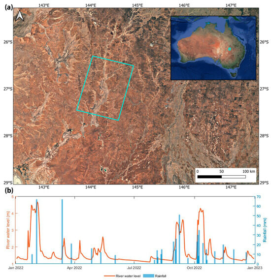
Figure 1.
(a) Study area is Quilpie, an arid region, located in southern Queensland, Australia (Imagery Source: Google Earth). (b) Rainfall and water levels from river gauge in Quilpie throughout 2022 [29,31].
Five datasets, collected by space-borne techniques and field surveys, were used to analyse erosion in the study area. These can be seen in Table 1.

Table 1.
The five datasets used in this study along with their product and usage.
SAR data were acquired from the Sentinel-1 mission, the product being L1 SLC in interferometric wide swath mode with VV polarisation. This polarisation was used as it often has a greater backscatter than VH, meaning it will provide better results for this study [32]. The data are provided by the European Space Agency via Copernicus Open Access Hub, with acquisition dates for each pair shown in Table 2 and Table S2. SAR data processing was carried out using SNAP software version 9.0.
Table 2.
The coherence pairs used in finding erosion, noting their dates and rainfall amounts.
Sentinel-2 data were used to calculate the Sentinel Water Index (SWI). These data were also provided by the European Space Agency via the Copernicus Open Access Hub. Sentinel-2 data have a spatial resolution of between 10 and 60 m, with the bands used in this study having a resolution of 20 m. Multispectral processing was also undertaken in SNAP. The Normalised Difference Vegetation Index (NDVI) was used to assess vegetation growth in the study area. NDVI was calculated using Sentinel-2 bands 4 (red) and 8 (NIR), giving it a resolution of 10 m. The Soil Moisture Active Passive (SMAP) mission by NASA was also used to identify changes in soil moisture. The L3_SM_P_E product was used, with a spatial resolution of 9 km, and was accessed through the Earth Data Hub.
A field campaign was conducted to collect the required field data for validation. A Phantom 4 RTK Drone with an RGB sensor and an RTK base station was used for imagery in pre-defined sections of the study area. The flights were completed at a height of 100 m, giving a ground sampling distance of 2.6 cm. There was a side and longitudinal overlap of 70%. The data were processed in Agisoft for mosaicking and geo-registration. Additionally, soil samples were collected from the study to test the sheer strength of the soils and their susceptibility to erosion [33].
2.2. Coherent Change Detection Method and Validation
The coherence pairs in Table 1 were calculated using the steps in Figure 2 and the parameters from Table 3. Firstly, the background coherence was established to identify erosion from the rain event. This was achieved by calculating the average and standard deviation (Figure 3) of seven coherence pairs (Table 1) that had little to no rainfall. These pairs will be referred to as the dry stack. The number of images used was such that it limited the computational requirements but still provided adequately accurate results. This was found through trial and error as it was found that the average and standard deviation did not change significantly when more than seven pairs were included in the process. The average percentage difference between using seven and eight pairs was 0.5% for the average and 1.6% for the standard deviation. This small change was seen as insignificant.
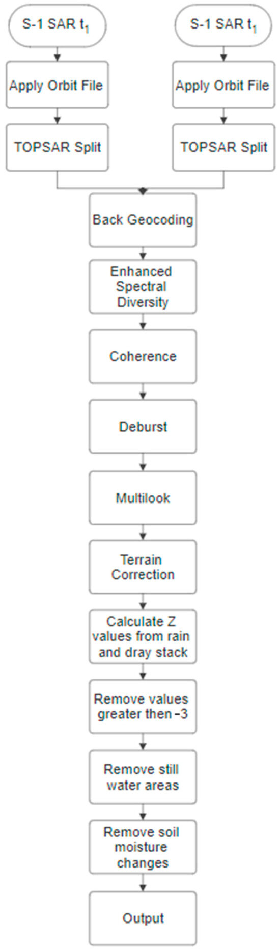
Figure 2.
The steps to create the erosion map.
Table 3.
Parameters used in the Sentinel Applications Program (SNAP) to calculate coherence values.
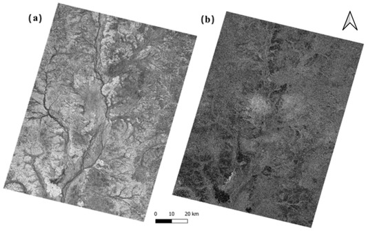
Figure 3.
(a) The average of the seven pairs with the brighter areas being closer to 1; (b) the standard deviation with whiter pixels representing a higher value.
The estimated average and standard deviations were then used to determine the Z-value for each pixel using Equation (3):
where is the -value, is the coherence value from the rain event, is the coherence mean from the dry stack, and is the standard deviation from the dry stack. This value represents the number of standard deviations the value from the rain event is away from the average value. To identify areas of erosion, any -values greater than −3 were removed. This means only values below −3 remained, which represents a 99% confidence interval. This 99% confidence interval was chosen through a process of trial and error using visual interpretation, with the 95% confidence interval leaving some artifacts visible in the data.
As water has a large effect on coherence values, the areas that have water on 7 February 2022 needed to be removed. Sentinel 2 data were used to calculate the Sentinel Water Index (SWI) to identify bodies of water [34]. The formula to calculate is shown below in Equation (4):
where is the vegetation red edge, which equates to band 5 and is the short-wave infrared, which equates to band 11.
This equation was used to create a binary map identifying bodies of water in the subject area on 7 February 2022. Any areas that had water were then removed from the erosion identification map. This binary map can be seen in Figure 4 and clearly shows that large sections of the area were inundated with water.
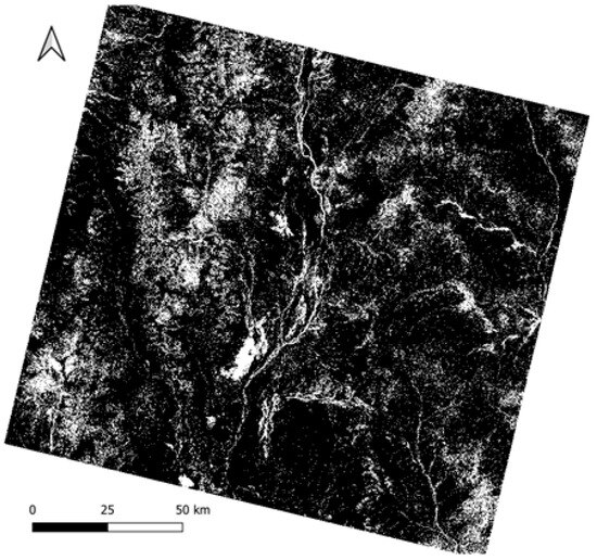
Figure 4.
Areas where water was lying on the 7 February 2022. The white pixels represent water while the black pixels are no water.
As soil moisture affects radar signals, any changes in soil moisture need to be mitigated. This was completed by using the same process as in Figure 2 but using the next coherence pair after the rain event, which was from 7 to 19 February 2022. As no rain occurred during this period, any areas highlighted should only be due to a loss of soil moisture or laying water. As such, any areas highlighted were removed from the erosion identification over the rain event. This correction may also remove some eroded areas but is necessary for removing false positives.
Due to the speckly nature of SAR data, small artefacts are present after completing the process above. These artefacts are only 1–4 pixels in size and obviously do not denote erosion but are more likely a result of the randomness in the one-coherence images from the rain event. Therefore, spatial filtering was applied to remove any pixel groups that were four pixels or less in size to achieve the final erosion identification map.
To validate this map, three different techniques were employed. These included assessing the effects of environmental factors, fieldwork using aerial photogrammetry, and temporal coherence variation. Details regarding these three techniques will be provided in the remainder of this section.
Using Equation (2), there are three environmental factors, namely geometric, volume, and thermal, that affect coherence and need to be controlled. These were each checked individually. To help assess the volumetric factors, coherence pairs with longer temporal baselines were produced. The pairs used can be seen in Table 4. This table shows the length of the temporal baselines and the rainfall amounts during these times.
Table 4.
The four coherence pairs used to analyse the effects of longer baselines on coherence.
Along with this, NDVI maps were created to assess any changes in vegetation over the course of the rain event. These were calculated using Formula (5).
where is the Normalised Difference Vegetation Index, is sentinel 2 band 8 or Near-infrared, and is sentinel 2 band 4.
Fieldwork was also completed to help validate the results. This first consisted of finding areas that likely contained erosion from the CCD analysis output. Suitable sites were chosen based on a few criteria including the density of pixels and localised increase in pixel values. Once a few suitable sites were selected, these areas were identified in the field and initial visual observations were undertaken. If obvious erosion could be identified visually, a drone flight was carried out. This consisted of using a Phantom 4 RTK Drone with the RTK base station. This drone survey was then compiled in Agisoft Metashape using a standard RTK process [35]. The ground control points (GCPs) measured by the field survey using a total station at each site were used to adjust the drone imagery. Testing determined that well-defined ground locations had an RMSE of 3 cm. In total, four drone flights were completed. The location of these flights and the other investigated areas are shown in Figure 5.
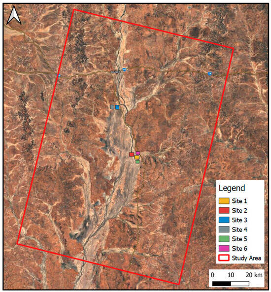
Figure 5.
The six sites investigated through the fieldwork were all situated south of Quilpie surrounding the Bulloo River.
In addition to the drone survey, soil samples from each site were also collected. Two samples from sites 1–4 were collected in soil sampling rings and stored in airtight containers. The location of each sample was chosen so that the sample would reflect the most prominent soil type of the area. In all test sites, the soil type found was Kandosol Red, a sandy surface soil with sandy-clay subsoils. A sheer strength test was completed on these samples to show the erodibility of the soils. This test was undertaken using the Shear Trak II by following the standards from AS1289.6.2.2 [36]. This standard outlines the correct methods and quality assurance to be used when testing the shear strength of soils. The results were then averaged between the two samples from each site, although only small differences were seen.
Lastly, temporal coherence variation was completed to help validate the erosion data. This consisted of finding the coherence of each 12-day pair over the entirety of 2022. This allowed for any variation in coherence to be examined over the course of the year. The SAR images used for this stage can be seen in Table S1 (Supplementary Materials). Using the same process as shown in Figure 2, coherence was calculated for each neighbouring pair, giving each coherence image a temporal baseline of 12 days. Next, five areas were chosen to be monitored, which consisted of three areas where erosion was identified, one control area with high coherence, and one control area with low coherence. The three eroded areas coincide with Site 1, Site 2, and Site 3 from Figure 5. Due to the aforementioned noisy nature of SAR images, a small area of 5000 m2 at each site was used to find the average value of the area. These data were then plotted with rainfall to show any relationship.
3. Results
This study clearly demonstrated widespread erosion around the river system as a result of the rain event on 2 February 2022 as shown in Figure 6. The speckly nature of SAR was evident in this image; however, it did suggest some areas of likely erosion. A number of these areas were then explored more in-depth during the field investigation.
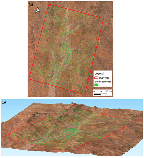
Figure 6.
(a)The erosion identification map after completing all corrections. Green pixels show where erosion was identified. (b) A 3D perspective of the subject area showing areas with identified erosion in green. Terrain was exaggerated to allow it to be seen.
As seen in Equation (2), there are four factors that contribute to coherence, being geometric, volumetric, thermal, and temporal. To ensure the results seen are only erosion, all other factors need to be removed. The geometric factors relate to changes in the physical position of the satellite between images. As stated earlier, pairs that have baselines larger than a few hundred metres may suffer from added decorrelation. The largest baseline in this study was 148 m as seen in Table S2 (Supplementary Materials). As such geometric factors should not be contributing towards coherence changes [25].
Next, the volumetric factors were explored. In this study, the most likely volumetric factors would be vegetation, soil moisture changes, and water. An assessment of the vegetation is shown in Figure 7. It can be seen there was only a small amount of vegetation change between the first and second SAR images. The most notable difference between the images occurs in the rivers where water is lying in the second image causing the pixels to become whiter. Normally, vegetation growth in arid and semi-arid environments tends to occur 1–2 months after rainfall [37,38]. As the temporal baseline between images is 12 days, the difference in vegetation cover should be relatively small. As such, vegetation should not create a difference in coherence.
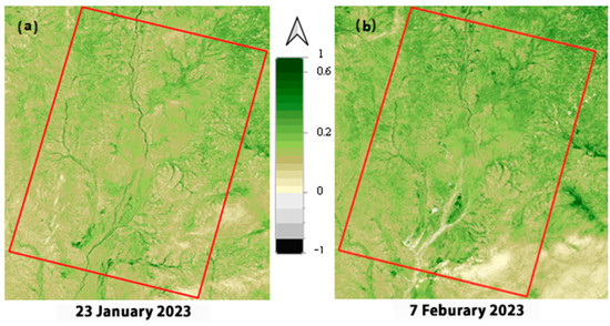
Figure 7.
NDVI from (a) before (23 January 2022) and (b) after (7 February 2022) the rain event on 2 February 2022. The greener a pixel, the denser the vegetation.
Soil moisture changes were examined in two ways, first using the Soil Moisture Active Passive (SMAP) mission and, secondly, using coherence pairs over longer temporal baselines. Figure 8 shows the difference between values gained from the SMAP mission L3_SM_P_E product on 27 January 2022 and 7 February 2022. This SMAP product has a spatial resolution of 9 km and, as such, can only be used to provide an approximate assessment of changes in soil moisture.
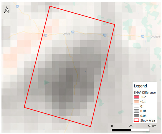
Figure 8.
Difference between the values gained from SMAP missions on 27 January 2022 and 7 February 2022. Positive values represent an increase in soil moisture.
As indicated in Figure 8, there has been a small increase in soil moisture; however, this increase is not considered significant. The SMAP mission has an accuracy of 0.04 m3/m3 [39], and as the largest difference in the study area is 0.053 m3/m3, it is only slightly higher than the accuracy of the equipment and, as such, is not considered a significant change.
To assess the moisture changes at a higher resolution, coherence pairs with different temporal baselines were investigated (Figure 9). If soil moisture was affecting the coherence signal, it would be expected that there would be an increase in coherence in some areas as soil moisture dissipated. This cannot be seen in Figure 9 as the coherence values decrease with time, with the average percentage difference between Figure 9a and d being −9.3%. This is what would normally be expected from longer temporal baselines. This same comparison was made in Figure 10 but over a dry period. Here, the average percentage difference was −5.2%, with a big portion begin concentrated in one area. This shows that there was a higher-than-normal decrease in coherence following the rain event, likely because of increased vegetation growth. This also shows that there were no increases in coherence due to soil moisture. Although these two data sources show that soil moisture should not have affected the study, soil moisture was still corrected as part of the method.
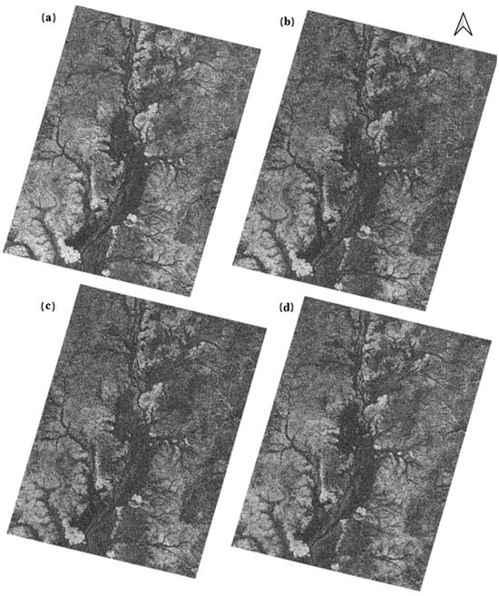
Figure 9.
The coherence over the subject area with different temporal baselines. The darker a pixel is, the lower the coherence. The baselines are (a) 12 days (26 January 2022–7 February 2022), (b) 24 days (26 January 2022–19 February 2022), (c) 36 days (26 January 2022–3 March 2022), and (d) 60 days (26 January 2022–27 March 2022).
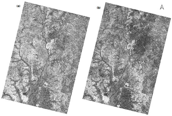
Figure 10.
The coherence over the area with longer baselines during a dry period. The darker a pixel the lower the coherence. The baselines are (a) 12 days (26 May 2022–7 June 2022) and (b) 60 days (26 May 2022–25 July 2022).
Lastly, laying water needs to be considered. Like most satellite data, SAR images cannot penetrate water bodies easily and, as such, in areas that may have still water, coherence values will be greatly affected. This factor was removed while processing as any areas with laying water were masked out.
The last factor to correct is the thermal factors. These factors are largely due to the limitations of the sensor, the atmospheric effects, and the randomness in any dataset [24]. Thermal factors cannot be easily corrected, so in this study, they have been limited by averaging pairs to create a dry stack and then utilising this stack to apply spatial filtering. These solutions do not totally remove all effects, as seen by the noisy nature of the final product. Through careful interpretation of the results, this factor did not contribute to large coherence changes. With all other factors largely removed from the dataset, it was assessed that the only remaining cause for coherence loss could be attributed to temporal factors. For this study, the possible temporal factors were all related to changes in the surface structure, either by natural or anthropogenic processes. Due to the remoteness of the study area, it can be assumed that direct anthropogenic effects would be very low. As such, it can be concluded that any effects seen in the final data are effects of natural processes. As there was a large amount of rainfall in the study area over the 12 days that covered these analyses, it can be assumed that most of the natural changes would be due to water erosion. However, in the data, some effects from wildlife are present.
The data collected from the field campaign can assist in interpreting the outcome of the SAR data processing. In total, six sites were visited, with four drone surveys and four soil samples being completed. These sites can be seen in Table 5 and are shown in Figure 5.
Table 5.
This table shows each of the sites visited along with a description of any erosion or site conditions seen.
Figure 11, Figures S1 and S2 show the four drone surveys with the erosion results overlayed. Some conclusions about the accuracy of the data can be drawn from these results; however, it is difficult with erosion to pinpoint newly eroded areas from past erosion. As erosion does not occur uniformly over a site, areas where erosion was determined in the images may not have eroded during the rain event on 2 February 2022. As such, these images can be used as a guide only to help validate the possible location of erosion.
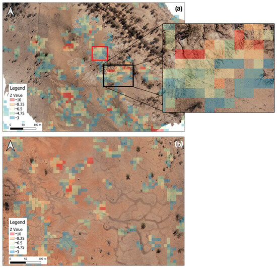
Figure 11.
Site 1 (a) and Site 4 (b) imagery from drone survey with erosion identification results. Pixel values represent the likelihood erosion occurred in that spot. Red box in (a) is area from Figure 12.
Figure 11a shows the results gained mostly coincide with erosion seen on the ground. Importantly, the data appears to suggest that erosion is occurring towards the end of the gullies, which is consistent with the natural formation of erosion. This is best seen in the detailed view in Figure 11a. The area contained within the red square can be seen in Figure 12. This area has obvious newly formed erosion.
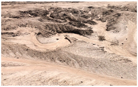
Figure 12.
Identified area of erosion from Site 1 showing the formation of new erosion. Photo: K Cook.
Figure 13 shows the two sites that were visited but no drone survey was undertaken. These sites were likely highlighted due to a combination of soil moisture changes and changes in the surface like flattened grass and disturbed rocks. It is obvious that little or no erosion had occurred in these areas largely due to their flatness. Water moving through this area would have a very low flow rate and, as such, would struggle to cause erosion. Figure 11b also highlights the need for continued improvement of this technique as it is obvious that some areas identified are likely soil moisture changes in the flat ground rather than erosion.
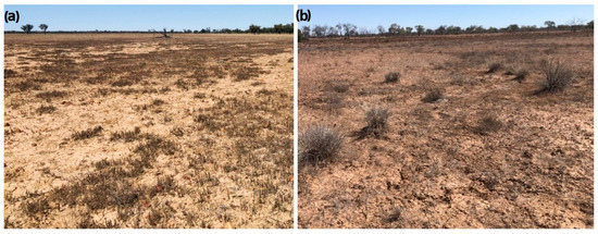
Figure 13.
Site 5 (a) and site 6 (b) where there are no significant signs of erosion but surface changes were likely. Photos: K Cook.
The shear strength of the soil from each of the drone flight areas can be seen in Table 6. Using the typical shear strength values from the GeotechniCal Reference Package by the University of West England, soft soil is rated as 20–40 kPa [40]. Each of the soil samples comfortably fit into this category, which is the second lowest possible strength category. This shows the weakness of these soils, which translates into a higher susceptibility to erosion [41].
Table 6.
The shear strength of soil samples taken from each of the drone survey sites.
In addition to the fieldwork, the temporal coherence variation was investigated as shown in Figure 14. Here, it can be seen that the coherence of five areas over the course of 2022 was plotted against rainfall data. Here Tests 1, 2, and 3 correspond to Sites 3, 2, and 1, respectively.
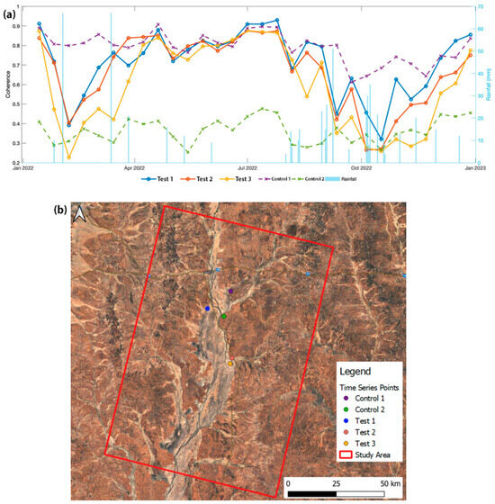
Figure 14.
(a) The temporal coherence variation of five areas shown on the map (b) can be seen throughout 2022 in the graph compared against rainfall. Coordinates for these points can be seen in Table S3 (Supplementary Materials).
It is evident from Figure 14 that there is a correlation between coherence and rainfall, although this correlation is not strong. Test areas 1, 2, and 3 had an average correlation coefficient of 0.61 while the control areas had a correlation of 0.24. However, this is to be expected as rainfall is not a perfect determinant of erosion. During the first rain event, all test areas where erosion is likely to have occurred saw a steep decrease in coherence, which resulted in high Z values, which can be seen in Table 4. This occurred while the two control areas remained largely unchanged. This same pattern occurs multiple times throughout the year.
It should be noted that even though Control 2 in Figure 14 was within a high coherence area, it did decrease throughout September to November 2022, likely due to changes in soil moisture; however, the decrease is small compared to that of the eroded areas. Another notable anomaly is the large rain event on 13 March 2022 that did not create a loss of coherence. This can be explained in two ways. By examining Figure 1b, during this rain event, the river levels were only slightly raised and did not reach the same heights as the 2 February rain event. Along with this, due to the large rain event that had occurred recently, any areas likely to easily erode would have already eroded. As such, experiencing lower erosion rates is expected. Figure 14 shows that coherence does appear to match erosion patterns over the course of 2022.
4. Discussion
The results presented from this model have identified areas that are likely to have eroded during the 2 February 2022 rain event. However, although the results are promising, further improvement is required to fully remove the effects of soil moisture. This study represents a new method for generating such results; a method that has advantages over similar studies. This study uses only seven coherence pairs to calculate the background coherence, resulting in significantly fewer computation resources than the SBAS method similar to Castellazzi et al. [28].
The approach utilised in this study used two vital corrections that had not been seen in previous studies, namely laying water and soil moisture corrections. The laying water correction was only required in areas that were prone to laying water such as in the channel country; however, the soil moisture correction is vital to all CCD analyses that revolve around rain. Castellazzi et al. [28] attempted to account for soil moisture using the stacking of coherence pairs with different temporal baselines; however, this did not completely explain how this removes soil moisture. As a result, the authors found that only 6 of the 13 identified areas could be attributed to erosion. Therefore, using a dedicated soil moisture correction like in this study may improve these results and are important to the validity of this study.
Even when considering the use of soil moisture removal, the largest impact on the accuracy of the erosion identification was the changes in soil moisture. Due to the flatness of the study area, many areas are inundated with water when rain occurs that then accumulates in the soil. When using soil moisture indices like SMAP or the Normalized Difference Moisture Index (NDMI), only small changes in soil moisture are evident. However, it appears that these small changes have a significant effect on the backscattered radar waves. Even when correcting for soil moisture changes seen in these indices, areas that do not seem to have erosion and likely have just experienced soil moisture changes are identified. This effect is not widespread, and with the knowledge of its existence, the data can be interpreted to determine the areas with actual erosion. Along with soil moisture, some other limitations exist, with these being the impacts of vegetation and the resolution of the mission. The lack of vegetation in the study area helped contribute to the strength of the results; however, in areas with higher vegetation, some artifacts existed. If this method were to be replicated in a highly vegetated area, it may struggle to identify erosion. This could be alleviated by using SAR satellites with longer wavelengths.
Additionally, the resolution of the Sentinel-1 SAR sensor means that some small amounts of erosion may not be detected in the large pixels. Identifying the implications of this factor is difficult due to two aspects. On the one hand, the effect of this factor is small as any changes to the surface structure do impact the intensity of the backscattered wave. On the other hand, small changes could be missed as they would be assumed to be noise. Even when considering these limitations, the method employed in this study is still widely usable.
Future studies should aim to better understand the effects of soil moisture on coherence values and attempt to find better ways for removing soil moisture content. This may be achieved using other sensors to measure soil moisture or by utilising a machine learning program to remove any defects. Such a process would create a more accurate representation of erosion.
5. Conclusions
Erosion is relentless, removing the precious resources of the land and leaving only scars behind. In doing so, it causes a loss in agricultural production, affects ecosystems, and disrupts waterways. Even with all these detrimental effects, the accurate and timely measurement of erosion continues to be challenging. This study aimed to contribute to knowledge on erosion by improving a method of locating erosion across large areas using a technique that was not computationally demanding. Data collected by the Sentinel-1 SAR mission throughout 2022 was used to determine erosion locations using coherence change detection, with other remotely sensed datasets being used to improve the erosion detection process. As a complementary analysis and to validate the results, a field campaign was also conducted. It was found that the method employed did locate erosion throughout the study area; however, it also showed false positives likely due to soil moisture changes. This study used a new method for removing soil moisture effects that did improve the accuracy of the data, but still left behind artefacts of soil moisture. Therefore, further minimisation of the soil moisture effects should be considered, but this study highlights the significant potential that an accurate and reliable erosion detection system could present.
Supplementary Materials
The following supporting information can be downloaded at: https://www.mdpi.com/article/10.3390/rs16071263/s1, Figure S1: Site 2 Imagery from drone survey with erosion identification results, Figure S2: Site 3 imagery from drone survey with erosion identification results, Table S1: SAR images used to assess the temporal coherence variation. It also states the spatial baseline of each image from the reference image, Table S2: SAR images used in finding erosion including their baseline distance from the reference image, Table S3: Coordinates of points used in the temporal coherence variation investigation (WGS 84 Zone 55S).
Author Contributions
Conceptualization, K.C.; methodology, K.C. and A.A.K.; software, K.C.; validation, K.C., A.A.K., A.G. and K.M.; formal analysis, K.C.; investigation, K.C., A.A.K. and K.M.; resources, K.M.; data curation, K.C.; writing—original draft preparation, K.C.; writing—review and editing, K.C., A.A.K., K.M. and A.G.; visualization, K.C. and A.A.K.; supervision, A.A.K.; project administration, A.A.K. All authors have read and agreed to the published version of the manuscript.
Funding
This research received no external funding.
Data Availability Statement
The Sentinel 1 SAR data used for finding eroded areas in this study were sourced from NASA’s EOSDIS via https://search.earthdata.nasa.gov/search?fst0=land%20surface (accessed on 2 February 2023) with a Creative Commons Zero license. The Sentinel 2 data used for generating NDVI and soil moisture in this study were sourced from NASA’s EOSDIS via https://search.earthdata.nasa.gov/search-?fst0=land%20surface (accessed on 10 July 2023) with a Creative Commons Zero license. The SMAP data used for monitoring soil moisture in this study were sourced from NASA’s EOSDIS via https://search.earthdata.nasa.gov/-search?fst0=land%20surface (accessed on 24 August 2023) with a Creative Commons Zero license. Version 9.0.0 of the Sentinel Application Platform (SNAP) was used to process all raw data, available at https://earth.esa.int/eogateway/tools/snap (accessed on 2 February 2023) with a GNU General Public License. Version 3.28.14 of QGIS was used to create figures, available at https://qgis.org/en/site/index.html (accessed on 2 February 2023) with a GNU General Public License.
Acknowledgments
The authors would also like to thank Nab Raj Subedi and Piumika Ariydasa for giving up their time to help complete the required tests.
Conflicts of Interest
The authors declare no conflicts of interest.
References
- Nearing, M.A.; Jetten, V.; Baffaut, C.; Cerdan, O.; Couturier, A.; Hernandez, M.; Le Bissonnais, Y.; Nichols, M.H.; Nunes, J.P.; Renschler, C.S.; et al. Modeling response of soil erosion and runoff to changes in precipitation and cover. CATENA 2005, 61, 131–154. [Google Scholar] [CrossRef]
- Teng, H.; Viscarra Rossel, R.A.; Shi, Z.; Behrens, T.; Chappell, A.; Bui, E. Assimilating satellite imagery and visible–near infrared spectroscopy to model and map soil loss by water erosion in Australia. Environ. Model. Softw. 2016, 77, 156–167. [Google Scholar] [CrossRef]
- Mathieu, D.B.; Wu, S.; Fredah, G.K. Economic analysis of the determinants of the adoption of water and soil conservation techniques in Burkina Faso: Case of cotton producers in the province of bam. J. Environ. Prot. 2019, 10, 1213–1223. [Google Scholar] [CrossRef]
- NSW Environmental Protection Authority. State of the Environment. 2003. Available online: https://www.epa.nsw.gov.au/about-us/publications-and-reports/state-of-the-environment/state-of-the-environment-2003 (accessed on 12 August 2023).
- Department of Agriculture Fisheries and Forestry. Agricultural Overview. Available online: https://www.agriculture.gov.au/abares/research-topics/agricultural-outlook/agriculture-overview (accessed on 1 April 2023).
- Bakker, M.M.; Govers, G.; Rounsevell, M.D. The crop productivity–erosion relationship: An analysis based on experimental work. Catena 2004, 57, 55–76. [Google Scholar] [CrossRef]
- Šarapatka, B.; Bednář, M. Agricultural Production on Erosion-Affected Land from the Perspective of Remote Sensing. Agronomy 2021, 11, 2216. [Google Scholar] [CrossRef]
- Zhang, L.; Huang, Y.; Rong, L.; Duan, X.; Zhang, R.; Li, Y.; Guan, J. Effect of soil erosion depth on crop yield based on topsoil removal method: A meta-analysis. Agron. Sustain. Dev. 2021, 41, 63. [Google Scholar] [CrossRef]
- USGS. Turbidity and Water. Available online: https://www.usgs.gov/special-topics/water-science-school/science/turbidity-and-water (accessed on 1 April 2023).
- Al-Kaisi, M.; Hanna, M.; Idman, M. Soil Erosion and Water Quality. Available online: https://crops.extension.iastate.edu/encyclopedia/soil-erosion-and-water-quality (accessed on 1 April 2023).
- Kingsford, R.; Dunn, H.; Love, D.; Nevill, J.; Stein, J.; Tait, J. Protecting Australia’s Rivers, Wetlands and Estuaries of High Conservation Value; Department of Environment and Heritage Australia: Canberra, Australia, 2005.
- Mulvihill, K. Soil Erosion 101. Available online: https://www.nrdc.org/stories/soil-erosion-101 (accessed on 18 April 2023).
- Agricultural Research Service. Revised Universal Soil Loss Equation (RUSLE)—Welcome to RUSLE 1 and RUSLE 2. Available online: https://www.ars.usda.gov/southeast-area/oxford-ms/national-sedimentation-laboratory/watershed-physical-processes-research/docs/revised-universal-soil-loss-equation-rusle-welcome-to-rusle-1-and-rusle-2/ (accessed on 17 March 2024).
- Pickup, G.; Chewings, V.H. A grazing gradient approach to land degradation assessment in arid areas from remotely-sensed data. Int. J. Remote Sens. 1994, 15, 597–617. [Google Scholar] [CrossRef]
- King, C.; Baghdadi, N.; Lecomte, V.; Cerdan, O. The application of remote-sensing data to monitoring and modelling of soil erosion. CATENA 2005, 62, 79–93. [Google Scholar] [CrossRef]
- de Jong, S.M.; Paracchini, M.L.; Bertolo, F.; Folving, S.; Megier, J.; de Roo, A.P.J. Regional assessment of soil erosion using the distributed model SEMMED and remotely sensed data. CATENA 1999, 37, 291–308. [Google Scholar] [CrossRef]
- Makaya, N.P.; Mutanga, O.; Kiala, Z.; Dube, T.; Seutloali, K.E. Assessing the potential of Sentinel-2 MSI sensor in detecting and mapping the spatial distribution of gullies in a communal grazing landscape. Phys. Chem. Earth Parts A/B/C 2019, 112, 66–74. [Google Scholar] [CrossRef]
- Vrieling, A. Mapping Erosion from Space; Wageningen University and Research: Wageningen, The Netherlands, 2007. [Google Scholar]
- Almagro, M.; Abrantes, N. Soil Water Erosion. Available online: https://climexhandbook.w.uib.no/2019/11/06/soil-water-erosion/ (accessed on 18 April 2023).
- Cabré, A.; Remy, D.; Aguilar, G.; Carretier, S.; Riquelme, R. Mapping rainstorm erosion associated with an individual storm from InSAR coherence loss validated by field evidence for the Atacama Desert. Earth Surf. Process. Landf. 2020, 45, 2091–2106. [Google Scholar] [CrossRef]
- Braun, A.; Veci, L. SAR Basics Tutorial. Available online: https://step.esa.int/docs/tutorials/S1TBX%20SAR%20Basics%20Tutorial.pdf (accessed on 19 April 2023).
- Xing, M.; Xing, M.; Lu, Z.; Yu, H. InSAR Signal and Data Processing; MDPI—Multidisciplinary Digital Publishing Institute: Basel, Switzerland, 2020. [Google Scholar]
- Zebker, H.A.; Villasenor, J. Decorrelation in interferometric radar echoes. IEEE Trans. Geosci. Remote Sens. 1992, 30, 950–959. [Google Scholar] [CrossRef]
- Jungkyo, J.; Duk-jin, K.; Lavalle, M.; Sang-Ho, Y. Coherent Change Detection Using InSAR Temporal Decorrelation Model: A Case Study for Volcanic Ash Detection. IEEE Trans. Geosci. Remote Sens. 2016, 54, 5765–5775. [Google Scholar] [CrossRef]
- Meng, W.; Sandwell, D.T. Decorrelation of L-Band and C-Band Interferometry Over Vegetated Areas in California. IEEE Trans. Geosci. Remote Sens. 2010, 48, 2942–2952. [Google Scholar] [CrossRef]
- Gatelli, F.; Guamieri, A.M.; Parizzi, F.; Pasquali, P.; Prati, C.; Rocca, F. The wavenumber shift in SAR interferometry. IEEE Trans. Geosci. Remote Sens. 1994, 32, 855–865. [Google Scholar] [CrossRef]
- Schepanski, K.; Wright, T.; Knippertz, P. Evidence for flash floods over deserts from loss of coherence in InSAR imagery. J. Geophys. Res. Atmos. 2012, 117, D20101. [Google Scholar] [CrossRef]
- Castellazzi, P.; Khan, S.; Walker, S.J.; Bartley, R.; Wilkinson, S.N.; Normand, J.C.L. Monitoring erosion in tropical savannas from C-band radar coherence. Remote Sens. Environ. 2023, 290, 113546. [Google Scholar] [CrossRef]
- Bureau of Meteorology. Quilpie Climate Data. Available online: http://www.bom.gov.au/jsp/ncc/cdio/weatherData/av?p_nccObsCode=139&p_display_type=dataFile&p_startYear=&p_c=&p_stn_num=045015 (accessed on 27 August 2023).
- FitzSimons, T. Channel Country. Available online: https://www.qhatlas.com.au/content/channel-country (accessed on 27 August 2023).
- Queensland Government. Bulloo River at Quilpie. Available online: https://water-monitoring.information.qld.gov.au?ppbm=011203A&rs&1&rslf_org (accessed on 4 March 2023).
- Quang, N.; Quinn, C.; Stringer, L.; Carrie, R.; Hackney, C.; Huế, L.; Dao, T.; Pham, N. Multi-Decadal Changes in Mangrove Extent, Age and Species in the Red River Estuaries of Viet Nam. Remote Sens. 2020, 12, 2289. [Google Scholar] [CrossRef]
- Bishop, A.W. The Strength of Soils as Engineering Materials. Géotechnique 1966, 16, 91–130. [Google Scholar] [CrossRef]
- Jiang, W.; Ni, Y.; Pang, Z.; Li, X.; Ju, H.; He, G.; Lv, J.; Yang, K.; Fu, J.; Qin, X. An Effective Water Body Extraction Method with New Water Index for Sentinel-2 Imagery. Water 2021, 13, 1647. [Google Scholar] [CrossRef]
- Agisoft. Agisoft Metashape User Manual Professional Edition. Available online: https://www.agisoft.com/pdf/metashape-pro_2_0_en.pdf (accessed on 19 October 2023).
- Standards Australia. AS 1289.6.2.2:2020; Standard Australia: Sydney, NSW, Australia, 2020; Volume 2, p. 17. [Google Scholar]
- Wu, T.; Bai, H.; Feng, F.; Lin, Q. Multi-month time-lag effects of regional vegetation responses to precipitation in arid and semi-arid grassland: A case study of Hulunbuir, Inner Mongolia. Nat. Resour. Model. 2022, 35, e12342. [Google Scholar] [CrossRef]
- Schmidt, H.; Karnieli, A. Remote sensing of the seasonal variability of vegetation in a semi-arid environment. J. Arid. Environ. 2000, 45, 43–59. [Google Scholar] [CrossRef]
- NASA. SMAP Specifications. Available online: https://smap.jpl.nasa.gov/observatory/specifications/#:~:text=With%20this%20great%20difference%20between,temperature’%20of%20the%20land%20surface (accessed on 28 August 2023).
- Davison, D.L. Basic Mechanics of Soils. Available online: http://environment.uwe.ac.uk/geocal/soilmech/basic/soilbasi.htm (accessed on 31 August 2023).
- Léonard, J.; Richard, G. Estimation of runoff critical shear stress for soil erosion from soil shear strength. CATENA 2004, 57, 233–249. [Google Scholar] [CrossRef]
Disclaimer/Publisher’s Note: The statements, opinions and data contained in all publications are solely those of the individual author(s) and contributor(s) and not of MDPI and/or the editor(s). MDPI and/or the editor(s) disclaim responsibility for any injury to people or property resulting from any ideas, methods, instructions or products referred to in the content. |
© 2024 by the authors. Licensee MDPI, Basel, Switzerland. This article is an open access article distributed under the terms and conditions of the Creative Commons Attribution (CC BY) license (https://creativecommons.org/licenses/by/4.0/).