Spectral-Spatial-Sensorial Attention Network with Controllable Factors for Hyperspectral Image Classification

Abstract

Hyperspectral image (HSI) classification aims to recognize categories of objects based on spectral–spatial features and has been used in a wide range of real-world application areas. Attention mechanisms are widely used in HSI classification for their ability to focus on important information in images automatically. However, due to the approximate spectral–spatial features in HSI, mainstream attention mechanisms are difficult to accurately distinguish the small difference, which limits the classification accuracy. To overcome this problem, a spectral–spatial-sensorial attention network (S³AN) with controllable factors is proposed to efficiently recognize different objects. Specifically, two controllable factors, dynamic exponential pooling (DE-Pooling) and adaptive convolution (Adapt-Conv), are designed to enlarge the difference in approximate features and enhance the attention weight interaction. Then, attention mechanisms with controllable factors are utilized to build the redundancy reduction module (RRM), feature learning module (FLM), and label prediction module (LPM) to process HSI spectral–spatial features. The RRM utilizes the spectral attention mechanism to select representative band combinations, and the FLM introduces the spatial attention mechanism to highlight important objects. Furthermore, the sensorial attention mechanism extracts location and category information in a pseudo label to guide the LPM for label prediction and avoid details from being ignored. Experimental results on three public HSI datasets show that the proposed method is able to accurately recognize different objects with an overall accuracy (OA) of 98.69%, 98.89%, and 97.56%, respectively.

1. Introduction

A hyperspectral image (HSI) is a three-dimensional cube composed of spectral and spatial information. Among them, the spectral information consists of hundreds of continuous narrow bands that record the reflectance values of light from visible to infrared [1]. The spatial information consists of pixels that describe the distribution of land cover [2]. The abundant spectral and spatial information improves the reliability and stability of object analysis [3]. Therefore, the interpretation of HSI is widely used in precision agriculture, land management, and environmental monitoring [4].

HSI classification attempts to assign labels for each pixel and obtains the category of different objects [5]. In the early stages, some classical machine learning models were proposed for HSI classification, such as k-means clustering [6], multinomial logistic regression (MLR) [7], random forest (RF) [8], and support vector machine (SVM) [9], et al., which extract the representative features and assign the categories with sufficient labeled samples [10]. However, these models are difficult to capture the correlation of spectral and spatial information and to distinguish the approximate features.

Deep learning models apply neural networks to automatically extract local and global features, and fully consider the contextual semantics to obtain the abstract representation of spectral–spatial features [11]. As the commonly used model, the convolutional neural network (CNN), with the characteristics of local connection and weight sharing, extracts spectral–spatial features simultaneously [12]. 2D-CNN and 3D-CNN are used in HybridSN to capture the semantic features of the HSI patches [13]. However, adjacent patch samples contain a large overlapping area, which entails expensive computational costs [14]. To reduce the overlapping computation, spectral–spatial residual networks (SSRN) [15], spectral–spatial fully convolutional networks (SSFCN) [16], and fast patch-free global learning (FPGA) [17] were proposed to take HSI cubes or entire images as training samples and upgrade pixel-to-pixel classification to image-to-image classification. The deep learning models utilize convolutional layers to expand the receptive field, andextract the correlation of long-range features to improve the classification accuracy [18]. However, these models face the problem of detail loss during feature extraction, i.e., the details within a few pixels gradually decrease and are likely to disappear after several down-sampling.

To retain detailed features that provide sufficient information for label prediction, attention mechanisms have attracted widespread interest for their ability to emphasize important objects, which are like the eye of models, automatically capturing the important objects and ignoring the background, and the capability of feature extraction is significantly improved with a small computation sacrifice [19]. In addition, the pooling operation and multilayer perceptron (MLP) are utilized to quickly evaluate the importance of features and assign the corresponding weights [20]. Some classical attention mechanisms, such as “squeeze and excitation” (SE) [21], convolutional block attention module (CBAM) [22], and efficient channel attention (ECA) [23], measure the importance of spectral and spatial features with weights, as well as delineate the attention regions. However, the pooling operation is difficult to distinguish the continuous and approximate features of HSI, and results in inaccurate attention regions, which is described as “attention escape”.

The inaccurate attention region is mainly caused by the imprecise evaluation of attention weights, and adjusting the evaluation manner could effectively mitigate this problem [24]. Therefore, controllable factors are introduced to enlarge the differences in approximate features and enhance the sensitivity of attention mechanisms [25]. For example, the deep square pooling operation was proposed to increase the difference in continuous features by using pixel-wise squares to generate more discriminative weights [26]. The coordinate attention mechanism (CAM) was proposed to locate important objects to efficiently capture the long-range dependency of features [27]. The residual attention mechanism (RAM) introduced residual branches to fuse shallow features and control the spatial semantics padding of trunk branches [28]. These approaches adjust the evaluation manner of attention mechanisms and obtain more accurate attention weights to emphasize the important objects [29]. However, controllable factors lack the dynamic adjustment ability to adapt to the complex and continuous feature environment of HSI.

In this paper, a spectral-spatial-sensorial attention network (S³AN) with controllable factors is proposed for HSI classification. In S³AN, attention mechanisms and convolutional layers are encapsulated in the redundancy reduction module (RRM), feature learning module (FLM), and label prediction module (LPM). Specifically, dynamic exponential pooling (DE-Pooling) and adaptive convolution (Adapt-Conv), as controllable factors, participate in weight sharing and convey information via interfaces to balance the control effect of modules. In RRM, the spectral attention mechanism converts the spectral features into band weights, evaluates them by reconstructive convolution (Rec-Conv), and selects important bands to construct dimension-reduced features. In FLM, the spatial attention mechanism with double branches is utilized to pad details and emphasize spatial features, and cross-level feature learning (CFL) is utilized to extract the abstract representation of deep and shallow features. In LPM, the sensorial attention mechanism is utilized to search for the coordinates of labeled pixels and guides transition convolution (Trans-Conv) for pixel-wise classification. Finally, a lateral connection is used to fuse the three functional modules, gradually optimizing the representation of features and improving the classification accuracy. The main contributions of this paper are listed as follows:

• A S³AN with controllable factors is proposed for HSI classification. The S³AN integrates redundancy reduction, feature learning, and label prediction processes based on the spectral-spatial-sensorial attention mechanism, which refines the transformation of features and improves the adaptability of attention mechanisms in HSI classification;
• Two controllable factors, DE-Pooling and Adapt-Conv are developed to balance the differences in spectral–spatial features. The controllable factors are dynamically adjusted through backpropagation to accurately distinguish continuous and approximate features, and improve the sensitivity of attention mechanisms;
• A new sensorial attention mechanism is designed to enhance the representation of detailed features. The category information in the pseudo label is transformed into the sensorial attention map to highlight important objects, and position details and improve the reliability of label prediction.

2. Related Work and Motivations

HSI classification, as a pixel-wise classification task, relies on the contextual semantic extraction of spectral–spatial features [30]. To improve classification accuracy, CNN and attention mechanisms have attracted widespread interest for their ability to extract contextual semantics and emphasize important objects.

2.1. HSI Classification Based on CNN

The CNN-based methods utilize convolutional layers to automatically extract spectral–spatial features to implement end-to-end HSI classification and achieve satisfactory performance [31]. A Conv-Deconv network (CDN) was proposed for HSI classification, which integrated feature extraction and feature recovery processes based on encoder-decoder structure for unsupervised spectral–spatial feature learning [32]. To avoid overfitting, SSRN proposed a spectral–spatial residual network to take 3D cubes as training samples, which avoids complex feature engineering of HSI [15]. To reduce the complexity of the model, HybridSN fused 3D-CNN and 2D-CNN to analyze the correlation of spatial and spectral information and obtain a more abstract level of spatial representation [13]. Dynamic low-rank and sparse priors constrained deep autoencoders (DLRSPs-DAEs) fully utilized the low-rank and sparse property of HSI, and combined the low-rank sparse model (LRSM) with deep auto-encoder (DAE) to capture the important features of HSI [33]. Further, fast patch-free global learning (FPGA) was proposed for HSI classification, which was based on a global stochastic stratified (GS²) sampling strategy and FreeNet to achieve an end-to-end classification of the entire image [17]. However, these methods ignore the dimensional mutation problem in the prediction layer, i.e., the semantic feature map is suddenly transformed into the classification result that is the same size as the original image. During up-sampling, the feature map is padded with many irrelevant elements, which corresponds to increased noise and even suppresses the representation of details [34].

2.2. HSI Classification Based on Attention Mechanism

The attention mechanism-based methods highlight the important spectral–spatial features and play an active assistance role in HSI classification [35]. Double-branch multi-attention network (DBMA) constructed a branching framework based on the spectral attention mechanism and spatial attention mechanism to extract 3D cube features simultaneously [36]. To boost the interaction of features, the residual spectral–spatial network (RSSN) introduced residual blocks in the spatial and spectral network, and combined them with contextual semantics to optimize the representation of features [37]. Spectral–spatial attention networks (SSAN) embedded the attention mechanism into RNN and CNN, respectively, thus achieving a sufficient learning of continuous spectral information and the spatial correlation of adjacent pixels [38]. Deep self-representation learning framework (DLSF) adaptively removed anomalous pixels from HSI by an alternating optimization strategy, and introduced a subspace recovery autoencoder (SRAE) to sense the local anomalous pixels by using spatial detail information [39]. In addition, the band selection methods that contained spectral attention mechanisms, such as BS-Net [40] and TAttRecNet [41], also became popular for HSI processing. However, the attention mechanism in these methods is insensitive to the difference in approximate features, which affects the generation of attention weights and limits the final classification accuracy.

2.3. Motivations

Since some CNN-based HSI classification methods tend to ignore detail features during down-sampling, which makes it difficult for details to provide knowledge for label prediction [42]. To address this problem, a spatial attention mechanism with double branches is applied to pad shallow features; skip connections are introduced in CFL to interact with deep and shallow features; a sensorial attention mechanism and Trans-Conv are added to emphasize the important objects and retain sufficient details for label prediction.

The inaccurate evaluation manner decreases the sensitivity of attention mechanisms, and results in difficulty in generating clear category boundaries for attention mechanism-based HSI classification methods [43]. To address this problem, controllable factors are introduced to dynamically adjust the differences in spectral–spatial features. Among them, DE-Pooling is utilized to enlarge the differences in approximate features to obtain more distinguishable feature weights. Adapt-Conv is utilized to enhance the interaction efficiency of feature weights and capture the correlation of adjacent and long-range features. The main purpose of controllable factors is to improve the sensitivity of attention mechanisms to generate accurate attention regions.

Hence, S³AN integrates RMM, FLM, and LPM for redundancy reduction, feature learning, and label prediction, respectively. The controllable factors, DE-Pooling and Adapt-Conv, are utilized to adjust the delineation of attention regions and update the control effect by the backpropagation to balance the feature extraction ability. RRM combines spectral attention mechanism and Rec-Conv to select important bands for the construction of dimension-reduced features, and reduces the computational cost of feature learning. FLM fuses spatial attention mechanism and CFL to extract spectral–spatial contextual semantics and learn the abstract representation of features. In addition, LPM attempts to introduce the sensorial attention mechanism and Trans-Conv to mitigate dimensional mutation to improve the final classification accuracy.

3. Materials and Methods

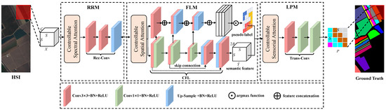
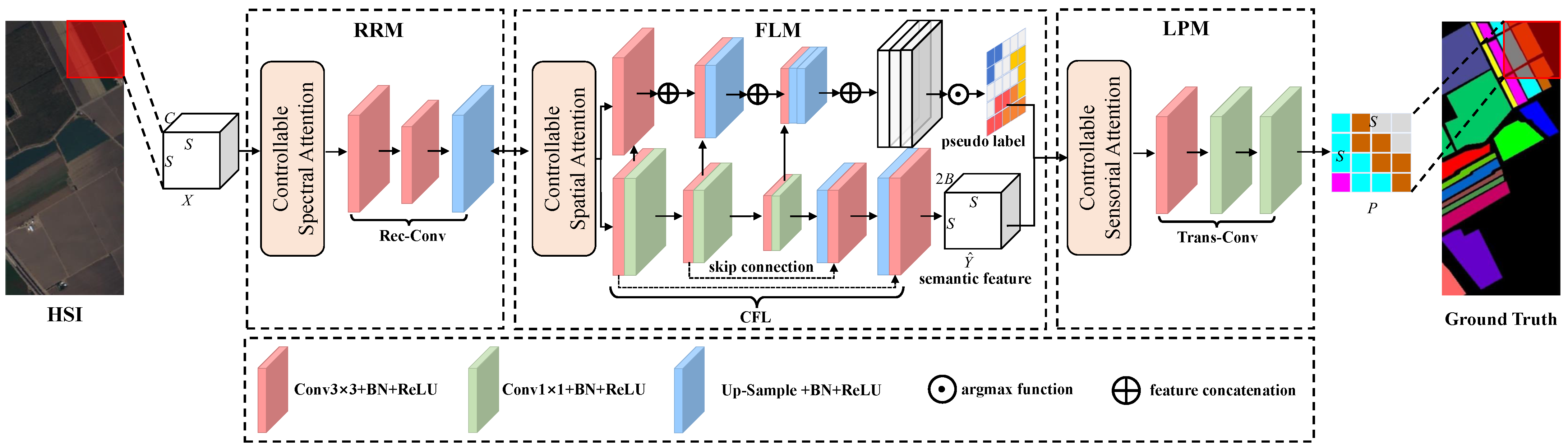
S³AN designs functional modules based on attention mechanisms and convolutional layers, where the attention mechanism reweights feature maps to generate feature masks, and combines with convolution layers to extract abstract representation. A lateral connection is utilized to integrate these modules and interfaces are applied to convey feature maps and feedback information. As shown in Figure 1, the HSI cube is defined as $X\in R^{C\times S\times S}$, where S and C are the input size and the number of bands, respectively. The original image is transformed by RRM, the spectral feature is converted into a weight vector by spectral attention mechanism; Rec-Conv is utilized to update the weights; and the top B bands with the highest weights are selected to construct the dimension-reduced feature that replaces the original image. Then, the dimension-reduced feature is delivered to FLM via the interface, and the spatial attention mechanism is applied to pad some shallow details; the spectral–spatial contextual semantic features are extracted by CFL, and the pseudo label is created through multi-scale feature fusion. Further, the pseudo label is transformed into a sensorial attention map by the sensorial attention mechanism, and Trans-Conv is guided to focus on the labeled pixels to optimize the representation of semantic features. Finally, the classification result is obtained by LPM.

Figure 1. The overall architecture of S³AN. S³AN is mainly divided into three modules, i.e., RRM, FLM, and LPM. RRM selects important bands for redundancy reduction; FLM extracts contextual semantics for feature learning; LPM positions global objects for label prediction.

3.1. Controllable Factors

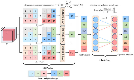
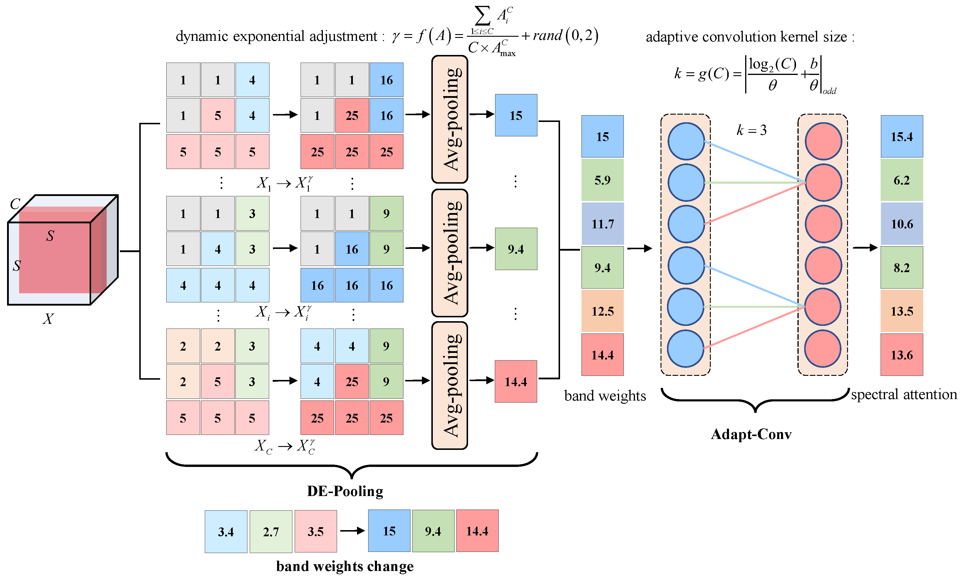
To improve the ability of attention mechanisms to distinguish approximate spectral–spatial features, two controllable factors are proposed; that is, dynamic exponential pooling (DE-Pooling) and adaptive convolution (Adapt-Conv), and the detailed structure is shown in Figure 2.

Figure 2. The details of controllable factors. DE-Pooling balances the differences in approximate features, Adapt-Conv enhances the interaction efficiency of feature weights.

3.1.1. DE-Pooling

DE-Pooling adds a dynamic exponent computation before the global average pooling to control the fluctuation of spectral–spatial features [44]. As shown in Figure 2, taking the DE-Pooling of spectral feature as an example, the HSI cube is split into hundreds of bands, and then each band $X_i$ is enlarged by an exponential multiple. This enlargement process highlights the differences in information between adjacent bands, making each band independently weighted. As seen in the band weights change, the approximate feature becomes more distinguishable. To adjust the spectral feature within a suitable range, the dynamic exponent is adjusted based on spectral attention weights, and the adjustment process is written as

$$\gamma =f\left(A\right)=\frac{{\sum }_{i=1}^C{A}_i^C}{C\times A_{max}^C}+rand\left(0,2\right)$$

(1)

where $f\left(A\right)$ denotes the mapping of dynamic exponent to spectral attention weights, $A_i^C$ denotes the i-th spectral attention weight, and $A_{max}^C$ denotes the maximum spectral attention weight. In addition, the original physical properties of HSI spectral–spatial features are altered as the dynamic exponent $\gamma$ continues to increase. Therefore, to avoid the infinite enlargement of the spectral features, expecting the feature value x to change within the interval $(x,x^3)$, $rand\left(0,2\right)$ is added to limit the variation in the dynamic exponent.

3.1.2. Adapt-Conv

To relate local and global features and improve the interaction efficiency of band weights, Adapt-Conv utilizes 1D-convolution instead of MLP and sets an adaptive convolutional kernel to control the information interaction range [45]. Adapt-Conv for band weight interaction is shown in Figure 2, where the adaptive convolutional kernel size is set to 3. To achieve adaptive adjustment of the kernel size, the mapping is conducted to describe the relationship between the number of bands and the kernel size. Considering that there may also be a positive proportional mapping between the number of bands and the kernel size, the mapping is written as

$$C=2^{\left(\theta \times k+b\right)}$$

(2)

where the kernel size k, $\theta$ and b are controllable parameters. Since the number of bands C is usually close to being a power of 2, the mapping relation is defined as a nonlinear function $2^{\left(\theta \times k+b\right)}$. Thus, after a given number of bands C, the kernel size k is calculated using the inverse function, which is written as

$$k=g\left(C\right)={\left|\frac{lo{g}_2\left(C\right)}{\theta }+\frac{b}{\theta }\right|}_{odd}$$

(3)

where $g\left(C\right)$ denotes the mapping of the kernel size k to the number of bands C. Since the convolutional kernel slides with the center as an anchor point, whereas odd convolutional kernel has a natural center point. Therefore, the odd operation ${\left|t\right|}_{odd}$ is set in Adapt-Conv, and it is taken as an odd number close to t.

3.2. Redundancy Reduction Module (RRM)

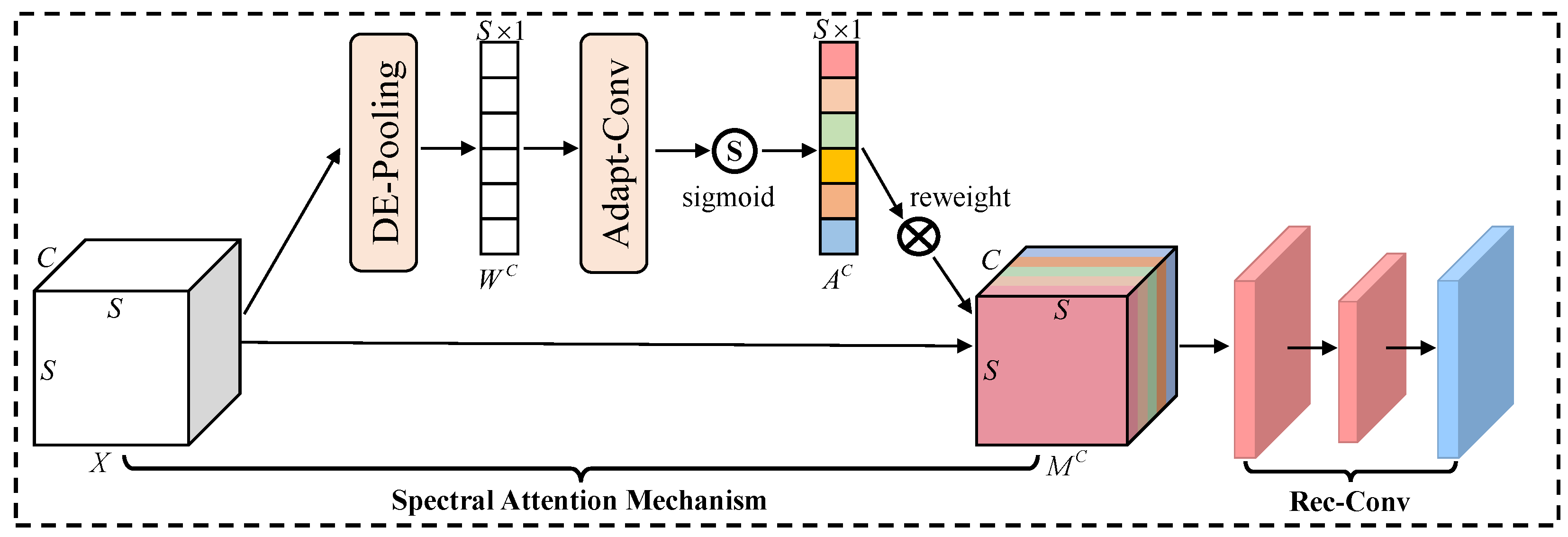
RRM converts the reduction in spectral redundancy to a band reconstruction task, i.e., recovering the complete image with a few important bands [40]. Therefore, the band importance is evaluated by the spectral attention mechanism, and the spectral attention weights are updated by Rec-Conv, selecting the bands that are essential for spectral reconstruction to construct the dimension-reduced feature.

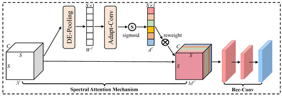
As shown in Figure 3, the HSI cube X is fed into the spectral attention mechanism, and DE-Pooling fully considers the difference in spectral features and assigns a unique band weight $w_i$ to each band. Further, the band weights $W^C$ are conveyed to Adapt-Conv for local and global features interaction and obtain the final spectral attention map $A^C$. Therefore, the generation of the spectral attention map is written as

$$A^C=\sigma \left(Adap{t}_{conv}\left(D{E}_{pool}\left(X\right)\right)\right)$$

(4)

where $\sigma$ is the sigmoid activation function, $Adap{t}_{conv}$ denotes the adaptive convolution, and $D{E}_{pool}$ denotes the dynamic exponential pooling. Furthermore, a band-wise multiplication operation is applied to create the interaction between the HSI cube and the spectral attention map to obtain the spectral feature mask $M^C=X\otimes A^C$.

Figure 3. The details of RRM, where X denotes the HSI cubes, $W^C$ denotes the band weights, $A^C$ denotes the spectral attention map, and $M^C$ denotes the spectral feature mask.

Rec-Conv aims to improve the weights of important bands and suppress the representation of redundant bands. This structure consists of two $Conv3\times 3$ and a nearest interpolation function for recovering the spectral feature mask. Then, calculate the loss between the original and recovered images, and update the band weights. After several iterations, the important bands will obtain the higher weight. Finally, the top B bands with the highest weights are selected by sorting, and their indexes are conveyed to FLM.

3.3. Feature Learning Module (FLM)

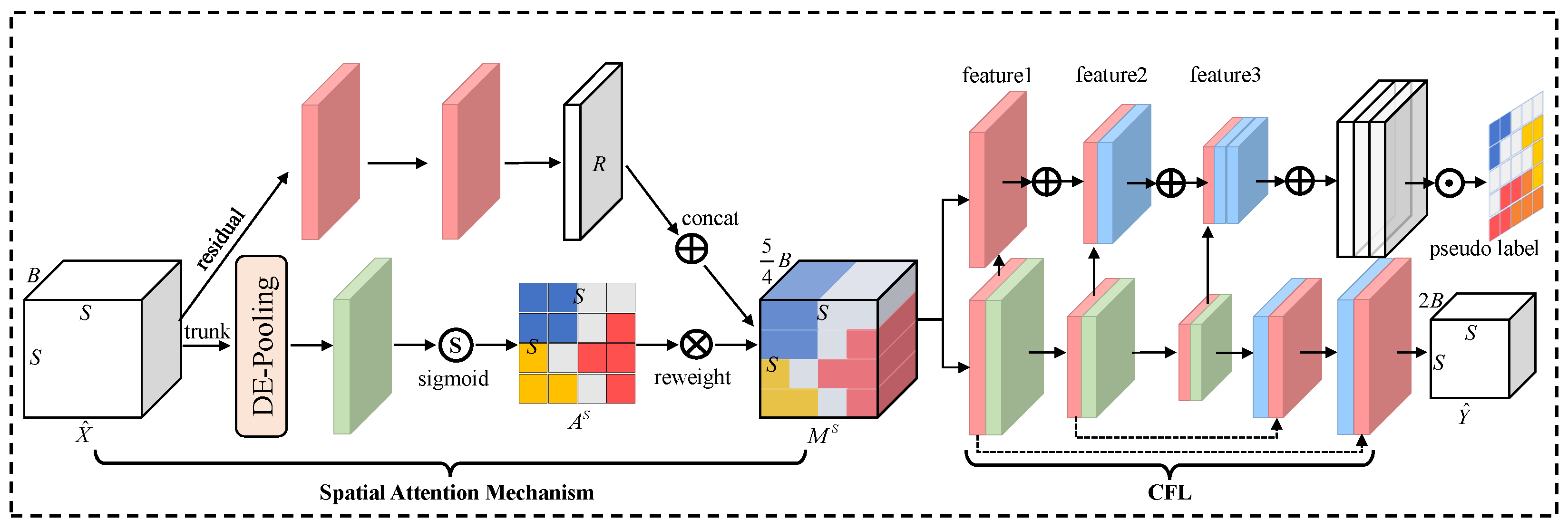
In FLM, the spatial attention mechanism emphasizes global spatial features by the trunk branch and pads the details by the residual branch. Then, CFL is applied to extract the contextual semantics by skip connection and multi-scale feature fusion.

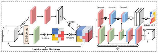
As shown in Figure 4, the dimension-reduced feature $\widehat{X}\in R^{B\times S\times S}$ is received by the spatial attention mechanism and allocated to two branches for processing. In the trunk branch, DE-Pooling is utilized to balance the difference in spatial features and assign spatial attention weights to each pixel. Then, the spatial information interaction is performed by a $Conv1\times 1+BN+ReLU$ convolutional combination, and obtain the spatial attention map $A^S$. In the residual branch, the input feature $\widehat{X}$ is fed into two convolution combinations of $Conv3\times 3+BN+ReLU$ to extract a shallow feature map $R\in R^{\frac{B}{4}\times S\times S}$. Therefore, the generation of the spatial attention map is written as

$$A^S=\sigma \left(F^{1\times 1}\left[D{E}_{pool}\left(\widehat{X}\right)\right]\right)$$

(5)

where $F^{1\times 1}$ denotes a convolution operation with a filter size of $1\times 1$. The pixel-wise multiplication operation is applied to create the interaction of spatial attention map and dimension-reduced feature to obtain the trunk feature mask $T\in \widehat{X}\otimes A^S$. Further, the trunk feature mask T and the shallow feature map R are concatenated by weighted fusion to obtain a spatial feature mask $M^S=T+\lambda R$.

Figure 4. The details of FLM, where $\widehat{X}$ denotes the dimension-reduced feature, $A^S$ denotes the spatial attention map, $M^S$ denotes the spatial feature mask, and $\widehat{Y}$ denotes the semantic feature map.

CFL following the encoder-decoder structure is mainly applied to extract contextual semantics. Among them, the encoder utilizes several $Conv3\times 3+BN+ReLU$ convolutional combinations for down-sampling and feature learning to obtain abundant semantic information. The decoder utilizes several nearest interpolation functions for up-sampling and spatial feature recovery to obtain the semantic feature map that is of the same size as the original image.

Furthermore, the pseudo label is generated by multi-scale feature fusion. The shallow feature map (feature1) and deep feature maps (feature2, feature3) extracted by the encoder are selected for feature concatenation. Since the size of the deep feature maps are 1/2 and 1/4 of the input image, respectively, and not directly usable for creating the pseudo label. Therefore, two nearest neighbor interpolation functions are used to recover the size of the deep feature maps, when the feature maps are of uniform size, they are then concatenated by using the $concat$ operation. In this way, the obtained feature maps with object locations that are similar to the input image. Further, the argmax function value is computed to obtain the possible category information in each pixel. In general, the pseudo label is an advanced prediction result that provides the location and category information of ground objects.

3.4. Label Prediction Module (LPM)

In LPM, the sensorial attention mechanism is applied to search for the labeled pixels in the semantic feature map, and Trans-Conv is applied to transition the semantic feature map into the classification result. Therefore, the module improves the stability and reliability of label prediction by object position and feature transition.

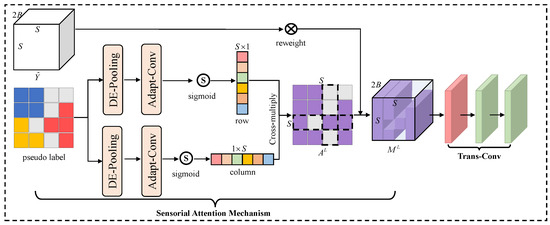
As shown in Figure 5, the sensorial attention mechanism extracts the location and category information in the pseudo label and guides the model to focus on the location where objects are likely to be present, so that important details are not ignored by the model. Specifically, the pseudo label is fed to the sensorial attention mechanism, and its row and column elements are extracted by using DE-Pooling and Adapt-Conv. Then, the row and column sensorial attention weights are cross-multiplied to generate the complete sensorial attention map $A^L$. Thus, the generation of the sensorial attention map is written as

$$A^L=\sigma \left(Adap{t}_{conv}\left(D{E}_{pool}\left(Row\right)\right)\times Adap{t}_{conv}\left(D{E}_{pool}\left(Column\right)\right)\right)$$

(6)

where $Row$ and $Column$ indicate the row and column elements of the pseudo label, respectively. Then, a pixel-wise multiplication operation is applied to create the interaction of the sensorial attention map and the semantic feature map $\widehat{Y}$ to obtain the sensorial feature mask $M^L=\widehat{Y}\otimes A^L$.

Figure 5. The details of LPM, where $row$ denotes the row sensorial attention weights, $column$ denotes the column sensorial attention weights, $A^L$ denotes the sensorial attention map, and $M^L$ denotes the sensorial feature mask.

Trans-Conv is applied to mitigate the dimensional mutation in the prediction layer and has a flexible design concept. Its depth is determined by the size of the semantic feature map $\widehat{Y}$ and the dimensional reduction coefficient r. The appropriate Trans-Conv layers both increase the model depth and retain details for label prediction. Therefore, the mapping of the Trans-Conv layers l and the semantic feature dimension D is established as

$$l=\frac{1}{2}\left|lo{g}_r\left(D-class\right)\right|$$

(7)

where r denotes the dimensional reduction coefficient. Since the number of channels of the semantic feature map is reduced to $class$, so the dimensional distance is $D-class$. Finally, the output of Trans-Conv is performed for label prediction to obtain the classification result P.

3.5. S³AN for HSI Classification

To meet the requirements of HSI classification, S³AN designs RRM, FLM, and LPM based on attention mechanisms with controllable factors to process the original image. Among them, controllable factors and detail processing approaches are utilized to address the problems of “attention escape” and detail loss. A lateral connection is applied to integrate three functional modules, and the interfaces are used to convey feature maps and feedback information between the modules. Therefore, the original image X is transformed by these modules to obtain the classification result P. To train the model and adjust the controllable factors, the cross-entropy is utilized as the loss function, which is written as

$$loss\left(Y,P\right)=-\frac{1}{N}\sum _{i=1}^N\sum _{j=1}^M{y}_{i,j}log\left(p_{i,j}\right)$$

(8)

where Y denotes ground truth and P denotes the classification result. M and N refer to the number of categories and samples of the training datasets, respectively. $y_{i,j}$ denotes the sign function with a result of 0 or 1. $p_{i,j}$ denotes the probability of the pixel i belongs to category j.

4. Experimental Results

4.1. Datasets Description

To comprehensively evaluate the performance of the proposed method, three public HSI datasets are used for comparative experiments [46]. Details of the number of samples and dataset division for each category are summarized in Table 1.

Table 1. Number of train samples and test samples for the Indian Pines, Salinas, and HanChuan datasets.

Class	Indian Pines			Salinas			HanChuan
	Name	Train	Test	Name	Train	Test	Name	Train	Test
1	Alfalfa	5	41	Brocoli-1	201	1808	Strawberry	4473	40,262
2	Corn-n	143	1285	Brocoli-2	373	3353	Cowpea	2275	20,478
3	Corn-m	83	747	Fallow	198	1778	Soybean	1029	9258
4	Corn	24	213	Fallow-r	139	1255	Sorghum	535	4818
5	Grass-p	48	435	Fallow-s	268	2410	Water-s	120	1080
6	Grass-t	73	657	Stubble	396	3563	Watermelon	453	4080
7	Grass-m	3	25	Celery	358	3221	Greens	590	5313
8	Hay-w	48	430	Graps-u	1127	10,144	Trees	1798	16,180
9	Oats	2	18	Soil-v-d	620	5583	Grass	947	8522
10	Soy-n	97	875	Corn-w	328	2950	Red roof	1052	9464
11	Soy-m	245	2210	Lettuce-4	107	961	Gray roof	1691	15,220
12	Soy-c	59	534	Lettuce-5	193	1734	Plastic	368	3311
13	Wheat	20	185	Lettuce-6	92	824	Bare soil	912	8204
14	Woods	126	1139	Lettuce-7	107	963	Road	1856	16,704
15	Buildings	39	347	Vinyardu	727	6541	Bright-o	114	1022
16	Stone-s	9	84	Vinyardv	181	1626	Water	7540	67,861
	Total	924	9325	Total	5415	48,714	Total	25,753	257,530

• Indian Pines dataset: The Indian Pines dataset was collected by AVIRIS imaging spectrometer in a piece of Indian Pine in Indiana, USA, with a spatial resolution of 20 m. The image has 200 bands and $145\times 145$ pixels and contains 16 different categories of land cover.
• Salinas dataset: The Salinas dataset was collected by the AVIRIS imaging spectrometer in the Salinas Valley, California, USA, with a spatial resolution of 3.7 m. The image has 204 bands and $512\times 217$ pixels and contains 16 different categories of land cover;
• WHU-Hi-HanChuan dataset: The WHU-Hi-HanChuan dataset was collected by the Headwall Nano Hyperspec imaging spectrometer aboard the drone platform in Hanchuan, Hubei Province, China, with a spatial resolution of about 0.0109 m. The image has 274 bands and $1217\times 303$ pixels and contains 16 different categories of land cover.

4.2. Experimental Setup

• Operation environment: All experiments are based on the PyTorch library and run on Tesla M40 GPUs. The experimental results are the average of 10 independent runs;
• Evaluation metrics: Five metrics are used to evaluate the performance of HSI classification with respect to classification accuracy and computational efficiency, such as the per-class accuracy, the overall accuracy ($OA$), the average accuracy ($AA$), the $Kappa$ coefficient ($Kappa$), and the inference time. Specifically, evaluation metrics are calculated as follows:

  $$PerclassAccuracy=\frac{TP}{TP+FP}$$

  (9)

  $$OA=\frac{TP+TN}{TP+TN+FP+FN}$$

  (10)

  $$AA=\frac{PerAc{c}_1+PerAc{c}_2+\cdots +PerAc{c}_N}{N}$$

  (11)

  $$PE=\frac{(TP+FP)(TP+FN)+(FP+TN)(FN+TN)}{{(TP+TN+FP+FN)}^2}$$

  (12)

  $$Kappa=\frac{OA-PE}{1-PE}$$

  (13)

  where $TP$ denotes True Positive, $FP$ denotes False Positive, $TN$ denotes True Negative, and $FN$ denotes False Negative. Note that $PE$ is an intermediate variable in the calculation of $Kappa$. $PerAcc$ denotes per-class accuracy. In addition, the inference time denotes the time required by the model to ergodic the entire HSI. The shorter of the inference time indicates that the model is closer to the actual application requirements.
• Parameters setting: For the parameters of controllable factors, the dynamic exponent is initially set to 2; the adaptive convolution kernel size is initially set to 3; and the number of bands selected is set to 32. In addition, the Adam optimizer trains the model with a learning rate of 0.001, the loss function is cross-entropy and the training epoch is set to 200.

4.3. Classification Results

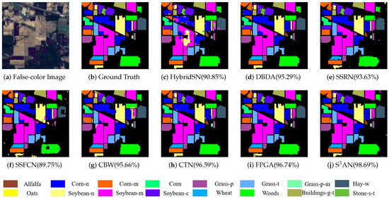
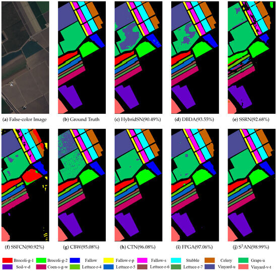
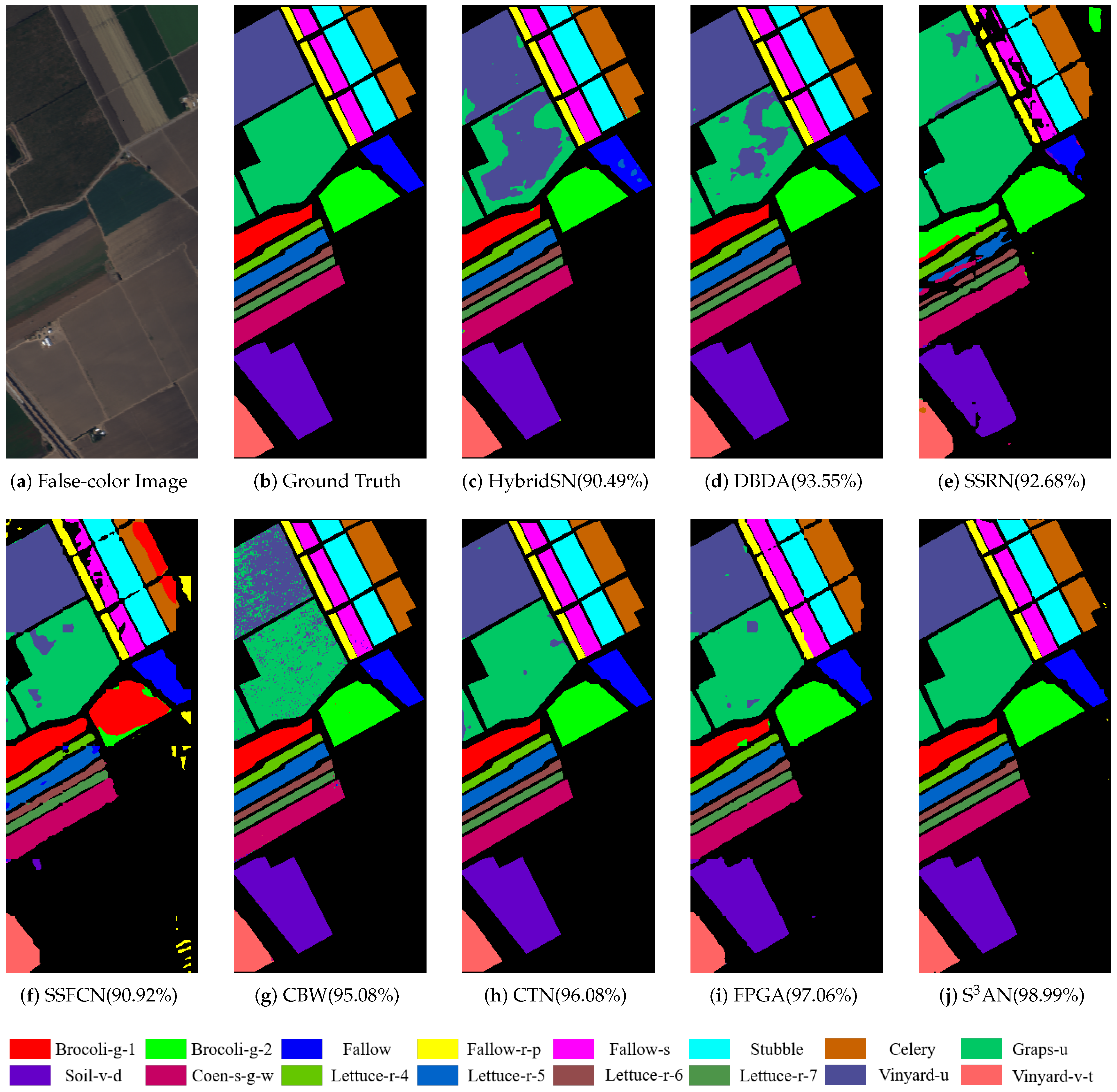
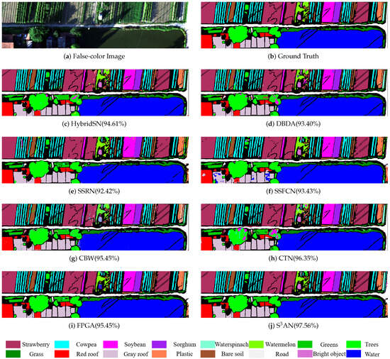
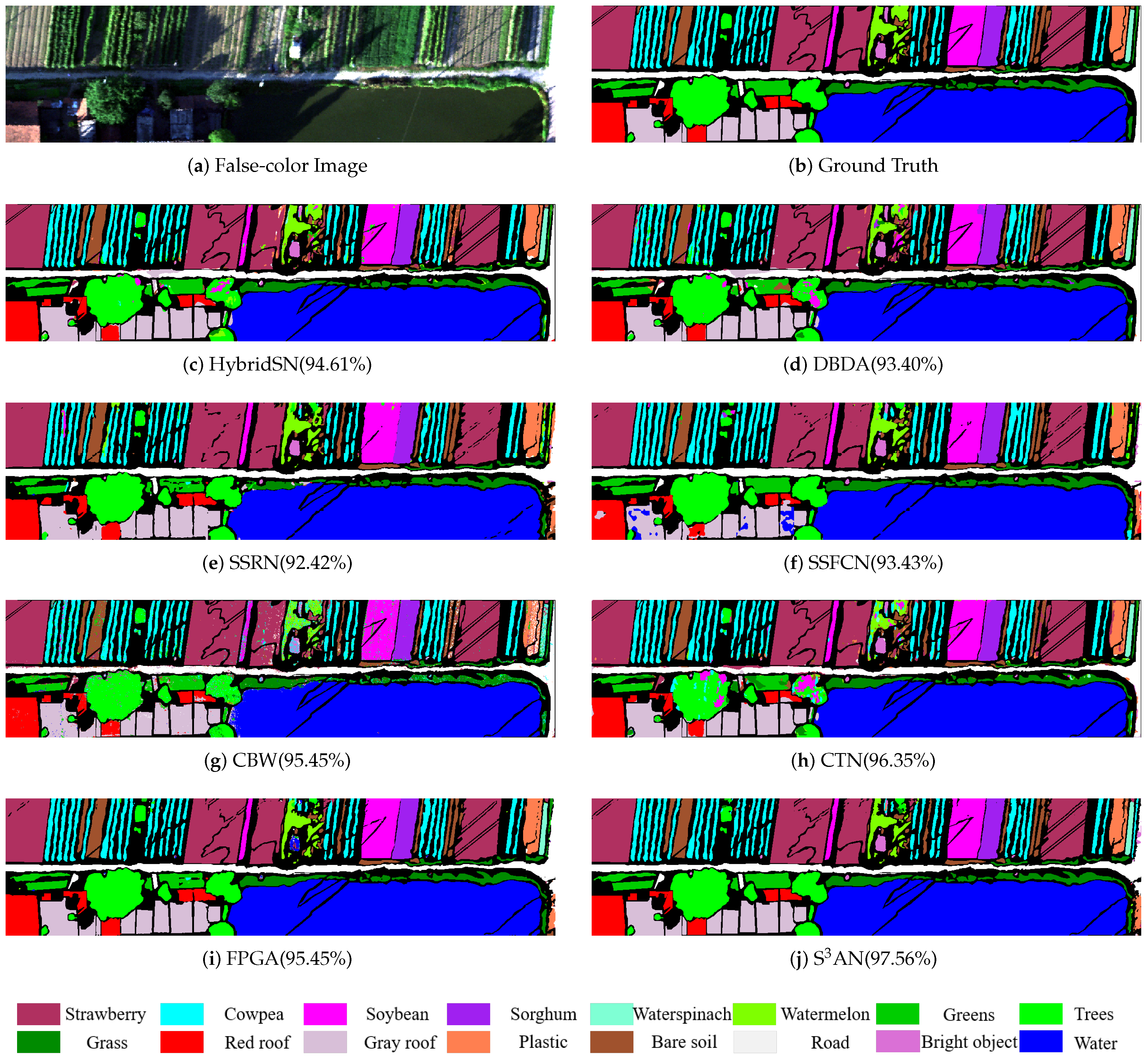
S³AN is compared with some state-of-the-art methods for HSI classification, which include HybridSN [13], DBDA [36], SSRN [15], SSFCN [16], CBW [43], CTN [46], and FPGA [17]. The classification results of different methods on three datasets are detailed in Table 2, Table 3 and Table 4, and the classification maps obtained by different methods are illustrated in Figure 6, Figure 7 and Figure 8.

Table 2. Classification results by different methods on the Indian Pines dataset.

Class	HybridSN	DBDA	SSRN	SSFCN	CBW	CTN	FPGA	S3AN
1	90.25 ± 0.86	95.15 ± 0.20	89.07 ± 0.95	56.24 ± 2.60	93.33 ± 1.64	95.23 ± 0.53	92.37 ± 0.15	99.16 ± 0.42
2	87.74 ± 0.29	93.76 ± 1.15	93.59 ± 0.63	89.65 ± 0.75	94.71 ± 0.85	94.28 ± 0.20	96.55 ± 0.12	91.55 ± 0.15
3	89.19 ± 0.92	89.61 ± 0.17	92.25 ± 0.99	95.45 ± 0.44	97.24 ± 0.23	94.61 ± 1.41	92.38 ± 0.37	96.33 ± 0.33
4	85.15 ± 1.94	92.89 ± 0.42	90.53 ± 1.36	92.62 ± 0.68	99.03 ± 0.07	98.14 ± 0.16	96.85 ± 0.25	98.18 ± 0.48
5	91.18 ± 0.08	94.66 ± 1.94	94.31 ± 2.56	95.44 ± 1.25	89.61 ± 1.21	98.62 ± 0.27	94.26 ± 0.31	97.75 ± 0.07
6	93.53 ± 0.25	96.45 ± 0.76	89.75 ± 0.72	74.96 ± 1.92	95.75 ± 2.91	97.60 ± 0.32	95.08 ± 1.25	99.60 ± 0.36
7	89.29 ± 0.88	95.33 ± 1.13	93.09 ± 1.02	85.66 ± 0.96	99.62 ± 0.15	96.15 ± 0.21	98.33 ± 0.88	95.89 ± 0.20
8	84.41 ± 0.64	97.01 ± 0.46	95.66 ± 1.79	93.50 ± 0.45	99.89 ± 0.04	99.30 ± 0.06	98.74 ± 0.65	97.03 ± 0.15
9	90.96 ± 1.12	95.62 ± 0.21	91.15 ± 0.56	91.75 ± 2.21	99.33 ± 0.21	89.99 ± 2.49	99.51 ± 0.42	96.96 ± 0.26
10	95.54 ± 1.28	92.74 ± 0.85	90.69 ± 0.21	84.85 ± 0.95	91.69 ± 1.35	99.18 ± 0.25	90.52 ± 1.13	99.51 ± 0.12
11	91.78 ± 2.21	94.11 ± 1.15	88.26 ± 2.24	89.15 ± 0.41	94.28 ± 0.84	96.83 ± 0.30	93.66 ± 0.16	95.45 ± 1.65
12	92.76 ± 0.86	96.35 ± 0.06	97.75 ± 1.09	93.96 ± 0.50	97.95 ± 0.39	98.50 ± 0.33	91.77 ± 3.71	96.33 ± 3.74
13	95.10 ± 0.42	94.18 ± 0.51	90.33 ± 0.57	89.31 ± 0.61	99.49 ± 0.28	99.45 ± 0.15	96.05 ± 0.85	98.45 ± 0.58
14	69.89 ± 2.98	89.72 ± 0.29	91.51 ± 0.66	91.99 ± 1.15	99.57 ± 0.04	99.21 ± 0.38	93.33 ± 2.59	99.76 ± 0.23
15	95.41 ± 0.68	88.96 ± 1.86	89.36 ± 0.30	92.25 ± 1.18	98.55 ± 0.16	98.86 ± 0.04	95.00 ± 0.23	98.50 ± 0.95
16	90.17 ± 0.11	95.99 ± 0.58	96.95 ± 0.29	90.96 ± 0.86	96.34 ± 0.31	94.99 ± 2.75	96.15 ± 0.58	96.88 ± 2.21
OA (%)	90.85 ± 0.15	95.29 ± 0.27	93.63 ± 0.05	89.75 ± 0.54	95.66 ± 0.24	96.59 ± 0.34	96.74 ± 0.17	98.69 ± 0.13
AA (%)	89.52 ± 0.42	93.91 ± 0.21	92.14 ± 0.73	87.98 ± 0.42	96.64 ± 0.50	96.93 ± 0.20	95.03 ± 0.20	97.33 ± 0.45
Kappa	0.9095 ± 0.004	0.9431 ± 0.002	0.9308 ± 0.003	0.8585 ± 0.002	0.9505 ± 0.002	0.9559 ± 0.004	0.9524 ± 0.004	0.9841 ± 0.002
Time (s)	8.78 ± 2.04	6.51 ± 1.03	7.62 ± 1.85	19.35 ± 2.55	3.58 ± 0.87	12.26 ± 1.46	5.4 ± 1.27	2.36 ± 0.99

Note that the values in bold are the highest.

Table 3. Classification results by different methods on the Salinas dataset.

Class	HybridSN	DBDA	SSRN	SSFCN	CBW	CTN	FPGA	S3AN
1	99.70 ± 0.04	94.89 ± 0.59	99.01 ± 0.16	63.82 ± 2.30	98.66 ± 0.05	99.50 ± 0.21	95.99 ± 0.54	99.32 ± 0.40
2	95.85 ± 0.12	98.22 ± 0.72	71.74 ± 3.56	99.55 ± 0.42	99.85 ± 0.11	94.96 ± 0.85	99.49 ± 0.36	98.75 ± 0.38
3	93.34 ± 0.37	92.85 ± 1.31	99.48 ± 0.12	96.74 ± 0.56	98.80 ± 0.25	99.39 ± 0.14	99.16 ± 0.60	99.93 ± 0.06
4	75.66 ± 2.64	95.89 ± 0.32	99.13 ± 0.14	87.99 ± 1.12	98.58 ± 0.60	97.71 ± 0.60	86.43 ± 1.59	99.51 ± 0.18
5	86.84 ± 1.95	87.26 ± 2.27	85.16 ± 1.57	86.56 ± 2.37	96.89 ± 0.32	97.47 ± 0.59	95.62 ± 0.55	96.65 ± 1.65
6	85.29 ± 0.62	83.79 ± 0.30	84.10 ± 2.92	90.55 ± 0.85	87.28 ± 1.74	99.27 ± 0.33	94.97 ± 0.20	95.74 ± 0.33
7	90.34 ± 0.58	85.75 ± 0.49	98.92 ± 0.53	90.24 ± 0.95	99.64 ± 0.03	87.38 ± 0.89	95.79 ± 0.56	98.41 ± 0.40
8	90.17 ± 0.62	86.11 ± 1.65	89.85 ± 0.36	93.61 ± 0.44	98.80 ± 0.16	99.61 ± 0.17	90.61 ± 1.65	95.22 ± 2.85
9	89.59 ± 0.66	91.18 ± 0.38	99.15 ± 0.39	95.35 ± 0.07	96.23 ± 0.85	98.77 ± 0.05	97.55 ± 0.97	98.79 ± 0.78
10	87.68 ± 3.31	89.99 ± 1.78	91.59 ± 0.51	85.49 ± 0.38	95.35 ± 0.64	90.61 ± 0.61	98.43 ± 0.43	95.46 ± 0.25
11	82.55 ± 0.47	92.35 ± 0.28	87.99 ± 0.83	89.71 ± 0.23	91.32 ± 0.79	96.89 ± 0.55	94.24 ± 0.45	98.22 ± 1.12
12	87.60 ± 2.80	98.96 ± 0.22	94.15 ± 0.95	79.75 ± 0.39	93.38 ± 0.85	94.37 ± 0.34	95.33 ± 1.92	97.75 ± 0.51
13	95.16 ± 1.15	95.19 ± 0.65	97.82 ± 0.55	95.07 ± 1.15	85.92 ± 2.38	99.43 ± 0.19	96.87 ± 0.45	96.36 ± 0.33
14	86.33 ± 0.22	90.55 ± 0.44	97.71 ± 0.60	99.51 ± 0.17	93.91 ± 0.33	98.06 ± 0.22	95.61 ± 0.16	99.73 ± 0.09
15	83.46 ± 0.58	91.76 ± 0.19	92.87 ± 0.71	90.96 ± 1.68	95.57 ± 0.45	85.39 ± 2.38	97.79 ± 0.66	97.55 ± 0.38
16	92.32 ± 0.14	94.33 ± 0.61	96.85 ± 0.28	89.65 ± 0.20	93.55 ± 0.20	97.77 ± 0.25	99.03 ± 0.22	99.85 ± 0.25
OA (%)	90.49 ± 0.55	93.55 ± 0.32	92.68 ± 0.39	90.92 ± 0.14	95.08 ± 0.25	96.08 ± 0.23	97.96 ± 0.65	98.59 ± 0.18
AA (%)	88.87 ± 0.86	91.82 ± 0.35	92.85 ± 0.25	89.66 ± 0.30	95.23 ± 0.34	96.03 ± 0.18	95.84 ± 0.35	97.95 ± 0.32
Kappa	0.9205 ± 0.004	0.933 ± 0.005	0.9033 ± 0.002	0.8993 ± 0.004	0.9413 ± 0.003	0.9468 ± 0.005	0.9774 ± 0.004	0.9792 ± 0.004
Time (s)	40.48 ± 5.45	40.33 ± 7.53	53.88 ± 5.95	102.99 ± 9.88	32.69 ± 4.50	42.68 ± 9.06	37.99 ± 3.37	25.09 ± 2.70

Note that the values in bold are the highest.

Table 4. Classification results by different methods on the HanChuan dataset.

Class	HybridSN	DBDA	SSRN	SSFCN	CBW	CTN	FPGA	S3AN
1	97.14 ± 0.74	95.41 ± 0.51	99.33 ± 0.32	99.50 ± 0.32	99.04 ± 0.37	99.32 ± 0.07	99.18 ± 0.27	99.41 ± 0.25
2	98.26 ± 0.36	99.71 ± 0.20	97.43 ± 0.62	98.17 ± 0.45	93.90 ± 0.88	97.43 ± 0.82	98.60 ± 0.55	96.04 ± 0.77
3	90.58 ± 1.18	84.97 ± 0.95	97.28 ± 0.95	99.75 ± 0.22	96.58 ± 1.78	97.27 ± 1.12	99.39 ± 0.64	99.69 ± 0.12
4	99.90 ± 0.06	86.97 ± 0.48	99.83 ± 0.31	98.39 ± 0.17	96.12 ± 1.10	99.83 ± 0.09	99.15 ± 0.41	99.75 ± 0.17
5	89.29 ± 0.95	98.02 ± 0.26	66.65 ± 3.75	12.03 ± 5.89	86.44 ± 2.40	86.65 ± 3.85	99.62 ± 0.23	99.96 ± 0.02
6	70.72 ± 2.25	81.72 ± 2.27	99.79 ± 0.15	78.83 ± 1.33	93.89 ± 0.56	97.99 ± 0.25	98.41 ± 0.51	98.40 ± 0.28
7	89.65 ± 0.60	99.82 ± 0.03	95.59 ± 0.29	99.06 ± 0.15	96.75 ± 0.49	95.59 ± 0.55	99.45 ± 0.13	99.92 ± 0.05
8	96.87 ± 0.49	93.40 ± 0.65	96.59 ± 0.66	97.16 ± 0.26	99.97 ± 0.02	96.59 ± 0.38	98.13 ± 0.19	97.99 ± 1.12
9	97.12 ± 0.85	94.37 ± 1.21	99.22 ± 0.54	99.68 ± 0.14	94.99 ± 0.38	99.22 ± 0.32	99.58 ± 0.26	98.70 ± 0.55
10	99.57 ± 0.31	98.68 ± 0.33	97.94 ± 0.36	96.51 ± 0.25	96.67 ± 0.65	97.94 ± 0.39	99.33 ± 0.75	99.59 ± 0.13
11	91.34 ± 0.25	89.54 ± 0.50	82.97 ± 0.89	95.26 ± 0.27	71.84 ± 2.78	82.97 ± 0.77	99.06 ± 0.50	99.78 ± 0.18
12	73.88 ± 4.62	86.46 ± 0.95	90.09 ± 1.44	85.57 ± 1.58	93.70 ± 0.49	90.09 ± 0.60	88.03 ± 2.42	83.7 ± 1.42
13	90.31 ± 0.37	88.17 ± 1.69	42.76 ± 5.12	97.92 ± 1.40	96.83 ± 0.71	96.49 ± 0.59	98.09 ± 1.37	97.71 ± 0.65
14	97.58 ± 0.15	98.35 ± 0.78	99.47 ± 0.31	99.77 ± 0.21	95.99 ± 0.67	99.46 ± 0.33	99.57 ± 0.25	99.65 ± 0.16
15	98.68 ± 0.63	99.13 ± 0.51	84.05 ± 0.55	65.87 ± 3.35	75.41 ± 3.81	84.04 ± 1.55	7.96 ± 3.89	68.11 ± 2.85
16	99.85 ± 0.05	99.73 ± 0.07	99.39 ± 0.16	97.56 ± 0.57	95.53 ± 0.55	99.93 ± 0.04	99.32 ± 0.25	99.58 ± 0.07
OA (%)	94.61 ± 0.31	93.4 ± 0.65	92.42 ± 0.75	93.43 ± 0.46	95.45 ± 0.46	96.35 ± 0.29	96.62 ± 0.56	97.56 ± 0.52
AA (%)	92.55 ± 0.28	92.32 ± 0.44	90.52 ± 0.66	88.81 ± 0.60	92.78 ± 0.35	95.05 ± 0.46	92.68 ± 0.60	96.23 ± 0.31
Kappa	0.9447 ± 0.004	0.9204 ± 0.004	0.9191 ± 0.006	0.9288 ± 0.007	0.9429 ± 0.006	0.9668 ± 0.004	0.9505 ± 0.006	0.9769 ± 0.004
Time (s)	209.37 ± 9.96	404.83 ± 20.38	371.49 ± 10.44	508.42 ± 20.51	246.42 ± 16.40	313.26 ± 17.65	169.79 ± 3.15	121.09 ± 6.98

Note that the values in bold are the highest.

Figure 6. Classification maps of the different methods on the Indian Pines dataset.

Figure 7. Classification maps of the different methods on the Salinas dataset.

Figure 8. Classification maps of the different methods on the HanChuan dataset.

4.3.1. Classification Results on Indian Pines Dataset

Table 2 shows that CNN-based methods obtain reasonable classification results, where the $OA$ of S³AN and FPGA reaches 98.69% and 96.74%, respectively. It is shown that CNN-based methods have advantages in capturing the correlation of spectral–spatial features. As for the attention mechanism-based methods, CBW and CTN, with 95.66% and 96.59% of $OA$. In addition, SSFCN is able to directly deal with the entire HSI, and it achieves 89.75% and 87.98% of $OA$ and $AA$, respectively. However, for objects with small samples, such as categories 1 and 6, the classification accuracies of SSFCN are only 56.24% and 74.96%. It is illustrated that the Indian Pines dataset has imbalanced training samples, and objects with a larger number of samples are beneficial for feature learning. In addition, S³AN introduces the RRM module to transform HSI into dimension-reduced features. Hence, the inference time of the entire image is reduced to 2.36 s, which is much lower than that of SSFCN and CTN.

As shown in Figure 6, there are fewer misclassifications in the classification map of S³AN compared with other methods. For example, in the Soybean-m and Corn-n regions, S³AN shows a good visualization and obtains better classification results than its competitors. Meanwhile, attention mechanism-based methods, such as CTN and CBW, have better visualization performance than SSFCN. However, some misclassification still occurs in DBDA and SSRN because the approximate features are difficult to distinguish. In contrast, S³AN introduces controllable factors to balance the differences in spectral–spatial features and enhance the sensitivity of attention mechanisms. Therefore, it is suitable for recognizing objects with small samples, such as the Corn and Soybean categories.

4.3.2. Classification Results on Salinas Dataset

Table 3 shows that the attention mechanism-based methods achieve better classification results than the CNN-based methods. Among them, the $OA$ of S³AN obtains about a 10% improvement, compared to HybridSN and SSFCN. It shows that attention mechanism-based methods are able to focus on the important objects to improve the classification accuracy. Moreover, S³AN introduces the sensorial attention mechanism to search for the labeled pixels, and guides the model to focus on the objects of each category simultaneously. Therefore, compared to FPGA, S³AN is more stable in the classification of each category and has a 2.11% improvement in $AA$. Further, the inference time of S³AN for the entire image is 25.09 s, which is about 20 s faster than DBDA and SSRN.

As shown in Figure 7, the classification map of S³AN shows the distribution of different objects is more clear than other methods. This indicates that the attention mechanism with controllable factors plays an active role in feature learning. Although DBDA and SSRN utilize attention mechanisms for HSI classification, their classification maps still contain some regions that are not accurately recognized. For approximate features that are difficult to distinguish, such as Vineyard and Grape categories, these attention mechanism-based methods still suffer from some misclassification. It is thought that unsuitable evaluation manners in attention mechanisms lead to inaccurate attention regions, which influence classification results. In contrast, CTN and S³AN are able to accurately locate important objects and obtain classification maps that are close to ground truth.

4.3.3. Classification Results on HanChuan Dataset

Table 4 shows that the methods with label processing, such as FPGA and S³AN, obtain better classification results than other methods. Among them, GS2 is introduced into FPGA for label-stratified sampling, with the $OA$ and $Kappa$ coefficients reaching 96.62% and 0.9505, respectively. S³AN processes the pseudo label by sensorial attention mechanism, which further improves the $OA$ to 97.56%. It is indicated that the location and category information of different objects in the pseudo label plays a positive role in HSI classification and contributes to the results of the S³AN. Since the HanChuan dataset contains a large number of labeled samples, obtaining classification results requires a long inference time. S³AN performs redundancy reduction before feature learning, and completes inference in only 121.09 s, with a much lower time cost than SSRN, SSFCN, and DBDA. In addition, S³AN introduces Trans-Conv to mitigate the dimensional mutation, which provides a ramp for channel transition, and it retains some details for label prediction, therefore, a better consistency is obtained with a $Kappa$ coefficient of 0.9769 compared to other methods.

As shown in Figure 8, HybridSN and CTN show few misclassifications in the Tree and Roof categories. Since these two categories of objects are in shadow and glare, it is difficult to recognize them directly even by human eyes, which brings challenges to classification. Compared to CTN, S³AN is more concerned with the processing of details and accurately distinguishing Grass and Watermelon categories. Moreover, in the shadow areas, the classification result of S³AN is better than other methods and has sharper category boundaries of details. This indicates that S³AN is efficient in enhancing the representation of details and is robust enough to recognize objects in shadow areas.

4.3.4. Confusion Matrix

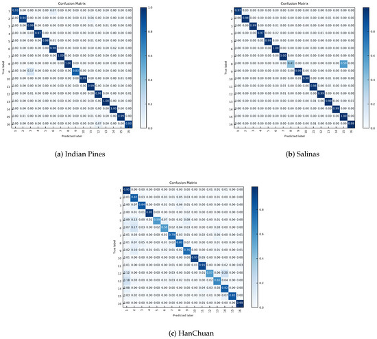
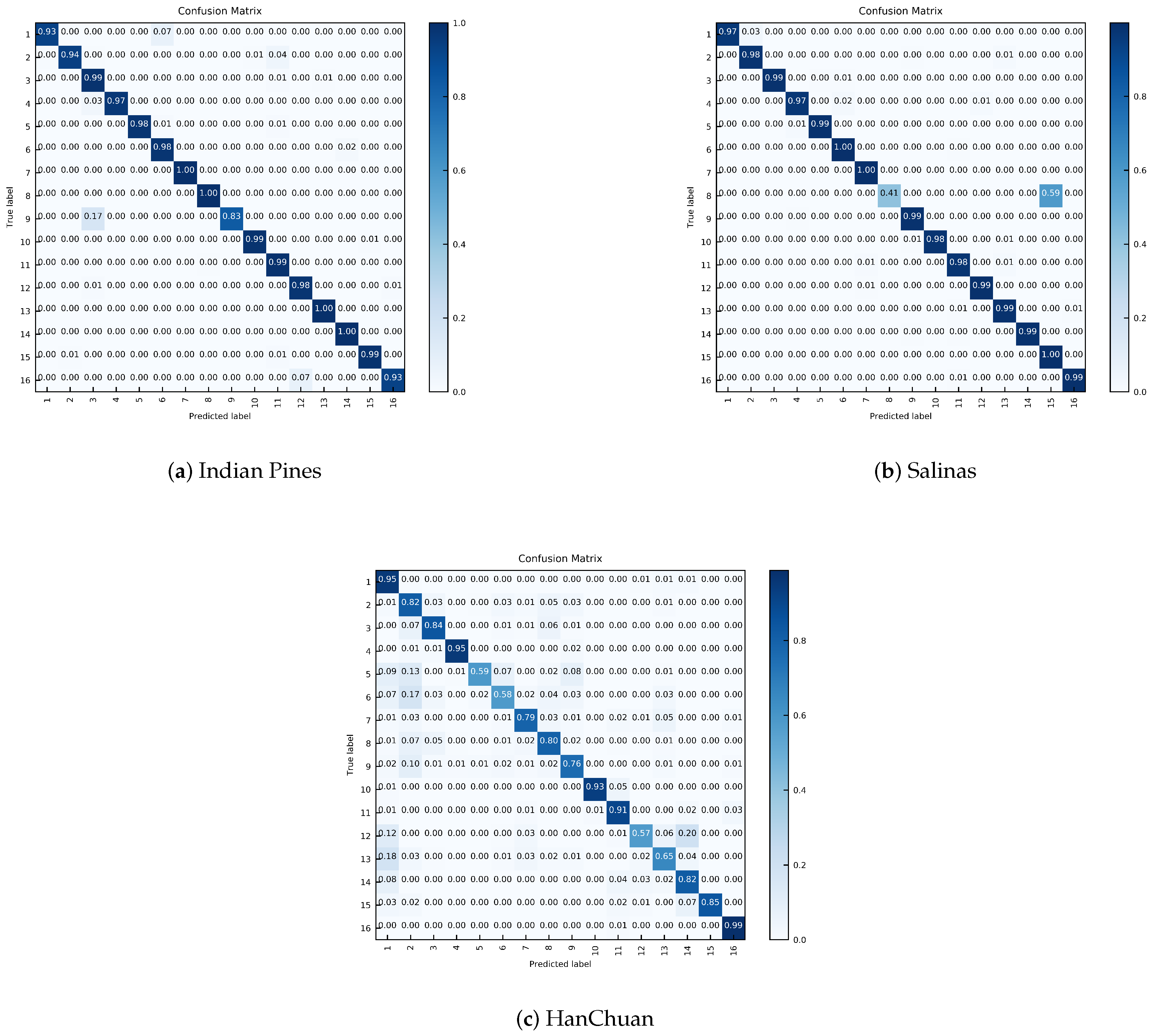
As shown in Figure 9, to show the classification ability of S³AN, the results of confusion matrices on three datasets are visualized. From Figure 9b, it is seen that on the Indian Pines dataset, a high classification accuracy is obtained for all categories except for the Corn category. Notice that the S³AN also accurately recognizes the Grass-p category that contains a small number of samples. For the Salinas dataset, the proposed method showed misclassification for Grap objects due to the extreme similarity of the Grap and Vinyard categories, but it is still able to accurately recognize ground objects in other categories. From Figure 9c, it is observed that the HanChuan dataset has an imbalance of samples, where most of the samples are distributed in the categories of Strawberry and Water, which increases the difficulty of HSI classification, and the S³AN still obtains a satisfactory classification results. Moreover, the proposed method is able to accurately recognize objects with a small percentage of samples, such as the categories Sorghum, Watermelon, and Bright, which suggests that the methods for retaining details in the S³AN play a positive effect.

Figure 9. The confusion matrices visualization of S³AN on the three datasets.

5. Discussion

5.1. Discussion of Controllable Factors

To analyze the influence of controllable factors, S³AN with no controllable factors is set as the baseline and gradually adds DE-Pooling and Adapt-Conv to observe the change in classification result.

As shown in Table 5, the $OA$ of the baseline is lower on three datasets, it is suggested that the spectral-spatial-sensorial attention mechanism without controllable factors makes it difficult to distinguish the continuous and approximate features, and results in the inaccurate delineation of attention regions. Then, DE-Pooling is added into attention mechanisms, and the $OA$ is increased from 65.03% to 96.18% on the Salinas dataset. It is shown that DE-Pooling significantly improves the sensitivity of attention mechanisms and controls the updating of attention weights to balance the differences in spectral–spatial features. Then, DE-Pooling and Adapt-Conv are added into attention mechanisms simultaneously, and further improve the classification result. In particular, the $OA$ reaches 98.41% on the Indian Pines dataset, which indicates that boosting the weight interaction contributes to enhancing the sensitivity of the attention mechanism and improves the classification result.

Table 5. Classification results by different controllable factors.

Dataset	Method	DE-Pooling	Adapt-Conv	OA (%)	AA (%)	Kappa
Indian Pines	Baseline	-	-	83.19 ± 1.14	81.32 ± 1.68	0.7816 ± 0.075
	DE-Pooling	✓	-	96.57 ± 0.65	96.85 ± 1.60	0.9379 ± 0.097
	DE-Pooling + Adapt-Conv	✓	✓	98.41 ± 0.44	97.55 ± 0.60	0.9591 ± 0.059
Salinas	Baseline	-	-	65.03 ± 3.35	63.77 ± 2.70	0.5952 ± 0.031
	DE-Pooling	✓	-	95.18 ± 0.65	94.35 ± 0.89	0.9331 ± 0.016
	DE-Pooling + Adapt-Conv	✓	✓	98.09 ± 0.38	97.42 ± 0.55	0.9799 ± 0.012
HanChuan	Baseline	-	-	71.83 ± 4.78	69.52 ± 3.96	0.6607 ± 0.036
	DE-Pooling	✓	-	95.61 ± 0.55	95.22 ± 0.27	0.9494 ± 0.031
	DE-Pooling + Adapt-Conv	✓	✓	97.51 ± 0.11	96.89 ± 0.28	0.9673 ± 0.003

5.2. Discussion of Sensorial Attention Mechanism

The sensorial attention mechanism mainly contributes to positioning the labeled pixels and emphasizing the details in the semantic feature map [47]. To verify its effectiveness, experiments are conducted based on S³AN with the presence or absence of the sensorial attention mechanism as the variable.

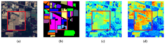
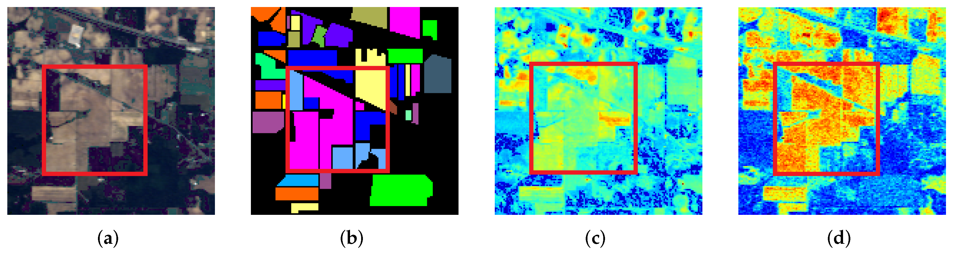
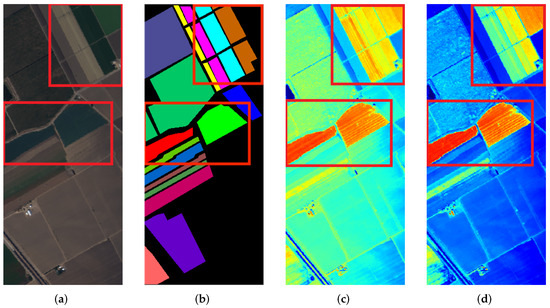
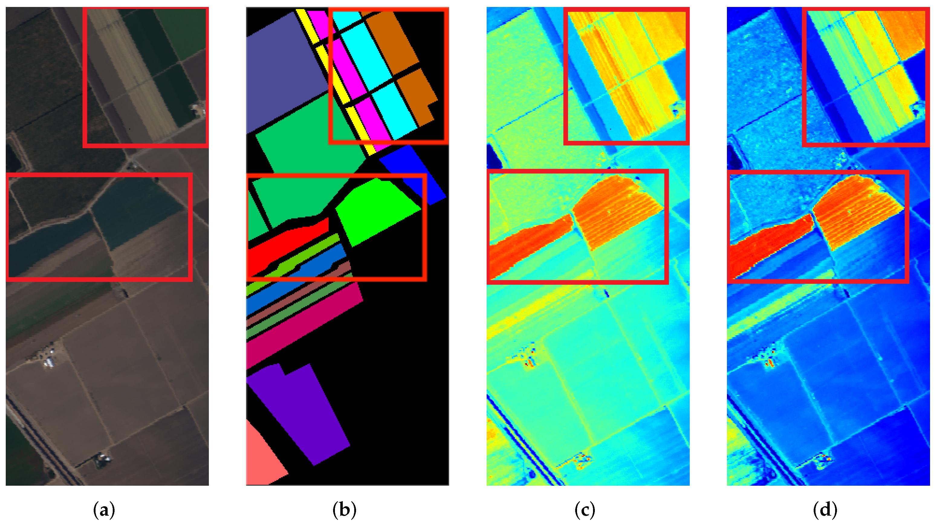
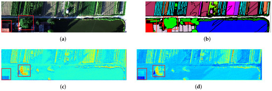
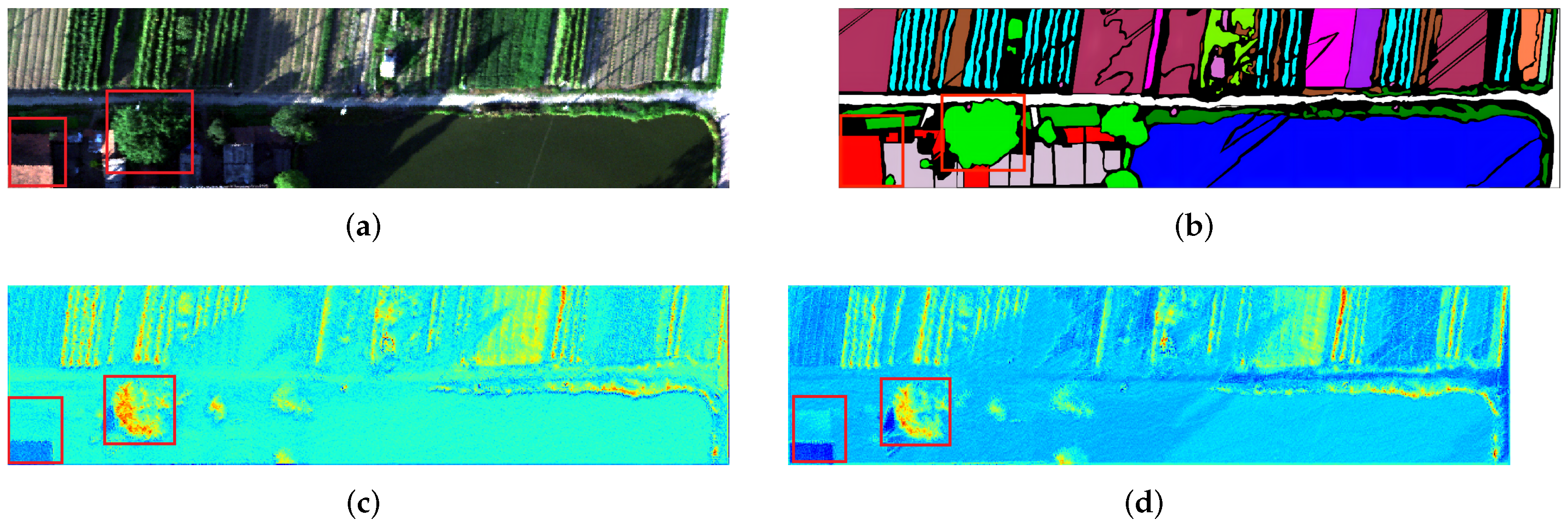
As shown in Figure 10, Figure 11 and Figure 12, for the semantic feature map without the sensorial attention mechanism, little pixels are highlighted to turn into the attention regions, and the difference in adjacent features is insufficient. In contrast, the semantic feature map with sensorial attention mechanism guidance expresses the important object areas and emphasizes details within a few pixels. Note the areas of the red box, the sensorial attention mechanism significantly highlights the labeled pixels and distinguishes the approximate features with different degrees of attention regions. Specifically, for the HanChuan dataset, the sensorial attention mechanism also focuses on the Roof and Tree areas in the shadow. Although the shadow areas affect the representation of spatial features and increase the difficulty of distinguishing the approximate features, the sensorial attention mechanism still accurately positions the objects based on the category information of the pseudo label. In addition, with the emphasis on the sensorial attention mechanism, the delineation of attention regions in the semantic feature map is close to the real situation. Therefore, the experimental results demonstrate that the sensorial attention mechanism is efficient to emphasize the details of semantic feature maps, and adapts to HSI classification.

Figure 10. Visualization of attention regions for semantic feature map on Indian Pines dataset: (a) false-color image, (b) ground truth, (c) visualization of feature map without sensorial attention mechanism, (d) visualization of feature map with sensorial attention mechanism. Blue indicates lower attention values and red indicates higher attention values.

Figure 11. Visualization of attention regions for semantic feature map on Salinas dataset: (a) false-color image, (b) ground truth, (c) visualization of feature map without sensorial attention mechanism, (d) visualization of feature map with sensorial attention mechanism.

Figure 12. Visualization of attention regions for semantic feature map on HanChuan dataset: (a) false-color image, (b) ground truth, (c) visualization of feature map without sensorial attention mechanism, (d) visualization of feature map with sensorial attention mechanism.

5.3. Discussion of Trans-Conv Layers

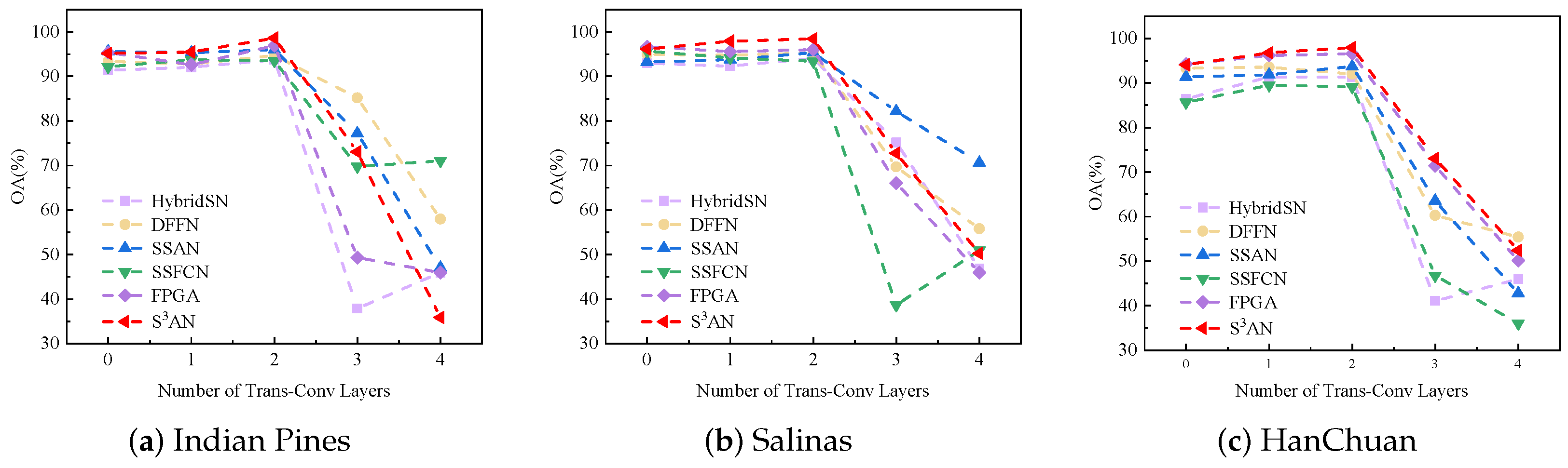
Trans-Conv mitigates the dimensional mutation by adding convolutional layers in the prediction layer to achieve the transition of details. To analyze the effect of depth for Trans-Conv on the classification result, different numbers of Trans-Conv layers are added to the state-of-the-art methods, and the $OA$ variations are observed to determine the appropriate depth of Trans-Conv.

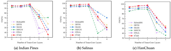
As shown in Figure 13, for the Indian Pines dataset, there is an additional improvement of about 1% in $OA$ for HybridSN, SSFCN, and S³AN when using only one Trans-Conv layer. The $OA$ of S³AN reaches about 97% with the addition of two Trans-Conv layers, which is due to convolutional layers further extracting details while transforming the feature dimensions. However, when the number of Trans-Conv layers is set to three, the decrease in $OA$ is rapid. Inappropriate Trans-Conv layers change the abstract semantic information and result in a decrease in the representation of details. Moreover, for the Salinas and HanChuan datasets with two Trans-Conv layers set up, the $OA$ of the different methods reaches about 96%. The appropriate Trans-Conv layers gradually decreasing the dimension are able to retain details, and contribute to improving the classification accuracy. Therefore, the dimensional reduction coefficient r is set to two, which means the dimension of the feature map decays by half.

Figure 13. The $OA$ of state-of-the-art methods with different Trans-Conv layers on three datasets.

5.4. Discussion of Selected Bands

RRM selects the important bands to construct dimension-reduced features based on spectral attention weights, to analyze the effect of the number of selected bands on classification results, experiments are conducted based on different numbers of selected bands and observe the variation in the classification accuracy.

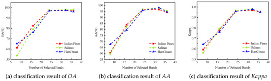
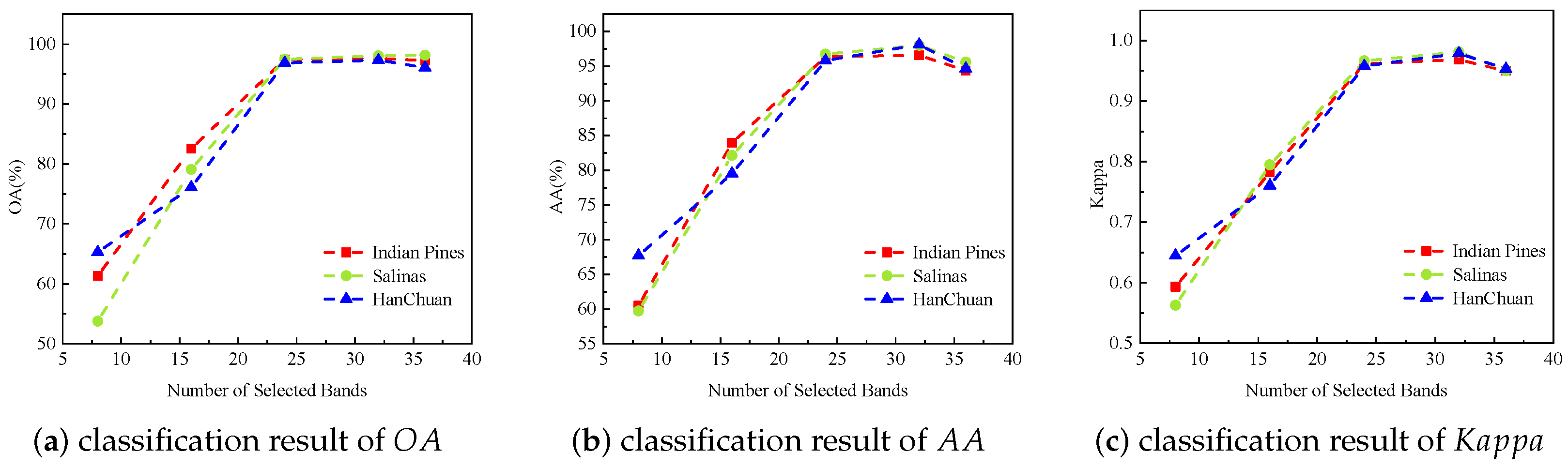
As shown in Table 6, when the number of selected bands is 8, the $OA$ of S³AN on 3 datasets is limited to about 60% because important bands are not fully selected for feature learning. Then, the $AA$ is significantly increased from 60% to about 80% when the number of selected bands is set to 16. Further, the $OA$ reaches about 97% and the classification result gradually stabilizes when the number of selected bands is increased to 36. Figure 14 illustrates the trend of classification results for the different numbers of selected bands. The variation in classification results shows that the insufficient number of selected bands makes it difficult to obtain a satisfactory $OA$, and the inference time is increased by too many bands. Therefore, an appropriate number of selected bands is beneficial for model convergence and improving the speed of inference. Further, some continuous bands are selected by RRM, since the physical characteristics of the object are saved in these bands and have better feature representation. S³AN applies redundancy reduction as a pre-processing to improve the speed of inference without sacrificing $OA$ as much as possible, so that the inference time on 3 datasets is reduced to 2.95 s, 25.59 s, and 120.55 s, respectively.

Table 6. Classification results of different numbers of selected bands on three datasets.

Dataset	Number	Selected Band	OA (%)	AA (%)	Kappa	Time (s)
Indian Pines	8	[102,104,…,198]	61.33 ± 5.56	60.51 ± 4.70	0.5933 ± 0.093	1.66 ± 0.30
	16	[56,102,…,199]	82.60 ± 2.33	83.95 ± 1.16	0.7827 ± 0.062	1.85 ± 0.31
	24	[18,56,…,199]	97.45 ± 0.18	96.37 ± 0.25	0.9615 ± 0.005	2.07 ± 0.29
	32	[12,18,…,199]	97.63 ± 0.21	96.59 ± 0.09	0.9689 ± 0.003	2.41 ± 0.29
	36	[12,17,…,199]	97.25 ± 0.30	94.35 ± 0.27	0.9500 ± 0.003	2.95 ± 0.30
Salinas	8	[37,38,…,197]	53.77 ± 5.53	59.73 ± 3.95	0.5630 ± 0.052	12.32 ± 1.56
	16	[12,19,…,200]	79.09 ± 2.61	82.14 ± 3.35	0.7949 ± 0.079	15.61 ± 2.05
	24	[8,9,12,…,200]	97.51 ± 0.22	96.75 ± 0.37	0.9665 ± 0.012	18.44 ± 3.32
	32	[4,5,6,…,200]	98.05 ± 0.16	98.00 ± 0.11	0.9811 ± 0.007	25.89 ± 2.98
	36	[4,5,6,…,200]	98.16 ± 0.29	95.58 ± 0.36	0.9503 ± 0.015	29.59 ± 3.75
HanChuan	8	[0,3,10,...,254]	65.30 ± 2.49	67.72 ± 3.60	0.6447 ± 0.071	64.35 ± 8.83
	16	[0,3,10,…,272]	76.11 ± 3.55	79.55 ± 3.70	0.7605 ± 0.063	89.05 ± 7.99
	24	[1,3,10,…,272]	96.89 ± 0.19	95.80 ± 0.23	0.9578 ± 0.015	96.16 ± 10.80
	32	[1,3,10,…,273]	97.32 ± 0.25	98.11 ± 0.19	0.9790 ± 0.010	120.55 ± 9.55
	36	[1,2,3,…,273]	96.09 ± 0.51	94.65 ± 1.01	0.9532 ± 0.026	164.89 ± 10.66

Figure 14. The classification results of different numbers of selected bands on three datasets.

6. Conclusions

In this paper, an effective S³AN is proposed for HSI classification. Driven by controllable factors (DE-Pooling and Adapt-Conv), attention mechanisms are able to distinguish differences in approximate spectral–spatial features and to generate more reliable regions of interest. To reduce the computational cost, the controllable spectral attention mechanism accurately highlights representative bands in the HSI and reduces spectral redundancy. The controllable spatial attention mechanism cooperates with cross-layer feature learning to automatically extract local contextual semantics, and enhances the ability of deep and shallow feature interaction. In addition, the controllable sensorial attention mechanism explores the location and category information of ground objects, which further enhances the HSI classification results. The experimental results on three public HSI datasets show that the proposed method enables fast and accurate HSI classification.

Based on the experimental results, it is known that the proposed controllable attention mechanisms are adaptable to the complex feature environment of HSI. However, all results are obtained under the condition of labeled datasets, which require a lot of time for labeling. In contrast, producing unlabeled datasets reduces the workload, and it is interesting to explore the self-supervised HSI classification in the future.

References

- He, L.; Li, J.; Liu, C.; Li, S. Recent advances on spectral–spatial hyperspectral image classification: An overview and new guidelines. IEEE Trans. Geosci. Remote Sens. 2018, 56, 1579–1597. [Google Scholar] [CrossRef] [Scilit]
- Paoletti, M.; Haut, J.; Plaza, J.; Plaza, A. Deep learning classifiers for hyperspectral imaging: A review. ISPRS J. Photogramm. Remote Sens. 2019, 158, 279–317. [Google Scholar] [CrossRef] [Scilit]
- Dong, Y.; Liang, T.; Zhang, Y.; Du, B. Spectral–spatial weighted kernel manifold embedded distribution alignment for remote sensing image classification. IEEE Trans. Cybern. 2021, 51, 3185–3197. [Google Scholar] [CrossRef] [Scilit] [PubMed]
- Zhou, Y.; Peng, J.; Chen, C. Dimension reduction using spatial and spectral regularized local discriminant embedding for hyperspectral image classification. IEEE Trans. Geosci. Remote Sens. 2014, 53, 1082–1095. [Google Scholar] [CrossRef] [Scilit]
- Zhou, Y.; Wei, Y. Learning hierarchical spectral–spatial features for hyperspectral image classification. IEEE Trans. Cybern. 2016, 46, 1667–1678. [Google Scholar] [CrossRef] [Scilit] [PubMed]
- Zhang, F.; Du, B.; Zhang, L.; Zhang, L. Hierarchical feature learning with dropout k-means for hyperspectral image classification. Neurocomputing 2016, 187, 75–82. [Google Scholar] [CrossRef] [Scilit]
- Wang, M.; Wu, C.; Wang, L.; Xiang, D.; Huang, X. A feature selection approach for hyperspectral image based on modified ant lion optimizer. Knowl. Based Syst. 2019, 168, 39–48. [Google Scholar] [CrossRef] [Scilit]
- Xia, J.; Ghamisi, P.; Yokoya, N.; Iwasaki, A. Random forest ensembles and extended multiextinction profiles for hyperspectral image classification. IEEE Trans. Geosci. Remote Sens. 2018, 56, 202–216. [Google Scholar] [CrossRef] [Scilit]
- Wang, M.; Yan, Z.; Luo, J.; Ye, Z.; He, P. A band selection approach based on wavelet support vector machine ensemble model and membrane whale optimization algorithm for hyperspectral image. Appl. Intell. 2021, 51, 7766–7780. [Google Scholar] [CrossRef] [Scilit]
- Fang, L.; Li, S.; Kang, X.; Benediktsson, J. Spectral–spatial hyperspectral image classification via multiscale adaptive sparse representation. IEEE Trans. Geosci. Remote Sens. 2014, 52, 7738–7749. [Google Scholar] [CrossRef] [Scilit]
- Zhou, H.; Zhang, X.; Zhang, C.; Ma, Q. Quaternion convolutional neural networks for hyperspectral image classification. Eng. Appl. Artif. Intell. 2023, 123, 106234. [Google Scholar] [CrossRef] [Scilit]
- Zhao, Z.; Hu, D.; Wang, H.; Yu, X. Convolutional transformer network for hyperspectral image classification. IEEE Trans. Geosci. Remote Sens. 2022, 19, 6009005. [Google Scholar] [CrossRef] [Scilit]
- Roy, S.; Krishna, G.; Dubey, S.; Chaudhuri, B. HybridSN: Exploring 3-D–2-D CNN feature hierarchy for hyperspectral image classification. IEEE Geosci. Remote Sens. Lett. 2019, 17, 277–281. [Google Scholar] [CrossRef] [Scilit]
- Dalal, A.; Cai, Z.; Al-Qaness, M.; Dahou, A.; Alawamy, E.; Issaka, S. Compression and reinforce variation with convolutional neural networks for hyperspectral image classification. Appl. Soft Comput. 2022, 130, 109650. [Google Scholar]
- Zhong, Z.; Li, J.; Luo, Z.; Chapman, M. Spectral–spatial residual network for hyperspectral image classification: A 3-D Deep Learning Framework. IEEE Trans. Geosci. Remote Sens. 2018, 56, 847–858. [Google Scholar] [CrossRef] [Scilit]
- Xu, Y.; Du, B.; Zhang, L. Beyond the patchwise classification: Spectral-spatial fully convolutional networks for hyperspectral image classification. IEEE Trans. Big Data 2020, 6, 492–506. [Google Scholar] [CrossRef] [Scilit]
- Zheng, Z.; Zhong, Y.; Ma, A.; Zhang, L. FPGA: Fast patch-free global learning framework for fully end-to-end hyperspectral image classification. IEEE Trans. Geosci. Remote Sens. 2020, 58, 5612–5626. [Google Scholar] [CrossRef] [Scilit]
- Yang, X.; Cao, W.; Lu, Y.; Zhou, Y. Hyperspectral image transformer classification networks. IEEE Trans. Geosci. Remote Sens. 2022, 60, 5528715. [Google Scholar] [CrossRef] [Scilit]
- Huang, Z.; Wang, X.; Wei, Y.; Huang, L.; Shi, H.; Liu, W.; Huang, T. Criss-cross attention for semantic segmentation. IEEE Trans. Pattern Anal. Mach. Intell. 2023, 45, 6896–6908. [Google Scholar] [CrossRef] [Scilit] [PubMed]
- Wang, X.; Zhu, J.; Feng, Y.; Wang, L. MS2CANet: Multiscale spatial–spectral cross-modal attention network for hyperspectral image and LiDAR classification. IEEE Geosci. Remote Sens. Lett. 2024, 21, 5501505. [Google Scholar] [CrossRef] [Scilit]
- Hu, J.; Shen, L.; Albanie, S.; Sun, G.; Wu, E. Squeeze-and-excitation networks. IEEE Trans. Pattern Anal. Mach. Intell. 2020, 42, 2011–2023. [Google Scholar] [CrossRef] [Scilit] [PubMed]
- Woo, S.; Park, J.; Lee, J.Y.; Kweon, I.S. Cbam: Convolutional block attention module. In Proceedings of the European Conference on Computer Vision (ECCV), Munich, Germany, 8–14 September 2018; pp. 3–19. [Google Scholar]
- Wang, Q.; Wu, B.; Zhu, P.; Li, P.; Zuo, W.; Hu, Q. ECA-Net: Efficient channel attention for deep convolutional neural networks. In Proceedings of the IEEE/CVF Conference on Computer Vision and Pattern Recognition, Seattle, WA, USA, 13–19 June 2020; pp. 1153–11542. [Google Scholar]
- Shi, C.; Wu, H.; Wang, L. A feature complementary attention network based on adaptive knowledge filtering for hyperspectral image classification. IEEE Trans. Geosci. Remote Sens. 2023, 61, 5527219. [Google Scholar] [CrossRef] [Scilit]
- Xing, C.; Duan, C.; Wang, Z.; Wang, M. Binary feature learning with local spectral context-aware attention for classification of hyperspectral images. Pattern Recognit. 2023, 134, 109123. [Google Scholar] [CrossRef] [Scilit]
- Zhao, Z.; Wang, H.; Yu, X. Spectral-spatial graph attention network for semisupervised hyperspectral image classification. IEEE Geosci. Remote Sens. Lett. 2021, 19, 5503905. [Google Scholar] [CrossRef] [Scilit]
- Hou, Q.; Zhou, D.; Feng, J. Coordinate attention for efficient mobile network design. In Proceedings of the IEEE/CVF Conference on Computer Vision and Pattern Recognition, Nashville, TN, USA, 20–25 June 2021; pp. 13713–13722. [Google Scholar]
- Wang, F.; Jiang, M.; Qian, C.; Yang, S.; Li, C.; Zhang, H.; Wang, X.; Tang, X. Residual attention network for image classification. In Proceedings of the IEEE Conference on Computer Vision and Pattern Recognition, Honolulu, HI, USA, 21–26 July 2017; pp. 3156–3164. [Google Scholar]
- Wang, W.; Liu, F.; Liu, J.; Xiao, L. Cross-domain few-shot hyperspectral image classification with class-wise attention. IEEE Trans. Geosci. Remote Sens. 2023, 61, 5502418. [Google Scholar] [CrossRef] [Scilit]
- Roy, S.; Deria, A.; Shah, C.; Haut, J.; Du, Q.; Plaza, A. Spectral–spatial morphological attention transformer for hyperspectral image classification. IEEE Trans. Geosci. Remote Sens. 2023, 61, 5503615. [Google Scholar] [CrossRef] [Scilit]
- Zhao, F.; Li, S.; Zhang, J.; Liu, H. Convolution transformer fusion splicing network for hyperspectral image classification. IEEE Geosci. Remote Sens. Lett. 2023, 20, 5501005. [Google Scholar] [CrossRef] [Scilit]
- Mou, L.; Ghamisi, P.; Zhu, X. Unsupervised spectral–spatial feature learning via deep residual Conv–Deconv network for hyperspectral image classification. IEEE Trans. Geosci. Remote Sens. 2017, 56, 391–406. [Google Scholar] [CrossRef] [Scilit]
- Lin, S.; Zhang, M.; Cheng, X.; Shi, L.; Gamba, P.; Wang, H. Dynamic low-rank and sparse priors constrained deep autoencoders for hyperspectral anomaly detection. IEEE Trans. Instrum. Meas. 2024, 73, 2500518. [Google Scholar] [CrossRef] [Scilit]
- Pan, B.; Xu, X.; Shi, Z.; Zhang, N.; Luo, H.; Lan, X. DSSNet: A simple dilated semantic segmentation network for hyperspectral imagery classification. IEEE Geosci. Remote Sens. Lett. 2020, 17, 1968–1972. [Google Scholar] [CrossRef] [Scilit]
- Pu, C.; Huang, H.; Yang, L. An attention-driven convolutional neural network-based multi-level spectral–spatial feature learning for hyperspectral image classification. Expert Syst. Appl. 2021, 185, 115663. [Google Scholar] [CrossRef] [Scilit]
- Li, R.; Zheng, S.; Duan, C.; Yang, Y.; Wang, X. Classification of hyperspectral image based on double-branch dual-attention mechanism network. Remote Sens. 2020, 12, 582. [Google Scholar] [CrossRef] [Scilit]
- Zhu, M.; Jiao, L.; Liu, F.; Yang, S.; Wang, J. Residual spectral–spatial attention network for hyperspectral image classification. IEEE Trans. Geosci. Remote Sens. 2020, 59, 449–462. [Google Scholar] [CrossRef] [Scilit]
- Sun, H.; Zheng, X.; Lu, X.; Wu, S. Spectral–spatial attention network for hyperspectral image classification. IEEE Trans. Geosci. Remote Sens. 2019, 58, 3232–3245. [Google Scholar] [CrossRef] [Scilit]
- Cheng, X.; Zhang, M.; Lin, S.; Li, Y.; Wang, H. Deep self-representation learning framework for hyperspectral anomaly detection. IEEE Trans. Instrum. Meas. 2023, 73, 5002016. [Google Scholar] [CrossRef] [Scilit]
- Cai, Y.; Liu, X.; Cai, Z. BS-Nets: An end-to-end framework for band selection of hyperspectral image. IEEE Trans. Geosci. Remote Sens. 2019, 58, 1969–1984. [Google Scholar] [CrossRef] [Scilit]
- Nandi, U.; Roy, S.; Hong, D.; Wu, X.; Chanussot, J. TAttMSRecNet: Triplet-attention and multiscale reconstruction network for band selection in hyperspectral images. Expert Syst. Appl. 2023, 212, 118797. [Google Scholar] [CrossRef] [Scilit]
- Chen, Y.; Jiang, H.; Li, C.; Jia, X.; Ghamisi, P. Deep feature extraction and classification of hyperspectral images based on convolutional neural networks. IEEE Trans. Geosci. Remote Sens. 2016, 54, 6232–6251. [Google Scholar] [CrossRef] [Scilit]
- Zhao, L.; Yi, J.; Li, X.; Hu, W.; Wu, J.; Zhang, G. Compact band weighting module based on attention-driven for hyperspectral image classification. IEEE Trans. Geosci. Remote Sens. 2021, 59, 9540–9552. [Google Scholar] [CrossRef] [Scilit]
- Lee, H.; Kwon, H. Going deeper with contextual CNN for hyperspectral image classification. IEEE Trans. Image Process. 2017, 26, 4843–4855. [Google Scholar] [CrossRef] [Scilit] [PubMed]
- Gao, M.; Qian, P. Exponential linear units-guided Depthwise separable convolution network with cross attention mechanism for hyperspectral image classification. Signal Process. 2023, 210, 108995. [Google Scholar] [CrossRef] [Scilit]
- Yang, H.; Yu, H.; Zheng, K.; Hu, J.; Tao, T.; Zhang, Q. Hyperspectral image classification based on interactive transformer and CNN with multilevel feature fusion network. IEEE Geosci. Remote Sens. Lett. 2023, 20, 5507905. [Google Scholar] [CrossRef] [Scilit]
- Shivam, P.; Biplab, B. Adaptive hybrid attention network for hyperspectral image classification. Pattern Recognit. Lett. 2021, 144, 6–12. [Google Scholar]
Disclaimer/Publisher’s Note: The statements, opinions and data contained in all publications are solely those of the individual author(s) and contributor(s) and not of MDPI and/or the editor(s). MDPI and/or the editor(s) disclaim responsibility for any injury to people or property resulting from any ideas, methods, instructions or products referred to in the content. |
© 2024 by the authors. Licensee MDPI, Basel, Switzerland. This article is an open access article distributed under the terms and conditions of the Creative Commons Attribution (CC BY) license (https://creativecommons.org/licenses/by/4.0/).