

Satellite-Derived Bathymetry in Support of Maritime Archaeological Research—VENμS Imagery of Caesarea Maritima, Israel, as a Case Study


Abstract
1. Introduction
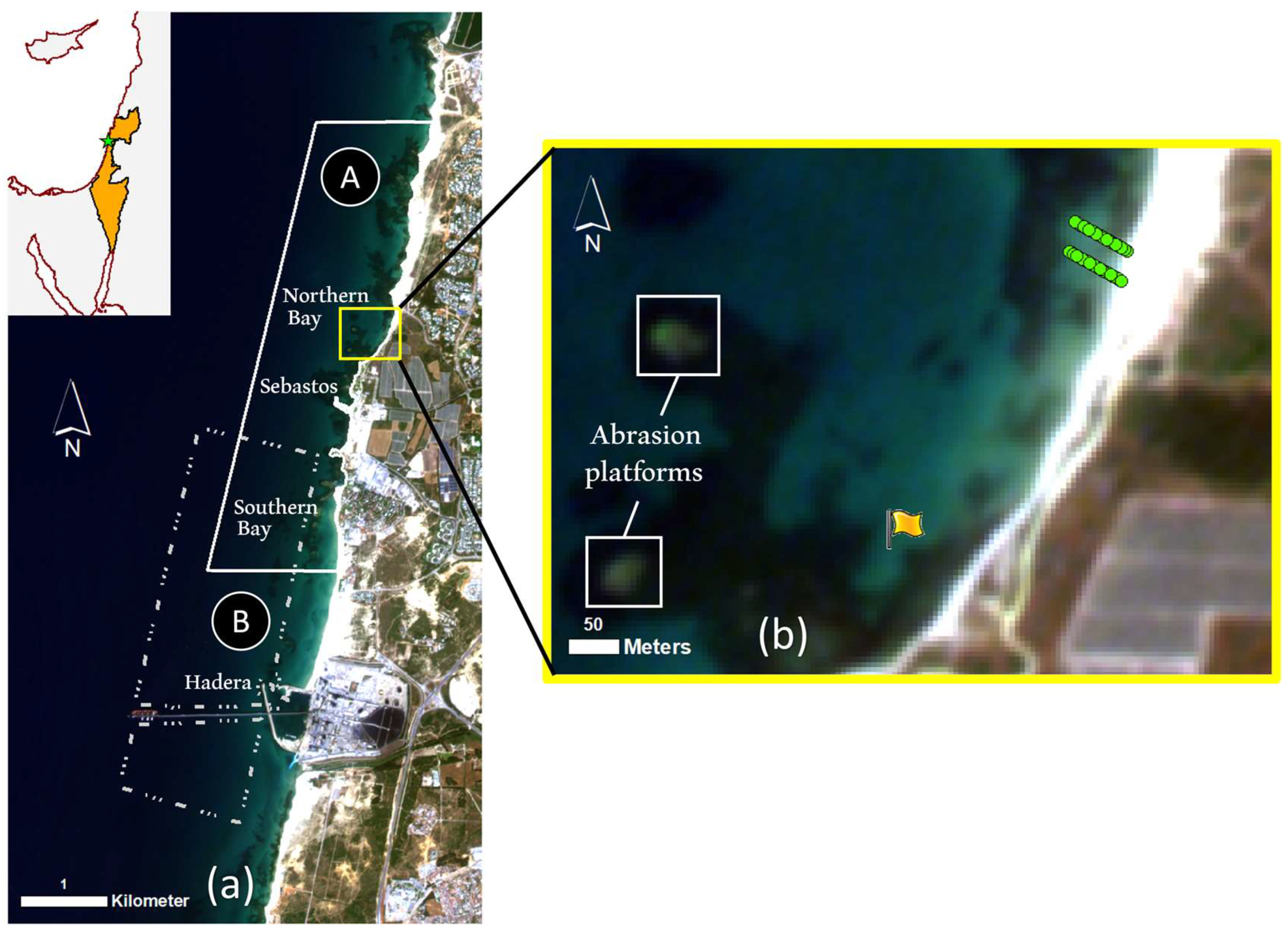
2. Study Area
3. Materials and Methods
3.1. VENμS Satellite Data
3.2. Sonar Data
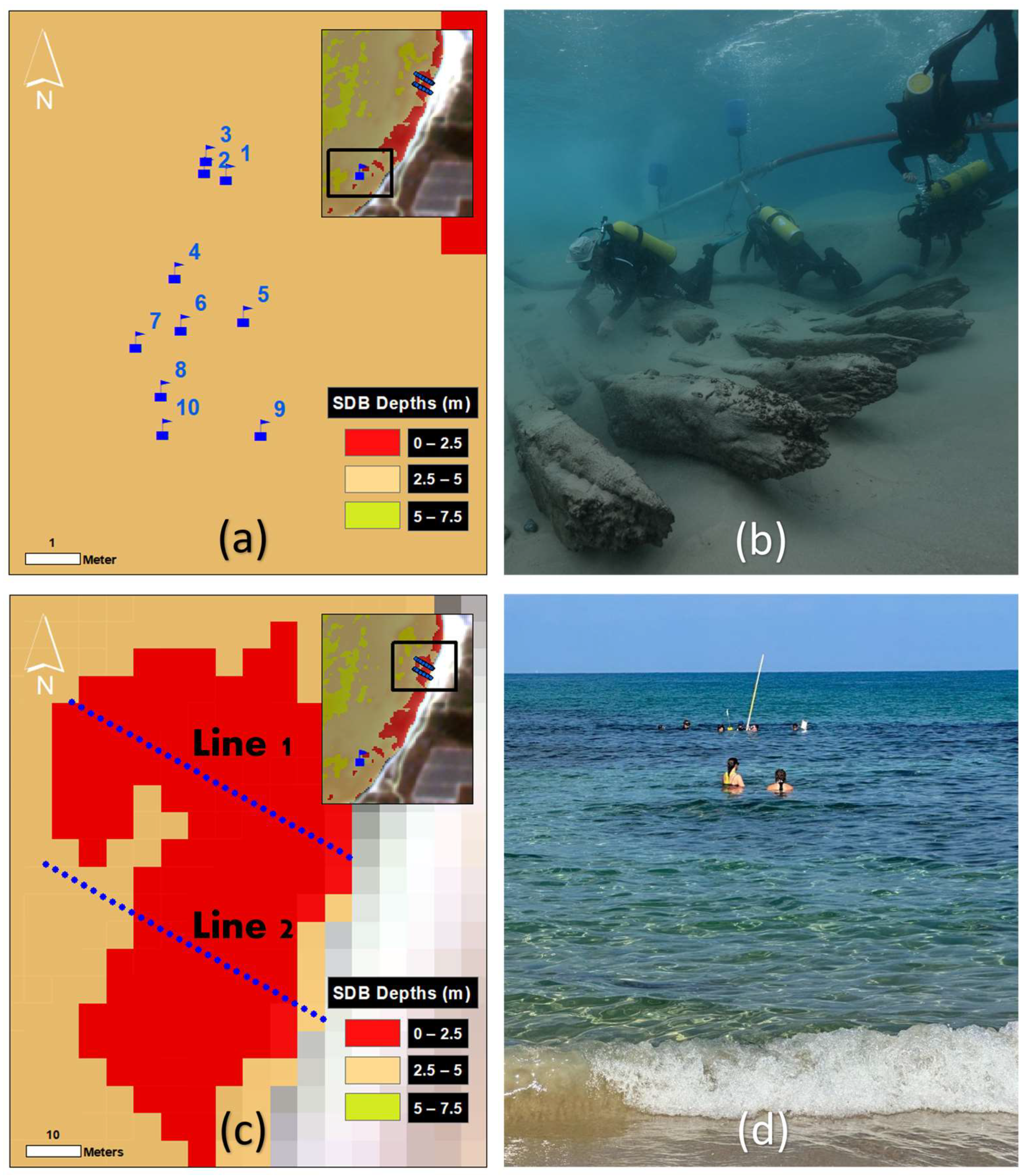
3.3. Ground-Truth Data
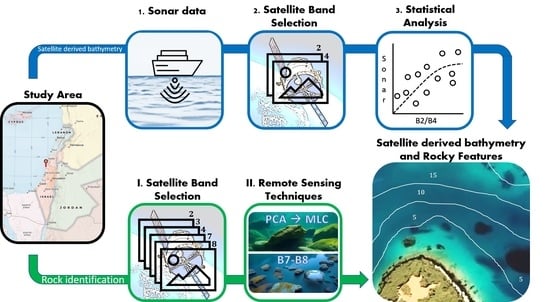
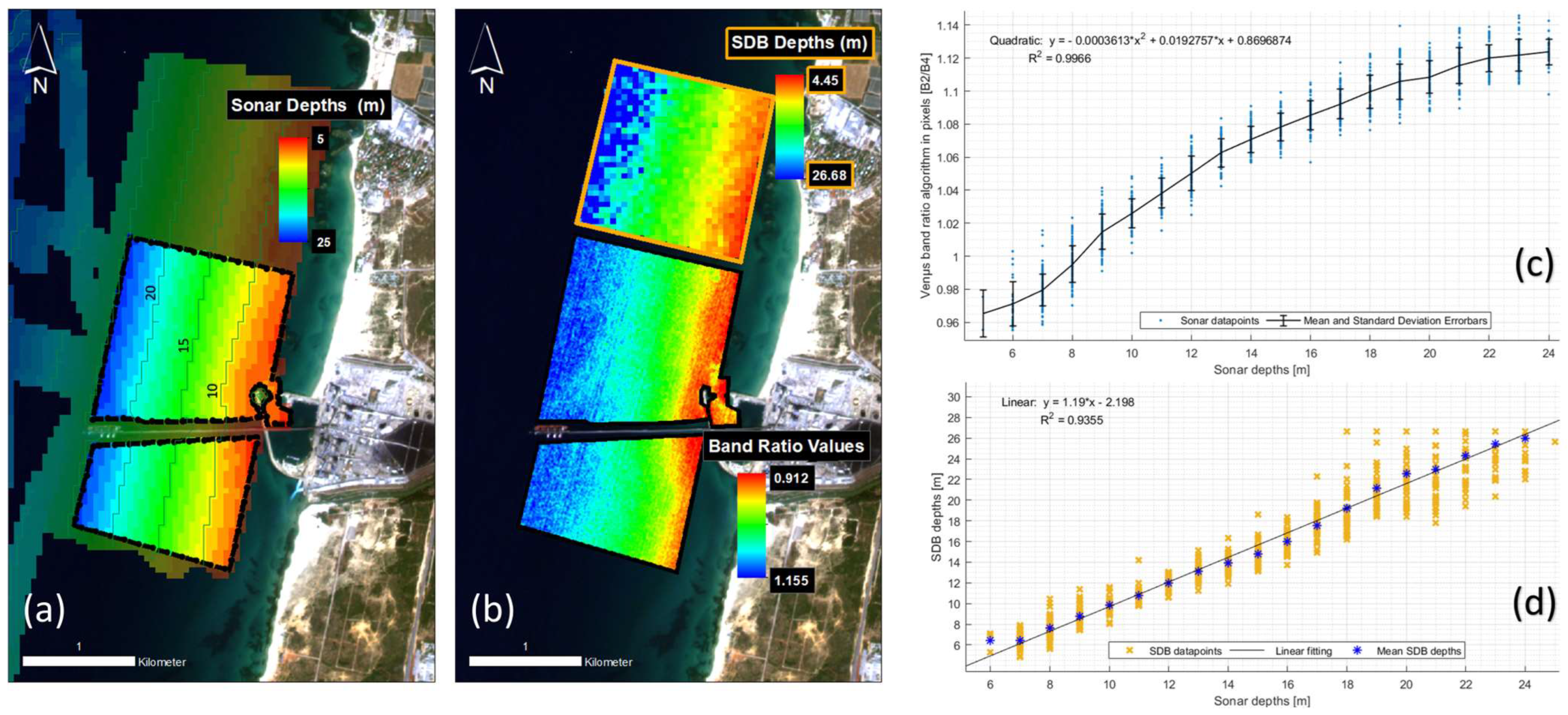
3.4. Empirical Model for SDB Retrieval
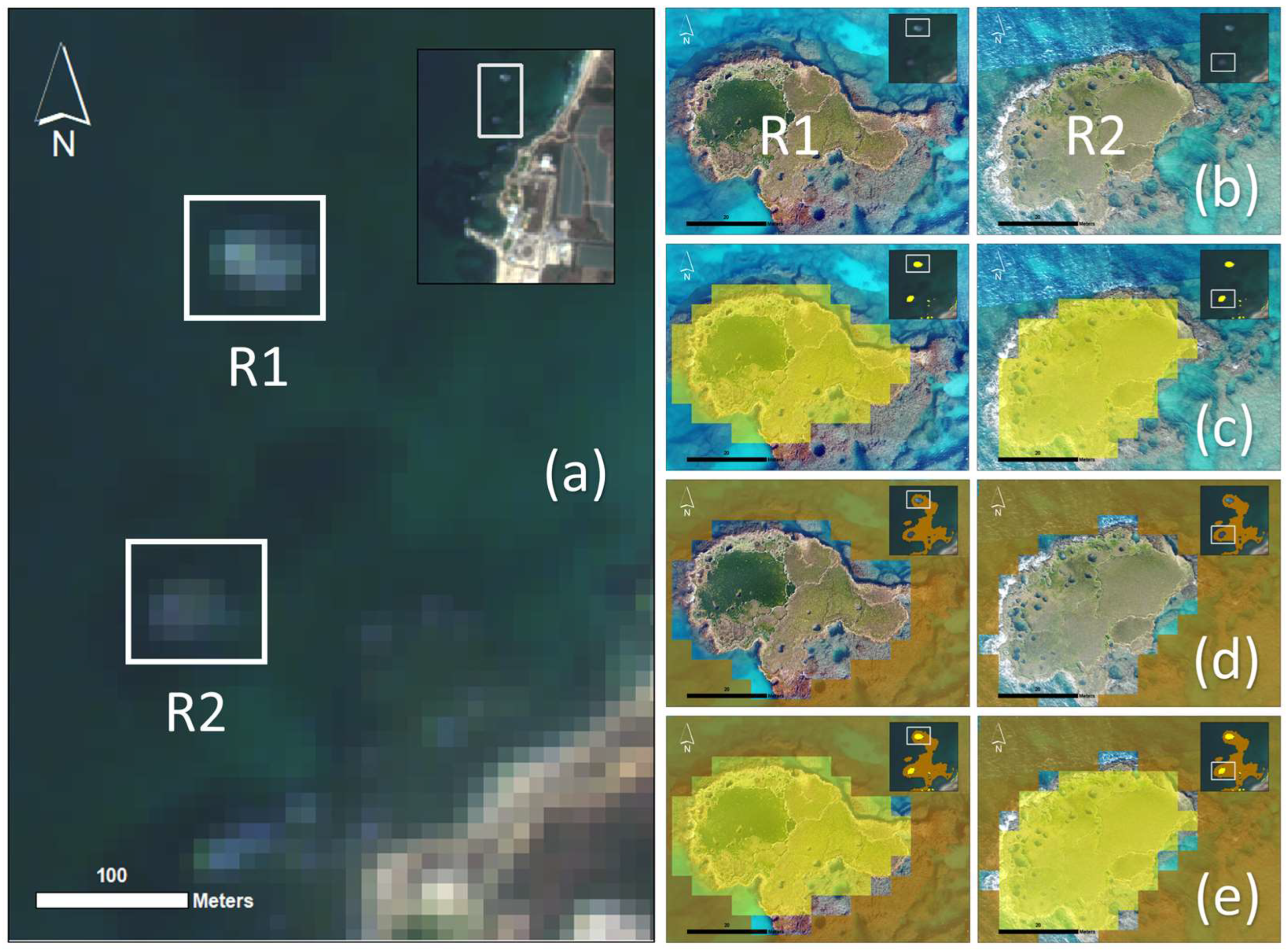
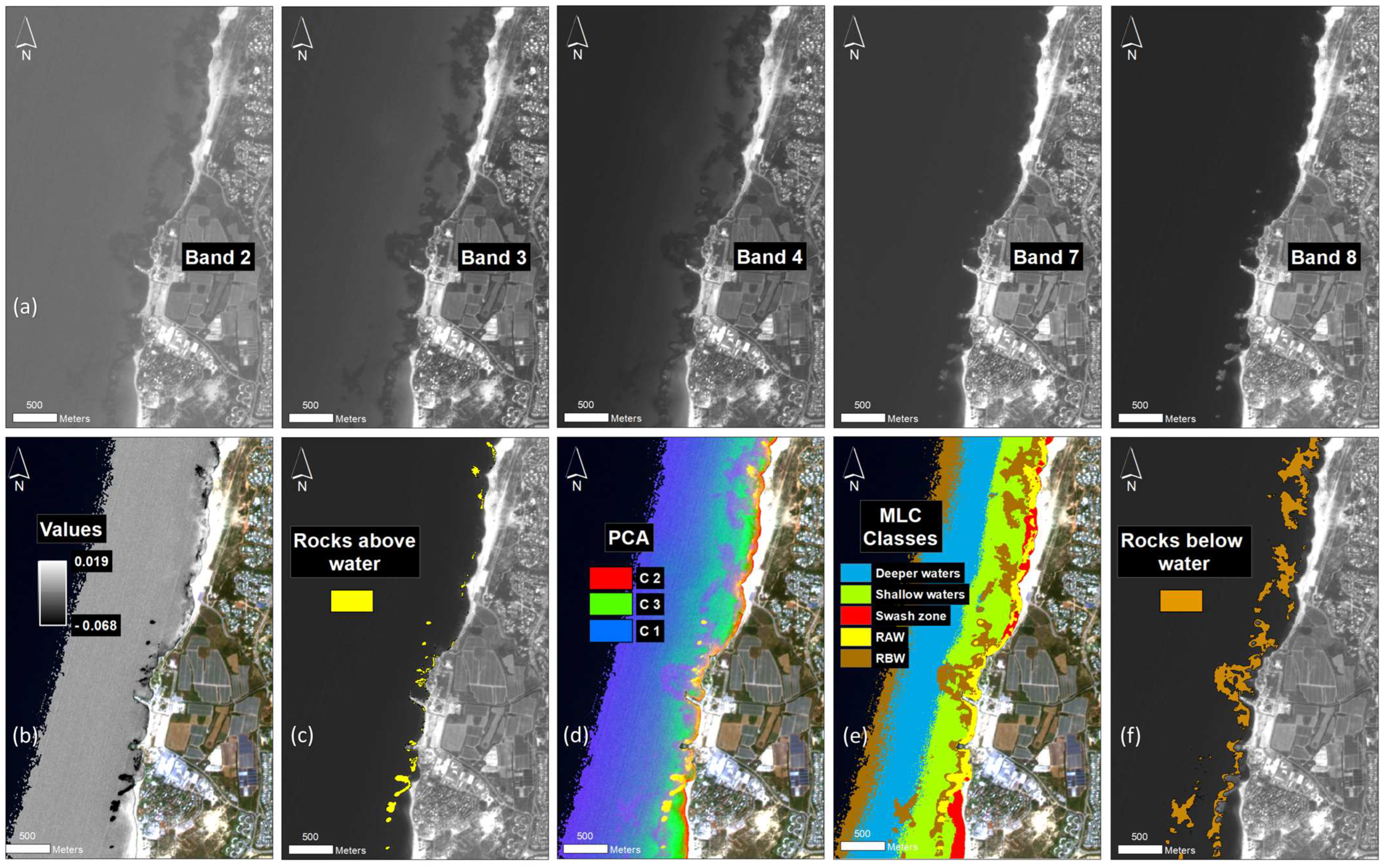
3.5. Satellite-Derived Rock Identification
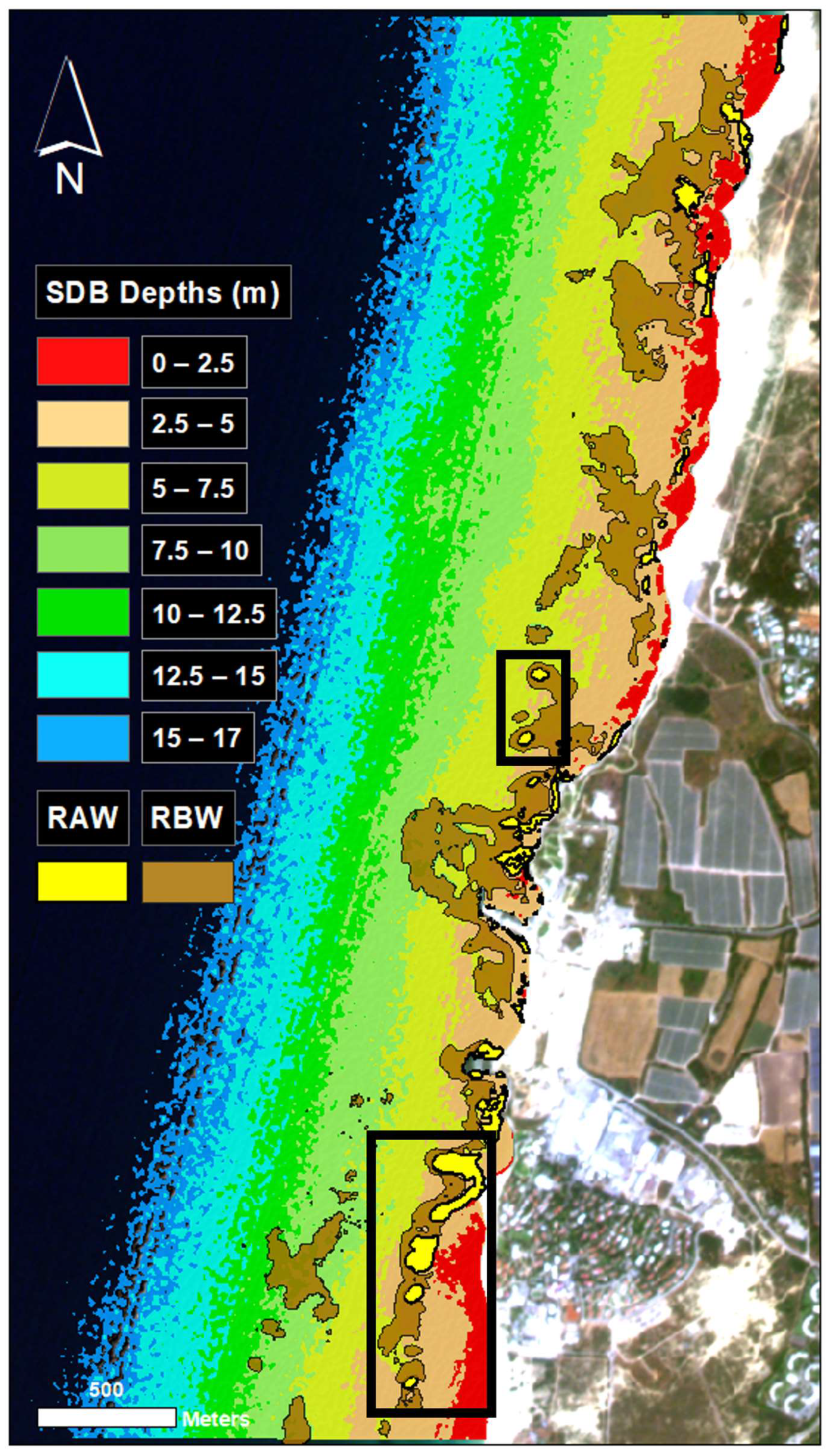
4. Results
5. Discussion
6. Concluding Remarks
Author Contributions
Funding
Data Availability Statement
Acknowledgments
Conflicts of Interest
References
- Smith, M.J.; Pain, C.F. Geomorphological mapping. In The SAGE Handbook of Geomorphology; SAGE Publications Ltd: London, UK, 2011; pp. 142–153. [Google Scholar]
- Elmor, P.; Calder, B.; Petry, F.; Masetti, G.; Yager, R. Aggregation Methods Using Bathymetry Sources of Differing Subjective Reliabilities for Navigation Mapping. Mar. Geod. 2023, 46, 99–128. [Google Scholar]
- Abdullah, M.; Ahmad, S.; Kanwal, A.; Farhan, M.; Saeed, U.B.; Ali, T.; Amin, I. An approach to assess offshore wind power potential using bathymetry and near-hub-height reanalysis data. Ocean Eng. 2023, 280, 114458. [Google Scholar]
- Zaman, H.; Akinturk, A.; Mak, L. Propagation, breaking and interaction of regular and irregular waves over a complex bathymetry with an oil rig. In OCEANS 2021: San Diego—Porto; IEEE: San Diego, CA, USA, 2021; pp. 1–9. [Google Scholar]
- Costa, B.M.; Battista, T.A.; Pittman, S.J. Comparative evaluation of airborne LiDAR and ship-based multibeam SoNAR bathymetry and intensity for mapping coral reef ecosystems. Remote Sens. Environ. 2009, 113, 1082–1100. [Google Scholar] [CrossRef]
- Hedley, J.; Roelfsema, C.; Koetz, B.; Phinn, S. Capability of the Sentinel 2 mission for tropical coral reef mapping and coral bleaching detection. Remote Sens. Environ. 2012, 120, 145–155. [Google Scholar] [CrossRef]
- Pacheco, A.; Horta, J.; Loureiro, C.; Ferreira, Ó. Retrieval of nearshore bathymetry from Landsat 8 images: A tool for coastal monitoring in shallow waters. Remote Sens. Environ. 2015, 159, 102–116. [Google Scholar] [CrossRef]
- Du Bois, P.B. Automatic calculation of bathymetry for coastal hydrodynamic models. Comp. Geosci. 2011, 37, 1303–1310. [Google Scholar] [CrossRef]
- Wedding, L.M.; Friedlander, A.M.; McGranaghan, M.; Yost, R.S.; Monaco, M.E. Using bathymetric lidar to define nearshore benthic habitat complexity: Implications for management of reef fish assemblages in Hawaii. Remote Sens. Environ. 2008, 112, 4159–4165. [Google Scholar] [CrossRef]
- Caston, G.F. Wreck marks: Indicators of net sand transport. Mar. Geol. 1978, 33, 193–204. [Google Scholar] [CrossRef]
- Quinn, R. The role of scour in shipwreck site formation processes and the preservation of wreck-associated scour signatures in the sedimentary record–evidence from seabed and sub-surface data. J. Archaeol. Sci. 2006, 33, 1419–1432. [Google Scholar] [CrossRef]
- Westley, K.; Plets, R.; Quinn, R. Holocene paleo-geographic reconstructions of the Ramore Head area, Northern Ireland, using geophysical and geotechnical data: Paleo-landscape mapping and archaeological implications. Geoarchaeology 2014, 29, 411–430. [Google Scholar] [CrossRef]
- Westley, K. Satellite-derived bathymetry for maritime archaeology: Testing its effectiveness at two ancient harbours in the Eastern Mediterranean. J. Archaeol. Sci. 2021, 38, 8–17. [Google Scholar] [CrossRef]
- Violante, C. Acoustic remote sensing for seabed archaeology. In Proceedings of the International Conference on Metrology for Archaeology and Cultural Heritage, Trento, Italy, 22–24 October 2020; pp. 21–26. [Google Scholar]
- Maarleveld, T.J.; Guérin, U.; Egger, B. Conservation and Site Management. In Manual for Activities Directed at Underwater Cultural Heritage: Guidelines to the Annex of the UNESCO 2001 Convention, 3rd ed.; United Nations Educational, Scientific and Cultural Organization: Paris, France, 2013; pp. 189–192. [Google Scholar]
- Violante, C.; Gallocchio, E.; Pagano, F.; Papadopulos, N. Geophysical and geoarchaeological investigations in the Submerged Archaeological Park of Baia (south Italy). In Proceedings of the IMEKO International Conference on ‘Metrology for Archaeology and Cultural Heritage’, Rome, Italy, 19–21 October 2023; pp. 886–891. [Google Scholar]
- HD-MAX Dual-Frequency Echo Sounder. Available online: https://en.hi-target.com.cn/wp-content/uploads/2022/05/HD-MAX-Brochure-EN-20220513s.pdf (accessed on 3 March 2024).
- D270 SINGLE-BEAM ECHO SOUNDER. Available online: https://chcnav.com/uploads/D270_DS_EN.pdf (accessed on 16 January 2024).
- EM® 2042 Multibeam Echo Sounder for Shallow Waters. Available online: https://www.kongsberg.com/globalassets/discovery/seafloor-mapping/em-multibeams/em-multibeams-media/496233ab_em2042_data_sheet.pdf (accessed on 3 March 2024).
- SeatBat® T50-S SubSea Multibeam Echosounder. Available online: https://www.ashtead-technology.com/wp-content/uploads/2021/06/Teledyne-Reson-SeaBat-T50-S-Multibeam-Echosounder.pdf (accessed on 3 March 2024).
- Szafarczyk, A.; Toś, C. The use of green laser in LiDAR bathymetry: State of the art and recent advancements. Sensors 2012, 23, 292. [Google Scholar] [CrossRef] [PubMed]
- Echo Sounder Combo: ECT D24S Dual-Frequency. Available online: https://shop.sphengineering.com/collections/echosounders/products/ect-d24s-combo (accessed on 3 March 2024).
- Stumpf, R.P.; Holderied, K.; Sinclair, M. Determination of water depth with high-resolution satellite imagery over variable bottom types. Limnol. Oceanogr. 2003, 48, 547–556. [Google Scholar] [CrossRef]
- Lyzenga, D. Remote sensing of bottom reflectance and water attenuation parameters in shallow water using aircraft and Landsat data Remote sensing of bottom reflectance and water attenuation parameters in shallow water using air. Int. J. Remote Sens. 1980, 2, 71–82. [Google Scholar] [CrossRef]
- Dierssen, H.M.; Zimmerman, R.C.; Leathers, R.A.; Downes, T.V.; Davis, C.O. Ocean color remote sensing of seagrass and bathymetry in the Bahamas Banks by high-resolution airborne imagery. Limnol. Oceanogr. 2003, 48, 444–455. [Google Scholar] [CrossRef]
- Evagorou, E.; Argyriou, A.; Papadopoulos, N.; Mettas, C.; Alexandrakis, G.; Hadjimitsis, D. Evaluation of Satellite-Derived Bathymetry from High and Medium-Resolution Sensors Using Empirical Methods. Remote Sens. 2022, 14, 772. [Google Scholar] [CrossRef]
- Hedley, J.D.; Roelfsema, C.; Phinn, S.R. Efficient radiative transfer model inversion for remote sensing applications. Remote Sens. Environ. 2009, 113, 2527–2532. [Google Scholar] [CrossRef]
- Mobley, C.D.; Sundman, L.K.; Davis, C.D.; Bowles, J.H.; Downes, T.V.; Leathers, R.A.; Montes, M.J.; Bisset, W.P.; Kohler, D.D.R.; Reid, R.P.; et al. Interpretation of hyperspectral remote-sensing imagery by spectrum matching and look-up tables. Appl. Opt. 2005, 44, 3576–3591. [Google Scholar] [CrossRef] [PubMed]
- Dekker, A.G.; Phinn, S.R.; Anstee, J.; Bissett, P.; Brando, V.E.; Casey, B.; Fearns, P.; Hedley, J.; Klonowski, W.; Lee, Z.P.; et al. Intercomparison of shallow water bathymetry, hydro-optics, and benthos mapping techniques in Australian and Caribbean coastal environments. Limnol. Oceanogr.-Meth. 2011, 9, 396–425. [Google Scholar] [CrossRef]
- Lee, Z.; Carder, K.L.; Mobley, C.D.; Steward, R.G.; Patch, J.S. Hyperspectral remote sensing for shallow waters: 2. Deriving bottom depths and water properties by optimization. Appl. Opt. 1999, 38, 3831–3843. [Google Scholar] [CrossRef]
- Klonowski, W.M.; Fearns, P.R.; Lynch, M.J. Retrieving key benthic cover types and bathymetry from hyperspectral imagery. J. Appl. Remote Sens. 2007, 1, 011505. [Google Scholar] [CrossRef]
- Wettle, M.; Brando, V.E. Sambuca: Semi-analytical model for bathymetry, unmixing and concentration assessment. Technol. Rep. CSIRO Land Water Sci. Rep. 2006, 22/06, 1–20. [Google Scholar] [CrossRef]
- Collings, S.; Botha, E.J.; Anstee, J.; Campbell, N. Depth from Satellite Images: Depth Retrieval Using a Stereo and Radiative Transfer-Based Hybrid Method. Remote Sens. 2018, 10, 1247. [Google Scholar] [CrossRef]
- Cao, B.; Fang, Y.; Jiang, Z.; Gao, L.; Hu, H. Shallow water bathymetry from WorldView-2 stereo imagery using two-media photogrammetry. Eur. J. Remote Sens. 2019, 52, 506–521. [Google Scholar] [CrossRef]
- Sagawa, T.; Yamashita, Y.; Okumura, T.; Yamanokuchi, T. Satellite Derived Bathymetry Using Machine Learning and Multi-Temporal Satellite Images. Remote Sens. 2019, 11, 1155. [Google Scholar] [CrossRef]
- Dickens, K.; Armstrong, A. Application of Machine Learning in Satellite Derived Bathymetry and Coastline Detection. SMU Data Sci. Rev. 2019, 2, 4. [Google Scholar]
- Tonion, F.; Pirotti, F.; Faina, G.; Paltrinieri, D. A Machine Learning Approach to Multispectral Satellite Derived Bathymetry. ISPRS Ann. Photogramm. Remote Sens. Spat. Inf. Sci. 2020, 3, 565–570. [Google Scholar] [CrossRef]
- Al Najar, M.; Thoumyre, G.; Bergsma, E.W.; Almar, R.; Benshila, R.; Wilson, D.G. Satellite derived bathymetry using deep learning. Mach. Learn. 2021, 112, 1107–1130. [Google Scholar] [CrossRef]
- Li, J.; Yu, Q.; Tian, Y.Q.; Becker, B.L.; Siqueira, P.; Torbick, N. Spatio-temporal variations of CDOM in shallow inland waters from a semi-analytical inversion of Landsat-8. Remote Sens. Environ. 2018, 218, 189–200. [Google Scholar] [CrossRef]
- Gao, J. Bathymetric mapping by means of remote sensing: Methods, accuracy and limitations. Prog. Phys. Geogr. 2009, 33, 103–116. [Google Scholar] [CrossRef]
- Bukata, R.P.; Jerome, J.H.; Kondratyev, A.S.; Pozdnyakov, D.V. Observations of Optical Properties of Natural Waters (The Laurentian Great Lakes). In Optical Properties and Remote Sensing of Inland and Coastal Waters, 1st ed.; CRC Press: Boca Raton, FL, USA, 1995; pp. 183–190. [Google Scholar]
- Kao, H.M.; Ren, H.; Lee, C.S.; Chang, C.P.; Yen, J.Y.; Lin, T.H. Determination of shallow water depth using optical satellite images. Int. J. Remote Sens. 2009, 30, 6242. [Google Scholar] [CrossRef]
- Mavraeidopoulos, A.K.; Pallikaris, A.; Oikonomou, E. Satellite derived bathymetry (SDB) and safety of navigation. Int. Hydrogr. Rev. 2017, 71, 7–20. [Google Scholar]
- Dewi, R.S.; Sofian, I. The application of satellite derived bathymetry for coastline mapping. IOP Conf. Ser. Earth Environ. Sci. 2022, 950, 012088. [Google Scholar] [CrossRef]
- Ashphaq, M.; Srivastava, P.K.; Mitra, D. Review of near-shore satellite derived bathymetry: Classification and account of five decades of coastal bathymetry research. J. Ocean Eng. Sci. 2021, 6, 340–359. [Google Scholar] [CrossRef]
- Guzinski, R.; Spondylis, E.; Michalis, M.; Tusa, S.; Brancato, G.; Minno, L.; Hansen, L.B. Exploring the utility of bathymetry maps derived with multispectral satellite observations in the field of underwater archaeology. Open Archaeol. 2016, 2, 243–246. [Google Scholar] [CrossRef]
- Lassak, D.; Novikova, A.; Argyriou, A.V.; Papadopoulos, N. Satellite Derived Bathymetry for the Islands of South Eastern Crete. In Proceedings of the IMEKO International Conference on ‘Metrology for Archaeology and Cultural Heritage’, Rome, Italy, 19–21 October 2023. [Google Scholar]
- Final Report Summary—ITACA (Innovation Technologies and Applications for Coastal Archaeological Sites). Available online: https://cordis.europa.eu/project/id/606805 (accessed on 9 February 2024).
- VENμS Mission and Products. VENμS Vegetation and Environment Monitoring New Micro Satellite. Available online: https://venus.bgu.ac.il/Links/VENuS_mission_summary_VM05_v02.pdf (accessed on 23 March 2023).
- CNES. Joint French-Israeli Venus Mission. Available online: https://cnes.fr/en/web/CNES-en/3766-joint-french-israeli-vens-mission.php (accessed on 26 July 2021).
- VM05 MISSION (Updated on 20th October 2023). Available online: https://venus.bgu.ac.il/venus/ (accessed on 7 March 2024).
- Raban, A.; Artzy, M.; Goodman, B.; Gal, Z. The Harbour of Sebastos (Caesarea Maritima) in its Roman Mediterranean Context; Archaeopress: Oxford, UK, 2009; pp. 69–149. [Google Scholar]
- Bergin, B. The Innovative Genius of Herod at Caesarea Maritima. Cult. Relig. 2018, 6, 377–391. [Google Scholar]
- Raban, A.J. Underwater Excavations in the Herodian Harbor Sebastos, 1995–1999 Seasons; BAR Int. Series: Oxford, UK, 2008; Volume 1784, pp. 129–142. [Google Scholar]
- Galili, E.; Salamon, A.; Gambash, G.; Zviely, D. Archaeological and Natural Indicators of Sea-Level and Coastal Changes: The Case Study of the Caesarea Roman Harbor. Geosciences 2021, 11, 306. [Google Scholar] [CrossRef]
- Boyce, J.I.; Reinhardt, E.G.; Raban, A.; Pozza, M.R. Marine magnetic survey of a submerged Roman harbour, Caesarea Maritima, Israel. Int. J. Naut. Archaeol. 2004, 33, 122–136. [Google Scholar] [CrossRef]
- Ratzlaff, A.; Galili, E.; Waiman-Barak, P.; Yasur-Landau, A. The Plurality of Harbors at Caesarea: The Southern Anchorage in Late Antiquity. J. Marit. Archaeol. 2017, 12, 125–146. [Google Scholar] [CrossRef]
- Galili, E.; Dahari, U.; Shanit, J. Underwater surveys and rescue excavations along the Israeli coast. Int. J. Naut. Archaeol. 1993, 22, 61–77. [Google Scholar] [CrossRef]
- Kidson, C. Sea-Level Changes in the Holocene. In Sea-Level Research: A Manual for Collection and Evaluation of Data; van de Plassche, O., Ed.; Geo Books: Norwich, UK, 1986; pp. 27–64. [Google Scholar]
- MarineTraffic. Available online: https://www.marinetraffic.com/en/ais/details/ships/shipid:7059908/mmsi:428003005/imo:0/vessel:HADERA_PORT (accessed on 27 May 2023).
- Shipnext. Available online: https://shipnext.com/port/hadera-ilhad-isr (accessed on 27 July 2023).
- Raban, A. Sebastos: The Royal Harbour at Caesarea Maritima—A Short-Lived Giant. Int. J. Naut. Archaeol. 1992, 21, 111–124. [Google Scholar] [CrossRef]
- Gvirtzman, Z.; Reshef, M.; Buch-Leviatan, O.; Groves-Gidney, G.; Karcz, Z.; Makovsky, Y.; Ben-Avraham, Z. Bathymetry of the Levant basin: Interaction of salt-tectonics and surficial mass movements. Mar. Geol. 2015, 360, 25–39. [Google Scholar] [CrossRef]
- EM 1002—Multibeam Echo Sounder. Available online: http://linux.geodatapub.com/shipwebpages/survey%20gear/Multibeam/EM1002%20-%20Powell/M%201002%20Product%20Description.pdf (accessed on 14 February 2024).
- Seabeam 3050 N at a Glance. Available online: https://www.yumpu.com/en/document/read/27114766/seabeam-3050-n-elac-nautik/4 (accessed on 15 February 2024).
- Bowens, A. Underwater Archaeology: The NAS Guides to Principles and Practice, 2nd ed.; John Wiley & Sons Ltd.: Wests Sussex, UK, 2009; p. 92. [Google Scholar]
- Traganos, D.; Poursanidis, D.; Aggarwal, B.; Chrysoulakis, N.; Reinartz, P. Estimating satellite-derived bathymetry (SDB) with the google earth engine and sentinel-2. Remote Sens. 2018, 10, 859. [Google Scholar] [CrossRef]
- Jagalingam, P.; Akshaya, B.J.; Hegde, A.V. Bathymetry Mapping Using Landsat 8 Satellite Imagery. Procedia Eng. 2015, 116, 560–566. [Google Scholar] [CrossRef]
- Li, J.; Knapp, D.E.; Lyons, M.; Roelfsema, C.; Phinn, S.; Schill, S.R.; Asner, G.P. Automated Global Shallow Water Bathymetry Mapping Using Google Earth Engine. Remote Sens. 2021, 13, 1469. [Google Scholar] [CrossRef]
- Resample (Data Management). Available online: https://pro.arcgis.com/en/pro-app/latest/tool-reference/data-management/resample.htm (accessed on 19 February 2024).
- Amante, C.J.; Eakins, B.W. Accuracy of interpolated bathymetry in digital elevation 657 models. J. Coast. Res. 2016, 76, 123–133. [Google Scholar] [CrossRef]
- Conger, C.L.; Hochberg, E.J.; Fletcher, C.H.; Atkinson, M.J. Decorrelating remote sensing color bands from bathymetry in optically shallow waters. IEEE Tran. Geosci. Remote Sens. 2006, 44, 1655–1660. [Google Scholar] [CrossRef]
- Gao, B.C. NDWI—A normalized difference water index for remote sensing of vegetation liquid water from space. Remote Sens. Environ. 1996, 58, 257–266. [Google Scholar] [CrossRef]
- Li, J.; Knapp, D.E.; Schill, S.R.; Roelfsema, C.; Phinn, S.; Silman, M.; Asner, G.P. Adaptive bathymetry estimation for shallow coastal waters using Planet Dove satellites. Remote Sens. Environ. 2019, 232, 111302. [Google Scholar] [CrossRef]
- Rosen, D.S. A Review of Sea Level Monitoring Status in Israel. In Proceedings of the Intergovernmental Oceanographic Commission & International Commission for the Scientific Exploration of the Mediterranean Sea MedGLOSS Pilot Network Workshop and Coordination Meeting, Haifa, Israel, 15–17 May 2000; Volume 4. [Google Scholar]
- Nantet, E. Phortia: Le Tonnage des Navires de Commerce en Méditerranée: Du Viiie Siècle av. L’ère Chrétienne au Viie Siècle de L’ère Chrétienne; Presses Universitaires de Rennes: Rennes, France, 2016; p. 226. [Google Scholar]


| Bands | λ Min (nm) | λ Max (nm) | λ Central (nm) | Bandwidth |
|---|---|---|---|---|
| B1 | 383.9 | 463.9 | 423.9 | 40 |
| B2 | 406.9 | 486.9 | 446.9 | 40 |
| B3 | 451.9 | 531.9 | 491.9 | 40 |
| B4 | 515 | 595 | 555 | 40 |
| B5 | 579.7 | 659.7 | 619.7 | 40 |
| B6 | 589.5 | 649.5 | 619.7 | 40 |
| B7 | 636.2 | 696.2 | 666.2 | 40 |
| B8 | 678 | 726 | 702 | 30 |
| B9 | 725.1 | 757.1 | 741.1 | 24 |
| B10 | 766.2 | 798.2 | 782.2 | 16 |
| B11 | 821.1 | 901.1 | 861.1 | 40 |
| B12 | 888.7 | 928.7 | 908.7 | 20 |
| Sonar Depth (m) | Mean SDB Values (m) | Std Dev. SDB Values (m) | Diff. in Percentage (%) | Depth Difference (m) |
|---|---|---|---|---|
| 6 | 6.407 | 0.990 | 6.783 | 0.407 |
| 7 | 6.414 | 0.791 | 8.371 | −0.586 |
| 8 | 7.662 | 0.955 | 4.225 | −0.338 |
| 9 | 8.758 | 0.821 | 2.689 | −0.242 |
| 10 | 9.812 | 0.731 | 1.880 | −0.188 |
| 11 | 10.762 | 0.726 | 2.164 | −0.238 |
| 12 | 11.995 | 0.669 | 0.042 | −0.005 |
| 13 | 13.098 | 0.836 | 0.754 | 0.098 |
| 14 | 13.909 | 0.828 | 0.650 | −0.091 |
| 15 | 14.781 | 0.997 | 1.460 | −0.219 |
| 16 | 16.018 | 1.081 | 0.113 | 0.018 |
| 17 | 17.548 | 1.356 | 3.224 | 0.548 |
| 18 | 19.200 | 2.368 | 6.667 | 1.200 |
| 19 | 21.157 | 2.162 | 11.353 | 2.157 |
| 20 | 22.581 | 2.694 | 12.905 | 2.581 |
| 21 | 22.973 | 3.051 | 9.395 | 1.973 |
| 22 | 24.312 | 2.425 | 10.509 | 2.312 |
| 23 | 25.449 | 1.803 | 10.648 | 2.449 |
| 24 | 25.975 | 1.399 | 8.229 | 1.975 |
| RMSE [6–17 m] = 0.949 m RMSE [6–24 m] = 2.037 m | ||||
| ID | Shipwreck’s Hull (m) | SDB (m) | Diff. (%) | ID | Line 1 (m) | SDB (m) | Diff. (%) | Line 2 (m) | SDB (m) | Diff. (%) |
|---|---|---|---|---|---|---|---|---|---|---|
| 1 | 0.385 | 2.017 | 423.896 | 0.42 | 2.52 | 500.000 | ||||
| 1 | 2.544 | 2.604 | 2.358 | 2 | 0.6 | 2.017 | 236.167 | 0.65 | 2.52 | 287.692 |
| 3 | 0.83 | 2.017 | 143.012 | 0.83 | 2.52 | 203.614 | ||||
| 4 | 1.06 | 1.754 | 65.472 | 1.03 | 2.323 | 125.534 | ||||
| 2 | 2.577 | 2.604 | 1.048 | 5 | 1.145 | 1.754 | 53.188 | 1.17 | 2.323 | 98.547 |
| 6 | 1.355 | 1.859 | 37.196 | 1.31 | 2.323 | 77.328 | ||||
| 7 | 1.489 | 1.928 | 29.483 | 1.44 | 2.195 | 52.431 | ||||
| 3 | 2.798 | 2.604 | 6.934 | 8 | 1.589 | 1.928 | 21.334 | 1.54 | 2.264 | 47.013 |
| 9 | 1.691 | 1.928 | 14.015 | 1.58 | 2.195 | 38.924 | ||||
| 10 | 1.7 | 2.188 | 28.706 | 1.64 | 2.107 | 28.476 | ||||
| 4 | 2.665 | 2.579 | 3.227 | 11 | 1.656 | 2.188 | 32.126 | 1.67 | 2.107 | 26.168 |
| 12 | 1.73 | 2.188 | 26.474 | 1.8 | 2.107 | 17.056 | ||||
| 13 | 1.79 | 2.155 | 20.391 | 1.72 | 1.981 | 15.174 | ||||
| 5 | 2.523 | 2.579 | 2.220 | 14 | 1.78 | 2.321 | 30.393 | 1.91 | 1.983 | 3.822 |
| 15 | 1.815 | 2.321 | 27.879 | 2.72 | 1.983 | 27.096 | ||||
| 16 | 1.635 | 2.248 | 37.492 | 2.185 | 2.169 | 0.732 | ||||
| 6 | 2.852 | 2.579 | 9.572 | 17 | 1.875 | 2.248 | 19.893 | 2.25 | 2.426 | 7.822 |
| 18 | 1.85 | 2.317 | 25.243 | 2.29 | 2.169 | 5.284 | ||||
| 19 | 1.95 | 2.286 | 17.231 | 2.26 | 2.576 | 13.982 | ||||
| 7 | 2.809 | 2.633 | 6.266 | 20 | 1.925 | 2.317 | 20.364 | 2.28 | 2.481 | 8.816 |
| 21 | 1.935 | 2.28 | 17.829 | 2.28 | 2.426 | 6.404 | ||||
| 22 | 1.65 | 2.26 | 36.970 | 2.32 | 2.576 | 11.034 | ||||
| 8 | 2.548 | 2.663 | 4.513 | 23 | 1.55 | 2.286 | 47.484 | 2.37 | 2.576 | 8.692 |
| 24 | 1.17 | 2.286 | 95.385 | 2.36 | 2.576 | 9.153 | ||||
| 25 | 2.17 | 2.284 | 5.253 | 2.02 | 2.77 | 37.129 | ||||
| 9 | 2.178 | 2.579 | 18.411 | 26 | 2.05 | 2.189 | 6.780 | 1.615 | 2.56 | 58.514 |
| 27 | 2.37 | 2.189 | 7.637 | 2.795 | 2.56 | 8.408 | ||||
| 28 | 2.01 | 2.285 | 13.682 | 2.645 | 2.77 | 4.726 | ||||
| 10 | 2.770 | 2.633 | 4.946 | 29 | 2.4 | 2.285 | 4.792 | 2.71 | 2.9 | 7.011 |
| 30 | 2.4 | 2.558 | 6.583 | 1.72 | 2.77 | 61.047 |
| Statistics | Shipwreck’s Hull (10 Points) | Line 1 (30 Points) | Line 2 (30 Points) | All Measurements (70 Points) |
|---|---|---|---|---|
| Mean (m) | 0.513 | 0.531 | 0.615 | 0.513 |
| Std Dev. (m) | 0.109 | 0.364 | 0.55 | 0.46 |
| RMSE (m) | 0.187 | 0.643 | 0.825 | 0.688 |
Disclaimer/Publisher’s Note: The statements, opinions and data contained in all publications are solely those of the individual author(s) and contributor(s) and not of MDPI and/or the editor(s). MDPI and/or the editor(s) disclaim responsibility for any injury to people or property resulting from any ideas, methods, instructions or products referred to in the content. |
© 2024 by the authors. Licensee MDPI, Basel, Switzerland. This article is an open access article distributed under the terms and conditions of the Creative Commons Attribution (CC BY) license (https://creativecommons.org/licenses/by/4.0/).
Share and Cite
Diaz, G.; Lehahn, Y.; Nantet, E. Satellite-Derived Bathymetry in Support of Maritime Archaeological Research—VENμS Imagery of Caesarea Maritima, Israel, as a Case Study. Remote Sens. 2024, 16, 1218. https://doi.org/10.3390/rs16071218
Diaz G, Lehahn Y, Nantet E. Satellite-Derived Bathymetry in Support of Maritime Archaeological Research—VENμS Imagery of Caesarea Maritima, Israel, as a Case Study. Remote Sensing. 2024; 16(7):1218. https://doi.org/10.3390/rs16071218
Chicago/Turabian StyleDiaz, Gerardo, Yoav Lehahn, and Emmanuel Nantet. 2024. "Satellite-Derived Bathymetry in Support of Maritime Archaeological Research—VENμS Imagery of Caesarea Maritima, Israel, as a Case Study" Remote Sensing 16, no. 7: 1218. https://doi.org/10.3390/rs16071218
APA StyleDiaz, G., Lehahn, Y., & Nantet, E. (2024). Satellite-Derived Bathymetry in Support of Maritime Archaeological Research—VENμS Imagery of Caesarea Maritima, Israel, as a Case Study. Remote Sensing, 16(7), 1218. https://doi.org/10.3390/rs16071218