Abstract
Single Image Super-Resolution (SISR) for image enhancement enables the generation of high spatial resolution in Remote Sensing (RS) images without incurring additional costs. This approach offers a practical solution to obtain high-resolution RS images, addressing challenges posed by the expense of acquisition equipment and unpredictable weather conditions. To address the over-smoothing of the previous SISR models, the diffusion model has been incorporated into RS SISR to generate Super-Resolution (SR) images with enhanced textural details. In this paper, we propose a Diffusion model with Adversarial Learning Strategy (DiffALS) to refine the generative capability of the diffusion model. DiffALS integrates an additional Noise Discriminator (ND) into the training process, employing an adversarial learning strategy on the data distribution learning. This ND guides noise prediction by considering the general correspondence between the noisy image in each step, thereby enhancing the diversity of generated data and the detailed texture prediction of the diffusion model. Furthermore, considering that the diffusion model may exhibit suboptimal performance on traditional pixel-level metrics such as Peak Signal-to-Noise Ratio (PSNR) and Structural Similarity (SSIM), we showcase the effectiveness of DiffALS through downstream semantic segmentation applications. Extensive experiments demonstrate that the proposed model achieves remarkable accuracy and notable visual enhancements. Compared to other state-of-the-art methods, our model establishes an improvement of 189 for Fréchet Inception Distance (FID) and 0.002 for Learned Perceptual Image Patch Similarity (LPIPS) in a SR dataset, namely Alsat, and achieves improvements of 0.4%, 0.3%, and 0.2% for F1 score, MIoU, and Accuracy, respectively, in a segmentation dataset, namely Vaihingen.
1. Introduction
Enhancements in satellite technologies have greatly expanded the applications of Remote Sensing (RS) imagery in areas such as disaster relief, geology, environment, and engineering construction [1,2,3,4]. Despite these advancements, challenges persist due to limitations in imaging instruments and long-range shooting, resulting in RS satellite images with resolutions that cannot fully meet the requirements for downstream applications, especially on semantic segmentation tasks [5,6]. In contrast to focusing solely on equipment improvement, the Single-Image Super-Resolution (SISR) [7,8,9,10] technique at the sub-pixel level is a more cost-effective strategy. It could improve the resolution by accurately representing the information already present in the images. In contrast to natural images, satellite images capture surface details across wide areas with lower resolution and often contain multispectral data. Consequently, Super-Resolution (SR) models tailored for remote sensing prioritize effectively handling minor objects based on optical or multispectral information. Recent advancements in deep-learning (DL) methods [11,12,13] for SISR have demonstrated superior performance compared to traditional approaches. These DL methods can be categorized into three groups: Convolutional Neural Network (CNN)-based models, Generative Adversarial Network (GAN)-based methods [14], and diffusion-based methods [15].
As the pioneering models in DL, CNN-based models [16,17,18,19,20] serve as baseline models that generate SR images in an end-to-end manner. They are trained by minimizing the difference between the SR and High-Resolution (HR) images. Notably, VDSR [21] was groundbreaking in utilizing deep networks for effective feature expansion. Given the potency of deep networks, several models incorporating residual learning [22,23] and multiscale architecture [24,25] have been introduced to address the challenges associated with training exceptionally deep networks. In the realm of RS, Feng et al. [26] developed a lightweight CNN structure to enhance hierarchical feature learning and extract feature representations. More recently, with the advent of the Transformer architecture, several CNN-based models have integrated self-attention modules to facilitate global information extraction. Both ESRT [27] and Interactformer [28] have adopted a hybrid model structure, incorporating a CNN branch and a Transformer branch. This design aims to extract deep features and address long-distance dependencies between similar local regions. Despite these advancements, a notable limitation of CNN-based models arises from their primary training strategy, which minimizes differences between SR and HR images with metrics such as Peak Signal-to-Noise Ratio (PSNR) and Structural Similarity (SSIM) at the pixel level. This limitation becomes evident in the persistent issue of over-smoothing, as metrics like PSNR and SSIM tend to favor images with high smoothness, lacking detailed texture, over sharper images with more texture predictions.
To address the limitations of CNN-based models, GAN-based models, a kind of generative model, have been introduced with a novel generator-discriminator training approach. This approach enables GAN-based models to improve the SR image quality with the additional loss function determined by the discriminator instead of merely minimizing pixel differences between SR and HR images. The RS methods like MA-GAN [29] and RRSGAN [30] have demonstrated quality improvements in the human judgment of GAN-based models. However, it is crucial to note that the GAN-based models still heavily rely on pixel-level loss, and the perceptual loss is only one aspect of the models’ training guidance, limiting their advantages. Additionally, GAN-based models continue to face challenges [31], including instability and model collapse issues, as highlighted in previous studies.
A cutting-edge generative model, diffusion model [15], has garnered significant attention, particularly in various computer vision tasks, with a notable emphasis on conditional image generation. This model excels in producing images of high perceptual quality with detailed texture generation, aligning well with the requirements of the SISR field. Diverging from CNN-based and GAN-based models, the diffusion model focuses on learning the data distribution rather than the feature mapping between LR and HR images. This unique approach enables the diffusion model to restore images based on specified conditions from random Gaussian noise images, showcasing its flexibility and effectiveness. Early achievements in the SR task, such as SR3 [32] and SRDiff [33], represent notable applications of the diffusion model. In the domain of RS, EDiffSR [34] leveraged the diffusion architecture and achieved commendable noise prediction performance through simplified channel attention and straightforward gate operations, significantly reducing computational costs. EHC-DMSR [35] introduced a Fourier high-frequency spatial constraint to emphasize high-frequency spatial loss and optimize the reverse diffusion direction.
In this paper, as the adversarial learning strategy has demonstrated the ability to enhance data diversity and texture prediction in GAN-based models, we propose a novel diffusion model with Adversarial Learning Strategy (DiffALS) to RS SISR. With the highly detailed texture requirement of the RS SR task, DiffALS integrates an adversarial learning strategy into the diffusion framework to further stimulate the detailed texture generation capability of the diffusion model. Specifically, we employ a Noise Discriminator (ND) to introduce an additional adversarial loss by evaluating whether the given is real or fake during the training process. The pairs of real , real and real , fake are input into the discriminator for training and loss generation. The fake is calculated through the real and the predicted noise, while the real and are sampled from , which are real noising images, where T is the total number of diffusion steps. This adversarial learning strategy improves the data diversity generated by the diffusion model and contributes to a more nuanced and detailed texture generation by considering the general correspondence between the whole noising image contents, and . In addition, recognizing the limitations of traditional metrics like PSNR and SSIM, particularly when dealing with SR tasks with high magnification factors, we adopt a novel evaluation approach. To demonstrate that our method truly improves the image quality and accuracy instead of just a hallucination for human perception, we leverage the downstream semantic segmentation task, utilizing SR images’ performance in semantic segmentation to evaluate the models. This work provides a more meaningful evaluation metric to prove that our model surpasses its baseline SRDiff method and other comparable methods in terms of visual quality and performance in semantic segmentation. The main contributions of this work can be summarized as follows.
- We introduce a novel approach named Diffusion model with Adversarial Learning Strategy (DiffALS), which integrates the ND network into the diffusion training process. The additional adversarial loss generated by the ND network takes into account the relationship between adjacent noisy images, thereby guiding the training of the CNP and fully leveraging image content information. This guidance from the ND network enhances the detailed texture generation capability in the diffusion model;
- To assess the model’s performance fairly, the experiment results on semantic segmentation are introduced to evaluate the model performance. We utilize a pre-trained model to perform semantic segmentation on the enhanced SR images generated by different models. The model’s effectiveness can be further demonstrated by its superior suitability in image-related applications, considering the diverse feedback from existing matrices;
- Extensive experiments on three RS datasets, including two SR datasets, namely OLI2MSI, Alsat, and a segmentation dataset, namely Vaihingen, confirm the superior performance of the proposed method on the SR task and its downstream application as compared to the state-of-the-art methods.
2. Methods
2.1. DiffALS Architecture
As shown in Figure 1, the architecture of DiffALS is built upon the diffusion model, which can be partitioned into two Markovian processes: the forward process and the reverse process.

Figure 1.
The forward and reverse process of DiffALS.
2.1.1. Forward Process
During the forward process, Gaussian noise is applied to the HR images, transforming the data distribution into the latent variable distribution.
where and are the Gaussian distribution and the identity matrix, respectively. is a set of hyper-parameters that determine the strength of the noise added at each iteration. For simplicity, we denote and . The conditional distribution of based on is
As a result, each can be calculated based on directly with the following formula:
where means an all-zero matrix.
2.1.2. Reverse Process
The reverse process involves eliminating noise from a noisy image and reverting the latent variable distribution back to the data distribution. A network parameterized by is trained to approximate the reverse process distribution.
where and are the mean and variance of the distribution on t step.
In order to determine the mean and variance, the evidence lower bound (ELBO) on the log-likelihood, KL divergence, and variance reduction are applied.
For simplicity, the loss function of the diffusion process minimizes the difference between the random initiated noise and the predicted noise :
where is the predicted noise generated by the network. As a result, the network is named Conditional Noise Predictor (CNP).
Finally, the formula of calculated based on and is given by
where is the variance of the Gaussian distribution in t diffusion step.
2.2. Conditional Noise Predictor (CNP)
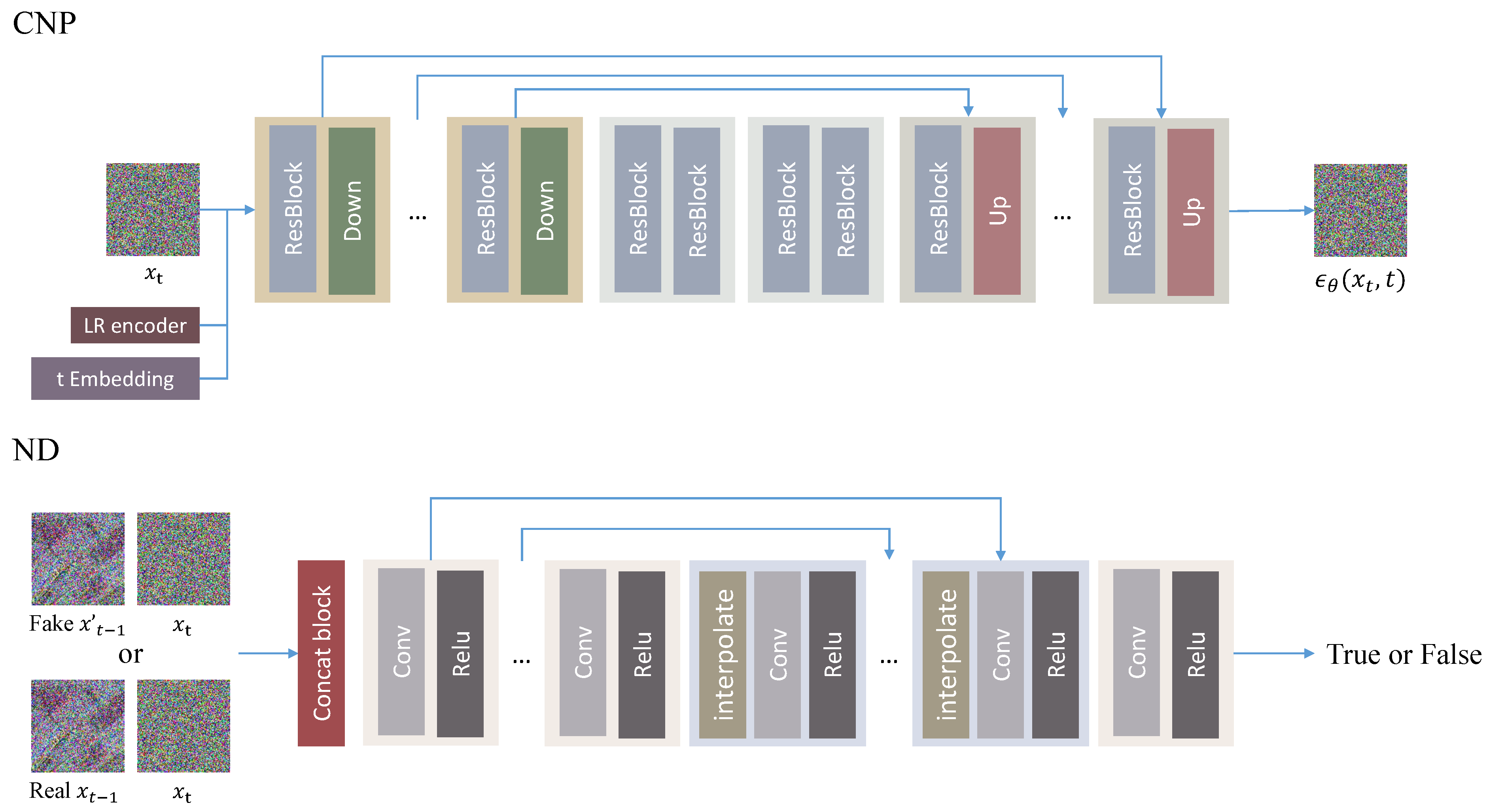
CNP produces the noise that needs to be eliminated from the noisy image, serving as the central component of the diffusion model. The process initiates with the input noise undergoing a convolution head, incorporating a convolution layer and Mish activation to augment channel numbers. Subsequently, it enters the core U-Net of the CNP, where it undergoes processing alongside the output of a pre-trained feature extraction model and diffusion timesteps . The diffusion timesteps are transformed using a positional encoding into a timestep embedding and guide the generated noise strength of the CNP. As depicted in Figure 2, the CNP comprises three segments: the contracting step, the middle step, and the expansive step. In the contracting step, four blocks focus on enhancing channels, each containing two residual blocks and a downsampling layer. LR features are fused with the hidden state output by the first two residual blocks in the initial block of the contracting step. Conversely, the expansive steps consist of blocks containing two residual blocks and an upsampling layer to reduce the channel number. To optimize the model size, the channel size only doubles in the second and fourth blocks, while the spatial size of the feature maps is halved in each block. Additionally, the middle step between them comprises only two residual blocks. Furthermore, the output of each block in the contracting step is added to the corresponding output of the expansive steps. After traversing the U-Net, a convolution tail is applied to generate the final predicted noise.
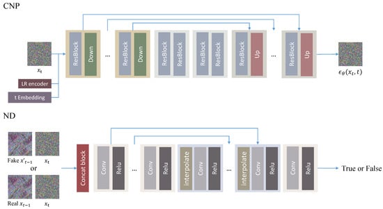
Figure 2.
The architecture of the CNP and ND. Up and Down represent upsampling and downsampling, respectively.
2.3. Noise Discriminator (ND)
To distinguish between the real and the generated , we introduce a Noise Discriminator (ND) designed to learn the overall correspondence between and . The architecture, depicted in Figure 2, follows the structure of [36]. The pair of and are initially concatenated along the channel axis and processed through a convolution operation. Convolutional groups incorporating Relu activation functions and convolutional layers are applied to down-sample the features. Following the down-sampling, an interpolation operation is introduced before the convolutional group to facilitate up-sampling. This up-sampling involves a skip connection that adds features with the same channels generated during both the down-sampling and up-sampling processes, promoting effective feature reuse. Finally, two convolutional groups are employed to integrate the features and generate the probability of whether in this pair is true.
2.4. Hybrid Loss Function for CNP
To enhance the capabilities of DiffALS, we introduce an extra adversarial loss function to facilitate the convergence of the CNP. Consequently, the loss function of DiffALS can be partitioned into two distinct components.
where is the loss function of the diffusion model mentioned in Equation (9), is our proposed adversarial loss of the ND and w is the weight hyper-parameter to balance the two loss functions.
2.4.1. Adversarial Loss
In conventional diffusion models, the CNP learns the data distribution by minimizing the disparity between actual noise and predicted noise during training. The supplementary adversarial loss prompts our CNP to prioritize solutions aligned with the manifold of real pairs and by attempting to fool the ND. ND discerns the relationship between adjacent noisy images, which encompass diverse information related to the image contents. Compared to conventional loss functions based on predicted noise, the adversarial loss enhances the detailed texture generation capability of the diffusion model by providing guidance based on image contents present in the training set. The loss value is determined by the probabilities generated by the ND across all samples and is defined as follows:
where refers to the discriminator and the output of , denoted as , represents the probability that the discriminator categorizes the pair (a, b) as real. If the ND can easily distinguish the fake pair with a low score of , it will incur a substantial loss function, thereby impacting the training of the CNP.
2.4.2. Loss for ND
The ND undergoes training with the CNP, fostering mutual improvement during the training process. The objective of the ND’s loss function is to enhance its ability to discriminate between genuine pairs of and and fake pairs and . If the ND assigns a high score to fake pairs or a low score to real pairs, the loss function imposes a significant penalty. The formal expression for the loss function pertaining to the ND is as follows:
2.5. Training and Inference
As depicted in Figure 1, in the training process, we first randomly initialize the CNP. Afterward, the residual results computed between the upsampled LR images and HR images are fused with a random noise to and fed into the CNP with t and the LR features extracted by the LR encoder. The and t are sampled from the standard Gaussian distribution and the integer set . Finally, the CNP is optimized with the hybrid loss function Equation (11). The noise discriminator also updates during the training process.
In the inference process, the LR images and the number of diffusion steps T are input. Firstly, a random noise following the Gaussian distribution is fed into the reverse process as . In each timestep, is sampled and then fed into the CNP with the features extracted from the LR encoder. After the CNP, the predicted noise and go through the Equation (10) to generate if . Finally, the outputs of the final results are fused with the upsampled LR images to get the SR images.
3. Results and Analysis
3.1. Datasets and Metrics
Our model underwent training and testing using three satellite RS datasets, namely, OLI2MSI [37], Alsat [38], and Vaihingen [39]. OLI2MSI comprises 5225 pairs of Landsat8-OLI (30 m) and Sentinel2-MSI (10 m) images as LR and HR images for training and 100 pairs for testing. In the Alsat dataset, the training set consists of 2182 pairs of LR (10 m) and HR (2.5 m) images. The test set is divided into three parts, including agriculture, urban, and special, with a total of 577 pairs. For the SR datasets, we aim to produce the HR image based on its corresponding LR image. Vaihingen is a segmentation dataset comprising 33 images with a ground sampling distance of 9 cm, which is utilized to assess the SR model’s performance in real-image applications. The segmentation labels encompass six classes: roads, buildings, cars, low vegetation, trees, and clutter. The effectiveness of our model in SR tasks is demonstrated through the utilization of OLI2MSI and Alsat datasets. Additionally, the Vaihingen dataset serves as a platform to showcase the effectiveness of our model in downstream applications such as segmentation. Detailed implementation of our model on the Vaihingen dataset is elaborated in Section 3.4. For model evaluation, we employ various metrics, including Peak Signal-to-Noise Ratio (PSNR) [9], Structural Similarity (SSIM) [9], Fréchet Inception Distance (FID) [40], and Learned Perceptual Image Patch Similarity (LPIPS) [41], to assess the quality of the restored images. PSNR emphasizes pixel-level differences between two images, while SSIM calculates structural similarity. LPIPS evaluates images in a manner that approximates human judgment. Lower LPIPS values signify greater similarity, whereas higher values indicate greater dissimilarity. FID, designed for evaluating generative models, measures the Fréchet distance between two distributions in the activation space of a pre-trained image classification model to assess the similarity between image sets. Additionally, visual comparisons are presented to illustrate the significant improvements achieved by our method.
3.2. Implementation Details
Our experiments are conducted with the PyTorch framework and executed on a single NVIDIA GeForce RTX 4090 GPU with 24G RAM. The number of channels is set to and in CNP and ND, respectively, while the kernel size for CNP and the up-sampling process in ND are both fixed at 3. The LR encoder adopts the architecture of RRDB [36]. Furthermore, the weight of the adversarial loss w is designated as 0.5. Throughout the training and testing of the diffusion model, the number of diffusion steps for each image is configured to be 100. The noise schedules, denoted as , adhere to the settings employed in SRDiff [33].
Our network is trained using loss in the CNP and loss in the ND, employing a batch size of 16 and a learning rate of . For the two SR datasets, LR and HR image pairs are randomly extracted as 32 × 32 patches and 96 × 96 patches in OLI2MSI, and 32 × 32 patches and 128 × 128 patches in Alsat, with a scaling factor of 3 or 4 during the training step. In testing, the images are centrally cropped to match the size of the training data. As for the segmentation dataset, since each image in the Vaihingen dataset is a size of about 2000 × 2500, we divide each image into HR images of a size of 128 × 128 and bicubically resized to LR images of 32 × 32. In total, 8478 images are utilized in training, while 2187 images are employed in testing. Each model is trained and tested on each dataset separately.
3.3. Performance
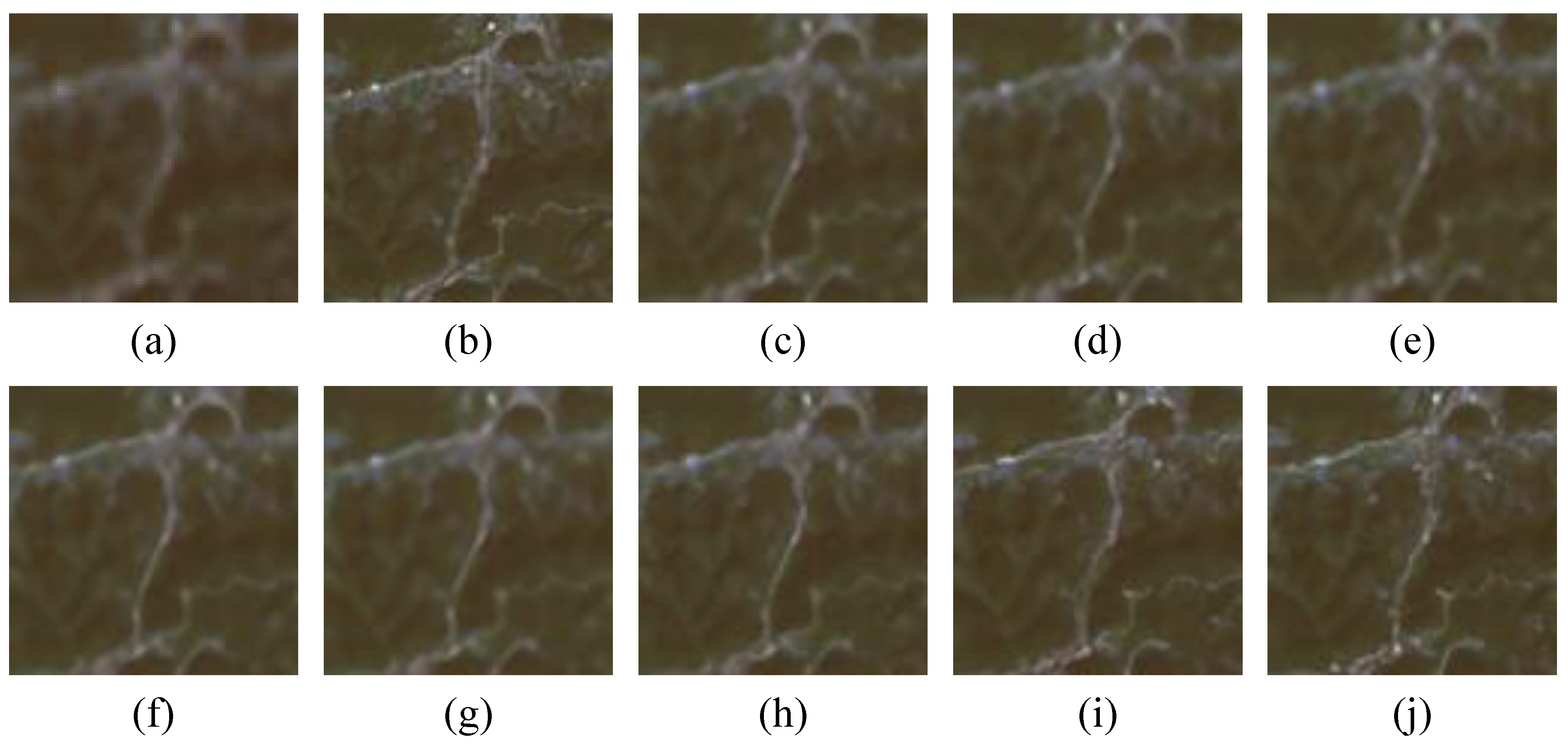
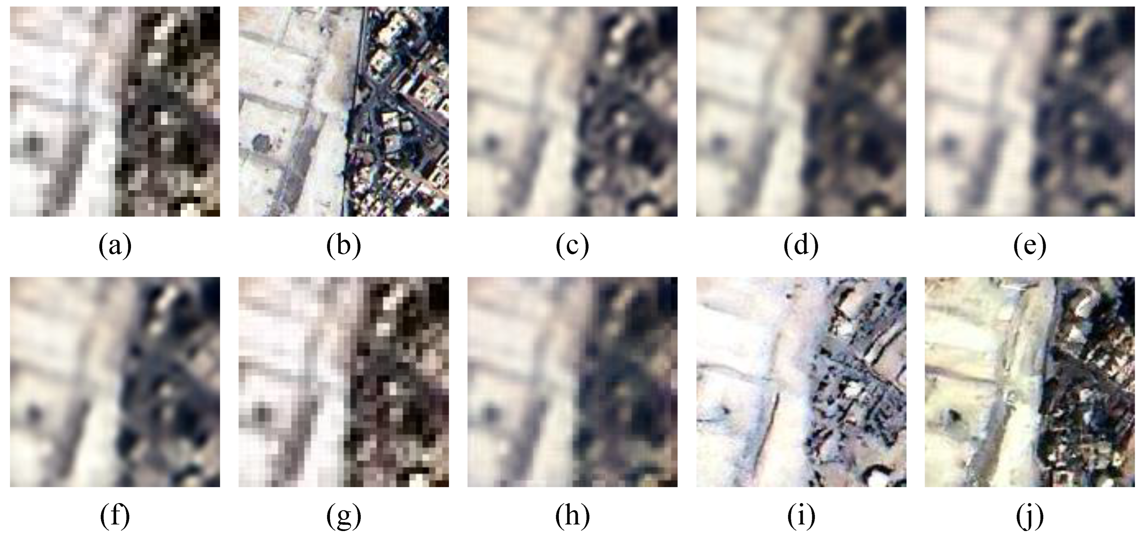
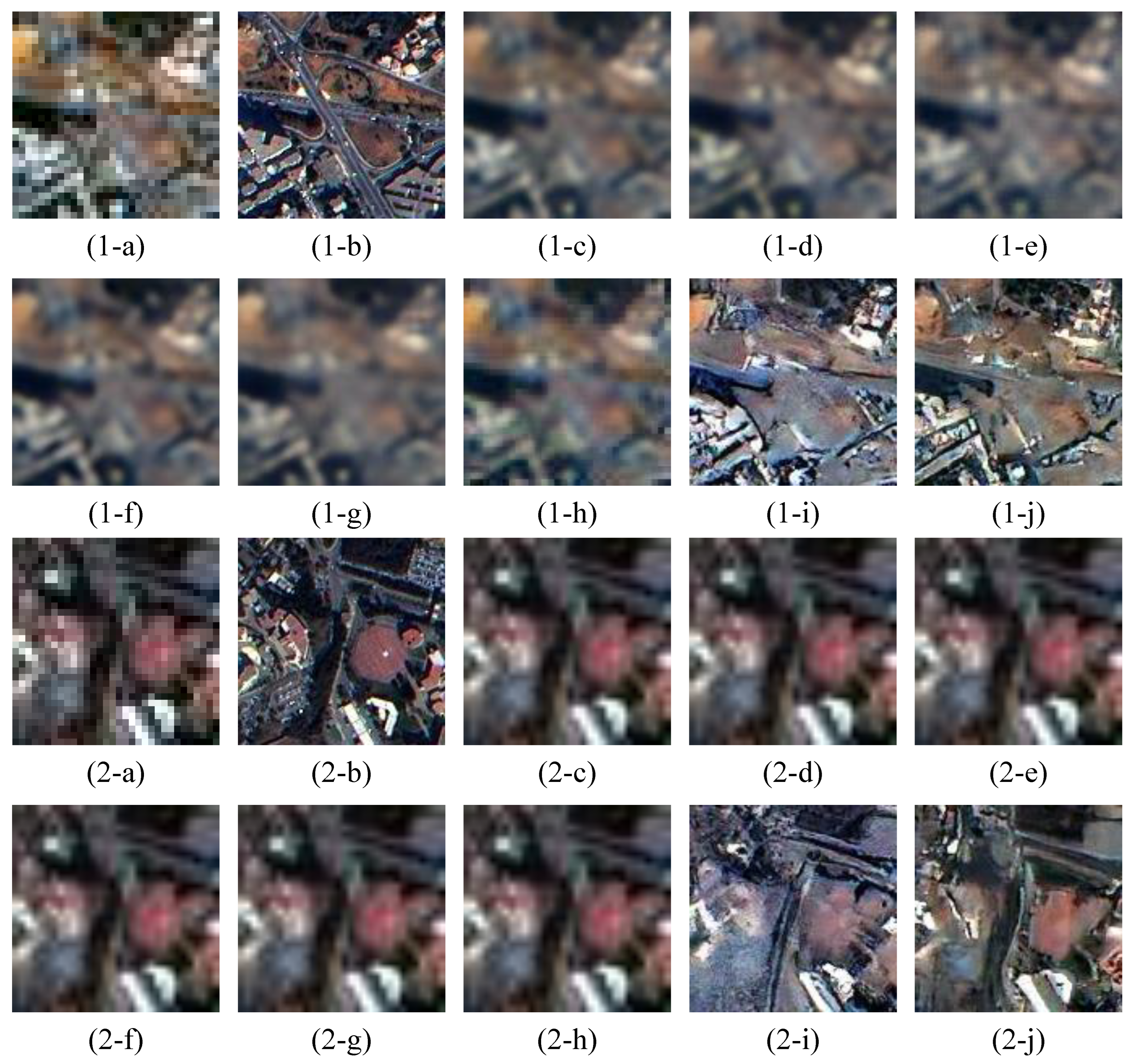
In order to validate our proposed model, we compare it with seven different types of state-of-the-art models, including four CNN-based models EFDN [42], DBPN [43], ESRT [27], NLSN [44], three generative models SRGAN [45], ESRGAN [36] and our baseline SRDiff [33]. The experimental results on OLI2MSI and Alsat are shown in Table 1 and Table 2, respectively. The visual comparisons of the SISR are presented in Figure 3 and Figure 4. Additional visual results are available in Appendix A.

Table 1.
The quantitative experimental results on the OLI2MSI. The best is bolded. ↑ and ↓ represent higher better and lower better, respectively.

Table 2.
The quantitative experimental results on the Alsat. The best is bolded. ↑ and ↓ represent higher better and lower better, respectively.
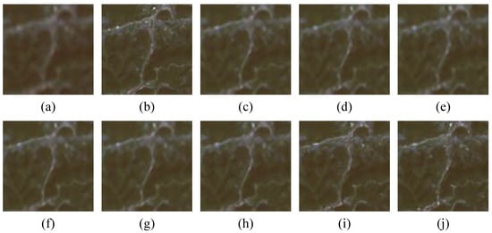
Figure 3.
The visual comparisons on the OLI2MSI. (a) LR. (b) HR. (c) EFDN. (d) DBPN. (e) ESRT. (f) NLSN. (g) SRGAN. (h) ESRGAN. (i) SRDiff. (j) DiffALS.
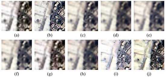
Figure 4.
The visual comparisons on the Alsat. (a) LR. (b) HR. (c) EFDN. (d) DBPN. (e) ESRT. (f) NLSN. (g) SRGAN. (h) ESRGAN. (i) SRDiff. (j) DiffALS.
Our model demonstrates substantial improvement in perceptual quality, as indicated by FID and LPIPS gains of 23 and 0.002 in the OLI2MSI dataset, and 189 and 0.002 in the Alsat dataset, compared to our baseline SRDiff. Regarding PSNR and SSIM, DiffALS achieves results comparable to SRDiff, indicating that the introduction of the ND enhances perceptual quality without compromising accuracy. This notable enhancement positions DiffALS as a viable solution for high-scale SISR tasks, showcasing considerable developmental potential. Diffusion-based models outperform previous methods in terms of visual evaluation metrics, highlighting their effectiveness in generating superior SR images based on human judgment. Nevertheless, they exhibit lower PSNR and SSIM compared to GAN-based and CNN-based models, indicating lower accuracy at the pixel level. To substantiate that the images generated by our DiffALS indeed achieve superior accuracy and perceptual quality, rather than merely inducing human perception, we conduct additional experiments applying the SR images to broader applications. The forthcoming section will showcase that our model indeed yields superior SR images that are more suitable for downstream applications.
Concerning perceptual quality, SR images restored by conventional CNN-based models exhibit over-smoothing and blurriness due to their reliance solely on corresponding LR images for generation. This lack of detailed LR information limits the performance of CNN-based models, particularly in high-scale SISR tasks. EFDN, DBPN, ESRT, and NLSN show minimal improvement in terms of clarity compared to LR images. The perceptual quality of SR images produced by GAN-based models appears superior to that of CNN-based models. However, GAN-based models commonly encounter challenges such as model collapse, unstable training, and vanishing gradients, negatively impacting their representation. Notably, GAN-based models still primarily rely on pixel-level content loss, explaining why SRGAN and ESRGAN exhibit slight improvement compared to CNN-based models.
Comparing SRDiff and DiffALS results, both of them generate SR images that outperform GAN-based and CNN-based models in terms of sharpness and detail. Nevertheless, our model excels over SRDiff in providing more detailed and reliable texture information. For instance, in visual comparisons of Figure 4, the texture on the left side of the SR image generated by DiffALS is richer than SRDiff. Moreover, on the right side of the SR image, SRDiff fails to generate the outline of the building accurately.
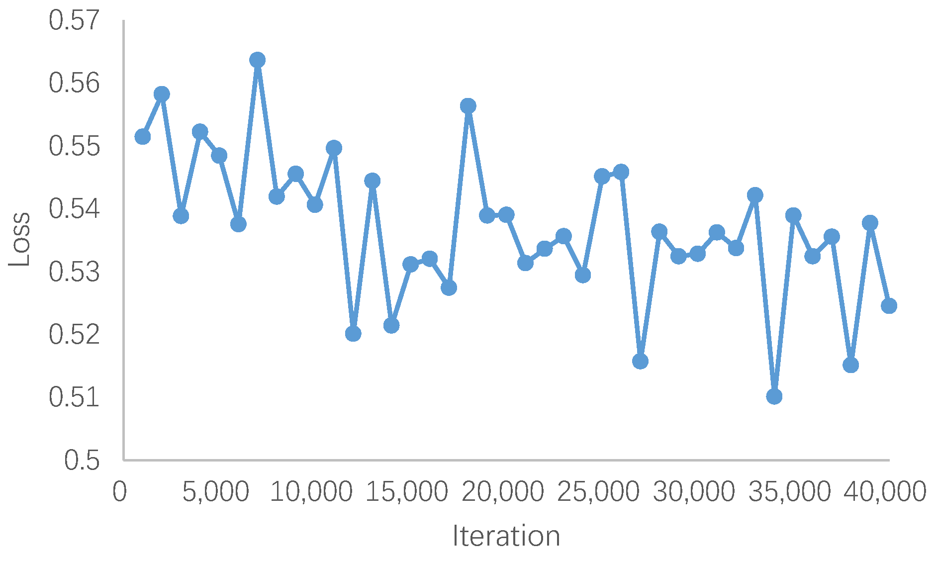
The iteration curve for our DiffALS model on OLI2MSI is depicted in Figure 5. Since the noise added to images in the training process is randomly sampled from the Gaussian distribution, the loss function exhibits significant fluctuations. The training process of the diffusion model exhibits considerable instability. Ultimately, we train the model for 40,000 epochs to achieve optimal results.
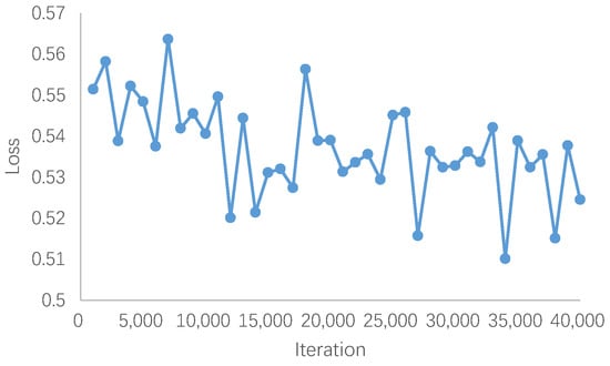
Figure 5.
The iteration curve of our DiffALS on OLI2MSI.
3.4. Extension Experiment
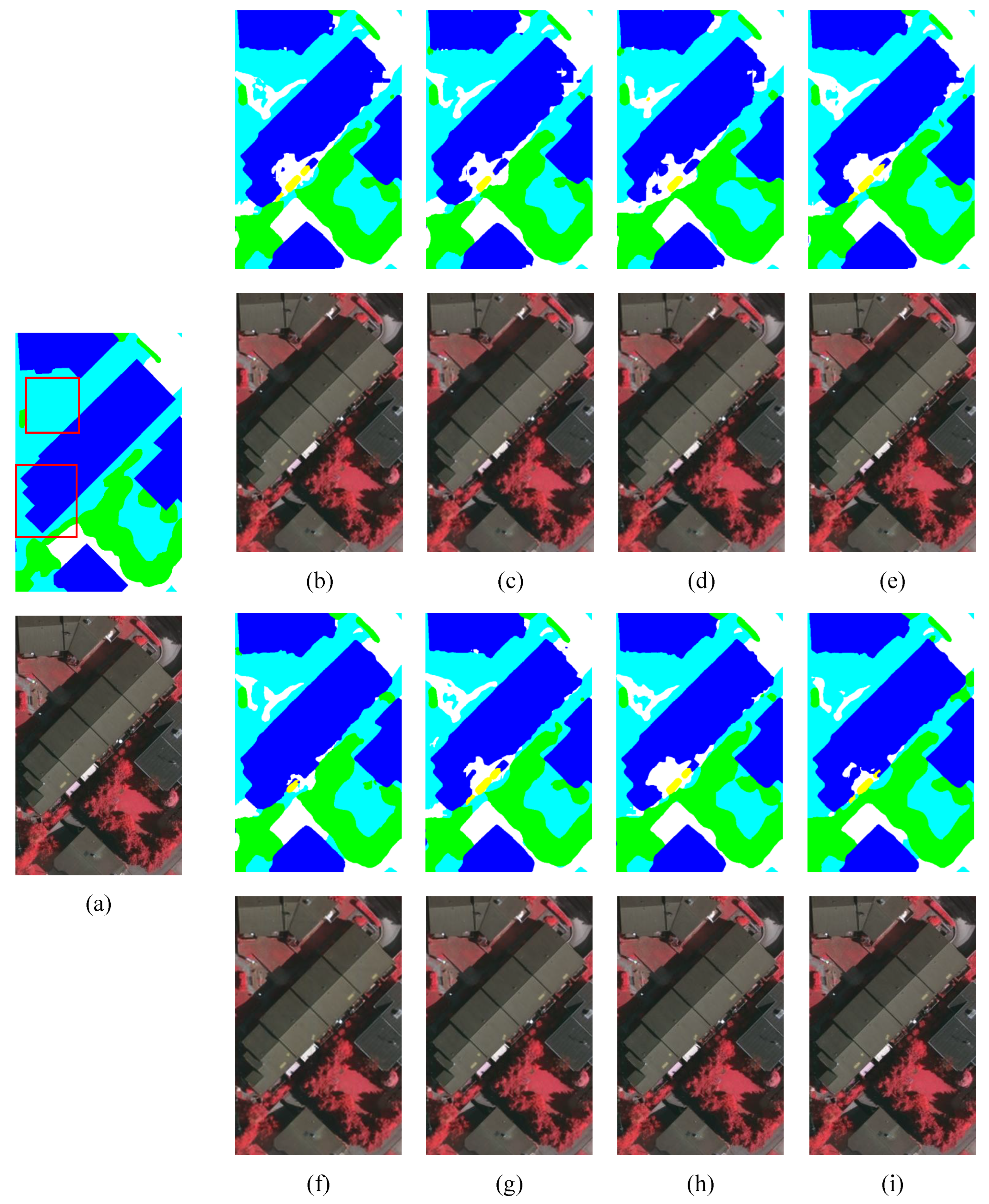
To further validate the efficacy of our proposed DiffALS, we conduct additional experiments on a segmentation dataset called Vaihingen. Initially, we partition and resize the images using bicubic interpolation to of their original size, resulting in ground sampling distances of 9 cm for HR images and 36 cm for LR images. Subsequently, we utilize a variety of SISR models to produce the corresponding SR images. We compare these SR images with the HR images and evaluate the segmentation results using a pre-trained Unetformer [46]. The SISR and segmentation outcomes are presented in Table 3, Table 4 and Table 5, while visualizations are depicted in Figure 6.

Table 3.
The quantitative experimental results on the Vaihingen. The best is bolded. ↑ and ↓ represent higher better and lower better, respectively.

Table 4.
The quantitative experimental results on the Vaihingen. The best is bolded.

Table 5.
The quantitative experimental results for five main classes on the Vaihingen. The best is bolded.

Figure 6.
The visual comparisons on the Vaihingen. The main difference between those models is circled with red boxes. (a) HR. (b) EFDN. (c) DBPN. (d) ESRT. (e) NLSN. (f) SRGAN. (g) ESRGAN. (h) SRDiff. (i) DiffALS.
As shown in Table 3, our DiffALS also demonstrates superior results in terms of human perception, with improvements of approximately 53 and 0.006 in FID and LPIPS, respectively, compared to our baseline SRDiff. Despite the fact that CNN-based and GAN-based models exhibit higher PSNR and SSIM values than diffusion-based models, SRDiff and DiffALS outperform them in visual effects and segmentation tasks. As shown in Table 4, SRDiff achieves an increase of approximately 0.5% in F1 score, 1.4% in MIoU, and 1.3% in Accuracy compared to the best result among GAN-based models, ESRGAN. Additionally, SRDiff outperforms the best CNN-based model, NLSN, with an increase of approximately 1.1% in F1 score, 1.5% in MIoU, and 1.5% in Accuracy. In comparison to our baseline SRDiff, DiffALS significantly surpasses it by margins of 0.4%, 0.3%, and 0.2% in F1 score, MIoU, and Accuracy, respectively. These results underscore the effectiveness of our model in real-world applications.
We also provide comprehensive IoU values for each class, excluding clutter in our experiments. As indicated in Table 5, our DiffALS consistently achieves the best results, maintaining advantages in per-class IoU. Specifically, DiffALS outperforms SRDiff by 0.7%, 0.4%, 0.3%, 0.2%, and 0.2% in the roads, buildings, low vegetation, trees, and cars. The richly detailed textures generated by our models appear to enhance the segmentation network’s ability to distinguish between different object types. Notably, our diffusion-based models outperform CNN-based and GAN-based models across almost all classes.
3.5. Parameter Analysis
To assess the impact of the ND, we perform experiments with different weights w for the adversarial loss in , on the OLI2MSI dataset as depicted in Table 6. We note that the image quality exhibits low sensitivity to the weight of the adversarial loss from 0.1 to 0.7. Notably, all weights surpass the performance of our baseline model, SRDiff, in terms of FID and LPIPS. These findings underscore the stability and efficacy of our model.

Table 6.
The quantitative experimental results on the Vaihingen. ↑ and ↓ represent higher better and lower better, respectively.
3.6. Running Time Comparison
In Table 7, we present a comparison of the computational cost across all methods, considering model complexity, memory usage, parameters, and inference speed. Model complexity is assessed in Giga Floating-point Operations Per Second (GFLOPs), where . Memory usage is measured in megabytes (MB), while the number of parameters is denoted in millions (M). Finally, the inference speed is indicated in frames per second (FPS). The complexity, memory usage, and speed collectively reflect the efficiency of the models in the inference process. All the experiments are implemented on a single NVIDIA GeForce RTX 4090 GPU with 24G RAM.

Table 7.
Running time comparison of all methods.
The models in our study are categorized into three groups: CNN-based, GAN-based, and diffusion-based models. If a model utilizes a discriminator during training, such as SRGAN, ESRGAN, and DiffALS, the parameters of the discriminator are included in the total model parameters. It is notable that the complexity, memory usage, and speed of our proposed DiffALS are similar to SRDiff since their inference processes are identical. The adversarial learning strategy of our DiffALS is exclusively effective during the training phase. The results in Table 7 reveal that diffusion-based models demonstrate higher computational complexity, resulting in notably slower inference speeds compared to other models. The complexity, memory usage, and parameters are comparable to that of other models.
4. Discussion
It is worth noting that although diffusion-based models exhibit lower PSNR and SSIM scores compared to CNN-based and GAN-based models, they excel in segmentation results. This observation supports that our model genuinely produces high-quality SR images that not only perform better under human perception but also genuinely benefit the downstream application. Consequently, the improved performance in both visual results and downstream applications serves as evidence of the effectiveness of our model. These results still underscore the limitations of relying on PSNR and SSIM as metrics for evaluating model performance in SR applications.
5. Conclusions
In this study, we present a diffusion model incorporating an adversarial learning strategy for achieving clear and detailed SR image reconstruction, particularly tailored for RS applications. The DiffALS model incorporates ND into the data distribution learning of the diffusion model, providing supplementary guidance in the noise prediction process by taking into account the inherent correlation between adjacent noisy images. The adversarial loss derived from ND enhances both the detailed texture generation capability and the diversity of generated data in the diffusion model, utilizing image contents from the entire training set. Furthermore, a distinctive metric derived from real-world semantic segmentation outcomes has been utilized to illustrate that our SR images exhibit superior performance in human perception and downstream applications. These results still highlight the limitations of the conventional metrics, such as PSNR and SSIM, which previous researchers have predominantly focused on. Experiments on three satellite RS datasets, namely Alsat, OLO2MSI, and Vaihingen, validate the effectiveness and generalizability of our proposed DiffALS model. Though it exhibits slower inference speeds, the complexity, memory usage, and parameter counts of our DiffALS align with the state-of-the-art models.
Acknowledging the need for further research, particularly in optimizing the balance between diffusion and adversarial losses, we anticipate improvements in the overall performance of the model. And it is still worth further investigation on the performance of the diffusion model endowed with other noise distributions besides the Gaussian noise commonly used in the diffusion model [15]. Moreover, it is of great practical importance to establish new strategies to expedite the training process of the diffusion model. For example, LR images can be processed into various forms to facilitate the convergence of the diffusion model.
Author Contributions
Conceptualization, J.S. and Q.W.; methodology, J.S.; software, J.S.; validation, J.S. and M.-O.P.; formal analysis, J.S. and M.-O.P.; writing—original draft preparation, J.S., Q.W. and M.-O.P.; writing—review and editing, J.S., Q.W. and M.-O.P.; supervision, M.-O.P.; All authors have read and agreed to the published version of the manuscript.
Funding
This work was supported in part by the National Key R&D Program of China under Grant 2018YFB1800800, in part by the Basic Research Project under Grant HZQB-KCZYZ-2021067 of Hetao Shenzhen-HK S&T Cooperation Zone, Shenzhen Outstanding Talents Training Fund under Grant 202002, in part by Guangdong Research Projects under Grant 2017ZT07X152 and Grant 2019CX01X104, in part by the Guangdong Provincial Key Laboratory of Future Networks of Intelligence under Grant 2022B1212010001, in part by the National Natural Science Foundation of China under Grant 41801323, and in part by the National Key Research and Development Program of China under Grant 2020YFA0714003.
Data Availability Statement
The datasets are available online at https://github.com/achrafdjerida/Alsat-2B and https://github.com/wjwjww/OLI2MSI (accessed on 30 December 2023).
Conflicts of Interest
The authors declare no conflicts of interest.
Abbreviations
The following abbreviations are used in this manuscript:
| SISR | Single-Image Super-Resolution |
| RS | Remote Sensing |
| DL | Deep Learning |
| CNN | Convolutional Neural Network |
| GAN | Generative Adversarial Network |
| LR | Low-Resolution |
| HR | High-Resolution |
| SR | Super-Resolution |
| DiffALS | Diffusion model with Adversarial Learning Strategy |
| ND | Noise Discriminator |
| CNP | Conditional Noise Predictor |
| PSNR | Peak Signal-to-Noise Ratio |
| SSIM | Structural Similarity Index |
| FID | Fréchet Inception Distance |
| LPIPS | Learned Perceptual Image Patch Similarity |
Appendix A
Appendix A.1
Additional examples of the visual comparisons on the OLI2MSI and Alsat.
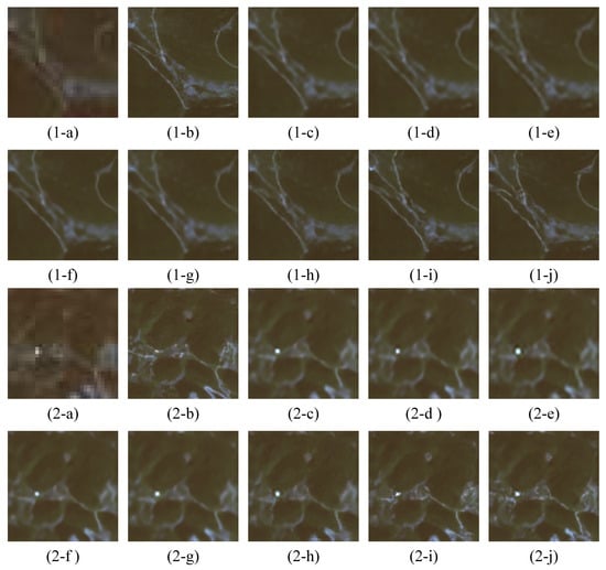
Figure A1.
The visual comparisons on the OLI2MSI dataset. (a) LR. (b) HR. (c) EFDN. (d) DBPN. (e) ESRT. (f) NLSN. (g) SRGAN. (h) ESRGAN. (i) SRDiff. (j) DiffALS.
Figure A1.
The visual comparisons on the OLI2MSI dataset. (a) LR. (b) HR. (c) EFDN. (d) DBPN. (e) ESRT. (f) NLSN. (g) SRGAN. (h) ESRGAN. (i) SRDiff. (j) DiffALS.
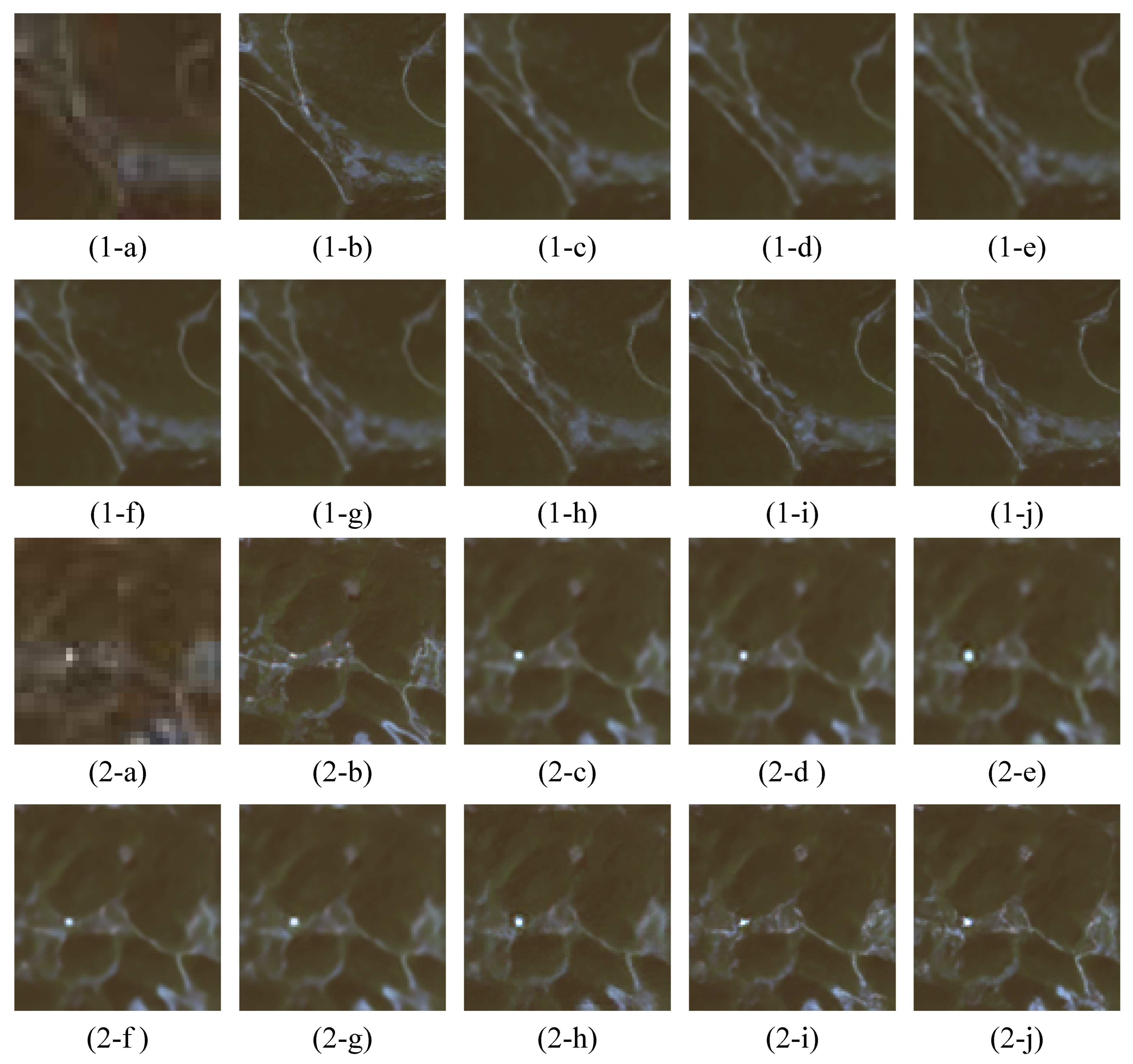
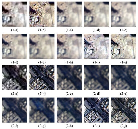
Figure A2.
The visual comparisons on the Alsat “special" set. (a) LR. (b) HR. (c) EFDN. (d) DBPN. (e) ESRT. (f) NLSN. (g) SRGAN. (h) ESRGAN. (i) SRDiff. (j) DiffALS.
Figure A2.
The visual comparisons on the Alsat “special" set. (a) LR. (b) HR. (c) EFDN. (d) DBPN. (e) ESRT. (f) NLSN. (g) SRGAN. (h) ESRGAN. (i) SRDiff. (j) DiffALS.
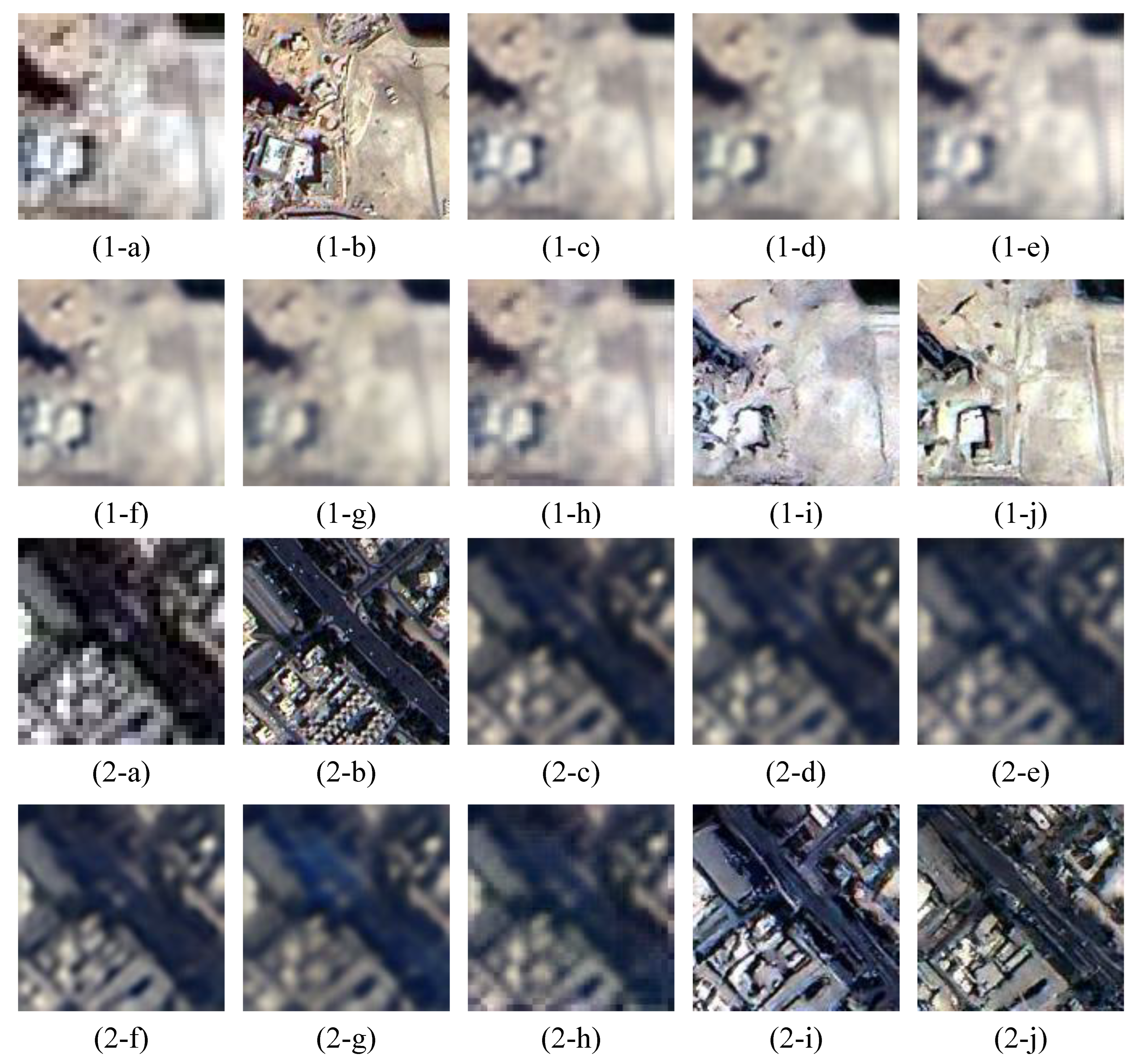
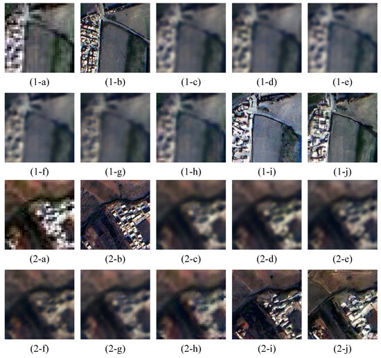
Figure A3.
The visual comparisons on the Alsat “agriculture” set. (a) LR. (b) HR. (c) EFDN. (d) DBPN. (e) ESRT. (f) NLSN. (g) SRGAN. (h) ESRGAN. (i) SRDiff. (j) DiffALS.
Figure A3.
The visual comparisons on the Alsat “agriculture” set. (a) LR. (b) HR. (c) EFDN. (d) DBPN. (e) ESRT. (f) NLSN. (g) SRGAN. (h) ESRGAN. (i) SRDiff. (j) DiffALS.
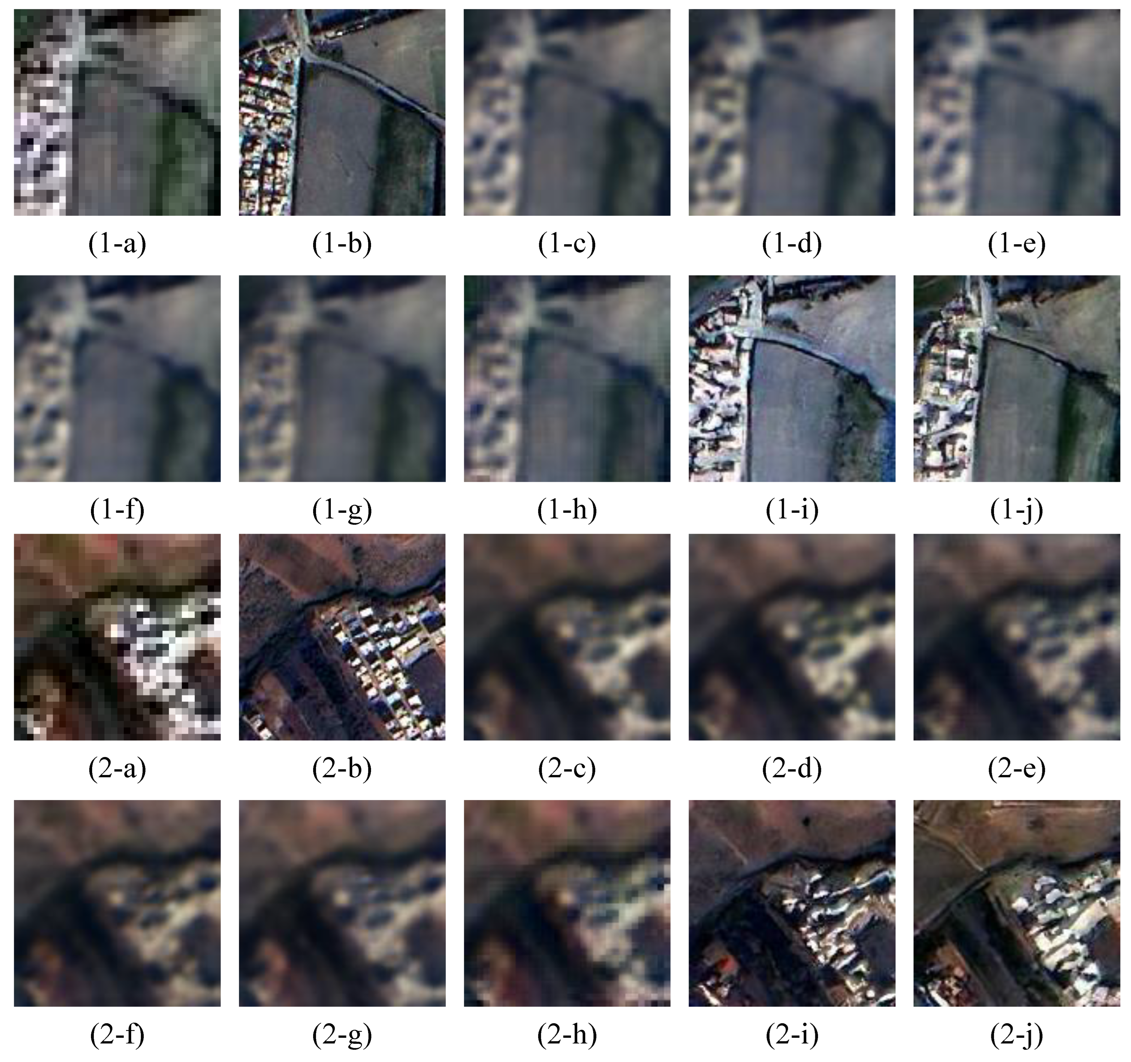

Figure A4.
The visual comparisons on the Alsat “urban” set. (a) LR. (b) HR. (c) EFDN. (d) DBPN. (e) ESRT. (f) NLSN. (g) SRGAN. (h) ESRGAN. (i) SRDiff. (j) DiffALS.
Figure A4.
The visual comparisons on the Alsat “urban” set. (a) LR. (b) HR. (c) EFDN. (d) DBPN. (e) ESRT. (f) NLSN. (g) SRGAN. (h) ESRGAN. (i) SRDiff. (j) DiffALS.
References
- Willis, K.S. Remote sensing change detection for ecological monitoring in United States protected areas. Biol. Conserv. 2015, 182, 233–242. [Google Scholar] [CrossRef]
- Zhang, X.; Yu, W.; Pun, M.O.; Shi, W. Cross-domain landslide mapping from large-scale remote sensing images using prototype-guided domain-aware progressive representation learning. ISPRS J. Photogramm. Remote. Sens. 2023, 197, 1–17. [Google Scholar] [CrossRef]
- Zhang, X.; Yu, W.; Pun, M.O. Multilevel deformable attention-aggregated networks for change detection in bitemporal remote sensing imagery. IEEE Trans. Geosci. Remote. Sens. 2022, 60, 5621518. [Google Scholar] [CrossRef]
- Lin, J.; Gao, F.; Shi, X.; Dong, J.; Du, Q. SS-MAE: Spatial–spectral masked autoencoder for multisource remote sensing image classification. IEEE Trans. Geosci. Remote. Sens. 2023, 61, 1–14. [Google Scholar] [CrossRef]
- Xiao, T.; Liu, Y.; Huang, Y.; Li, M.; Yang, G. Enhancing multiscale representations with transformer for remote sensing image semantic segmentation. IEEE Trans. Geosci. Remote. Sens. 2023, 61, 1–16. [Google Scholar] [CrossRef]
- Ma, X.; Wu, Q.; Zhao, X.; Zhang, X.; Pun, M.O.; Huang, B. SAM-Assisted Remote Sensing Imagery Semantic Segmentation with Object and Boundary Constraints. arXiv 2023, arXiv:2312.02464. [Google Scholar]
- Lepcha, D.C.; Goyal, B.; Dogra, A.; Goyal, V. Image super-resolution: A comprehensive review, recent trends, challenges and applications. Inf. Fusion 2023, 91, 230–260. [Google Scholar] [CrossRef]
- Chen, H.; He, X.; Qing, L.; Wu, Y.; Ren, C.; Sheriff, R.E.; Zhu, C. Real-world single image super-resolution: A brief review. Inf. Fusion 2022, 79, 124–145. [Google Scholar] [CrossRef]
- Wang, P.; Bayram, B.; Sertel, E. A comprehensive review on deep learning based remote sensing image super-resolution methods. Earth-Sci. Rev. 2022, 232, 104110. [Google Scholar] [CrossRef]
- Wang, Y.; Bashir, S.M.A.; Khan, M.; Ullah, Q.; Wang, R.; Song, Y.; Guo, Z.; Niu, Y. Remote sensing image super-resolution and object detection: Benchmark and state of the art. Expert Syst. Appl. 2022, 197, 116793. [Google Scholar] [CrossRef]
- Mu, R.; Zeng, X. A review of deep learning research. KSII Trans. Internet Inf. Syst. 2019, 13, 1738–1764. [Google Scholar]
- Deng, L.; Yu, D. Deep learning: Methods and applications. Found. Trends® Signal Process. 2014, 7, 197–387. [Google Scholar] [CrossRef]
- Li, H.; Jia, C.; Jin, P.; Cheng, Z.; Li, K.; Sui, J.; Liu, C.; Yuan, L. FreestyleRet: Retrieving Images from Style-Diversified Queries. arXiv 2023, arXiv:2312.02428. [Google Scholar]
- Wang, K.; Gou, C.; Duan, Y.; Lin, Y.; Zheng, X.; Wang, F.Y. Generative adversarial networks: Introduction and outlook. IEEE/CAA J. Autom. Sin. 2017, 4, 588–598. [Google Scholar] [CrossRef]
- Ho, J.; Jain, A.; Abbeel, P. Denoising Diffusion Probabilistic Models. In Advances in Neural Information Processing Systems; Larochelle, H., Ranzato, M., Hadsell, R., Balcan, M., Lin, H., Eds.; Curran Associates, Inc.: Red Hook, NY, USA, 2020; Volume 33, pp. 6840–6851. [Google Scholar]
- Sui, J.; Ma, X.; Zhang, X.; Pun, M.O. GCRDN: Global Context-Driven Residual Dense Network for Remote Sensing Image Super-Resolution. IEEE J. Sel. Top. Appl. Earth Obs. Remote. Sens. 2023, 16, 4457–4468. [Google Scholar] [CrossRef]
- Sui, J.; Ma, X.; Zhang, X.; Pun, M.O. DTRN: Dual Transformer Residual Network for Remote Sensing Super-Resolution. In Proceedings of the IGARSS 2023-2023 IEEE International Geoscience and Remote Sensing Symposium, Pasadena, CA, USA, 16–21 July 2023; IEEE: New York, NY, USA, 2023; pp. 6041–6044. [Google Scholar]
- Dong, X.; Sun, X.; Jia, X.; Xi, Z.; Gao, L.; Zhang, B. Remote sensing image super-resolution using novel dense-sampling networks. IEEE Trans. Geosci. Remote. Sens. 2020, 59, 1618–1633. [Google Scholar] [CrossRef]
- Pan, Z.; Ma, W.; Guo, J.; Lei, B. Super-resolution of single remote sensing image based on residual dense backprojection networks. IEEE Trans. Geosci. Remote. Sens. 2019, 57, 7918–7933. [Google Scholar] [CrossRef]
- Wang, S.; Zhou, T.; Lu, Y.; Di, H. Contextual transformation network for lightweight remote-sensing image super-resolution. IEEE Trans. Geosci. Remote. Sens. 2021, 60, 5615313. [Google Scholar] [CrossRef]
- Kim, J.; Lee, J.K.; Lee, K.M. Accurate image super-resolution using very deep convolutional networks. In Proceedings of the IEEE Conference on Computer Vision and Pattern Recognition, Las Vegas, NV, USA, 27–30 June 2016; pp. 1646–1654. [Google Scholar]
- Tai, Y.; Yang, J.; Liu, X. Image super-resolution via deep recursive residual network. In Proceedings of the IEEE Conference on Computer Vision and Pattern Recognition, Honolulu, HI, USA, 21–26 July 2017; pp. 3147–3155. [Google Scholar]
- Zhang, Y.; Tian, Y.; Kong, Y.; Zhong, B.; Fu, Y. Residual dense network for image super-resolution. In Proceedings of the IEEE Conference on Computer Vision and Pattern Recognition, Salt Lake City, UT, USA, 18–23 June 2018; pp. 2472–2481. [Google Scholar]
- Yang, Y.; Zhang, D.; Huang, S.; Wu, J. Multilevel and multiscale network for single-image super-resolution. IEEE Signal Process. Lett. 2019, 26, 1877–1881. [Google Scholar] [CrossRef]
- Chen, Z.; Tian, S.; Shi, X.; Lu, H. Multiscale shared learning for fault diagnosis of rotating machinery in transportation infrastructures. IEEE Trans. Ind. Inform. 2022, 19, 447–458. [Google Scholar] [CrossRef]
- Feng, J.; Jiang, Q.; Tseng, C.H.; Jin, X.; Liu, L.; Zhou, W.; Yao, S. A deep multitask convolutional neural network for remote sensing image super-resolution and colorization. IEEE Trans. Geosci. Remote. Sens. 2022, 60, 1–15. [Google Scholar] [CrossRef]
- Lu, Z.; Li, J.; Liu, H.; Huang, C.; Zhang, L.; Zeng, T. Transformer for single image super-resolution. In Proceedings of the IEEE/CVF Conference on Computer Vision and Pattern Recognition, New Orleans, LA, USA, 18–24 June 2022; pp. 457–466. [Google Scholar]
- Liu, Y.; Hu, J.; Kang, X.; Luo, J.; Fan, S. Interactformer: Interactive transformer and CNN for hyperspectral image super-resolution. IEEE Trans. Geosci. Remote. Sens. 2022, 60, 5531715. [Google Scholar] [CrossRef]
- Jia, S.; Wang, Z.; Li, Q.; Jia, X.; Xu, M. Multiattention generative adversarial network for remote sensing image super-resolution. IEEE Trans. Geosci. Remote. Sens. 2022, 60, 5624715. [Google Scholar] [CrossRef]
- Dong, R.; Zhang, L.; Fu, H. RRSGAN: Reference-based super-resolution for remote sensing image. IEEE Trans. Geosci. Remote. Sens. 2021, 60, 5601117. [Google Scholar] [CrossRef]
- Creswell, A.; White, T.; Dumoulin, V.; Arulkumaran, K.; Sengupta, B.; Bharath, A.A. Generative adversarial networks: An overview. IEEE Signal Process. Mag. 2018, 35, 53–65. [Google Scholar] [CrossRef]
- Saharia, C.; Ho, J.; Chan, W.; Salimans, T.; Fleet, D.J.; Norouzi, M. Image super-resolution via iterative refinement. IEEE Trans. Pattern Anal. Mach. Intell. 2022, 45, 4713–4726. [Google Scholar] [CrossRef] [PubMed]
- Li, H.; Yang, Y.; Chang, M.; Chen, S.; Feng, H.; Xu, Z.; Li, Q.; Chen, Y. Srdiff: Single image super-resolution with diffusion probabilistic models. Neurocomputing 2022, 479, 47–59. [Google Scholar] [CrossRef]
- Xiao, Y.; Yuan, Q.; Jiang, K.; He, J.; Jin, X.; Zhang, L. EDiffSR: An efficient diffusion probabilistic model for remote sensing image super-resolution. IEEE Trans. Geosci. Remote. Sens. 2023, 62, 5601514. [Google Scholar] [CrossRef]
- Han, L.; Zhao, Y.; Lv, H.; Zhang, Y.; Liu, H.; Bi, G.; Han, Q. Enhancing remote sensing image super-resolution with efficient hybrid conditional diffusion model. Remote. Sens. 2023, 15, 3452. [Google Scholar] [CrossRef]
- Wang, X.; Yu, K.; Wu, S.; Gu, J.; Liu, Y.; Dong, C.; Qiao, Y.; Change Loy, C. Esrgan: Enhanced super-resolution generative adversarial networks. In Proceedings of the European Conference on Computer Vision (ECCV) Workshops, Munich, Germany, 8–14 September 2018. [Google Scholar]
- Wang, J.; Gao, K.; Zhang, Z.; Ni, C.; Hu, Z.; Chen, D.; Wu, Q. Multisensor Remote Sensing Imagery Super-Resolution with Conditional GAN. J. Remote. Sens. 2021, 2021, 9829706. [Google Scholar] [CrossRef]
- Djerida, A.; Djerriri, K.; Karoui, M.S. A new public Alsat-2B dataset for single-image super-resolution. In Proceedings of the 2021 IEEE International Geoscience and Remote Sensing Symposium IGARSS, Brussels, Belgium, 11–16 July 2021; IEEE: New York, NY, USA, 2021; pp. 8095–8098. [Google Scholar]
- Gerke, M. Use of the Stair Vision Library within the ISPRS 2D Semantic Labeling Benchmark (Vaihingen). 2014. Available online: https://www.researchgate.net/publication/270104226_Use_of_the_Stair_Vision_Library_within_the_ISPRS_2D_Semantic_Labeling_Benchmark_Vaihingen?channel=doi&linkId=54ae59c50cf2828b29fcdf4b&showFulltext=true (accessed on 22 March 2024).
- Heusel, M.; Ramsauer, H.; Unterthiner, T.; Nessler, B.; Hochreiter, S. Gans trained by a two time-scale update rule converge to a local nash equilibrium. Adv. Neural Inf. Process. Syst. 2017, 6627–6638. [Google Scholar]
- Zhang, R.; Isola, P.; Efros, A.A.; Shechtman, E.; Wang, O. The unreasonable effectiveness of deep features as a perceptual metric. In Proceedings of the IEEE Conference on Computer Vision and Pattern Recognition, Salt Lake City, UT, USA, 18–23 June 2018; pp. 586–595. [Google Scholar]
- Wang, Y. Edge-enhanced feature distillation network for efficient super-resolution. In Proceedings of the IEEE/CVF Conference on Computer Vision and Pattern Recognition, New Orleans, LA, USA, 18–24 June 2022; pp. 777–785. [Google Scholar]
- Haris, M.; Shakhnarovich, G.; Ukita, N. Deep back-projection networks for super-resolution. In Proceedings of the IEEE Conference on Computer Vision and Pattern Recognition, Salt Lake City, UT, USA, 18–23 June 2018; pp. 1664–1673. [Google Scholar]
- Mei, Y.; Fan, Y.; Zhou, Y. Image super-resolution with non-local sparse attention. In Proceedings of the IEEE/CVF Conference on Computer Vision and Pattern Recognition, Virtually, 19–25 June 2021; pp. 3517–3526. [Google Scholar]
- Ledig, C.; Theis, L.; Huszár, F.; Caballero, J.; Cunningham, A.; Acosta, A.; Aitken, A.; Tejani, A.; Totz, J.; Wang, Z.; et al. Photo-realistic single image super-resolution using a generative adversarial network. In Proceedings of the IEEE Conference on Computer Vision and Pattern Recognition, Honolulu, HI, USA, 21–26 July 2017; pp. 4681–4690. [Google Scholar]
- Wang, L.; Li, R.; Zhang, C.; Fang, S.; Duan, C.; Meng, X.; Atkinson, P.M. UNetFormer: A UNet-like transformer for efficient semantic segmentation of remote sensing urban scene imagery. ISPRS J. Photogramm. Remote. Sens. 2022, 190, 196–214. [Google Scholar] [CrossRef]
Disclaimer/Publisher’s Note: The statements, opinions and data contained in all publications are solely those of the individual author(s) and contributor(s) and not of MDPI and/or the editor(s). MDPI and/or the editor(s) disclaim responsibility for any injury to people or property resulting from any ideas, methods, instructions or products referred to in the content. |
© 2024 by the authors. Licensee MDPI, Basel, Switzerland. This article is an open access article distributed under the terms and conditions of the Creative Commons Attribution (CC BY) license (https://creativecommons.org/licenses/by/4.0/).


