

An Object-Based Approach to Extract Aquaculture Ponds with 10-Meter Resolution Sentinel-2 Images: A Case Study of Wenchang City in Hainan Province


Abstract
1. Introduction
2. Materials and Methods
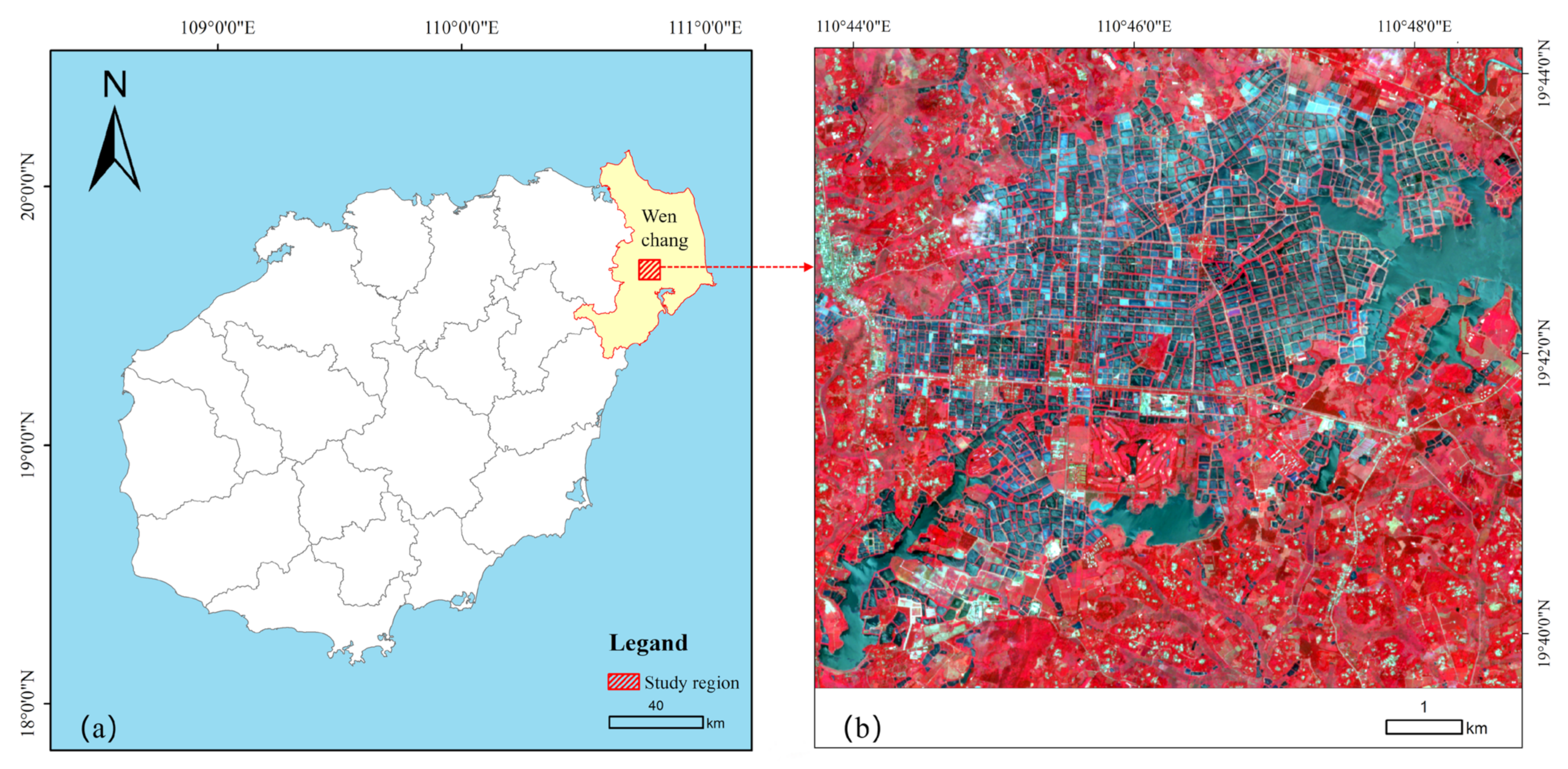
2.1. Study Area
2.2. Data
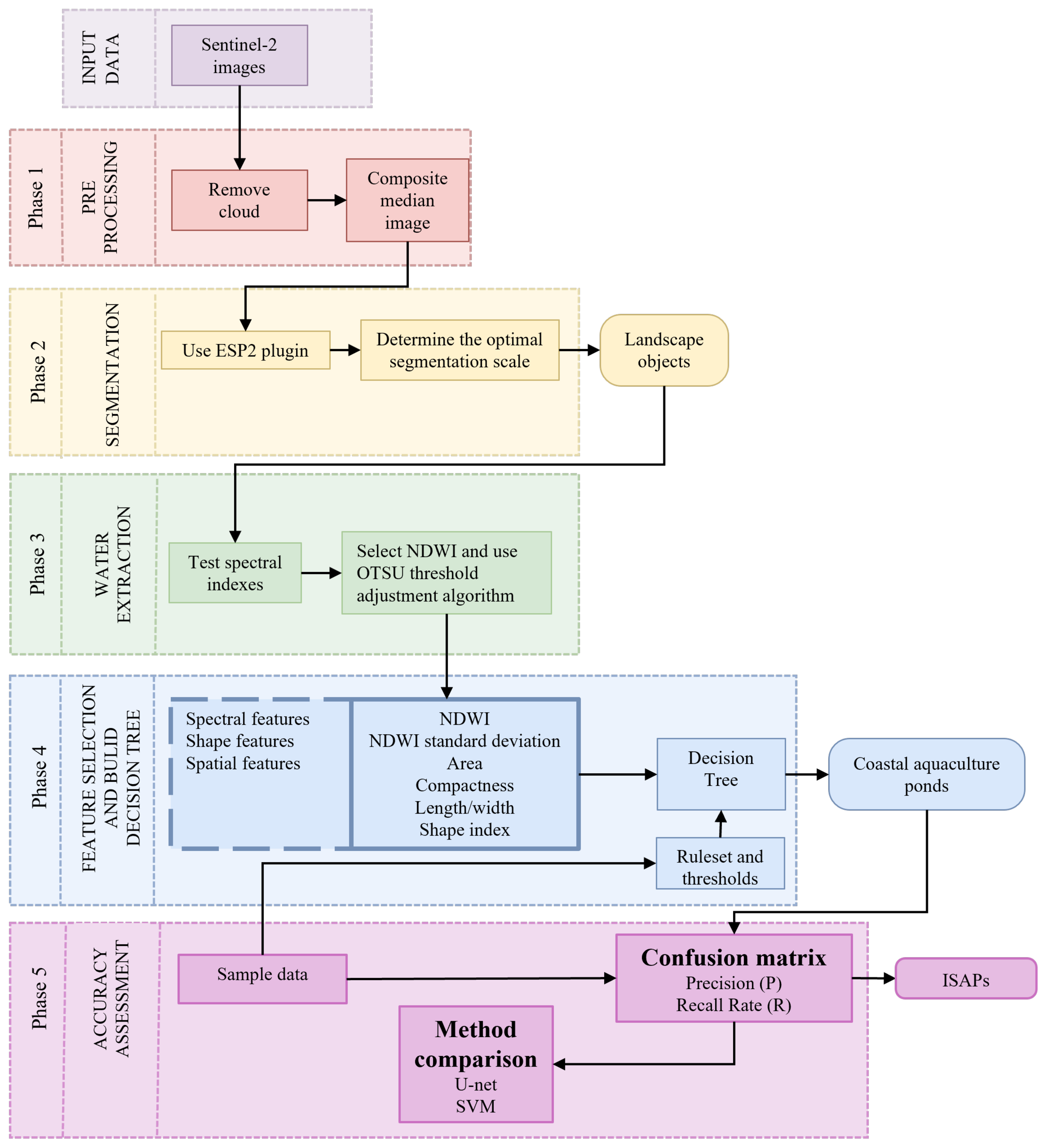
2.3. Method
2.3.1. Generating Objects via Segmentation
2.3.2. Water Body Extraction Using Water Indices
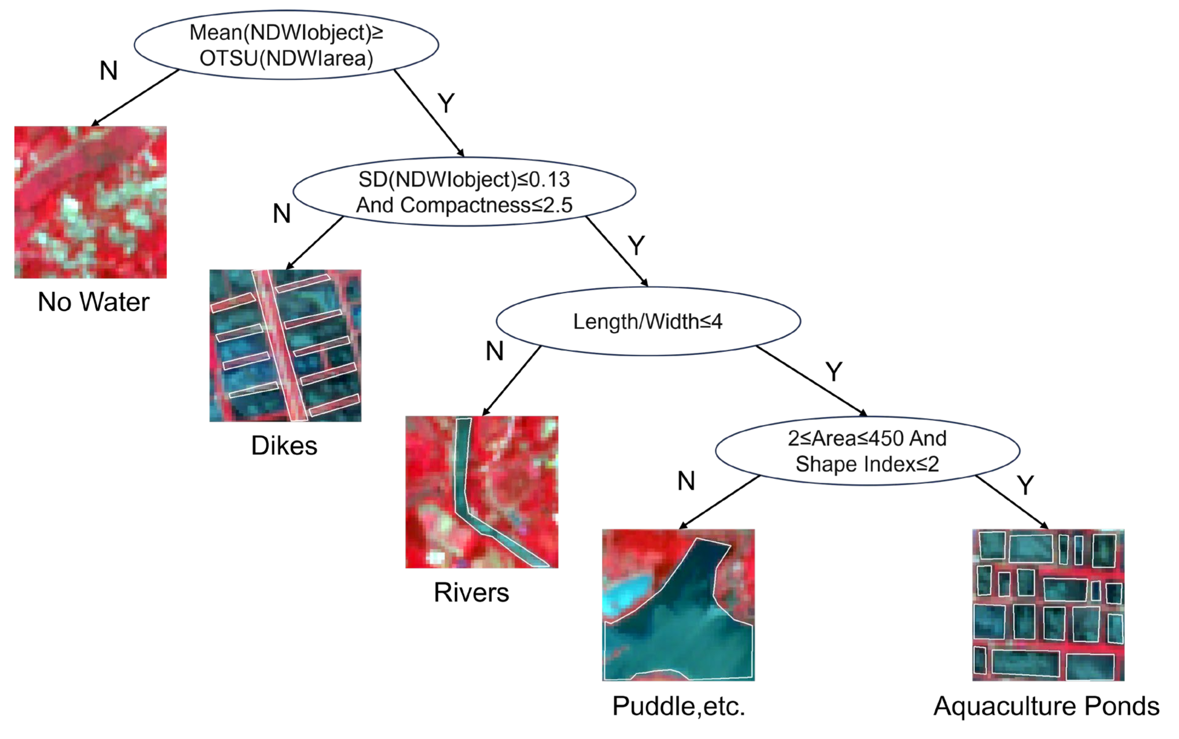
2.3.3. Establishing Classification Rule Sets
2.3.4. Extraction Method
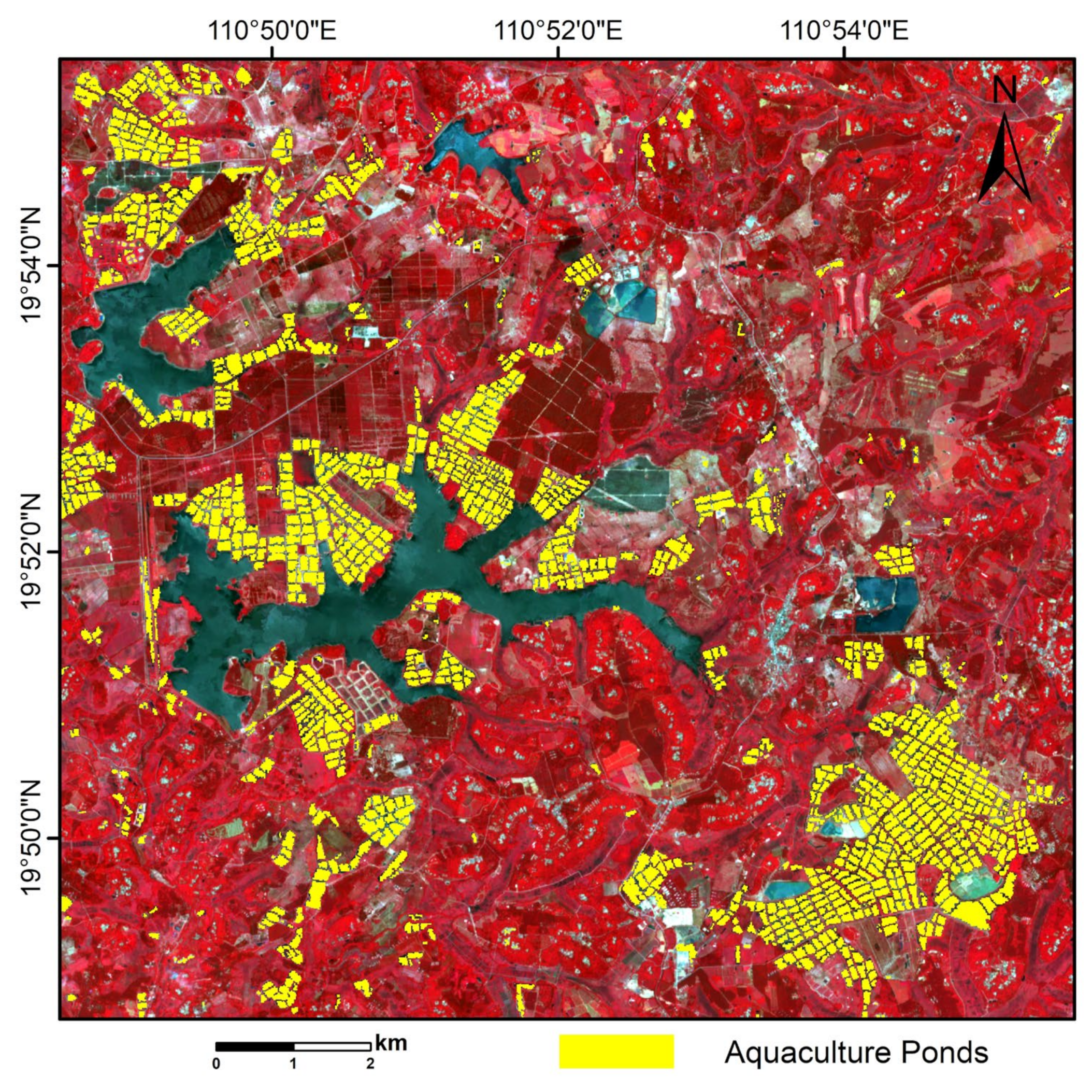
3. Results
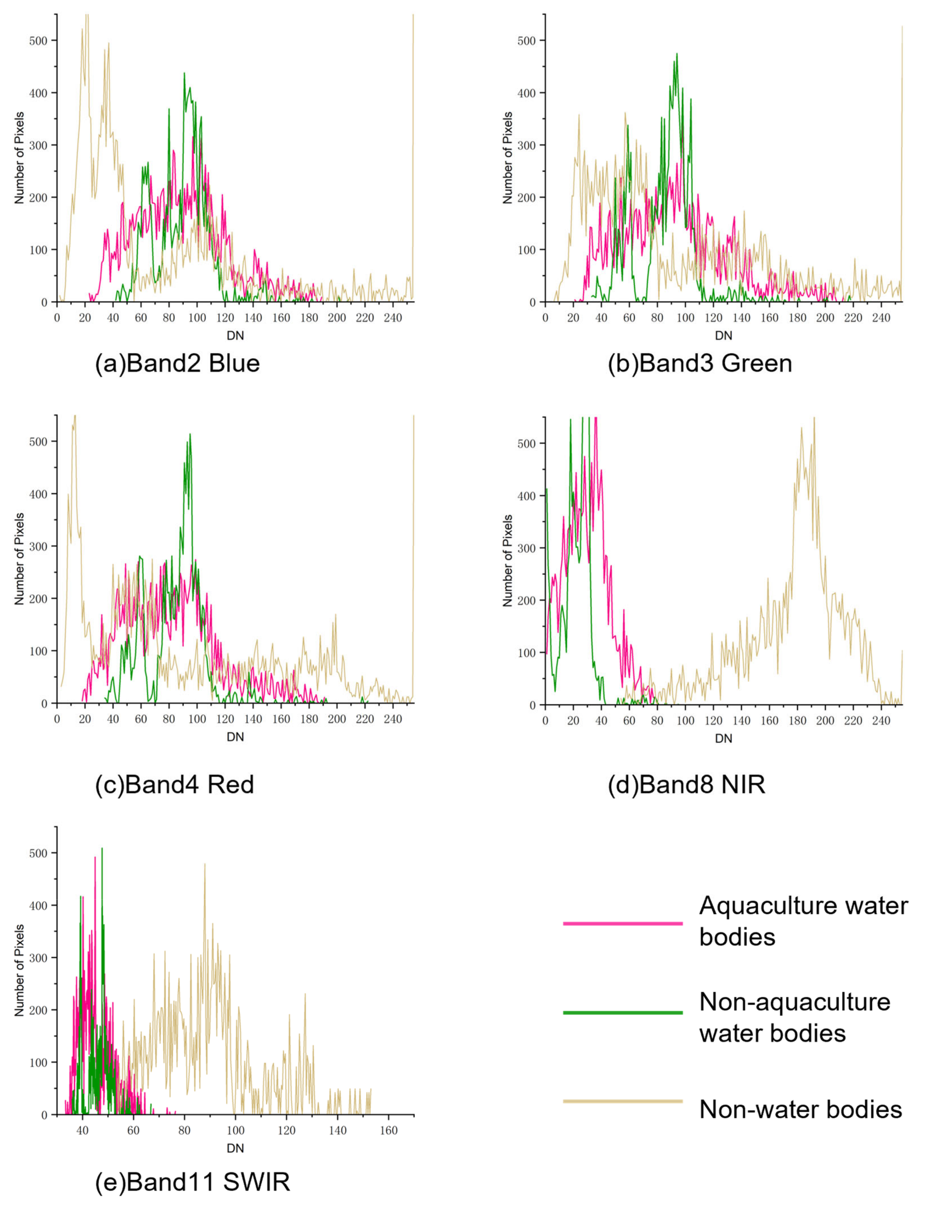
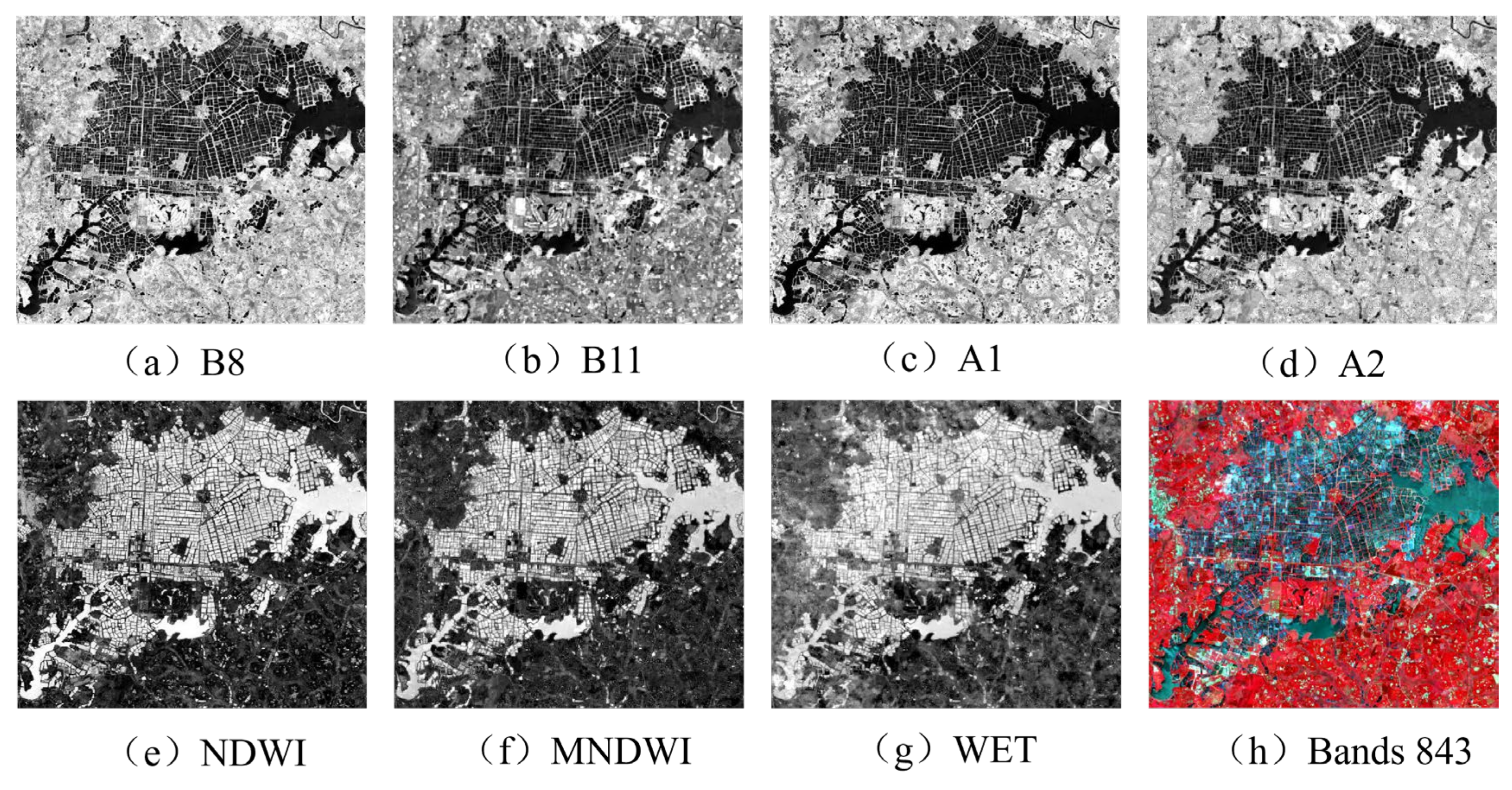
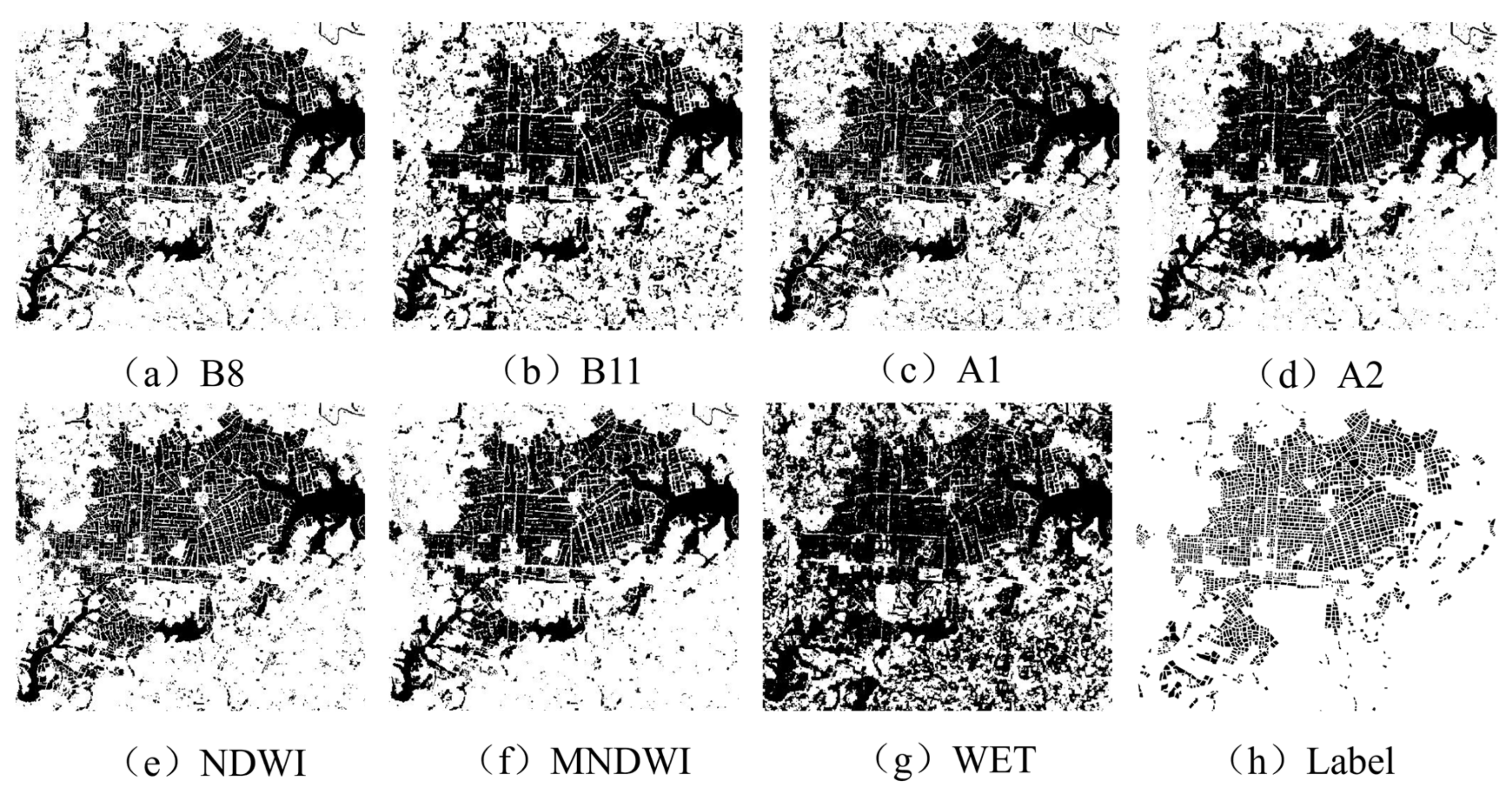
3.1. Water Body Extraction with Water Indices
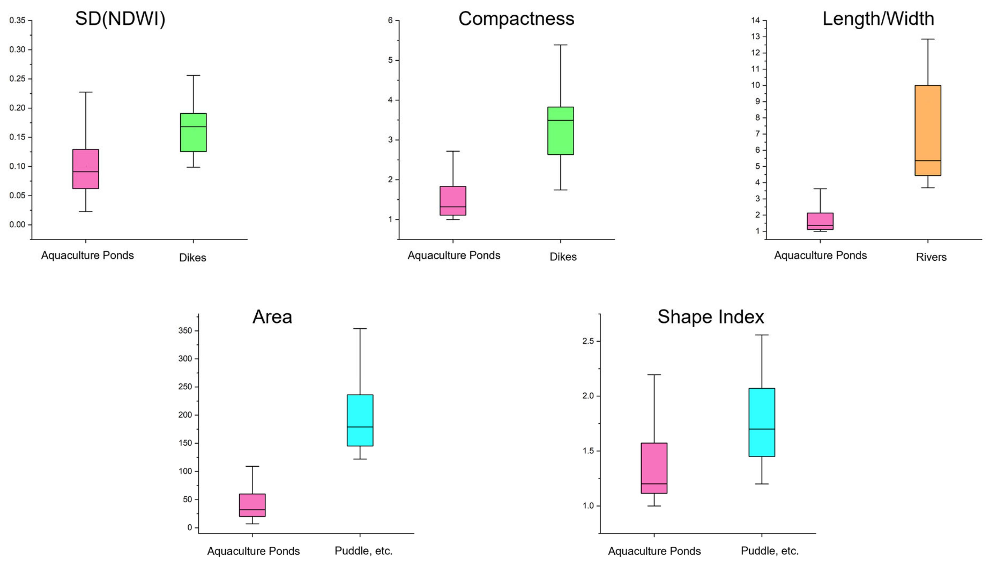
3.2. Feature Selection for Aquaculture Ponds
3.3. Extracting Coastal Aquaculture Pond Objects Using Decision Trees
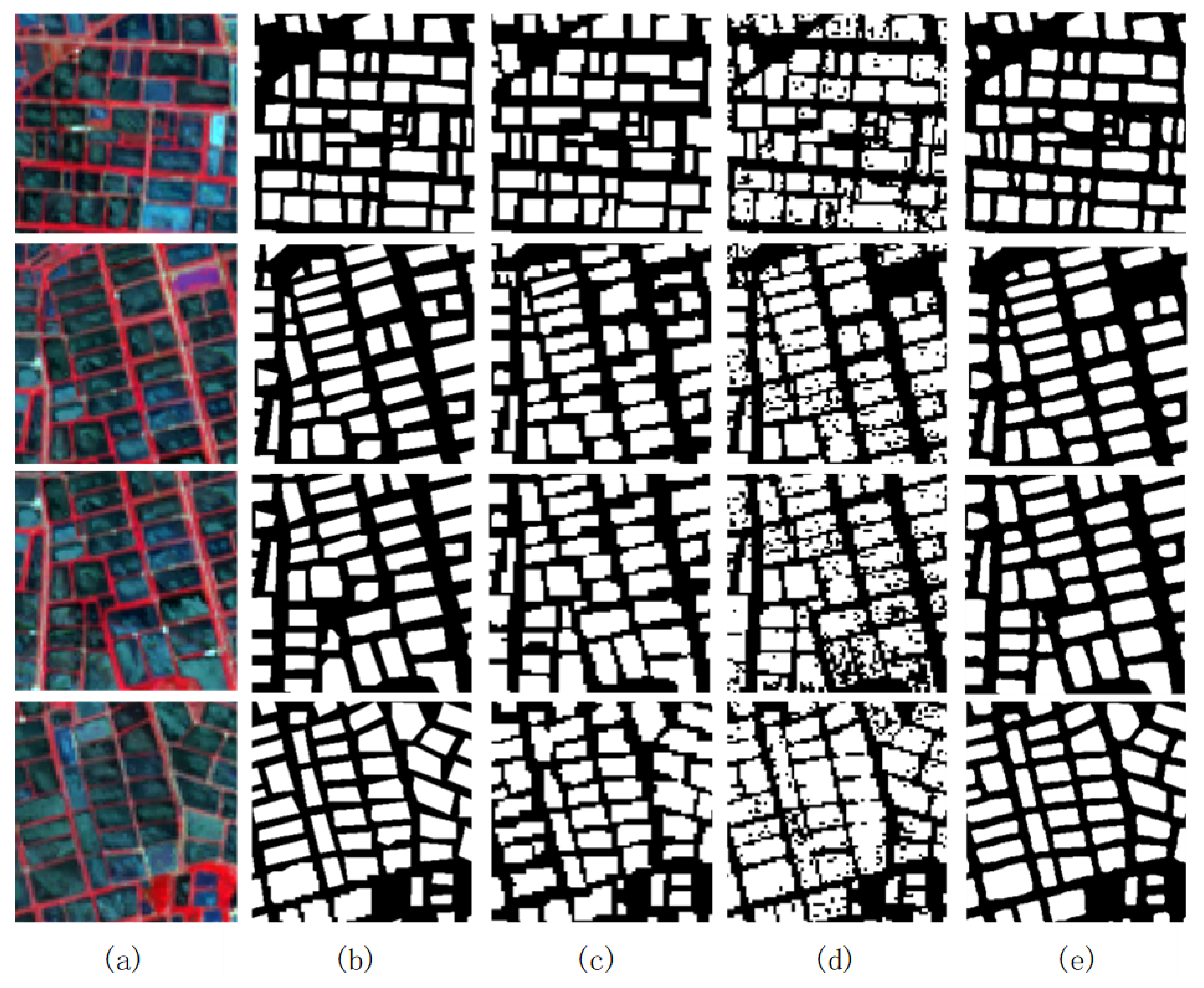
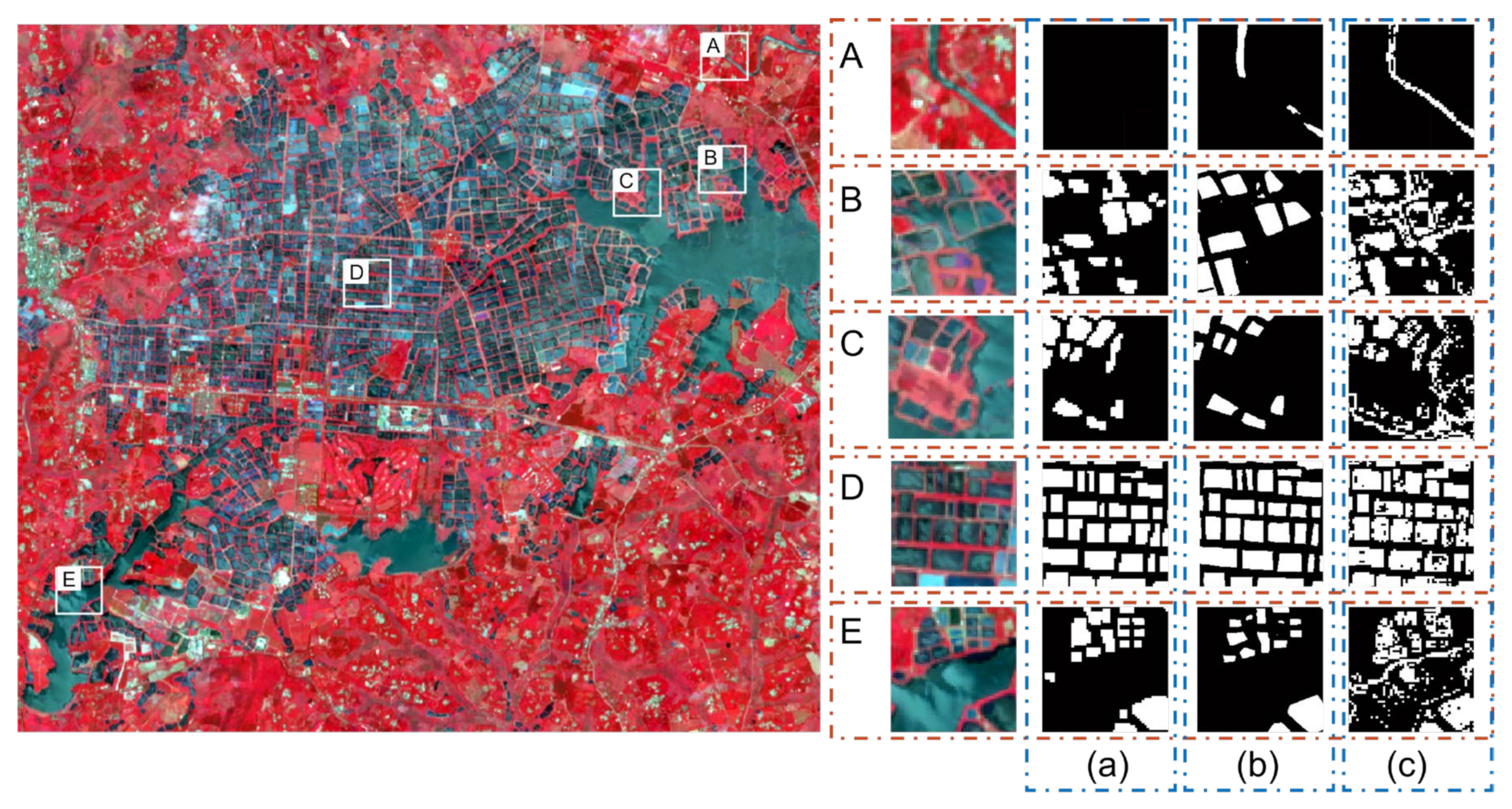
3.4. Accuracy Assessment
4. Discussion
4.1. The Analysis of the SVM Method
4.2. The Analysis of the Deep Learning Method
4.3. The Analysis of the Object-Based + Decision Tree Method
4.4. Potential for Transferability
5. Conclusions
- The proposed method can extract ISAPs with high accuracy; the accuracy (P) and recall (R) were around 85%, revealing that our method could effectively map aquaculture ponds.
- The proposed method showed better performance than SVM and U-Net. Our method can avoid adhesion and extract ISAPs that have previously not been accurately omitted from different water bodies. It is easy to operate and does not depend on the quality of local computer hardware, so it is suitable for the real-time and rapid extraction of large aquaculture areas.
- Our method has good transferability and can achieve an accuracy of more than 80% in the extraction of near-shore aquaculture ponds.
Author Contributions
Funding
Data Availability Statement
Acknowledgments
Conflicts of Interest
References
- Bank, M.S.; Metian, M.; Swarzenski, P.W. Defining Seafood Safety in the Anthropocene. Environ. Sci. Technol. 2020, 54, 8506–8508. [Google Scholar] [CrossRef] [PubMed]
- Jiang, Q.; Bhattarai, N.; Pahlow, M.; Xu, Z. Environmental Sustainability and Footprints of Global Aquaculture. Resour. Conserv. Recycl. 2022, 180, 106183. [Google Scholar] [CrossRef]
- Eswaran, H.; Lal, R.; Reich, P.F. Land degradation: An overview. In Response to Land Degradation; CRC Press: Boca Raton, FL, USA, 2019; pp. 20–35. [Google Scholar]
- Karami, F.; Shotorbani, P.M. Genetically modified foods: Pros and cons for human health. Food Health 2018, 1, 18–23. [Google Scholar]
- McFadden, B.R.; Lusk, J.L. What consumers don’t know about genetically modified food, and how that affects beliefs. FASEB J. 2016, 30, 3091–3096. [Google Scholar] [CrossRef]
- Yuan, J.; Xiang, J.; Liu, D.; Kang, H.; He, T.; Kim, S.; Lin, Y.; Freeman, C.; Ding, W. Rapid Growth in Greenhouse Gas Emissions from the Adoption of Industrial-Scale Aquaculture. Nat. Clim. Chang. 2019, 9, 318–322. [Google Scholar] [CrossRef]
- Minahal, Q.; Munir, S.; Komal, W.; Fatima, S.; Liaqat, R.; Shehzadi, I. Global impact of COVID-19 on aquaculture and fisheries: A review. Int. J. Fish. Aquat. Stud. 2020, 8, 42–48. [Google Scholar]
- Nasr-Allah, A.; Gasparatos, A.; Karanja, A.; Dompreh, E.B.; Murphy, S.; Rossignoli, C.M.; Phillips, M.; Charo-Karisa, H. Employment Generation in the Egyptian Aquaculture Value Chain: Implications for Meeting the Sustainable Development Goals (SDGs). Aquaculture 2020, 520, 734940. [Google Scholar] [CrossRef]
- Food and Agriculture Organization (FAO). The State of World Fisheries and Aquaculture 2022. Towards Blue Transformation; FAO: Rome, Italy, 2022; ISBN 978-92-5-136364-5. [Google Scholar]
- Wu, X.; Fu, B.; Wang, S.; Song, S.; Li, Y.; Xu, Z.; Wei, Y.; Liu, J. Decoupling of SDGs Followed by Re-Coupling as Sustainable Development Progresses. Nat. Sustain. 2022, 5, 452–459. [Google Scholar] [CrossRef]
- Subasinghe, R.; Soto, D.; Jia, J. Global Aquaculture and Its Role in Sustainable Development. Rev. Aquac. 2009, 1, 2–9. [Google Scholar] [CrossRef]
- Ren, C.; Wang, Z.; Zhang, Y.; Zhang, B.; Chen, L.; Xi, Y.; Xiao, X.; Doughty, R.B.; Liu, M.; Jia, M.; et al. Rapid expansion of coastal aquaculture ponds in China from Landsat observations during 1984–2016. Int. J. Appl. Earth Obs. Geoinf. 2019, 82, 101902. [Google Scholar] [CrossRef]
- Liu, D.; Keesing, J.K.; Xing, Q.; Shi, P. World’s largest macroalgal bloom caused by expansion of seaweed aquaculture in China. Mar. Pollut. Bull. 2009, 58, 888–895. [Google Scholar] [CrossRef] [PubMed]
- Duan, Y.; Tian, B.; Li, X.; Liu, D.; Sengupta, D.; Wang, Y.; Peng, Y. Tracking changes in aquaculture ponds on the China coast using 30 years of Landsat images. Int. J. Appl. Earth Obs. Geoinf. 2021, 102, 102383. [Google Scholar] [CrossRef]
- Bouslihim, Y.; Kharrou, M.H.; Miftah, A.; Attou, T.; Bouchaou, L.; Chehbouni, A. Comparing Pan- sharpened Landsat-9 and Sentinel-2 for Land-Use Classification Using Machine Learning Classifiers. J. Geovis. Spat. Anal. 2022, 6, 35. [Google Scholar] [CrossRef]
- Yao, H. Characterizing landuse changes in 1990–2010 in the coastal zone of Nantong, Jiangsu province, China. Ocean Coast. Manag. 2013, 71, 108–115. [Google Scholar] [CrossRef]
- Duan, Y.; Li, X.; Zhang, L.; Liu, W.; Chen, D.; Ji, H. Detecting spatiotemporal changes of large-scale aquaculture ponds regions over 1988–2018 in Jiangsu Province, China using Google Earth Engine. Ocean Coast. Manag. 2020, 188, 105144. [Google Scholar] [CrossRef]
- Yao, Y.C.; Ren, C.Y.; Wang, Z.M.; Wang, C.; Deng, P.Y. Monitoring of salt ponds and aquaculture ponds in the coastal zone of China in 1985 and 2010. Wetl. Sci. 2016, 14, 874–882. [Google Scholar]
- Zhang, L.; Zuo, J.; Chen, B.; Liao, J.; Yan, M.; Bai, L.; Sutrisno, D.; Hashim, M.; Al Mamun, M.M.A. Improved indicators for the integrated assessment of coastal sustainable development based on Earth Observation Data. Int. J. Digit. Earth 2024, 17, 2310082. [Google Scholar] [CrossRef]
- Zuo, J.; Zhang, L.; Chen, B.; Liao, J.; Hashim, M.; Sutrisno, D.; Hasan, M.E.; Mahmood, R.; Sani, D.A. Assessment of coastal sustainable development along the maritime silk road using an integrated natural-economic-social (NES) ecosystem. Heliyon 2023, 9, e17440. [Google Scholar] [CrossRef]
- Spalding, M.D.; Ruffo, S.; Lacambra, C.; Meliane, I.; Hale, L.Z.; Shepard, C.C.; Beck, M.W. The role of ecosystems in coastal protection: Adapting to climate change and coastal hazards. Ocean Coast. Manag. 2014, 90, 50–57. [Google Scholar] [CrossRef]
- Duan, H.; Zhang, H.; Huang, Q.; Zhang, Y.; Hu, M.; Niu, Y.; Zhu, J. Characterization and environmental impact analysis of sea land reclamation activities in China. Ocean Coast. Manag. 2016, 130, 128–137. [Google Scholar] [CrossRef]
- Tian, B.; Wu, W.; Yang, Z.; Zhou, Y. Drivers, trends, and potential impacts of long-term coastal reclamation in China from 1985 to 2010. Estuar. Coast. Shelf Sci. 2016, 170, 83–90. [Google Scholar] [CrossRef]
- Liu, Y.; Wang, Z.; Yang, X.; Zhang, Y.; Yang, F.; Liu, B.; Cai, P. Satellite-based monitoring and statistics for raft and cage aquaculture in China’s offshore waters. Int. J. Appl. Earth Obs. Geoinf. 2020, 91, 102118. [Google Scholar] [CrossRef]
- Cheng, B.; Liang, C.; Liu, X.; Liu, Y.; Ma, X.; Wang, G. Research on a novel extraction method using Deep Learning based on GF-2 images for aquaculture areas. Int. J. Remote Sens. 2020, 41, 3575–3591. [Google Scholar] [CrossRef]
- Fu, Y.; Deng, J.; Ye, Z.; Gan, M.; Wang, K.; Wu, J.; Yang, W.; Xiao, G. Coastal aquaculture mapping from very high spatial resolution imagery by combining object-based neighbor features. Sustainability 2019, 11, 637. [Google Scholar] [CrossRef]
- Fu, Y.; Ye, Z.; Deng, J.; Zheng, X.; Huang, Y.; Yang, W.; Wang, Y.; Wang, K. Finer resolution mapping of marine aquaculture areas using worldView-2 imagery and a hierarchical cascade convolutional neural network. Remote Sens. 2019, 11, 1678. [Google Scholar] [CrossRef]
- Ottinger, M.; Clauss, K.; Huth, J.; Eisfelder, C.; Leinenkugel, P.; Kuenzer, C. Time series sentinel-1 SAR data for the mapping of aquaculture ponds in coastal Asia. In Proceedings of the IGARSS 2018—2018 IEEE International Geoscience and Remote Sensing Symposium, Valencia, Spain, 22–27 July 2018. [Google Scholar]
- Sun, Z.; Luo, J.; Gu, X.; Qi, T.; Xiao, Q.; Shen, M.; Ma, J.; Zeng, Q.; Duan, H. Policy-driven opposite changes of coastal aquaculture ponds between China and Vietnam: Evidence from Sentinel-1 images. Aquaculture 2023, 571, 739474. [Google Scholar] [CrossRef]
- Ali, I.; Cao, S.; Naeimi, V.; Paulik, C.; Wagner, W. Methods to remove the border noise from Sentinel-1 synthetic aperture radar data: Implications and importance for time-series analysis. IEEE J. Sel. Top. Appl. Earth Obs. Remote Sens. 2018, 11, 777–786. [Google Scholar] [CrossRef]
- Faqe Ibrahim, G.R.; Rasul, A.; Abdullah, H. Improving Crop Classification Accuracy with Integrated Sentinel-1 and Sentinel-2 Data: A Case Study of Barley and Wheat. J. Geovis. Spat. Anal. 2023, 7, 22. [Google Scholar] [CrossRef]
- Wang, M.; Mao, D.; Xiao, X.; Song, K.; Jia, M.; Ren, C.; Wang, Z. Interannual changes of coastal aquaculture ponds in China at 10-m spatial resolution during 2016–2021. Remote Sens. Environ. 2023, 284, 113347. [Google Scholar] [CrossRef]
- Wang, Z.; Zhang, J.; Yang, X.; Huang, C.; Su, F.; Liu, X.; Liu, Y.; Zhang, Y. Global mapping of the landside clustering of aquaculture ponds from dense time-series 10 m Sentinel-2 images on Google Earth Engine. Int. J. Appl. Earth Obs. Geoinf. 2022, 115, 103100. [Google Scholar] [CrossRef]
- Shirani, K.; Solhi, S.; Pasandi, M. Automatic Landform Recognition, Extraction, and Classification using Kernel Pattern Modeling. J. Geovis. Spat. Anal. 2023, 7, 2. [Google Scholar] [CrossRef]
- Diniz, C.; Cortinhas, L.; Pinheiro, M.L.; Sadeck, L.; Fernandes Filho, A.; Baumann, L.R.F.; Adami, M.; Souza-Filho, P.W.M. A large-scale deep-learning approach for multi-temporal aqua and salt-culture mapping. Remote Sens. 2021, 13, 1415. [Google Scholar] [CrossRef]
- He, X.; Zhou, Y.; Zhao, J.; Zhang, D.; Yao, R.; Xue, Y. Swin transformer embedding UNet for remote sensing image semantic segmentation. IEEE Trans. Geosci. Remote Sens. 2022, 60, 4408715. [Google Scholar] [CrossRef]
- Dang, K.B.; Nguyen, M.H.; Nguyen, D.A.; Phan, T.T.H.; Giang, T.L.; Pham, H.H.; Nguyen, T.N.; Tran, T.T.V.; Bui, D.T. Coastal wetland classification with deep u-net convolutional networks and sentinel-2 imagery: A case study at the tien yen estuary of Vietnam. Remote Sens. 2020, 12, 3270. [Google Scholar] [CrossRef]
- Daw, A.; Karpatne, A.; Watkins, W.; Read, J.; Kumar, V. Physics-Guided Neural Networks (PGNN): An Application in Lake Temperature Modeling. arXiv 2021, arXiv:1710.11431. [Google Scholar]
- Moraffah, R.; Karami, M.; Guo, R.; Raglin, A.; Liu, H. Causal interpretability for machine learning-problems, methods and evaluation. ACM SIGKDD Explor. Newsl. 2020, 22, 18–33. [Google Scholar] [CrossRef]
- Ottinger, M.; Clauss, K.; Kuenzer, C. Large-scale assessment of coastal aquaculture ponds with Sentinel-1 time series data. Remote Sens. 2017, 9, 440. [Google Scholar] [CrossRef]
- Prasad, K.A.; Ottinger, M.; Wei, C.; Leinenkugel, P. Assessment of coastal aquaculture for India from Sentinel-1 SAR time series. Remote Sens. 2019, 11, 357. [Google Scholar] [CrossRef]
- Loberternos, R.A.; Porpetcho, W.P.; Graciosa, J.C.A.; Violanda, R.R.; Diola, A.G.; Dy, D.T.; Otadoy, R.E.S. An object-based workflow developed to extract aquaculture ponds from airborne lidar data: A test case in central visayas, philippines. Int. Arch. Photogramm. Remote Sens. Spat. Inf. Sci. 2016, 41, 1147–1152. [Google Scholar] [CrossRef]
- Ottinger, M.; Clauss, K.; Kuenzer, C. Opportunities and Challenges for the Estimation of Aquaculture Production Based on Earth Observation Data. Remote Sens. 2018, 10, 1076. [Google Scholar] [CrossRef]
- Ottinger, M.; Bachofer, F.; Huth, J.; Kuenzer, C. Mapping aquaculture ponds for the coastal zone of Asia with Sentinel-1 and Sentinel-2 time series. Remote Sens. 2021, 14, 153. [Google Scholar] [CrossRef]
- Yasir, M.; Sheng, H.; Fan, H.; Nazir, S.; Niang, A.J.; Salauddin, M.; Khan, S. Automatic coastline extraction and changes analysis using remote sensing and GIS technology. IEEE Access 2020, 8, 180156–180170. [Google Scholar] [CrossRef]
- Su, T. Scale-variable region-merging for high resolution remote sensing image segmentation. ISPRS J. Photogramm. Remote Sens. 2019, 147, 319–334. [Google Scholar] [CrossRef]
- Kolli, M.K.; Opp, C.; Karthe, D.; Pradhan, B. Automatic extraction of large-scale aquaculture encroachment areas using Canny Edge Otsu algorithm in Google Earth Engine–the case study of Kolleru Lake, South India. Geocarto Int. 2022, 37, 11173–11189. [Google Scholar] [CrossRef]
- Li, Z.; Chen, J. Superpixel segmentation using linear spectral clustering. In Proceedings of the 2015 IEEE Conference on Computer Vision and Pattern Recognition (CVPR), Boston, MA, USA, 7–12 June 2015; pp. 1356–1363. [Google Scholar]
- Yin, J.; Wang, T.; Du, Y.; Liu, X.; Zhou, L.; Yang, J. SLIC superpixel segmentation for polarimetric SAR images. IEEE Trans. Geosci. Remote Sens. 2021, 60, 5201317. [Google Scholar] [CrossRef]
- Zhang, Y.; Liu, K.; Dong, Y.; Wu, K.; Hu, X. Semisupervised classification based on SLIC segmentation for hyperspectral image. IEEE Geosci. Remote Sens. Lett. 2019, 17, 1440–1444. [Google Scholar] [CrossRef]
- Baatz, M.; Schäpe, A. Multiresolution segmentation—An optimization approach for high quality multi-scale image segmentation. In Angewandte Geographische Informationsverarbeitung; Strobl, J., Blaschke, T., Griesebner, G., Eds.; Wichmann-Verlag: Heidelberg, Germany, 2000; Volume 12, pp. 12–23. [Google Scholar]
- Wang, J.; Jiang, L.; Wang, Y.; Qi, Q. An improved hybrid segmentation method for remote sensing images. ISPRS Int. J. Geo-Inf. 2019, 8, 543. [Google Scholar] [CrossRef]
- Liu, F.; Lu, H.; Wu, L.; Li, R.; Wang, X.; Cao, L. Automatic Extraction for Land Parcels Based on Multi-Scale Segmentation. Land 2024, 13, 158. [Google Scholar] [CrossRef]
- Zhang, F.B.; Yang, M.Y.; Li, B.B.; Li, Z.B.; Shi, W.Y. Effects of Slope Gradient on Hydro-Erosional Processes on an Aeolian Sand-Covered Loess Slope under Simulated Rainfall. J. Hydrol. 2017, 553, 447–456. [Google Scholar] [CrossRef]
- Happ, P.N.; Ferreira, R.S.; Bentes, C.; Costa, G.A.O.P.; Feitosa, R.Q. Multiresolution Segmentation: A Parallel Approach for High Resolution Image Segmentation in Multicore Architectures. Int. Arch. Photogramm. Remote Sens. Spat. Inf. Sci. 2010, 38, C7. [Google Scholar]
- Wang, X.; Niu, R. Landslide Intelligent Prediction Using Object-Oriented Method. Soil Dyn. Earthq. Eng. 2010, 30, 1478–1486. [Google Scholar] [CrossRef]
- Drăguţ, L.; Eisank, C.; Strasser, T. Local variance for multi-scale analysis in geomorphometry. Geomorphology 2011, 130, 162–172. [Google Scholar] [CrossRef] [PubMed]
- Drăguţ, L.; Tiede, D.; Levick, S. Esp: A tool to estimate scale parameters for multiresolution image segmentation of remotely sensed data. Int. J. Geogr. Inf. Sci. 2010, 24, 859–871. [Google Scholar] [CrossRef]
- Drăguţ, L.; Csillik, O.; Eisank, C.; Tiede, D. Automated parameterisation for multi-scale image segmentation on multiple layers. ISPRS J. Photogramm. Remote Sens. 2014, 88, 119–127. [Google Scholar] [CrossRef]
- Tong, X.; Luo, X.; Liu, S.; Xie, H.; Chao, W.; Liu, S.; Liu, S.; Makhinov, A.N.; Makhinova, A.F.; Jiang, Y. An approach for flood monitoring by the combined use of Landsat 8 optical imagery and COSMO-SkyMed radar imagery. ISPRS J. Photogramm. Remote Sens. 2018, 136, 144–153. [Google Scholar] [CrossRef]
- Gstaiger, V.; Huth, J.; Gebhardt, S.; Wehrmann, T.; Kuenzer, C. Multi-sensoral and automated derivation of inundated areas using TerraSAR-X and ENVISAT ASAR data. Int. J. Remote Sens. 2012, 33, 7291–7304. [Google Scholar] [CrossRef]
- Li, Z.; Zhang, X.; Xiao, P. Spectral index-driven FCN model training for water extraction from multispectral imagery. ISPRS J. Photogramm. Remote Sens. 2022, 192, 344–360. [Google Scholar] [CrossRef]
- Work, E.A.; Gilmer, D.S. Utilization of satellite data for inventorying prairie ponds and lakes. Photogramm. Eng. Remote Sens. 1976, 42, 685–694. [Google Scholar]
- Li, L.; Su, H.; Du, Q.; Wu, T. A novel surface water index using local background information for long term and large-scale Landsat images. ISPRS J. Photogramm. Remote Sens. 2021, 172, 59–78. [Google Scholar] [CrossRef]
- Li, J.; Pei, Y.; Zhao, S.; Xiao, R.; Sang, X.; Zhang, C. A review of remote sensing for environmental monitoring in China. Remote Sensing 2020, 12, 1130. [Google Scholar] [CrossRef]
- McFeeters, S.K. The use of the Normalized Difference Water Index (NDWI) in the delineation of open water features. Int. J. Remote Sens. 1996, 17, 1425–1432. [Google Scholar] [CrossRef]
- Xu, H. Modification of normalised difference water index (NDWI) to enhance open water features in remotely sensed imagery. Int. J. Remote Sens. 2006, 27, 3025–3033. [Google Scholar] [CrossRef]
- Nedkov, R. Orthogonal transformation of segmented images from the satellite Sentinel-2. Comptes Rendus L’acad. Bulg. Sci. 2017, 70, 687–692. [Google Scholar]
- Guo, Q.; Pu, R.; Li, J.; Cheng, J. A weighted normalized difference water index for water extraction using Landsat imagery. Int. J. Remote Sens. 2017, 38, 5430–5445. [Google Scholar] [CrossRef]
- Du, Z.; Linghu, B.; Ling, F.; Li, W.; Tian, W.; Wang, H.; Gui, Y.; Sun, B.; Zhang, X. Estimating surface water area changes using time-series Landsat data in the Qingjiang River Basin, China. J. Appl. Remote Sens. 2012, 6, 063609. [Google Scholar]
- Du, Y.; Zhang, Y.; Ling, F.; Wang, Q.; Li, W.; Li, X. Water bodies’ mapping from Sentinel-2 imagery with modified normalized difference water index at 10-m spatial resolution produced by sharpening the SWIR band. Remote Sens. 2016, 8, 354. [Google Scholar] [CrossRef]
- Lu, S.; Wu, B.; Yan, N.; Wang, H. Water body mapping method with HJ-1A/B satellite imagery. Int. J. Appl. Earth Obs. Geoinf. 2011, 13, 428–434. [Google Scholar] [CrossRef]
- Otsu, N. A threshold selection method from gray-level histograms. IEEE Trans. Syst. Man Cybern. 1979, 9, 62–66. [Google Scholar] [CrossRef]
- Waske, B.; van der Linden, S.; Benediktsson, J.A.; Rabe, A.; Hostert, P.; Sensing, R. Sensitivity of support vector machines to random feature selection in classification of hyperspectral data. IEEE Trans. Geosci. Remote Sens. 2010, 48, 2880–2889. [Google Scholar] [CrossRef]
- Zunair, H.; Ben Hamza, A. Sharp U-Net: Depthwise convolutional network for biomedical image segmentation. Comput. Biol. Med. 2021, 136, 104699. [Google Scholar] [CrossRef]


| Index | Formula | Band Type | |
|---|---|---|---|
| Single-Band | B8 | B8 | NIR |
| B11 | B11 | SWIR | |
| Dual-Band | A1 | B8/B3 | NIR, Green |
| A2 | B11/B3 | SWIR, Green | |
| Multi-Band | NDWI | (B3 − B8)/(B3 + B8) | NIR, Green |
| MNDWI | (B3 − B11)/(B3 + B11) | SWIR, Green | |
| WET | 0.0649 × B1 + 0.1363 × B2 + 0.2802 × B3 + 0.3072 × B4 + 0.5288 × B5 + 0.1379 × B6 − 0.0001 × B7 − 0.0807 × B8 − 0.0302 × B9 − 0.4064 × B11 − 0.5602 × B12 − 0.1389 × B8A | Coastal aerosol, Blue, Green, Red, Vegetation red edge, NIR, Water vapor, SWIR, Narrow NIR |
| Index | Missed Ratio | Misclassification Ratio |
|---|---|---|
| B8 | 0.28% | 18.59% |
| B11 | 0.52% | 27.15% |
| A1 | 0.06% | 26.22% |
| A2 | 0.27% | 22.99% |
| NDWI | 0.20% | 18.47% |
| MNDWI | 0.65% | 18.49% |
| WET | 0.44% | 43.10% |
| Feature | Introduction |
|---|---|
| NDWI standard deviation | The standard deviation of NDWI values is calculated for all image elements of the image object, which reflects the dispersion of NDWI values. NDWI standard deviation = |
| Area | The area of an object in the image without georeferencing is the number of image elements that make up the object, and the area of an object in the image with georeferencing is the true area of the image elements multiplied by the number of image elements of the object, and the image object in this paper has georeferencing, and the site is measured in metric acres. |
| Compactness | Compactness is the value obtained by multiplying the length and width of an image object and dividing it by the number of pixels in the object. Compactness = length × width/the number of pixels |
| Length/width | The aspect ratio is the ratio of the length and width of the object and is generally calculated from the approximate border. |
| Shape index | The shape index is four times the square root of the area of the image object multiplied by the length of its boundary. Shape index = 4× × the length of its boundary |
| Confusion Matrix | Extraction Result | ||
|---|---|---|---|
| Positive | Negative | ||
| Label | Positive | TP | FN |
| Negative | FP | TN | |
| Machine Learning | Deep Learning (U-Net) | Object-Based + Decision Tree | |
|---|---|---|---|
| SVM | |||
| P/(%) | 78.85 | 86.36 | 85.61 |
| R/(%) | 61.21 | 90.77 | 84.04 |
Disclaimer/Publisher’s Note: The statements, opinions and data contained in all publications are solely those of the individual author(s) and contributor(s) and not of MDPI and/or the editor(s). MDPI and/or the editor(s) disclaim responsibility for any injury to people or property resulting from any ideas, methods, instructions or products referred to in the content. |
© 2024 by the authors. Licensee MDPI, Basel, Switzerland. This article is an open access article distributed under the terms and conditions of the Creative Commons Attribution (CC BY) license (https://creativecommons.org/licenses/by/4.0/).
Share and Cite
Hu, Y.; Zhang, L.; Chen, B.; Zuo, J. An Object-Based Approach to Extract Aquaculture Ponds with 10-Meter Resolution Sentinel-2 Images: A Case Study of Wenchang City in Hainan Province. Remote Sens. 2024, 16, 1217. https://doi.org/10.3390/rs16071217
Hu Y, Zhang L, Chen B, Zuo J. An Object-Based Approach to Extract Aquaculture Ponds with 10-Meter Resolution Sentinel-2 Images: A Case Study of Wenchang City in Hainan Province. Remote Sensing. 2024; 16(7):1217. https://doi.org/10.3390/rs16071217
Chicago/Turabian StyleHu, Yingwen, Li Zhang, Bowei Chen, and Jian Zuo. 2024. "An Object-Based Approach to Extract Aquaculture Ponds with 10-Meter Resolution Sentinel-2 Images: A Case Study of Wenchang City in Hainan Province" Remote Sensing 16, no. 7: 1217. https://doi.org/10.3390/rs16071217
APA StyleHu, Y., Zhang, L., Chen, B., & Zuo, J. (2024). An Object-Based Approach to Extract Aquaculture Ponds with 10-Meter Resolution Sentinel-2 Images: A Case Study of Wenchang City in Hainan Province. Remote Sensing, 16(7), 1217. https://doi.org/10.3390/rs16071217