Article

A Semi-Automatic-Based Approach to the Extraction of Underwater Archaeological Features from Ultra-High-Resolution Bathymetric Data: The Case of the Submerged Baia Archaeological Park

1
National Research Council—Institute of Heritage Science, C.da Santa Loja, Sn, 8050 Tito Scalo, Italy
2
National Research Council—Institute of Heritage Science, Via Cardinale Guglielmo Sanfelice, 8, 80134 Napoli, Italy
*
Author to whom correspondence should be addressed.
Remote Sens. 2024, 16(11), 1908; https://doi.org/10.3390/rs16111908
Submission received: 5 April 2024 / Revised: 16 May 2024 / Accepted: 23 May 2024 / Published: 25 May 2024

Abstract

:
Coastal and underwater archaeological sites pose significant challenges in terms of investigation, conservation, valorisation, and management. These sites are often at risk due to climate change and various human-made impacts such as urban expansion, maritime pollution, and natural deterioration. However, advances in remote sensing (RS) and Earth observation (EO) technologies applied to cultural heritage (CH) sites have led to the development of various techniques for underwater cultural heritage (UCH) exploration. The aim of this work was the evaluation of an integrated methodological approach using ultra-high-resolution (UHR) bathymetric data to aid in the identification and interpretation of submerged archaeological contexts. The study focused on a selected area of the submerged Archaeological Park of Baia (Campi Flegrei, south Italy) as a test site. The study highlighted the potential of an approach based on UHR digital bathymetric model (DBM) derivatives and the use of machine learning and statistical techniques to automatically extract and discriminate features of archaeological interest from other components of the seabed substrate. The results achieved accuracy rates of around 90% and created a georeferenced vector map similar to that usually drawn by hand by archaeologists.

1. Introduction

Nowadays, interpreting, preserving, and communicating cultural heritage (CH) is one of the major trending topics and challenges, since the global community has started to consider CH as an element that increases the quality of people’s lifestyle and the economic benefit and inducement of places, as well as one that forms a new society of people who are attentive to their roots, history, and understanding of the past in order to analyse the future [1,2]. The emergence of Earth observation (EO) techniques, remote sensing (RS) technologies, virtual reality (VR), mixed reality (MR), artificial intelligence, 3D graphics, computer graphics, and the analysis and extraction of information from Big- and Open Data has opened up new developments in these topics, especially in terms of methods and practices related to tangible CH (e.g., archaeological sites and monuments) [3,4,5,6,7]. Within this topic, a particular context is certainly that of coastal or underwater archaeological sites, as they are difficult to investigate and manage, and are often subject to risks related to anthropogenic (e.g., urban sprawl and maritime pollution) and natural factors, the latter, in many cases, having dramatic degrading effects due to climate change [8,9,10,11,12,13,14].
UNESCO (United Nations Educational, Scientific and Cultural Organization) has been interested in the protection of UCH since the post-World War II period (Aia Convention of 1954), but it was only later, in 1996 (ICOMOS—International Council of Monuments and Sites) and in more recent years (UNESCO), that the protection of UCH was established as a matter of cooperation between states and guidelines were established [15].
The greatest challenges in the case of submerged archaeological sites lie in breaking down the physical barrier between the archaeologists and the monument, represented by water, an issue already dealt with for more than a decade now by archaeologists, conservationists, and communication experts [16,17]. With the development and application of RS and EO techniques applied to CH sites, several techniques have also been used for underwater CH sites (UCH), including the use of both passive and active sensors [18,19]. In the case of passive sensors, techniques based on optical sensors are generally used. These can be used (i) from above, as in the case of derived bathymetry from aerial, drone, or satellite images [20,21,22,23,24], or (ii) from operators, boats, and ROVs (Remotely Operated Vehicles), as in the case of the analysis and reconstruction of submerged features using three-dimensional photogrammetry [25,26,27,28]. The active sensors used in RS UCH include the use of electromagnetic and sound waves (sonar), such as (i) single- and multi-beam echo-sounders, (ii) side-scan sonar, (iii) laser scanners (often combined with optical imaging), (iv) sub bottom profiler, (v) marine magnetometry, and (vi) depth geoelectrics [18,29,30,31,32,33,34,35,36,37,38,39,40,41,42].
However, the acquisition of UCH data is not the only challenge in the modern research landscape. The processing and extraction of useful information for researchers also remains an area to be explored. Seabed sonar data provide 3D geometric information on the structure and composition of the seabed and archaeological artefacts, and help in identifying and extracting potential features of archaeological interest, also through AI (machine and deep learning) [31,43,44,45,46].
To this end, topographical and microtopographic changes could represent valid proxy indicators of archaeological interest, borrowing approaches based on airborne remote sensing methodologies [47].
The information potential of these archaeological indicators can be greatly enhanced by an increase in resolution obtainable through the combined use of drones as a data acquisition platform and ever-greater-performing LiDAR sensors, allowing for a high level of detail that is indispensable in contexts characterised by erosive phenomena that tend to flatten those micro-reliefs from which to extrapolate traces of ancient anthropic activity [48,49,50].
This is precisely the case of submerged microtopographic surfaces whose visibility in digital bathymetric data depends on numerous factors such as water currents, tides, and the size of the features to be detected, making the recognition of structures and micro-reliefs of archaeological interest particularly challenging [20,51].
In such cases, it is crucial to facilitate the identification of potential archaeological features by exploiting those image-enhancement tools based on visualisation techniques. A few attempts have been made in this regard, most notably, Novak et al. 2023 [52], who tested the suitability of Relief Visualization Toolbox [53] to highlight morphological shapes that are common in the sea, lakes, and riverbeds, also revealing archaeological features with large dimensions.
Many other applications have been focused on geomorphometry applied to characterize seabed terrain from the coastal zone [54,55] or sea floor mapping [56]. There is a lack of dedicated approaches to the enhancement of bathymetric data to facilitate the identification and extraction of archaeological microtopographic features, referable to the typical archaeological targets such as walls, columns, and other architectural elements.
Hence, the motivation for this paper was to test an integrated methodological approach applied to UHR bathymetric data to support the automated identification and interpretation of submerged archaeological contexts.
The test site was a selected area of the Marine Protected Area (MPA) and Submerged Park of Baia (Figure 1), including the architectural remains of the impressive Villa dei Pisoni and the Emperor Claudio’s Nymphaeum.
The area is characterized by strong impacts of vertical ground movements (bradyseism), a volcanic phenomenon that has strongly modified the appearance of the coastline and the relationship between emerged and submerged areas since Roman time. Volcanic activity is also testified by underwater thermal phenomena located between a −10 and −15 m depth [57,58].
Baia was a residential centre renowned for its mild climate, beautiful landscape, and wealth of beneficial thermal waters, exploited since the 1st century B.C. It was a favourite holiday resort of the Roman aristocracy and the imperial family until the entire 3rd century A.D. Baia, submerged over the centuries by the phenomenon of bradyseism, preserves the remains of domus and villas, thermal baths, mosaics, and other extraordinary artifacts and buildings. Although numerous underwater archaeological investigations have been conducted over the last four decades, leading to the reconstruction of an extensive architectural layout, there are still previously unknown archaeological submerged features to be studied, as indicated by the preliminary interpretation of a recent UHR bathymetric survey [59,60,61,62]. To this end, borrowing an approach from LiDAR remote sensing [49], particular attention will be paid to the observation and analysis of microtopographic variations that could reasonably reveal the presence of buried remains, expected to be in a spatial and functional relationship with the visible archaeological structures.

2. Materials and Methods

2.1. Bathymetric Data Acquisitions and Processing

The most effective technique for very-high-resolution bathymetric surveys is the multibeam echo sounder (MBES), which, in recent years, has been used in numerous underwater archaeology projects for tasks such as site characterisation and mapping, harnessing their capabilities for detailed explorations [34,37,39,44].
MBES focuses on accurate and quantitative depth measurements using digital beamforming techniques to create multiple acoustic beams across the track during reception. Each acoustic beam generates a time signal, while a detection algorithm determines the time of the first echo from the seafloor.
Modern multibeam echosounders have the ability to survey a large area from a safe distance above the target, while achieving centimetre-level resolution in mapping the three-dimensional shape of objects. These methods provide results characterised by a high spatial resolution, repeatability, and quantifiability. They also integrate seamlessly with additional scientific and terrestrial datasets, increasing the comprehensiveness and utility of the information gathered [20,34,37,38,63,64,65]. The utilisation of this technology has facilitated the exploration of submerged archaeological sites that were previously inaccessible. Moreover, its non-intrusive nature allows for the preservation of artifacts and the landscape of these sites within their original context. This preservation approach holds significant implications for archaeological conservation efforts [66].
The bathymetric survey at the submerged site of Baia was conducted using a UHR MEBS system (Norbit-WINGHEAD i77h), with operating frequencies of 400 kHz and 700 kHz. This system consists of (i) a curved transducer, (ii) an SIU (Sonar Interface Unit), and (iii) a pair of GNSSs working on an Applanix Ocean Master inertial navigation system. The accuracy of the instruments is approximately 2 cm and the vertical resolution is 1 cm. Data processing was conducted using QPS Quinsy software v 9.6 via a Qimera module, following these steps: (i) course correction, (ii) depth correction using a tidal compensation module, and (iii) statistical data control [67].

2.2. Post-Processing and Enhancement of UHR MBES Data

The processed UHR bathymetric data were post-processed with the aim of increasing the visibility of seabed features of archaeological interest.
The approach used in this study was twofold, as shown in the workflow in Figure 2: (i) the semi-automatic extraction of features of archaeological interest (Modified Automatic Feature Extraction—MAFE) [47,68]; and (ii) the visual enhancement of the visibility of these features and topographic elements of potential archaeological interest.
The dual process carried out in this work is aimed at creating a tool for automatically extracting or enhancing the visibility of features of archaeological interest, so as to be a useful support and guide (and not a replacement) to the work of archaeologists who, unfortunately, may be unfamiliar with the type of data, visualisation methods, and reading of the images produced from the multibeam data. Moreover, the processes are intended to be complementary and not supplementary, since, in the first case, the intention was, on the one hand, to obtain a useful pilot map to identify defined areas of interest, and on the other hand, to visually fill in the unclassified areas from the unsupervised classifier, thanks to the improvement of the data.

2.3. Processing Point Cloud Data

The first operation performed was the creation of a TIN model (Triangulated Irregular Network) [69,70] from the point cloud generated by the multibeam acquisition. The TIN model was produced from the point cloud in the Open Source SAGA Gis v.9.2.0 software using TIN tools. In the same software, a DSM (Digital Surface Model) was then generated, which included both the seafloor and the features within and above it [48,63,71], with a resolution of 0.03 m/pixel.
The resulting DSM was then subjected to a smoothing operation to reduce the noise generated by the roughness of the backdrop or elements in the scene. This was achieved using an Enhanced Lee Filter [72]. A 3 × 3 pixel window filter was used for this study (Figure 3).
The resulting DSM was then processed using the software RVT (Relief Visualisation Toolbox) v.2.2.1 [53]. This software generates derived images from DTMs (Digital Terrain Models), DBMs, and DEMs (Digital Elevation Models), creating two types of derivatives: (i) those based on the interaction between ambient light (e.g., sun) and the surface; and (ii) those based on topographical parameters (e.g., depressions and convexity) [48,73,74].
This process was performed for: (i) creating a database useful for the MAFE algorithm; (ii) visually facilitating the work of archaeologists; (iii) identifying features not classified or wrongly classified by the MAFE method; and (iii) assessing/validating its accuracy.
The derived data are shown, with the processing parameters, in Table 1.

2.3.1. Hillshade (HS), Hill Shading from Multiple Directions (MHS), and PCA of Hill Shading

HS analysis stands out as one of the initial analytical approaches applied in research concerning DTMs, DBMs, and DEMs. In the HS method, the computation involves determining the shadows cast by the terrain morphology [75]. This process entails introducing a light source across the study region, with specified azimuth and altitude values. It is crucial to note that these parameters exert a significant influence on the outcomes of the HS. However, this dependency poses a challenge in visually interpreting the resulting HS, as certain features are accentuated or concealed based on the chosen positions of the light source [73,74,76]. Multiple HS is similar to HS, but simulates light coming from multiple directions. Owing to the constraints inherent in HS, the literature introduced a multi-analytical iteration of HS to address the need for highlighting concealed elements. This alternative approach involves the computation of various HSs, each derived from distinct light source directions. Various methods can be employed to amalgamate these resultant HSs, with Principal Component Analysis (PCA) being one of the frequently adopted techniques [77].

2.3.2. Slope Gradient

The gradient of the slope indicates the maximum rate of change between each cell and its neighbouring cells, and can be calculated either as a degree of slope (as in this particular tool) or a percentage of slope. When represented in an inverted greyscale, where steeper slopes appear darker, a slope provides a flexible representation of terrain morphology, as highlighted by Doneus and Briese [78]. However, slopes with the same gradient, regardless of whether they are uphill or downhill, are represented with the same colour.

2.3.3. Simple Local Relief Model

A Simple Local Relief Model (SLRM) serves the purpose of minimizing large-scale landscape forms to emphasize smaller-scale details. The approach involves generating an SLRM by subtracting the original DTM, DSM, or DEM from a version that has been filtered and subsequently smoothed. The crucial parameter in this method is the filter radius, which significantly influences the outcomes of the process [79].

2.3.4. Sky View Factor (SVF)

The Sky-View Factor (SVF) assesses the extent of the visible sky observable from each pixel within the study area. To compute the SVF, two essential parameters are required: a fixed light source, akin to Hillshade, and a distance from the light source to the target pixel, similar to the concept of the search radius in openness analysis. The output raster provides values ranging from zero, indicating the complete obstruction of sky visibility, to one, signifying an entirely open sky visibility [63,80,81].

2.3.5. Openness

Openness is a measure of the topographic visibility of a region and is defined by angular considerations. Specifically, it indicates the prevalence of enclosure for all pixels within a raster [73,74,77], computed from designated viewpoints characterised by different azimuth and nadir angles. The outcome of the analysis is significantly influenced by both the number and the distance of the viewing points from the pixel being observed, also known as the search radius. Topographic openness comes in two forms: (i) positive openness (OP) and (ii) negative openness (ON). Positive openness is computed from a viewer’s perspective above the DTM, DSM, or DEM surface, whereas negative openness is calculated beneath the surface. From these viewpoints, elevated positive openness values draw attention to convex shapes, while increased negative openness values emphasize concave forms [82,83].

2.3.6. Local Dominance

Local Dominance (LD) is employed to assess whether the morphology of a region exhibits convex or concave characteristics. It operates based on the principle of pixel dominance, where a selected pixel serves as an observer position, examining the surrounding territory within a specified search radius. Elevated LD values indicate a wide angle of visibility from the pixel, making them indicative of prominent peaks. Conversely, low LD values are indicative of depressions in the terrain [84].

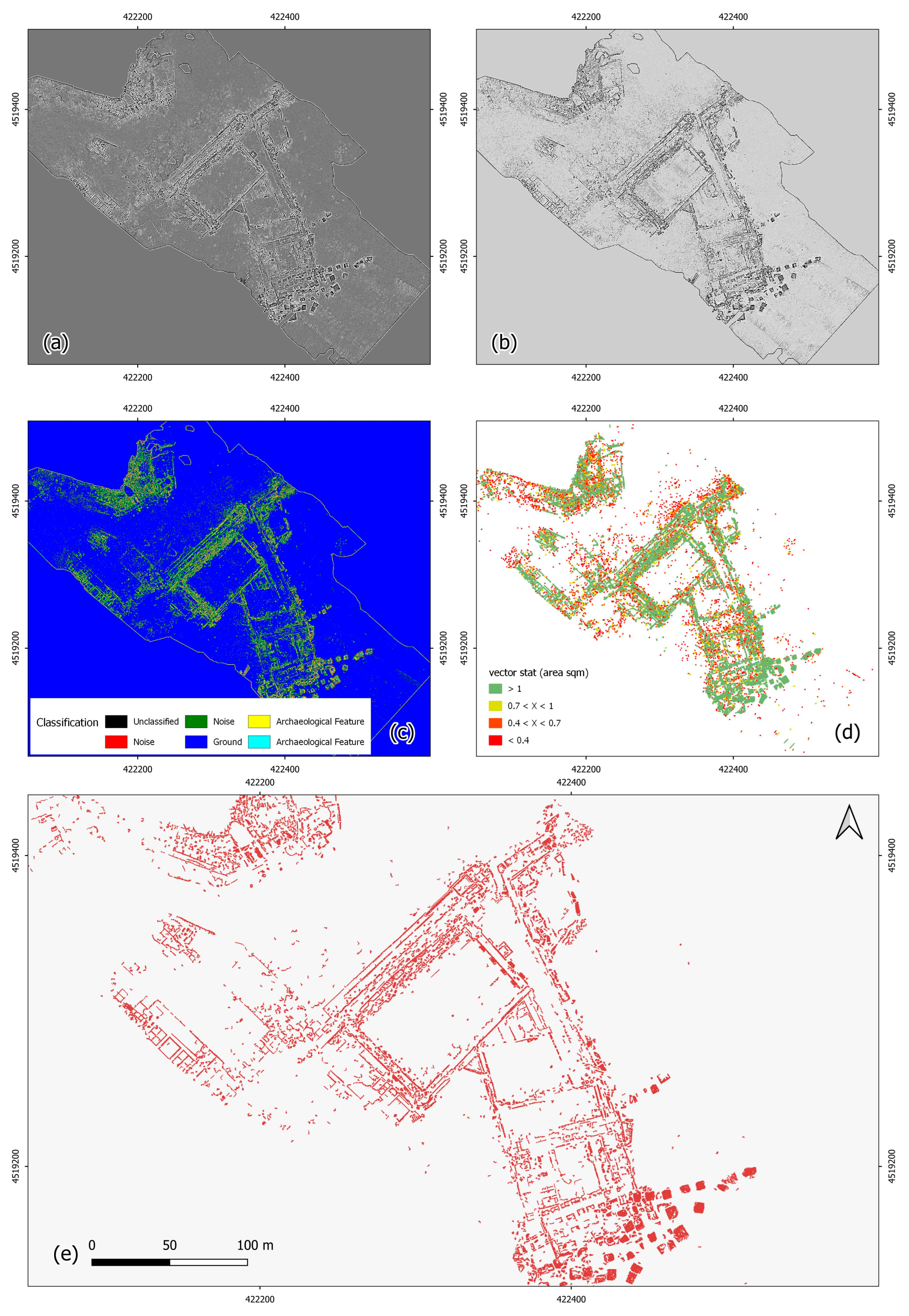
2.4. The Modified Automatic Feature Extraction Approach (MAFE)

Automatic archaeological feature extraction was achieved using a method created by Masini et al. [47,68,85], called AFE (Automatic Feature Extraction), slightly modified according to the principle of reducing input data before unsupervised classification.
The automatic feature extraction method used in this study is based on that used by Masini et al. [47,68], and aims to obtain a vector map that traces features of an archaeological nature in a semi-unsupervised way. The process is a machine-learning-based approach for semi-automatic feature extraction. It was based on the following steps: (i) selection of the input data from the DSM derivatives; (ii) data normalisation; (iii) data reduction; (iv) the extraction of zonal image statistics; (v) unsupervised classification; (vi) filtering; and (vii) classification evaluation.
For this analysis, the DSMs derived from the second group described in the previous section, i.e., those based on topographical parameters, were predominantly considered, as they are objectively more prone to automatic classification. The data used for the extraction of features of archaeological interest, among those produced by the DSM, were: (i) Slope Gradient (Slope); (ii) Simple Local Relief Model (SLRM); (iii) Sky-View Factor (SVF); (iv) Positive Openness (OP); (v) Negative Openness (ON); and Local Dominance (LD). These types of data was chosen because of all the derivatives produced, they are those that best identify topographical variations (e.g., cavities and convexities), as well as changes in slope and elevation.
In order to prepare the data for data reduction operations, a scaling normalisation of the data was applied, so that all values were in a standard range (e.g., between −1 and 1 or between 0 and 1) [86,87,88,89]. The data thus obtained were subjected to a data reduction operation through the use of a PCA (Principal Component Analysis) algorithm, in a variance–covariance matrix, in the software SAGA GIS v.9.2.0. PCA is a frequently used method for reducing data and their redundancy. This is based on reducing the amount of information in a few output data or organising the information in the output data, so as to have a variance–covariance or correlation scale, while preserving variability as much as possible [90,91,92]. As already discussed in other texts, particularly for the archaeological field, this procedure nevertheless presents risks of loss of information, especially in the case of small features [93]. PCA is a linear transformation that modifies the source data, transforming a number of correlated variables into a smaller number of uncorrelated variables but preserving most of the information in the input data, grouped into what are called components [94]. From the input bands, three main components were obtained. These were then analysed individually and in their RGB composition (R: 1st component, G: 2nd component, and B: 3rd component).
The most representative image for the purposes of the study was that of the second component, which, due to its characteristics, was subsequently subjected to a LISA (Local Indicator of Spatial Autocorrelation) type function in order to clusterise and further cleanse the data for classification.
These types of algorithms are applied to calculate the spatial autocorrelation of data. The indices used are (i) Moran’s index, (ii) Geary’s C index, and (iii) Getis–Ord G index [95,96,97], calculated according to [95,96]. A spatial autocorrelation analysis produces an enhanced image where pixels are grouped based on their correlation within a surrounding window, emphasising features that may not be readily apparent and minimising background noise, such as salt and pepper effects. The Getis–Ord G index, among the generated local spatial autocorrelation indices, was applied in the subsequent classification stage to identify and extract the features of interest.
The processed data were later employed for classification purposes. The procedures were involved the application of an unsupervised ISODATA (Iterative Self-Organizing Data Analysis Technique Algorithm) classifier. In the realm of remote sensing studies applied to archaeology, various unsupervised classifiers are utilized, including (i) the Kmeans clustering algorithm and (ii) the ISODATA (Iterative Self-Organizing Data Analysis) algorithm [98,99,100]. Unsupervised classification algorithms categorize pixels based on their inherent characteristics, such as spectral features, without requiring pre-existing training data. An unsupervised ISODATA classification based on five classes was used. The result of the classification was subsequently vectorised, transforming the raster into a vector, and geometric features (area and perimeter) were calculated for each polygon generated. The identification phase of features of archaeological interest was based on two principles: (i) removal of the background and (ii) feature cleaning on the basis of geometric characteristics (area). The (sandy) ground was removed, as it was identified by ISODATA as a single class. Subsequently, a principle based on the feature area was applied to remove the noise, which mainly consisted of natural and morphological elements in the scene (e.g., microdunes and marine vegetation). On the basis of the automatic distribution of values generated by QGIS during the visualisation phase, three useful classes were extracted for archaeological purposes, removing background noise: (i) areas greater than 1 m2; (ii) areas between 1 and 0.7 m2; and (iii) areas between 0.7 and 0.4 m2. These parameters were chosen because large structures (e.g., masonry work) exceed 1 m2 in area, while smaller areas refer to agglomerates of stones (presumably collapses of ancient structures) or scattered material (sparse blocks or stones).
Classification is a fundamental task in machine learning with widespread applications. To assess the outcomes of classification, it is essential to compare the assigned labels of a specific set of elements with the genuine (true) labels [101]. There are multiple ways of assessing the accuracy of a classification. These change depending on the data classified and the type of classifier (e.g., supervised and unsupervised) [102,103].
In order to evaluate the ISODATA classification, a ground truth dataset was subsequently created using the derived and improved DSMs, consisting of 553 randomly generated points via QGIS over the study area and in the shapefile generated by ISODATA, so that True Positives (TP), False Positives (FP), and False Negatives (FN) could be identified. These points were manually labelled into two classes: (i) archaeological features and (ii) non-archaeological features.
The validation of the results was also supported by a series of underwater dives in situ, with the aim of optically identifying some of the points that emerged during the underwater remote sensing analyses.
Finally, the most commonly used metrics for classification evaluation, in the case of ground truth elements, were calculated: (i) accuracy, (ii) Confusion Matrix, (iii) precision, (iv) recall, and (v) F1-score [101,104].
Accuracy is a metric commonly used to evaluate the performance of a classification model. Accuracy measures the percentage of correct predictions out of the total number of predictions. KA is the accuracy score. NCP and NTP are the number of correct prediction and the total number of predictions, respectively. It can be calculated using the following formula (1):
K A = N C P N T P × 100
The Confusion Matrix (CM) is a table that is often used to describe the performance of a classification model on a set of data for which the true values are known. It provides a more detailed breakdown of the model’s predictions. The confusion matrix has four entries: (i) True Positive (TP): instances that were correctly predicted as positive; (ii) True Negative (TN): instances that were correctly predicted as negative; (iii) False Positive (FP): instances that were incorrectly predicted as positive (Type I error); and (iv) False Negative (FN): instances that were incorrectly predicted as negative (Type II error).
Precision (P) is the ratio of correctly predicted positive observations to the total predicted positives. It is a measure of how many of the predicted positive instances are actually positive. Where P is the precision score, TP and FP are the true positive and false positive prediction, respectively, according to (2):
P = T P T P + F P
Recall (R or Sensitivity) is the ratio of correctly predicted positive observations to all the actual positives. It is a measure of how many of the actual positive instances were correctly predicted. Where R is the recall score, TP and FN are the true positive and false negative prediction, respectively (3):
R = T P T P + F N
The F1-score is a metric that considers both precision and recall to provide a balanced measure of a model’s performance. It is particularly useful when dealing with imbalanced datasets (4):
F 1 = 2 × P r e c i s i o n × R e c a l l P r e c i s i o n + R e c a l l
Finally, the classification result was manually integrated using the derived DSMs and their fusion products.

3. Results and Discussion

The results obtained from the elaborations described above show how the approach used on multibeam data was useful in improving the visualisation of features of archaeological interest, as well as their automatic classification, in the context of an archaeological study of the seabed.
DSM enhancement techniques have certainly provided useful and suggestive images for identifying archaeological structures and separating them from other components of the seabed substrate or for understanding micro-topographies of archaeological interest (Figure 4).
The derived products were essential for automatic classification by unsupervised classifiers (MAFE). However, equally important was the PCA and data reduction operation, conducted prior to the LISA analysis and classification. Indeed, this reduced the data to be classified to one (second PC), which was further modified by the use of LISAs, in particular the Getis–Ord G index. The latter refined the sharpness of the data (hot-spot), further reducing the salt-and-pepper effect of the second PC and facilitating ISODATA.
The segmentation of the non-supervised classification and the cleaning of the data were also important. These latter steps were necessary to obtain good data, reducing residual noise and false positives (Figure 5).
Of the five classes created by ISODATA, two were selected and merged because they were considered as more representative of the elements of archaeological interest (Figure 5c, Archaeological Feature classes). KA reached a value of over 92.76%, consisting of a total of observed points (NTP) of 553 and a total of corrected observations of (NCP) of 513. P and R were equal to 0.95 and 0.90, respectively, and the F1-score was 0.92.
As has already been demonstrated in other studies, the approach of using derived DSMs and their modifications either on their own or as part of classifications for the segmentation of features of archaeological interest proved to be an optimal way of proceeding. In contrast to the simple DSM data without shading, the HS, MHS, and PCA DSMs created an initial 2.5D model that allowed to observe, and in some cases understand, the archaeological scenery in relation to the ground. The derived DSMs similarly highlighted several features such as changes in slope, elevated areas, or concavities, highlighting the presence of significant structures and topographic variations (Figure 4 and Figure 5). The automatic classification was certainly one of the results with the most informative potential from an archaeological point of view. The final data, cleared of noise, certainly provided an excellent basis for the study of the archaeological area. In fact, the classification showed high-precision and -accuracy results, albeit with some missed classifications. The segmentation procedure resulted in a defined vector similar to a hand-made CAD drawing. This is useful at the same time as being a starting point for further vectorisation and integration, as well as a basis for initiating interpretative procedures based on archaeological knowledge of the context.

4. Conclusions

UHR MBES technology has recently proven to be one of the best techniques for mapping archaeological remains on the seabed [67]. However, in the field of the archaeological research of underwater heritage sites through remote sensing technologies, it is still an uncommon practice to try to automatically extract features of archaeological interest [34,65,67]. On the other hand, archaeologists who increasingly make use of this type of remotely sensed data are not always experts in complex processes and prefer to rely on autopsy interpretation. The MAFE (Modified Archaeological Feature Extraction) approach used herein has already been used in other above-ground contexts, in particular with data acquired from LiDAR for the analysis of sites under canopy [47,68,85]. This approach, applied to the UHR MBES data, which are similar to the output data returned by a LiDAR, provided very interesting and promising results for the archaeological research of underwater environments. Indeed, the results showed a good aptitude of this semi-automatic statistics and machine-learning-based approach to provide a map of archaeological features, similar to that which archaeologists usually produce autoptically using CAD- or GIS-based tools. In addition, the results showed a good aptitude of this semi-automatic approach based on statistics (e.g., PCA and LISA) and machine learning (e.g., ISODATA classification) to provide a map of archaeological features, with a good accuracy in classifying true positives and few false positives, as the tests in this work and others have shown (Table 2 and Table 3). In conclusion, MAFE applied to UHR MBES data has proven to be a valid support in and for the analysis of submerged sites, as in the case of the submerged city of Baia, providing an accurate and georeferenced vector map of features for use in CAD or GIS, graphically similar to what is required by archaeological research standards. The output data can also be used as the basis for autopsy-type archaeological analyses and to be integrated or modified manually.
The method used here has, of course, pros and cons compared to the manual extraction of features from the data.
Pros: (i) it is a replicable method that has already proven to be useful in different scenarios and with different types of data; (ii) although it is a semi-automatic extraction method not based on deep learning, it still has a very good discernment and classification accuracy; (iii) it is easy to use; (iv) it is fast to use; (v) it provides georeferenced files in vector and raster format; (vi) it can be modified and adapted as needed by setting the classification metric threshold to discriminate features; and (vii) it does not require over-performing hardware and can be carried out completely using open-source software.
Cons: (i) it still requires a minimum of basic knowledge in the use of GIS and image processing software (e.g., SAGA GIS and QGIS); (ii) compared to a fully manual classification, it is less accurate; (iii) compared to a fully manual classification, it provides less graphically ordered data (e.g., feature outlines that are less sharp than those that can be drawn manually); (iv) it does not allow for the separation of features that are connected to each other for which it provides a single feature vector (e.g., four walls of a room are represented as a quadrangular shape); (v) there is no interpretation of the data during vector creation, as might be performed by an archaeologist when drawing an archaeological map; (vi) features that are too small or only conceivable and microtopographic features that are intuitable but difficult to see are not identified and drawn; and (vii) it cannot represent features internal to large structures although visible to the eye (e.g., individual stones in a wall, pavements).
However, it is a method that is open to future developments, in accordance with recent research trends in the field of AI, such as (i) applying deep learning algorithms for linearising vector features to make the effect more similar to a manual product or (ii) using AI-based shape and image recognition to recognise the type of archaeological structure identified.

Author Contributions

Conceptualization, N.A., N.M. and C.V.; methodology, N.A., N.M. and C.V.; software, N.A. and C.V.; validation, N.A. and C.V.; formal analysis, N.A. and N.M.; investigation, C.V.; resources, C.V. and N.M.; data curation, N.A. and C.V.; writing—original draft preparation, N.A., N.M. and C.V.; writing—review and editing, N.A., N.M. and C.V.; visualization, N.A., N.M. and C.V.; supervision, C.V.; project administration, C.V. All authors have read and agreed to the published version of the manuscript.

Funding

This data acquisition and processing have been funded by Agreement between CNR and Baia Archaeological Park, DUS.AD017.108 Project, Technological innovation for the protection, valorization and protection of cultural heritage. The post-processing activity has been funded by RES Data Lab of CNR-ISPC and Project CHANGES—(Italian Ministry of University and Research—MUR).

Data Availability Statement

The original contributions presented in the study are included in the article, further inquiries can be directed to the corresponding author.

Acknowledgments

The authors would like to thank Fabio Pagano and Enrico Gallocchio of the Campi Flegrei Archaeological Park for logistical support; Samule Carannante of Marinesub, and Aleksandra Kruss and Paola Fabbretti of Norbit for technical support.

Conflicts of Interest

The authors declare no conflicts of interest.

References

  1. Otero, J. Heritage Conservation Future: Where We Stand, Challenges Ahead, and a Paradigm Shift. Glob. Chall. 2022, 6, 2100084. [Google Scholar] [CrossRef] [PubMed]
  2. Vu Hoang, K. The Benefits of Preserving and Promoting Cultural Heritage Values for the Sustainable Development of the Country. E3S Web Conf. 2021, 234, 00076. [Google Scholar] [CrossRef]
  3. Agapiou, A.; Lysandrou, V.; Hadjimitsis, D.G. Earth Observation Contribution to Cultural Heritage Disaster Risk Management: Case Study of Eastern Mediterranean Open Air Archaeological Monuments and Sites. Remote Sens. 2020, 12, 1330. [Google Scholar] [CrossRef]
  4. Agapiou, A.; Lysandrou, V.; Alexakis, D.D.; Themistocleous, K.; Cuca, B.; Argyriou, A.; Sarris, A.; Hadjimitsis, D.G. Cultural Heritage Management and Monitoring Using Remote Sensing Data and GIS: The Case Study of Paphos Area, Cyprus. Comput. Environ. Urban Syst. 2015, 54, 230–239. [Google Scholar] [CrossRef]
  5. Demetrescu, E.; Ferdani, D. From Field Archaeology to Virtual Reconstruction: A Five Steps Method Using the Extended Matrix. Appl. Sci. 2021, 11, 5206. [Google Scholar] [CrossRef]
  6. Moscato, V. Big Data in Cultural Heritage. In Encyclopedia of Big Data Technologies; Sakr, S., Zomaya, A., Eds.; Springer International Publishing: Cham, Switzerland, 2018; pp. 1–6. ISBN 978-3-319-63962-8. [Google Scholar]
  7. Poulopoulos, V.; Wallace, M. Digital Technologies and the Role of Data in Cultural Heritage: The Past, the Present, and the Future. Big Data Cogn. Comput. 2022, 6, 73. [Google Scholar] [CrossRef]
  8. Aznar, M.J. In Situ Preservation of Underwater Cultural Heritage as an International Legal Principle. J. Marit. Archaeol. 2018, 13, 67–81. [Google Scholar] [CrossRef]
  9. Prott, L. Underwater Cultural Heritage at Risk: Managing Natural and Human Impacts: REVIEWS. Int. J. Naut. Archaeol. 2007, 36, 429–431. [Google Scholar] [CrossRef]
  10. Pearson, N. Protecting and Preserving Underwater Cultural Heritage in Southeast Asia. In The Palgrave Handbook on Art Crime; Hufnagel, S., Chappell, D., Eds.; Palgrave Macmillan: London, UK, 2019; pp. 685–730. ISBN 978-1-137-54405-6. [Google Scholar]
  11. Secci, M. Survey and Recording Technologies in Italian Underwater Cultural Heritage: Research and Public Access within the Framework of the 2001 UNESCO Convention. J. Marit. Archaeol. 2017, 12, 109–123. [Google Scholar] [CrossRef]
  12. Trakadas, A.; Karra, A. Coastal Landscapes, Environmental Change, and Maritime Cultural Heritage Resources in Morocco: The Case Study of Essaouira. J. Marit. Archaeol. 2022, 17, 401–420. [Google Scholar] [CrossRef]
  13. Bruno, F.; Barbieri, L.; Muzzupappa, M.; Tusa, S.; Fresina, A.; Oliveri, F.; Lagudi, A.; Cozza, A.; Peluso, R. Enhancing Learning and Access to Underwater Cultural Heritage through Digital Technologies: The Case Study of the “Cala Minnola” Shipwreck Site. Digit. Appl. Archaeol. Cult. Herit. 2019, 13, e00103. [Google Scholar] [CrossRef]
  14. Scalercio, E.; Sangiovanni, F.; Gallo, A.; Barbieri, L. Underwater Power Tools for In Situ Preservation, Cleaning and Consolidation of Submerged Archaeological Remains. J. Mar. Sci. Eng. 2021, 9, 676. [Google Scholar] [CrossRef]
  15. Maarleveld, T.J.; Guérin, U.; Egger, B. Manual for Activities Directed at Underwater Cultural Heritage: Guidelines to the Annex of the UNESCO 2001 Convention; UNESCO: Paris, France, 2013; ISBN 978-92-3-001122-2. [Google Scholar]
  16. Tusa, S. Il Mare delle Egadi: Itinerari e Parchi Archeologici Subacquei; Regione Siciliana, Assessorato dei Beni Culturali e Ambientali e della Pubblica Istruzione, Dipartimento dei Beni Culturali e Ambientali e Dell’educazione Permanente: Palermo, Italy, 2005; ISBN 978-88-88559-22-3. [Google Scholar]
  17. Agizza, S. A Project Proposal for the Construction of Underwater Archaeological Nature Routes into the Protected Marine Area of Santa Maria Di Castellabate. Int. J. Environ. Geoinformatics 2015, 2, 49–55. [Google Scholar] [CrossRef]
  18. Papatheodorou, G.; Geraga, M.; Chalari, A.; Christodoulou, D.; Iatrou, M.; Fakiris, E.; Prevenios, M.; Ferentinos, G. Remote Sensing for Underwater Archaeology: Case Stud-Ies from Greece and Eastern Mediterranean. Bull. Geol. Soc. Greece 2017, 44, 100. [Google Scholar] [CrossRef]
  19. Luo, L.; Wang, X.; Guo, H.; Lasaponara, R.; Zong, X.; Masini, N.; Wang, G.; Shi, P.; Khatteli, H.; Chen, F.; et al. Airborne and Spaceborne Remote Sensing for Archaeological and Cultural Heritage Applications: A Review of the Century (1907–2017). Remote Sens. Environ. 2019, 232, 111280. [Google Scholar] [CrossRef]
  20. Westley, K. Satellite-Derived Bathymetry for Maritime Archaeology: Testing Its Effectiveness at Two Ancient Harbours in the Eastern Mediterranean. J. Archaeol. Sci. Rep. 2021, 38, 103030. [Google Scholar] [CrossRef]
  21. Deroin, J.-P.; Bou Kheir, R.; Abdallah, C. Geoarchaeological Remote Sensing Survey for Cultural Heritage Management. Case Study from Byblos (Jbail, Lebanon). J. Cult. Herit. 2017, 23, 37–43. [Google Scholar] [CrossRef]
  22. Cuca, B.; Hadjimitsis, D.G. Space Technology Meets Policy: An Overview of Earth Observation Sensors for Monitoring of Cultural Landscapes within Policy Framework for Cultural Heritage. J. Archaeol. Sci. Rep. 2017, 14, 727–733. [Google Scholar] [CrossRef]
  23. Casal, G.; Monteys, X.; Hedley, J.; Harris, P.; Cahalane, C.; McCarthy, T. Assessment of Empirical Algorithms for Bathymetry Extraction Using Sentinel-2 Data. Int. J. Remote Sens. 2019, 40, 2855–2879. [Google Scholar] [CrossRef]
  24. Cahalane, C.; Magee, A.; Monteys, X.; Casal, G.; Hanafin, J.; Harris, P. A Comparison of Landsat 8, RapidEye and Pleiades Products for Improving Empirical Predictions of Satellite-Derived Bathymetry. Remote Sens. Environ. 2019, 233, 111414. [Google Scholar] [CrossRef]
  25. McCarthy, J.; Benjamin, J. Multi-Image Photogrammetry for Underwater Archaeological Site Recording: An Accessible, Diver-Based Approach. J. Marit. Archaeol. 2014, 9, 95–114. [Google Scholar] [CrossRef]
  26. Drap, P. Underwater Photogrammetry for Archaeology. In Special Applications of Photogrammetry; Da Silva, D.C., Ed.; InTech: Nappanee, IN, USA, 2012; ISBN 978-953-51-0548-0. [Google Scholar]
  27. Semaan, L.; Salama, M.S. Underwater Photogrammetric Recording at the Site of Anfeh, Lebanon. In 3D Recording and Interpretation for Maritime Archaeology; McCarthy, J.K., Benjamin, J., Winton, T., van Duivenvoorde, W., Eds.; Springer International Publishing: Cham, Switzerland, 2019; pp. 67–87. ISBN 978-3-030-03635-5. [Google Scholar]
  28. Wright, A.E.; Conlin, D.L.; Shope, S.M. Assessing the Accuracy of Underwater Photogrammetry for Archaeology: A Comparison of Structure from Motion Photogrammetry and Real Time Kinematic Survey at the East Key Construction Wreck. J. Mar. Sci. Eng. 2020, 8, 849. [Google Scholar] [CrossRef]
  29. Ødegård, Ø.; Hansen, R.E.; Singh, H.; Maarleveld, T.J. Archaeological Use of Synthetic Aperture Sonar on Deepwater Wreck Sites in Skagerrak. J. Archaeol. Sci. 2018, 89, 1–13. [Google Scholar] [CrossRef]
  30. Janowski, L.; Kubacka, M.; Pydyn, A.; Popek, M.; Gajewski, L. From Acoustics to Underwater Archaeology: Deep Investigation of a Shallow Lake Using High-Resolution Hydroacoustics—The Case of Lake Lednica, Poland. Archaeometry 2021, 63, 1059–1080. [Google Scholar] [CrossRef]
  31. Menna, F.; Agrafiotis, P.; Georgopoulos, A. State of the Art and Applications in Archaeological Underwater 3D Recording and Mapping. J. Cult. Herit. 2018, 33, 231–248. [Google Scholar] [CrossRef]
  32. De Smet, T.S. Emerging Remote Sensing Methods in Underwater Archaeology. In New Directions in the Search for the First Floridians; University Press of Florida: Gainesville, FL, USA, 2019; pp. 221–240. ISBN 978-1-68340-073-8. [Google Scholar]
  33. Quinn, R. Acoustic Remote Sensing in Maritime Archaeology; Oxford University Press: Oxford, UK, 2011. [Google Scholar]
  34. Plets, R.; Quinn, R.; Forsythe, W.; Westley, K.; Bell, T.; Benetti, S.; McGrath, F.; Robinson, R. Using Multibeam Echo-Sounder Data to Identify Shipwreck Sites: Archaeological Assessment of the Joint Irish Bathymetric Survey Data: Using Multibeam Echo-Sounder Data to Identify Shipwreck Sites. Int. J. Naut. Archaeol. 2011, 40, 87–98. [Google Scholar] [CrossRef]
  35. Ødegård, Ø.; Sørensen, A.J.; Hansen, R.E.; Ludvigsen, M. A New Method for Underwater Archaeological Surveying Using Sensors and Unmanned Platforms. IFAC-Pap. 2016, 49, 486–493. [Google Scholar] [CrossRef]
  36. McCarthy, J.; Benjamin, J.; Winton, T.; van Duivenvoorde, W. The Rise of 3D in Maritime Archaeology. In 3D Recording and Interpretation for Maritime Archaeology; McCarthy, J.K., Benjamin, J., Winton, T., van Duivenvoorde, W., Eds.; Springer International Publishing: Cham, Switzerland, 2019; pp. 1–10. ISBN 978-3-030-03635-5. [Google Scholar]
  37. Bates, C.R.; Lawrence, M.; Dean, M.; Robertson, P. Geophysical Methods for Wreck-Site Monitoring: The Rapid Archaeological Site Surveying and Evaluation (RASSE) Programme: Evaluating Geophysical Methods for Wreck-Site Monitoring. Int. J. Naut. Archaeol. 2011, 40, 404–416. [Google Scholar] [CrossRef]
  38. Grządziel, A. Using Remote Sensing Data to Identify Large Bottom Objects: The Case of World War II Shipwreck of General von Steuben. Geosciences 2020, 10, 240. [Google Scholar] [CrossRef]
  39. Violante, C. Acoustic Remote Sensing for Seabed Archaeology. In Proceedings of the IMEKO TC4 International Conference on Metrology for Archaeology and Cultural Heritage, Trento, Italy, 22–24 October 2020; pp. 21–26. [Google Scholar]
  40. Gkionis, P.; Papatheodorou, G.; Geraga, M. The Benefits of 3D and 4D Synthesis of Marine Geophysical Datasets for Analysis and Visualisation of Shipwrecks, and for Interpretation of Physical Processes over Shipwreck Sites: A Case Study off Methoni, Greece. J. Mar. Sci. Eng. 2021, 9, 1255. [Google Scholar] [CrossRef]
  41. Papadopoulos, N. Shallow Offshore Geophysical Prospection of Archaeological Sites in Eastern Mediterranean. Remote Sens. 2021, 13, 1237. [Google Scholar] [CrossRef]
  42. Simyrdanis, K.; Papadopoulos, N.; Kim, J.; Tsourlos, P.; Moffat, I. Archaeological Investigations in the Shallow Seawater Environment with Electrical Resistivity Tomography. Surf. Geophys. 2015, 13, 601–611. [Google Scholar] [CrossRef]
  43. Nayak, N.; Nara, M.; Gambin, T.; Wood, Z.; Clark, C.M. Machine Learning Techniques for AUV Side-Scan Sonar Data Feature Extraction as Applied to Intelligent Search for Underwater Archaeological Sites. In Proceedings of the Field and Service Robotics, Zurich, Switzerland, 12–15 September 2017; Ishigami, G., Yoshida, K., Eds.; Springer: Singapore, 2021; pp. 219–233. [Google Scholar]
  44. Missiaen, T.; Sakellariou, D.; Flemming, N.C. Survey Strategies and Techniques in Underwater Geoarchaeological Research: An Overview with Emphasis on Prehistoric Sites. In Under the Sea: Archaeology and Palaeolandscapes of the Continental Shelf; Bailey, G.N., Harff, J., Sakellariou, D., Eds.; Springer International Publishing: Cham, Switzerland, 2017; pp. 21–37. ISBN 978-3-319-53160-1. [Google Scholar]
  45. Chang, R.; Wang, Y.; Hou, J.; Qiu, S.; Nian, R.; He, B.; Lendasse, A. Underwater Object Detection with Efficient Shadow-Removal for Side Scan Sonar Images. In Proceedings of the OCEANS 2016, Shanghai, China, 10–13 April 2016; pp. 1–5. [Google Scholar]
  46. Drap, P.; Papini, O.; Merad, D.; Pasquet, J.; Royer, J.-P.; Motasem Nawaf, M.; Saccone, M.; Ben Ellefi, M.; Chemisky, B.; Seinturier, J.; et al. Deepwater Archaeological Survey: An Interdisciplinary and Complex Process. In 3D Recording and Interpretation for Maritime Archaeology; McCarthy, J.K., Benjamin, J., Winton, T., van Duivenvoorde, W., Eds.; Springer International Publishing: Cham, Switzerland, 2019; pp. 135–153. ISBN 978-3-030-03635-5. [Google Scholar]
  47. Masini, N.; Abate, N.; Gizzi, F.T.; Vitale, V.; Minervino Amodio, A.; Sileo, M.; Biscione, M.; Lasaponara, R.; Bentivenga, M.; Cavalcante, F. UAV LiDAR Based Approach for the Detection and Interpretation of Archaeological Micro Topography under Canopy—The Rediscovery of Perticara (Basilicata, Italy). Remote Sens. 2022, 14, 6074. [Google Scholar] [CrossRef]
  48. Štular, B.; Eichert, S.; Lozić, E. Airborne LiDAR Point Cloud Processing for Archaeology. Pipeline and QGIS Toolbox. Remote Sens. 2021, 13, 3225. [Google Scholar] [CrossRef]
  49. Evans, D.H.; Fletcher, R.J.; Pottier, C.; Chevance, J.-B.; Soutif, D.; Tan, B.S.; Im, S.; Ea, D.; Tin, T.; Kim, S.; et al. Uncovering Archaeological Landscapes at Angkor Using Lidar. Proc. Natl. Acad. Sci. USA 2013, 110, 12595–12600. [Google Scholar] [CrossRef] [PubMed]
  50. Evans, D.; Traviglia, A. Uncovering Angkor: Integrated Remote Sensing Applications in the Archaeology of Early Cambodia. In Satellite Remote Sensing; Lasaponara, R., Masini, N., Eds.; Remote Sensing and Digital Image Processing; Springer: Dordrecht, The Netherlands, 2012; Volume 16, pp. 197–230. ISBN 978-90-481-8800-0. [Google Scholar]
  51. Mazza, D.; Parente, L.; Cifaldi, D.; Meo, A.; Senatore, M.R.; Guadagno, F.M.; Revellino, P. Quick Bathymetry Mapping of a Roman Archaeological Site Using RTK UAS-Based Photogrammetry. Front. Earth Sci. 2023, 11, 1183982. [Google Scholar] [CrossRef]
  52. Novak, A.; Poglajen, S.; Vrabec, M. Not Another Hillshade: Alternatives Which Improve Visualizations of Bathymetric Data. Front. Mar. Sci. 2023, 10, 1266364. [Google Scholar] [CrossRef]
  53. Kokalj, Ž.; Zakšek, K.; Oštir, K. Application of sky-view factor for the visualization of historic landscape features in lidar-derived relief models. Antiquity 2011, 85, 263–273. [Google Scholar] [CrossRef]
  54. Andersen, M.S.; Gergely, Á.; Al-Hamdani, Z.; Steinbacher, F.; Larsen, L.R.; Ernstsen, V.B. Processing and Performance of Topobathymetric LiDAR 2 Data for Geomorphometric and Morphological 3 Classification in a High-Energy Tidal Environment. Hydrol. Earth Syst. Sci. 2017, 21, 43–63. [Google Scholar] [CrossRef]
  55. Lecours, V.; Dolan, M.F.J.; Micallef, A.; Lucieer, V.L. A Review of Marine Geomorphometry, the Quantitative Study of the Seafloor. Hydrol. Earth Syst. Sci. 2016, 20, 3207–3244. [Google Scholar] [CrossRef]
  56. Wölfl, A.-C.; Snaith, H.; Amirebrahimi, S.; Devey, C.W.; Dorschel, B.; Ferrini, V.; Huvenne, V.A.I.; Jakobsson, M.; Jencks, J.; Johnston, G.; et al. Seafloor Mapping—The Challenge of a Truly Global Ocean Bathymetry. Front. Mar. Sci. 2019, 6, 434383. [Google Scholar] [CrossRef]
  57. De Natale, G.; Troise, C.; Pingue, F.; Mastrolorenzo, G.; Pappalardo, L.; Battaglia, M.; Boschi, E. The Campi Flegrei Caldera: Unrest Mechanisms and Hazards. Geol. Soc. Lond. Spec. Publ. 2006, 269, 25–45. [Google Scholar] [CrossRef]
  58. Lombardo, N. Baia: Le Terme Sommerse a Punta Dell’Epitaffio. Ipotesi Di Ricostruzione Volumetrica e Creazione Di Un Modello Digitale. Archeol. E Calc. 2009, 20, 373–396. [Google Scholar]
  59. Petriaggi, B.D.; Petriaggi, R.; Bruno, F.; Lagudi, A.; Peluso, R.; Passaro, S. A Digital Reconstruction of the Sunken “Villa Con Ingresso a Protiro” in the Underwater Archaeological Site of Baiae. IOP Conf. Ser. Mater. Sci. Eng. 2018, 364, 012013. [Google Scholar] [CrossRef]
  60. Bruno, F.; Gallo, A.; De Filippo, F.; Muzzupappa, M.; Davidde Petriaggi, B.; Caputo, P. 3D Documentation and Monitoring of the Experimental Cleaning Operations in the Underwater Archaeological Site of Baia (Italy). In Proceedings of the 2013 Digital Heritage International Congress (DigitalHeritage), Marseille, France, 28 October–1 November 2013; pp. 105–112. [Google Scholar]
  61. Davidde Petriaggi, B.; Stefanile, M.; Petriaggi, R.; Lagudi, A.; Peluso, R.; Di Cuia, P. Reconstructing a Submerged Villa Maritima: The Case of the Villa Dei Pisoni in Baiae. Heritage 2020, 3, 1199–1209. [Google Scholar] [CrossRef]
  62. Stefanile, M. Baia, Portus Julius and Surroundings. Diving in the Underwater Cultural Heritage in the Bay of Naples (Italy). In Proceedings of the 6th International Symposium on Underwater Research, Antalya-Kemer, Turkey, 17–20 May 2012; Oniz, H., Cicek, B., Eds.; pp. 28–47. [Google Scholar]
  63. Guth, P.L.; Van Niekerk, A.; Grohmann, C.H.; Muller, J.-P.; Hawker, L.; Florinsky, I.V.; Gesch, D.; Reuter, H.I.; Herrera-Cruz, V.; Riazanoff, S.; et al. Digital Elevation Models: Terminology and Definitions. Remote Sens. 2021, 13, 3581. [Google Scholar] [CrossRef]
  64. Wille, P.C. Sound Images of the Ocean in Research and Monitoring; Springer: Berlin/Heidelberg, Germany, 2005; ISBN 978-3-540-24122-5. [Google Scholar]
  65. Westley, K.; Quinn, R.; Forsythe, W.; Plets, R.; Bell, T.; Benetti, S.; McGrath, F.; Robinson, R. Mapping Submerged Landscapes Using Multibeam Bathymetric Data: A Case Study from the North Coast of Ireland: Mapping Submerged Landscapes Using Multibeam Bathymetric Data. Int. J. Naut. Archaeol. 2011, 40, 99–112. [Google Scholar] [CrossRef]
  66. Violante, C. A Geophysical Approach to the Fruition and Protection of Underwater Cultural Landscapes. Examples from the Bay of Napoli, Southern Italy. In La Baia di Napoli. Strategie per la Conservazione e la Fruizione del Paesaggio Culturale; ArtstudioPaparo: Napoli, Italy, 2023; pp. 64–71. [Google Scholar]
  67. Violante, C.; Gallocchio, E.; Pagano, F.; Papadopulos, N. Geophysical and Geoarchaeological Investigations in the Submerged Archaeological Park of Baia (South Italy). In Proceedings of the IMEKO TC—4 International Conference on Metrology for Archaeology and Cultural Heritage, Rome, Italy, 19–21 October 2023. [Google Scholar]
  68. Masini, N.; Gizzi, F.; Biscione, M.; Fundone, V.; Sedile, M.; Sileo, M.; Pecci, A.; Lacovara, B.; Lasaponara, R. Medieval Archaeology under the Canopy with LiDAR. The (Re)Discovery of a Medieval Fortified Settlement in Southern Italy. Remote Sens. 2018, 10, 1598. [Google Scholar] [CrossRef]
  69. Axelsson, P. DEM Generation from Laser Scanner Data Using Adaptive TIN Models. Int. Arch. Photogramm. Remote Sens. 2000, 33, 110–117. [Google Scholar]
  70. Van Kreveld, M. Digital Elevation Models and TIN Algorithms. In Algorithmic Foundations of Geographic Information Systems; van Kreveld, M., Nievergelt, J., Roos, T., Widmayer, P., Eds.; Lecture Notes in Computer Science; Springer: Berlin/Heidelberg, Germany, 1997; pp. 37–78. ISBN 978-3-540-69653-7. [Google Scholar]
  71. Lozić, E.; Štular, B. Documentation of Archaeology-Specific Workflow for Airborne LiDAR Data Processing. Geosciences 2021, 11, 26. [Google Scholar] [CrossRef]
  72. Lee, J.-S. Digital Image Enhancement and Noise Filtering by Use of Local Statistics. IEEE Trans. Pattern Anal. Mach. Intell. 1980, PAMI-2, 165–168. [Google Scholar] [CrossRef] [PubMed]
  73. Danese, M.; Gioia, D.; Vitale, V.; Abate, N.; Amodio, A.M.; Lasaponara, R.; Masini, N. Pattern Recognition Approach and LiDAR for the Analysis and Mapping of Archaeological Looting: Application to an Etruscan Site. Remote Sens. 2022, 14, 1587. [Google Scholar] [CrossRef]
  74. Kokalj, Ž.; Zakšek, K.; Oštir, K.; Pehani, P.; Čotar, K.; Somrak, M. Relief Visualization Toolbox; Version 2.0 Manual; ZRC SAZU: Ljubljana, Slovenije, 2019. [Google Scholar] [CrossRef]
  75. Challis, K.; Forlin, P.; Kincey, M. A Generic Toolkit for the Visualization of Archaeological Features on Airborne LiDAR Elevation Data. Archaeol. Prospect. 2011, 18, 279–289. [Google Scholar] [CrossRef]
  76. Hanus, K. The Applications of Airborne Laser Scanning in Archaeology. Stud. Anc. Art Civiliz. 2012, 16, 233–238. [Google Scholar]
  77. Devereux, B.J.; Amable, G.S.; Crow, P. Visualisation of LiDAR Terrain Models for Archaeological Feature Detection. Antiquity 2008, 82, 470–479. [Google Scholar] [CrossRef]
  78. Doneus, M.; Briese, C. Full-Waveform Airborne Laser Scanning as a Tool for Archaeological Reconnaissance. BAR Int. Ser. 2015, 1568, 99–106. [Google Scholar]
  79. Kokalj, Ž.; Hesse, R. Airborne Laser Scanning Raster Data Visualization; Prostor, Kraj, ČAS; ZRC SAZU, Založba ZRC: Ljubljana, Slovenije, 2017; Volume 14, ISBN 978-961-254-984-8. [Google Scholar]
  80. Zakšek, K.; Oštir, K.; Kokalj, Ž. Sky-View Factor as a Relief Visualization Technique. Remote Sens. 2011, 3, 398–415. [Google Scholar] [CrossRef]
  81. Abate, N.; Ronchi, D.; Vitale, V.; Masini, N.; Angelini, A.; Giuri, F.; Minervino Amodio, A.; Gennaro, A.M.; Ferdani, D. Integrated Close Range Remote Sensing Techniques for Detecting, Documenting, and Interpreting Lost Medieval Settlements under Canopy: The Case of Altanum (RC, Italy). Land 2023, 12, 310. [Google Scholar] [CrossRef]
  82. Yokoyama, R. Visualizing Topography by Openness: A New Application of Image Processing to Digital Elevation Models. Photogramm. Eng. 2022, 68, 257–266. [Google Scholar]
  83. Doneus, M. Openness as Visualization Technique for Interpretative Mapping of Airborne Lidar Derived Digital Terrain Models. Remote Sens. 2013, 5, 6427–6442. [Google Scholar] [CrossRef]
  84. Hesse, R. Visualisierung hochauflösender Digitaler Geländemodelle mit LiVT. In 3D-Anwendungen in der Archäologie. Berlin Studies of the Ancient World; Humboldt-Universität zu Berlin: Berlin, Germany, 2016. [Google Scholar] [CrossRef]
  85. Masini, N.; Lasaponara, R. On the Reuse of Multiscale LiDAR Data to Investigate the Resilience in the Late Medieval Time: The Case Study of Basilicata in South of Italy. J. Archaeol. Method Theory 2021, 28, 1172–1199. [Google Scholar] [CrossRef]
  86. Ahsan, M.M.; Mahmud, M.A.P.; Saha, P.K.; Gupta, K.D.; Siddique, Z. Effect of Data Scaling Methods on Machine Learning Algorithms and Model Performance. Technologies 2021, 9, 52. [Google Scholar] [CrossRef]
  87. Jo, J.-M. Effectiveness of Normalization Pre-Processing of Big Data to the Machine Learning Performance. J. Korea Inst. Electron. Commun. Sci. 2019, 14, 547–552. [Google Scholar] [CrossRef]
  88. Ali, P.J.M.; Faraj, R.H.; Koya, E.; Ali, P.J.M.; Faraj, R.H. Data Normalization and Standardization: A Technical Report. Mach. Learn. Tech. Rep. 2014, 1, 1–6. [Google Scholar] [CrossRef]
  89. Sola, J.; Sevilla, J. Importance of Input Data Normalization for the Application of Neural Networks to Complex Industrial Problems. IEEE Trans. Nucl. Sci. 1997, 44, 1464–1468. [Google Scholar] [CrossRef]
  90. Estornell, J.; Martí-Gavliá, J.M.; Sebastiá, M.T.; Mengual, J. Principal Component Analysis Applied to Remote Sensing. Model. Sci. Educ. Learn. 2013, 6, 83. [Google Scholar] [CrossRef]
  91. Hotelling, H. Analysis of a Complex of Statistical Variables into Principal Components. J. Educ. Psychol. 1933, 24, 417–441. [Google Scholar] [CrossRef]
  92. Abate, N.; Frisetti, A.; Marazzi, F.; Masini, N.; Lasaponara, R. Multitemporal–Multispectral UAS Surveys for Archaeological Research: The Case Study of San Vincenzo Al Volturno (Molise, Italy). Remote Sens. 2021, 13, 2719. [Google Scholar] [CrossRef]
  93. Agapiou, A. Enhancement of Archaeological Proxies at Non-Homogenous Environments in Remotely Sensed Imagery. Sustainability 2019, 11, 3339. [Google Scholar] [CrossRef]
  94. Lasaponara, R.; Masini, N. Preserving the Past from Space: An Overview of Risk Estimation and Monitoring Tools. In Sensing the Past; Masini, N., Soldovieri, F., Eds.; Geotechnologies and the Environment; Springer International Publishing: Cham, Switzerland, 2017; Volume 16, pp. 61–88. ISBN 978-3-319-50516-9. [Google Scholar]
  95. Anselin, L. Local Indicators of Spatial Association—LISA. Geogr. Anal. 1995, 27, 93–115. [Google Scholar] [CrossRef]
  96. Ord, J.K.; Getis, A. Local Spatial Autocorrelation Statistics: Distributional Issues and an Application. Geogr. Anal. 1995, 27, 286–306. [Google Scholar] [CrossRef]
  97. Srinivasan, S. Local and Global Spatial Statistics. In Encyclopedia of GIS; Shekhar, S., Xiong, H., Eds.; Springer: Boston, MA, USA, 2008; p. 615. ISBN 978-0-387-30858-6. [Google Scholar]
  98. Jensen, J.R. Introductory Digital Image Processing: A Remote Sensing Perspective; Pearson series in geographic information science; Pearson Education, Inc.: Glenview, IL, USA, 2016; ISBN 978-0-13-405816-0. [Google Scholar]
  99. Canty, M.J. Image Analysis, Classification and Change Detection in Remote Sensing: With Algorithms for Python, 4th ed.; CRC Press/Taylor & Francis Group: Boca Raton, FL, USA, 2019; ISBN 978-1-138-61322-5. [Google Scholar]
  100. Parcak, S.H. Satellite Remote Sensing for Archaeology; Routledge: London, UK; New York, NY, USA, 2009; ISBN 978-0-415-44877-2. [Google Scholar]
  101. Gösgens, M.; Zhiyanov, A.; Tikhonov, A.; Prokhorenkova, L. Good Classification Measures and How to Find Them. In Proceedings of the Advances in Neural Information Processing Systems, Denver, CO, USA, 6–14 December 2021; Curran Associates, Inc.: Red Hook, NY, USA, 2021; Volume 34, pp. 17136–17147. [Google Scholar]
  102. Vujovic, Z. Classification Model Evaluation Metrics. Int. J. Adv. Comput. Sci. Appl. 2021, 12, 599–606. [Google Scholar] [CrossRef]
  103. Hossin, M.; Sulaiman, M.N. A Review on Evaluation Metrics for Data Classification Evaluations. Int. J. Data Min. Knowl. Manag. Process 2015, 5, 1–11. [Google Scholar] [CrossRef]
  104. Fiorucci, M.; Khoroshiltseva, M.; Pontil, M.; Traviglia, A.; Del Bue, A.; James, S. Machine Learning for Cultural Heritage: A Survey. Pattern Recognit. Lett. 2020, 133, 102–108. [Google Scholar] [CrossRef]
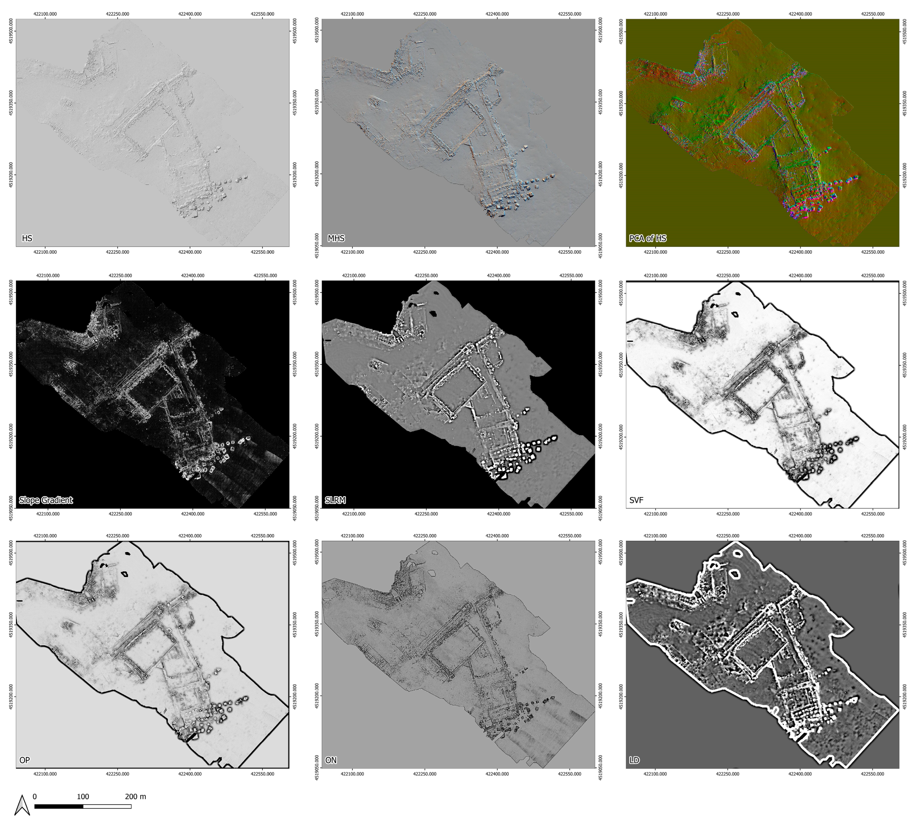
Figure 1. (a) Location of the AMP of Baia (dashed red line) with indication of the study area (red box); (b) Nymphaeum “Punta Epitaffio—Antonia Minore”; and (c) Portus Julius (this file is made available under the Creative Commons CC0 1.0 Universal Public Domain Dedication; Author: Ruthven).
Remotesensing 16 01908 g001
Figure 2. Flowchart.
Remotesensing 16 01908 g002
Figure 3. (a) DSM after applying Lee Filter (Reference System WGS84—EPSG::4326); (b) graph of DSM along segment A–B; and (c) graph of slope changes along segment A–B.
Remotesensing 16 01908 g003
Figure 4. DSM derivatives from RVT. In order from top left: HS, MHS, PCA of HS, Slope Gradient, SLRM, SVF, OP, ON, and LD.
Remotesensing 16 01908 g004
Figure 5. (a) Second PC, (b) Getis–ord Gi on second PC, (c) ISODATA classification, (d) selection of archaeological feature classes and calculation of geometric vector statistics, and (e) filtered archaeological map. The classification results obtained with the described methodologies are shown in Table 2 and Table 3.
Remotesensing 16 01908 g005
Table 1. Derivatives based on visualization techniques (RVT software v.2.2.1 desktop).
Visualization MethodParameters
Analytical Hill ShadingSun azimuth (deg): 315; Sun elevation angle (deg): 35
Hill Shading from Multiple DirectionsNumber of directions: 16; Sun elevation angle (deg): 35
PCA of Hill ShadingNumber of components to save: 3
Slope GradientNo parameters required
Simple Local Relief ModelRadius for trend assessment (pixel): 20 and 40
Sky-View FactorNumber of search directions: 16; search radius (pixel): 20 and 40
Openness PositiveNumber of search directions: 16; search radius (pixel): 20 and 40
Openness NegativeNumber of search directions: 16; search radius (pixel): 20 and 40
Local DominanceMinimum radius: 10 and 20; Maximum radius: 20 and 40
Table 2. Confusion Matrix.
CM
True Class
Predicted Class PositiveNegative
Positive27312
Negative28240
Table 3. Classification scores.
TypeScore
KA92.76%
P0.95
R0.90
F1-score0.92
Disclaimer/Publisher’s Note: The statements, opinions and data contained in all publications are solely those of the individual author(s) and contributor(s) and not of MDPI and/or the editor(s). MDPI and/or the editor(s) disclaim responsibility for any injury to people or property resulting from any ideas, methods, instructions or products referred to in the content.

