An Improved NLCS Algorithm Based on Series Reversion and Elliptical Model Using Geosynchronous Spaceborne–Airborne UHF UWB Bistatic SAR for Oceanic Scene Imaging

Abstract

Geosynchronous spaceborne–airborne (GEO-SA) ultra-high-frequency ultra-wideband bistatic synthetic aperture radar (UHF UWB BiSAR) provides high-precision images for marine and polar environments, which are pivotal in glacier monitoring and sea ice thickness measurement for polar ocean mapping and navigation. Contrasting with traditional high-frequency BiSAR, it faces unique challenges, such as the considerable spatial variability, significant range–azimuth coupling, and vast volumes of echo data, which impede high-resolution image reconstruction. This paper presents an improved bistatic nonlinear chirp scaling (NLCS) algorithm for imaging oceanic scenes with GEO-SA UHF UWB BiSAR. This methodology extends the two-dimensional (2-D) spectrum up to the sixth order via the method of series reversion (MSR) to meet accuracy demands and then employs an elliptical model to elucidate the alterations in the azimuth frequency modulation (FM) rate mismatch. Initially, the imaging geometry and signal model are introduced, and then a separation of bistatic slant ranges based on the configuration is proposed. In addition, during range processing, after eliminating linear range cell migration (RCM), the derivation process for the sixth-order 2-D spectrum is detailed and an improved filter is applied to correct the high-order RCM. Finally, during azimuth processing, the causes of the FM rate mismatch are analyzed, a cubic perturbation function derived from the elliptical model is used for FM rate equalization, and a unified sixth-order filter is applied to complete the azimuth compression. Experimental results with point targets and natural oceanic scenes validate the outstanding efficacy of the proposed NLCS algorithm, particularly in imaging quality enhancements for GEO-SA UHF UWB BiSAR.

1. Introduction

In the realm of contemporary marine remote sensing, synthetic aperture radar (SAR) systems play an indispensable role, spanning diverse applications such as polar ocean mapping and marine military target detection [1,2]. Distinguished from traditional optical and infrared sensors, SAR systems actively acquire high-resolution images, even in adverse environmental conditions [3]. Traditionally, SAR systems have been predominantly monostatic, characterized by their geometric simplicity and straightforward imaging algorithms. However, the trend in recent years has shifted towards bistatic and multi-static SAR systems, driven by their augmented information acquisition capabilities [4,5]. Simultaneously, due to the strong penetration capabilities of ultra-high-frequency (UHF) band signals, there is a growing interest in UHF ultra-wideband (UWB) SAR for detecting targets covered by ocean glaciers or foliage. On these foundations, geosynchronous spaceborne–airborne (GEO-SA) UHF UWB bistatic SAR (BiSAR) systems [6] are receiving increasing attention.

With the transmitter fixed on the GEO satellite and the passive receiver integrating into the airborne platform [7], the GEO-SA UHF UWB BiSAR system presents numerous advantages. One significant feature is the extraordinary orbit height of around 36,000 km, allowing for prolonged irradiation. Synchronized with the earth’s rotational velocity, the GEO satellite offers a revisit period of about 24 h, a significant improvement over the several-day periods of lower-orbit-altitude SAR systems [8,9]. The distant GEO satellite position ensures uninterrupted illumination for the passive and concealed receiver, enhancing its battlefield survivability in tasks like detecting maritime military targets. Additionally, the receiver’s flexible flight paths and UHF UWB signal enable comprehensive data acquisition [10]. In summary, the GEO-SA UHF UWB BiSAR system offers a multitude of advantages for marine remote sensing, including significantly reduced revisit periods, exceptional mobility and flexibility, a wide detection range, effective concealment capabilities, and impressive penetration capabilities. However, the characteristics of the “far-transmitting and near-receiving” geometry and UHF UWB signal pose some challenges for GEO-SA UHF UWB BiSAR image reconstruction, including complicated geometric configuration, large echo data volumes, considerable spatial variability, and significant range–azimuth coupling. Thus, it is imperative to engage in precise and efficient imaging research tailored to this kind of SAR system, and this indeed constitutes the central focus of this paper.

SAR imaging algorithms are generally classified into two main types: time domain and frequency domain algorithms. The former is widely applied for its superior imaging precision and adaptability to arbitrary-mode BiSAR. The backprojection (BP) algorithm [11] computes each pixel value by coherently summing each echo after precise phase compensation. Although the BP algorithm is suitable for the imaging of GEO-SA UHF UWB BiSAR, its pixel-by-pixel computation imposes a significant load. To alleviate this computational burden, the fast BP (FBP) algorithm [12] and the fast factorized BP (FFBP) algorithm [13] have been introduced. However, these algorithms still exhibit a significant efficiency gap compared to the frequency domain algorithms.

In arbitrary-mode BiSAR, the major challenge with frequency domain algorithms lies in the dual-root term of the instantaneous slant range, which complicates acquiring the precise analytical solutions applying the principle of stationary phase (POSP), adversely affecting imaging quality for non-center-scene targets. To mitigate this, Loffeld’s bistatic formula (LBF) [14] and the method of series reversion (MSR) [15] were proposed. The MSR expands the bistatic slant range into a Taylor series and derives an analytic two-dimensional (2-D) spectrum via series reversion, paving the way for the development of various algorithms [16,17,18]. Wong et al. first introduced the nonlinear chirp scaling (NLCS) algorithm [19], which is adept at handling higher-order spatial variation. This makes it appropriate for high-squint BiSAR imaging. To balance the azimuth frequency modulation (FM) rates, Wong et al. integrated the MSR with NLCS by a cubic perturbation function, first applying it to arbitrary-mode BiSAR [17]. Subsequent studies analyzed the relationship between the bistatic slant range variation and azimuth position from a geometric perspective, leading to more accurate perturbation functions and enhanced azimuthal focusing for edge targets in large scenes with high-squint angles [20,21,22,23,24]. Notably, the elliptical model proposed by Zhong et al. provided a more intuitive approach, albeit with increased computational complexity [23]. Liang et al. applied an elliptical model to forward-looking BiSAR with parallel platform trajectories [24]. Furthermore, Li et al. introduced a method based on the Lagrange inversion theorem (LIT) for deriving the point target spectra, incorporating the NLCS algorithm [25]. The NLCS algorithm has also been extensively applied in spaceborne illuminator BiSAR imaging [26,27,28]. These studies provide valuable insights for our research; however, they predominantly operate in high frequencies, with limited exploration in UHF UWB BiSAR imaging.

In this study, the system characteristics of squint angles and UHF UWB signal are taken into consideration, and the NLCS algorithm is employed to focus on high-resolution GEO-SA UHF UWB BiSAR imaging. Since the amplitude of the spectrum obtained by MSR is inversely proportional to the signal frequency, UHF UWB signals make the spectrum require more phase terms to meet the accuracy requirements, which increases the difficulty of spectrum derivation. Diverging from the NLCS algorithm tailored for SAR systems working at a higher frequency, the proposed NLCS algorithm for UHF UWB SAR systems utilizes the MSR to extend the 2-D spectral analysis up to the sixth order to meet the accuracy requirements. First, to alleviate range–azimuth coupling, the linear range cell migration correction (LRCMC) is employed to eliminate linear range cell migration (LRCM), commonly referred to as “squint minimizing.” Subsequently, a bulk range curvature correction (BRCC) filter based on the sixth-order spectrum is employed to eliminate the remaining range cell curvature and the decoupling of the range and azimuth, which accomplishes range-direction processing. Following this, an elliptical model is introduced to understand the variation in the targets’ slant range relative to the azimuth position before and after the LRCMC, and a cubic perturbation function is used to equalize the azimuth FM rates. Finally, azimuth compression is achieved using a unified sixth-order filter, which can result in a focused, high-resolution GEO-SA UHF UWB BiSAR image.

The paper is structured as follows: Section 2 presents the system imaging geometric configuration and signal model for the GEO-SA UHF UWB BiSAR, including the computation for both transmitted and received slant ranges. A flowchart is outlined in Section 3.1. Section 3.2 details the range-direction processing, including the LRCMC, the deduction of the 2-D spectrum, and the BRCC filter for the high-order phase removal. Section 3.3 discusses the azimuth-direction processing, introducing the elliptical model and deriving a perturbation function for the azimuth FM rate equalization, followed by the azimuth compression. The analysis of errors and computational cost is presented in Section 3.4. Section 4 demonstrates imaging experiments for the point targets and oceanic scenes. The final section concludes this paper.

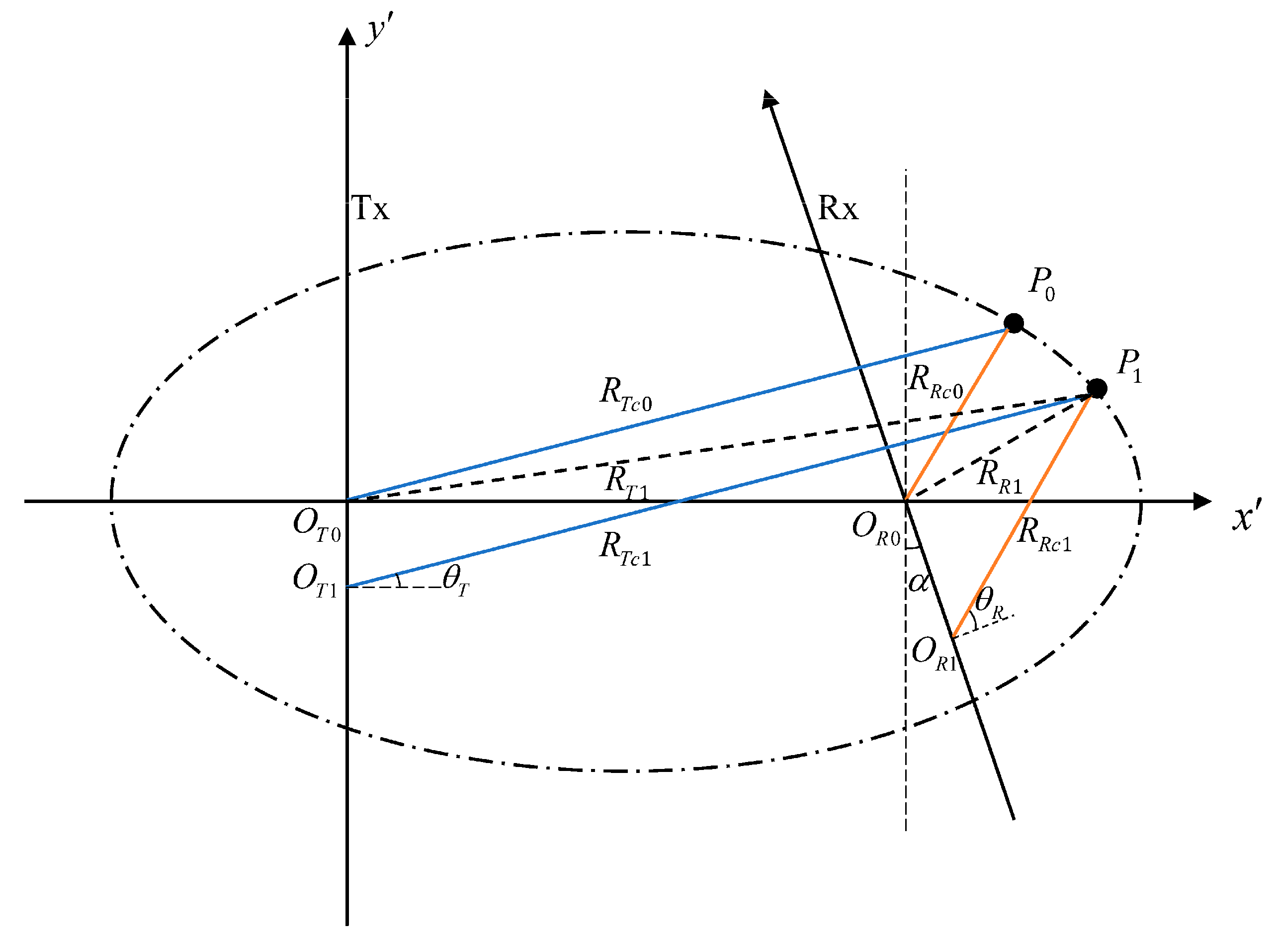
2. Geometric Configuration and Analysis

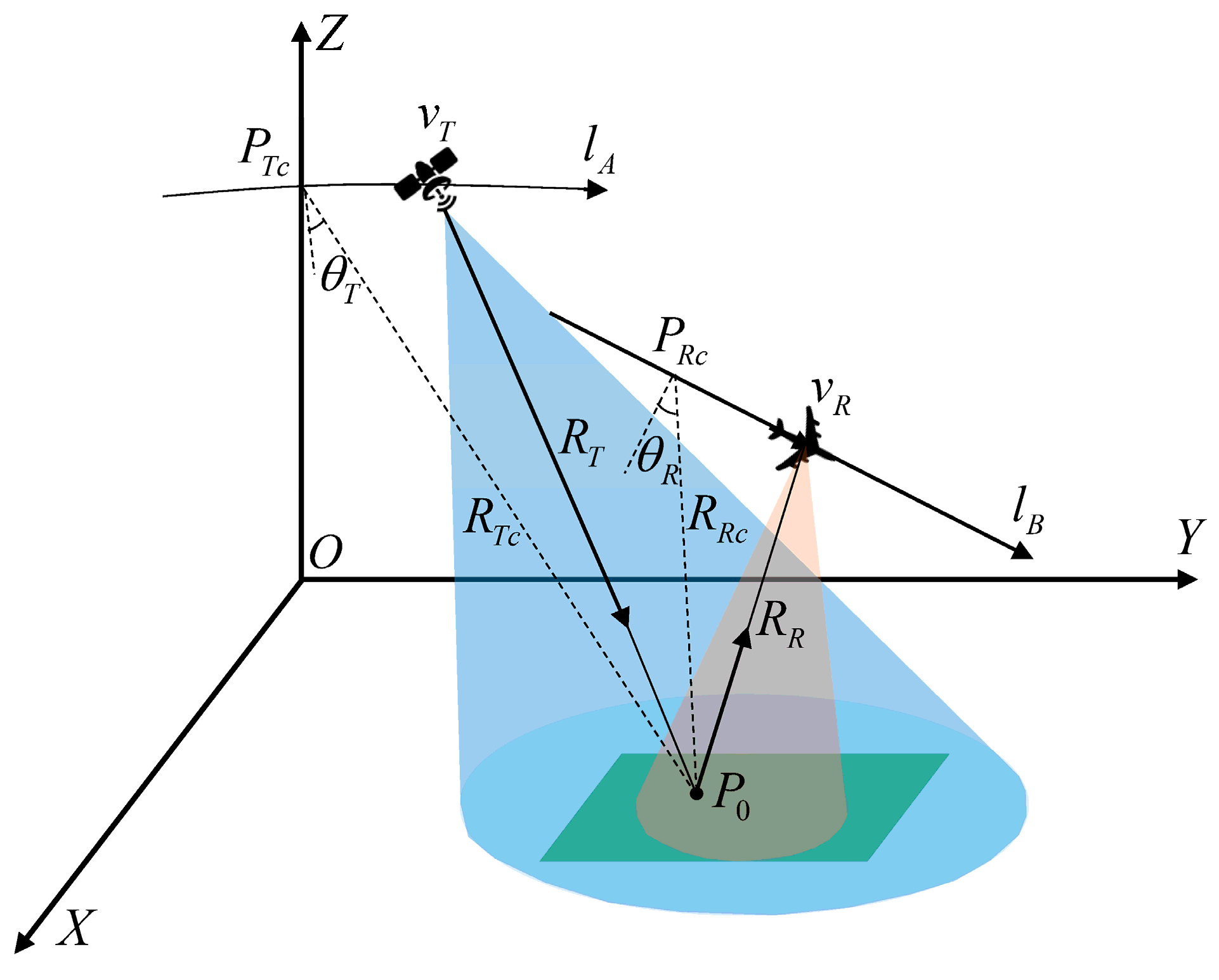
2.1. Imaging Geometric Configuration and Signal Model

Figure 1 illustrates the GEO-SA BiSAR imaging geometry, featuring the transmitter on a GEO satellite and the receiver on an airborne platform, with velocities of $v_T$ and $v_R$, respectively. $v_T$ and $v_R$ are non-parallel and their projection on the ground form an angle $\alpha$. The paths traced by the GEO satellite and receiver throughout the synthetic aperture period are represented as $l_A$ and $l_B$, respectively. At synthetic aperture center time ${\eta }_c$, their positions are $P_{Tc}$ and $P_{Rc}$, with $P_0$ indicating a reference target in the ground-imaging area. For simplification, the ground plane at $P_0$ is established as the $XOY$ plane in a Cartesian coordinate system, with $v_T$ aligned with the positive $Y$-axis direction, $P_{Tc}$ is at the positive $Z$-axis, and the $X$-axis orientation is ascertained by the right-hand rule. Considering the imaging area’s limited extent, the ground curvature is neglected. At an arbitrary azimuth time $\eta$, the respective transmitted and received slant ranges from the GEO satellite and receiver to a target in the scene are defined as:

$$\left\{\begin{array}{ll}{R}_T\left(\eta ;R_{Tc},{\eta }_c\right)& =\sqrt{R_{Tc}^2+v_T^2{\left(\eta -{\eta }_c\right)}^2-2v_T{R}_{Tc}\mathrm{s}\mathrm{i}\mathrm{n}{\theta }_T\left(\eta -{\eta }_c\right)}\\ R_R\left(\eta ;R_{Rc},{\eta }_c\right)& =\sqrt{R_{Rc}^2+v_R^2{\left(\eta -{\eta }_c\right)}^2-2v_R{R}_{Rc}\mathrm{s}\mathrm{i}\mathrm{n}{\theta }_R\left(\eta -{\eta }_c\right)}\end{array}\right.$$

(1)

where $R_{Tc}$ and $R_{Rc}$ represent the transmitted and received slant range at $\eta ={\eta }_c$, and ${\theta }_T$ and ${\theta }_R$ denote the squint angles of the two platforms, respectively. The instantaneous two-way slant range at azimuth time $\eta$ is presented as:

$$R_{bi}\left(\eta ;R_{bi0},{\eta }_c\right)=R_T\left(\eta ;R_{Tc},{\eta }_c\right)+R_R\left(\eta ;R_{Rc},{\eta }_c\right)$$

(2)

where $R_{bi0}$ represents the two-way slant range at $\eta ={\eta }_c$, which is calculated as:

$$R_{bi0}=R_{Tc}+R_{Rc}$$

(3)

Typically, the transmitted signal in GEO-SA BiSAR systems is a wideband linear frequency-modulated (LFM) signal. Thus, the demodulation signal is given as:

$$\begin{array}{ll}s\left(\tau ,\eta ;R_{bi0},{\eta }_c\right)& =w_r\left(\tau -\frac{R_{bi}\left(\eta ;R_{bi0},{\eta }_c\right)}{c}\right)w_a\left(\frac{\eta -{\eta }_c}{T_a}\right)\\ & \times \mathrm{e}\mathrm{x}\mathrm{p}\left(j\pi K_r{\left(\tau -\frac{R_{bi}\left(\eta ;R_{bi0},{\eta }_c\right)}{c}\right)}^2\right)\mathrm{e}\mathrm{x}\mathrm{p}\left(-j2\pi f_c\frac{R_{bi}\left(\eta ;R_{bi0},{\eta }_c\right)}{c}\right)\end{array}$$

(4)

where $\tau$ represents the fast time; $T_a$ is the synthetic aperture time; $f_c$ and $K_r$ correspond to the carrier frequency and the frequency chirp rate of the LFM signal, respectively; $c$ denotes the speed of light; and $w_r\left[\cdot \right]$ and $w_a\left[\cdot \right]$ are the range and azimuth envelopment fuctions, respectively. The echo signal, as presented in Equation (4), is transformed into the range frequency domain, which is carried out as:

$$S\left(f_{\tau },\eta ;R_{bi0},{\eta }_c\right)=W_r\left(f_{\tau }\right)w_a\left(\frac{\eta -{\eta }_c}{T_a}\right)\mathrm{e}\mathrm{x}\mathrm{p}\left(-j\pi \frac{f_{\tau }^2}{K_r}\right)\mathrm{e}\mathrm{x}\mathrm{p}\left(-j2\pi \frac{\left(f_{\tau }+f_c\right)}{c}{R}_{bi}\left(\eta ;R_{bi0},{\eta }_c\right)\right)$$

(5)

2.2. Separation of Slant Range Model

Due to the inherent characteristic of BiSAR, whose two-way slant range is a dual-root form, the direct application of the POSP to solve the precise analytical solution of the 2-D spectrum proves ineffective. Thus, the two-way slant range, as delineated in Equation (2), is expanded into a Taylor series as:

$$R_{bi}\left(\eta ;R_{bi0},{\eta }_c\right)=R_{bi0}+k_1\left(\eta -{\eta }_c\right)+k_2{\left(\eta -{\eta }_c\right)}^2+k_3{\left(\eta -{\eta }_c\right)}^3+o\left[{\left(\eta -{\eta }_c\right)}^n\right]$$

(6)

where the term $o\left[{\left(\eta -{\eta }_c\right)}^n\right]$ denotes higher-order components, while the expansion coefficients $k_n$ (for $n=\mathrm{1,2},3,\dots$) are calculated at the beam center crossing time $\eta ={\eta }_c$, specifically expressed as:

$$\begin{array}{ll}{k}_n& =k_{Tn}+k_{Rn}\\ & =\frac{1}{n!}\left(\frac{d^n{R}_T\left(\eta ;R_{Tc},{\eta }_c\right)}{d{\eta }^n}+\frac{d^n{R}_R\left(\eta ;R_{Rc},{\eta }_c\right)}{d{\eta }^n}\right){|}_{\eta ={\eta }_c}\end{array}$$

(7)

For the transmitter, the expansion coefficients for each order $k_{Tn}$ are given as:

$$\left\{\begin{array}{ll}{k}_{T1}& =-v_T\mathrm{s}\mathrm{i}\mathrm{n}{\theta }_T\\ k_{T2}& =\frac{v_T^2{\mathrm{c}\mathrm{o}\mathrm{s}}^2{\theta }_T}{2R_{Tc}}\\ k_{T3}& =\frac{v_T^3{\mathrm{c}\mathrm{o}\mathrm{s}}^2{\theta }_T\mathrm{s}\mathrm{i}\mathrm{n}{\theta }_T}{2R_{Tc}^2}\\ k_{T4}& =\frac{v_T^4{\mathrm{c}\mathrm{o}\mathrm{s}}^2{\theta }_T\left(4{\mathrm{s}\mathrm{i}\mathrm{n}}^2{\theta }_T-{\mathrm{c}\mathrm{o}\mathrm{s}}^2{\theta }_T\right)}{8R_{Tc}^3}\\ k_{T5}& =\frac{v_T^5{\mathrm{c}\mathrm{o}\mathrm{s}}^2{\theta }_T\left(9\mathrm{s}\mathrm{i}\mathrm{n}{\theta }_T-7\mathrm{s}\mathrm{i}\mathrm{n}3{\theta }_T\right)}{32R_{Tc}^4}\\ k_{T6}& =\frac{v_T^6{\mathrm{c}\mathrm{o}\mathrm{s}}^2{\theta }_T\left(15-28\mathrm{c}\mathrm{o}\mathrm{s}2{\theta }_T+21\mathrm{c}\mathrm{o}\mathrm{s}4{\theta }_T\right)}{128R_{Tc}^5}\end{array}\right.$$

(8)

In Equation (8), $k_{Tn}$ are retained up to the sixth order in preparation for the subsequent deduction for the 2-D spectrum of UHF UWB BiSAR. The expansion coefficients $k_{Rn}$ for the receiver are identical to $k_{Tn}$, with the only difference being the substitution of the subscript $T$ with $R$. Equation (8) indicates that the various-order coefficients are contingent only upon the center slant range, $R_{Tc}/R_{Rc}$, when the $v_T/v_R$ and ${\theta }_T/{\theta }_R$ are fixed. Distinct from monostatic SAR, BiSAR presents a more intricate geometric configuration, leading to the blurred definitions of the range and azimuth directions. Imaging is typically executed in the $\left(\tau -\eta \right)$ plane. In BiSAR, a fast time $\tau$ corresponds to a two-way slant range $R_{bi0}$. However, $R_{Tc}$ and $R_{Rc}$ are not simply in a proportional relationship. Therefore, it is imperative to calculate $R_{Tc}$ and $R_{Rc}$ separately based on the geometric configuration for each $R_{bi0}$ to subsequently solve for the expansion coefficients $k_n$ of $R_{bi0}$.

Figure 2a shows the simplified geometric imaging configuration of GEO-SA UHF UWB BiSAR. The GEO satellite, the receiver, and the reference target are positioned at the coordinates $P_{Tc}\left(\mathrm{0,0},h_T\right)$, $P_{Rc}\left(x_R,y_R,h_R\right)$, and $P_0\left(x_0,y_0,0\right)$, respectively, with $R_{T0}$ and $R_{R0}$ representing the minimum distances from the GEO satellite and receiver to the target $P_0$, respectively. The expression for the transmitted slant range is given as:

$$R_{Tc}=\frac{R_{T0}}{\mathrm{c}\mathrm{o}\mathrm{s}{\theta }_T}=\frac{\sqrt{x_0^2+h_T^2}}{\mathrm{c}\mathrm{o}\mathrm{s}{\theta }_T}$$

(9)

For the received slant range, the key is to ascertain the minimum ground distance $R_{RG}$ between the target and the receiver. Figure 2b delineates the geometric projection of the receiver’s trajectory $l_B$ onto the $XOY$ plane, where $l_{BG}$ and $P_{RG}$ represent the ground projections of $l_B$ and $P_{Rc}$, respectively. Based on geometric relationships, the following relationship is established:

$$R_{Rc}=\frac{R_{R0}}{\mathrm{c}\mathrm{o}\mathrm{s}{\theta }_R}=\frac{\sqrt{R_{RG}^2+h_R^2}}{\mathrm{c}\mathrm{o}\mathrm{s}{\theta }_R}$$

(10)

where

$$R_{RG}=\left[\left(x_0-x_R\right)-\left(y_0-y_R\right)\mathrm{t}\mathrm{a}\mathrm{n}\alpha \right]\mathrm{c}\mathrm{o}\mathrm{s}\alpha$$

(11)

By integrating Equations (3) and (9)–(11), $R_{Tc}$ and $R_{Rc}$ can be deduced from $R_{bi0}$.

3. Proposed Imaging Algorithm

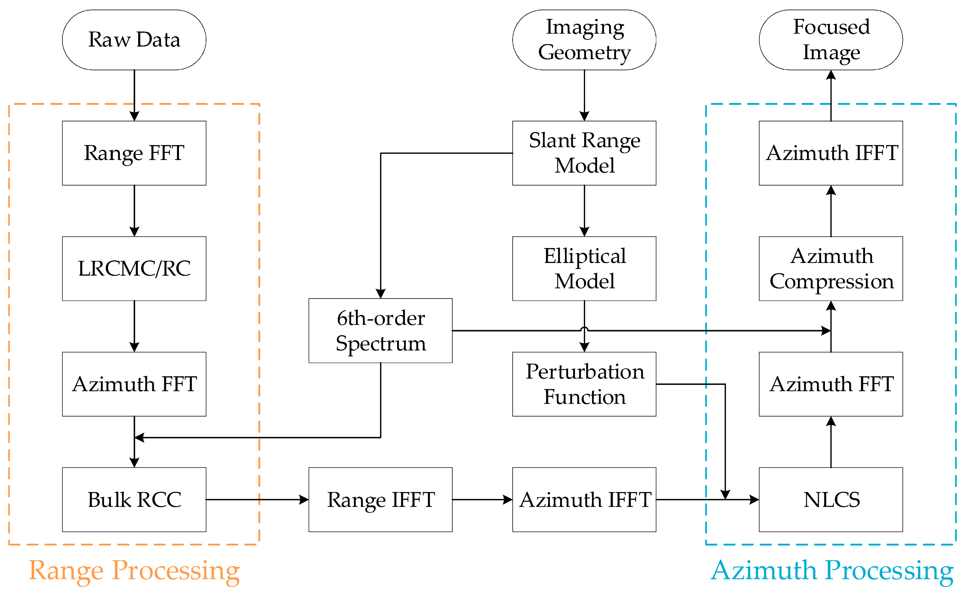
3.1. Description of the Proposed Algorithm

Before delving into the detailed methodology of the proposed algorithm, a comprehensive flow chart is provided in Figure 3 for a clearer understanding of the entire process. The proposed algorithm is divided into range and azimuth processing, delineated within the orange and blue dashed boxes, respectively. Initially, a reference LRCMC is applied in the range frequency domain, aiming to eliminate the range cell migration (RCM) caused by squint angles. Subsequently, the range curvature is corrected by a BRCC filter in the 2-D frequency domain. Notably, this BRCC filter is derived from the sixth-order 2-D spectrum, offering enhanced precision over the third-order spectrum. The azimuth-processing stage involves employing a cubic perturbation function to standardize the azimuth FM rates across targets in an identical range gate, hence facilitating NLCS processing. Perturbation function coefficients are determined through an elliptical model, which clarifies how the azimuth FM rate changes correlate with the azimuth time. Different range gates require distinct elliptical model parameters, thus necessitating the use of a slant range separation model to calculate the transmitted and received slant ranges for each gate. After NLCS, the azimuth compression is executed in the Doppler domain, where a sixth-order Doppler spectrum is computed for more precise phase compensation. Finally, the signal is converted back to the 2-D time domain to produce the focused SAR image.

3.2. Range Processing

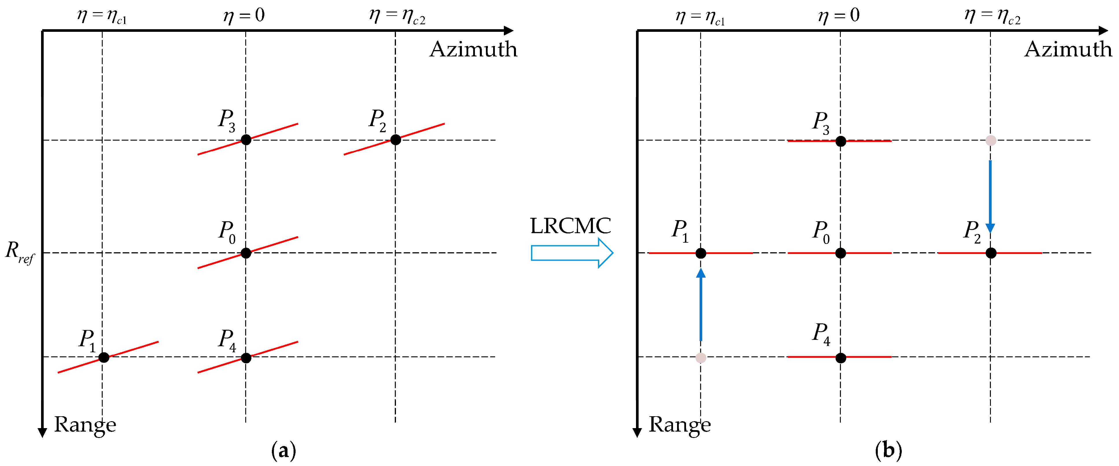
3.2.1. Linear Range Cell Migration Correction

The RCM can be divided into LRCM (first order) and nonlinear RCM (higher order). In the case of squinted BiSAR systems, LRCM dominates over the higher-order RCM, resulting in the sidelobes of point target impulse responses being non-parallel to the range and azimuth axes. Additionally, prior to employing the MSR for point target spectrum derivation, the LRCMC is imperative. This correction aims to remove the linear component from the two-way slant range $R_{bi}$, ensuring the resultant phase derivation is devoid of constant terms related to the azimuth time $\eta$, thereby streamlining the use of the MSR.

Figure 4 presents a diagram for the LRCMC in a squinted BiSAR setup, featuring five targets labeled $P_0$ to $P_4$ within the imaging scene. Due to the composite squint angle, targets $P_0$, $P_1$, and $P_2$ share an identical LRCM slope. Concurrently, $P_0$, $P_3$, and $P_4$ have a common beam center crossing time. Following the LRCMC, the first-order terms in the RCM of the five targets are removed, aligning their range migrations more closely with the azimuth time axis, as shown by the red lines in Figure 4. Furthermore, targets with the same LRCM slope will be relocated to the same range gate, as exemplified by $P_1$ and $P_2$ in the diagram. In arbitrary-mode BiSAR, an LRCMC filter can be effectively designed using the values at the reference target, such as the center of the imaging scene (illustrated by $P_0$ in Figure 4). The formulation of the filter is:

$$H_{LRCMC}\left(f_{\tau },\eta \right)=\mathrm{e}\mathrm{x}\mathrm{p}\left(j2\pi \frac{f_{\tau }+f_c}{c}{k}_1\eta \right)$$

(12)

To elucidate the impact of LRCMC, a simulation using parameters from

Table 1. Experimental parameters of GEO-SA UHF UWB BiSAR.

	Parameters	Values	Parameters	Values
BiSAR system	Center frequency	700 MHz	Bandwidth	150 MHz
	Pulse duration	1 μs	Sampling frequency	180 MHz
	PRF	172 Hz	Synthetic aperture time	7.08 s
GEO satellite	Orbital semi-major axis	42,164 km	Orbital eccentricity	0.006
	Initial coordinates	(0, 0, 35,753) km	Equivalent velocity	600 m/s
Receiver	Height	1000 m	X-axis velocity	40 m/s
	Squint angle	16°	Y-axis velocity	300 m/s
	Initial coordinates	(4000, 0, 1000) m	Angle $\alpha$	7.59°

is presented in Figure 5. Echoes from three point targets within the same range gate yet with distinct azimuth times are depicted in Figure 5a, with the central target designated as the LRCMC reference. The outcome is depicted in Figure 5b, where it is evident that the echo data support regions for the flanking targets have shifted, aligning approximately parallel to the azimuth time axis. Figure 5c and Figure 5d represent the 2-D spectra corresponding to Figure 5a and Figure 5b, respectively. Before LRCMC, point target spectra spread into adjacent channels, causing azimuth ambiguity. After LRCMC, the ambiguity disappears. It is noteworthy that the echo data support regions in Figure 5b and the spectra in Figure 5d are not rectangular, reflecting the substantial high-order RCM attributable to the UHF UWB signal, necessitating compensation in later stages. Additionally, before deriving the 2-D spectrum, range compression (RC) is required to eliminate range frequency modulation. The RC filter is defined as:

$$H_{RC}\left(f_{\tau },\eta \right)=\mathrm{e}\mathrm{x}\mathrm{p}\left(j\pi \frac{f_{\tau }^2}{K}\right)$$

(13)

By multiplying Equation (5) with Equations (12) and (13), we obtain the signal after the LRCM and RC, which is given by:

$$S_1\left(f_{\tau },\eta ;R_{bi0},{\eta }_c\right)=W_r\left(f_{\tau }\right)w_{\eta }\left(\frac{\eta -{\eta }_c}{T_a}\right)\mathrm{e}\mathrm{x}\mathrm{p}\left(-j2\pi \frac{\left(f_{\tau }+f_c\right)}{c}{R}_{bi}\mathrm{’}\left(\eta ;R_{bi0},{\eta }_c\right)\right)$$

(14)

where

$$\begin{array}{ll}{R}_{bi}\mathrm{’}\left(\eta ;R_{bi0},{\eta }_c\right)& =R_{bi0}-k_1{\eta }_c+k_2{\left(\eta -{\eta }_c\right)}^2+k_3{\left(\eta -{\eta }_c\right)}^3\\ & +k_4{\left(\eta -{\eta }_c\right)}^4+k_5{\left(\eta -{\eta }_c\right)}^5+k_6{\left(\eta -{\eta }_c\right)}^6+...\end{array}$$

(15)

3.2.2. Derivation of 2-D Spectrum and Bulk Range Curvature Correction

The derivation of the 2-D spectrum forms the foundation of frequency domain algorithms. Based on the preceding analysis, the direct application of the POSP is infeasible for computing the 2-D spectrum of arbitrary-mode BiSAR. To address this, the MSR is commonly employed to compute the spectrum, ensuring the accuracy by maintaining enough terms (typically until the phase of the last term is less than $\pi /4$). Existing research on MSR-based spectrum computation for arbitrary-mode BiSAR has predominantly focused on high-frequency systems with carrier frequencies above 5 GHz, where retaining three terms suffices for the accuracy. In contrast, low-frequency SAR, particularly in the UWB signal (0.3–1 GHz), necessitates retaining more terms for the accurate spectral computation, thereby increasing the computational complexity.

In this section, we proceed with the derivation of the 2-D spectrum for point targets. First, the azimuthal Fourier transform is applied on the range frequency spectrum as shown in Equation (14). By utilizing the POSP, we can obtain the 2-D spectrum of the point target, which is presented as:

$$\begin{array}{ll}S\left(f_{\tau },f_{\eta }\right)& =W_r\left(f_r\right)W_a\left(f_{\eta }\right)\mathrm{e}\mathrm{x}\mathrm{p}\left(j\Phi \left(f_{\tau },f_{\eta }\right)\right)\\ & =W_r\left(f_r\right)W_a\left(f_{\eta }\right)\mathrm{e}\mathrm{x}\mathrm{p}\left(-j2\pi \frac{\left(f_{\tau }+f_c\right)}{c}{R}_{bi}\mathrm{’}\left(\eta \left(f_{\eta }\right)\right)-j2\pi f_{\eta }\eta \left(f_{\eta }\right)\right)\end{array}$$

(16)

The azimuth frequency $f_{\eta }$, expressed in terms of the azimuth time $\eta$, is given by:

$$-\frac{c}{f_{\tau }+f_c}{f}_{\eta }=2k_2\left(\eta -{\eta }_c\right)+3k_3{\left(\eta -{\eta }_c\right)}^2+4k_4{\left(\eta -{\eta }_c\right)}^3+5k_5{\left(\eta -{\eta }_c\right)}^4+6k_6{\left(\eta -{\eta }_c\right)}^5$$

(17)

By the MSR, $f_{\eta }$ expressed as a function of $\eta$ is:

$$\eta -{\eta }_c=A_1\left(-\frac{c}{f_{\tau }+f_c}{f}_{\eta }\right)+A_2{\left(-\frac{c}{f_{\tau }+f_c}{f}_{\eta }\right)}^2+A_3{\left(-\frac{c}{f_{\tau }+f_c}{f}_{\eta }\right)}^3+A_4{\left(-\frac{c}{f_{\tau }+f_c}{f}_{\eta }\right)}^4+A_5{\left(-\frac{c}{f_{\tau }+f_c}{f}_{\eta }\right)}^5$$

(18)

where $A_i\left(i=\mathrm{1,2},3\cdots \right)$ are caculated as

$$\left\{\begin{array}{ll}{A}_1& =\frac{1}{2k_2}\\ A_2& =-\frac{3k_3}{8k_2^3}\\ A_3& =\frac{18k_3^2-8k_2{k}_4}{32k_2^5}\\ A_4& =-\frac{20k_2^2{k}_5-120k_2{k}_3{k}_4+135k_3^3}{128k_2^7}\\ A_5& =\frac{-48k_2^3{k}_6+360k_2^2{k}_3{k}_5+192k_2^2{k}_4^2-1512k_2{k}_3^2{k}_4+1134k_3^4}{512k_2^9}\\ & \cdots \end{array}\right.$$

(19)

Inserting Equation (18) into Equation (16) and expanding the phase as a series in powers of $f_{\eta }$, yields:

$$\Phi \left(f_{\tau },f_{\eta }\right)=-2\pi \frac{f_{\tau }+f_c}{c}(R_{bi0}-k_1{\eta }_c)-2\pi {\eta }_c{f}_{\eta }+2\pi C_n{\left(\frac{c}{f_{\tau }+f_c}\right)}^{n-1}{f}_{\eta }^n$$

(20)

where $n=\mathrm{2,3},4,\dots$, represent the orders of the point target’s 2-D spectrum, and $C_n$ corresponds to the coefficients for each order, specifically:

$$\left\{\begin{array}{ll}{C}_2& =\frac{1}{4k_2}\\ C_3& =\frac{k_3}{8k_2^3}\\ C_4& =\frac{9k_3^2-4k_2{k}_4}{64k_2^5}\\ C_5& =\frac{4k_2^2{k}_5-24k_2{k}_3{k}_4+27k_3^3}{128k_2^7}\\ C_6& =\frac{-8k_2^3{k}_6+32k_2^2{k}_4^2-252k_2{k}_3^2{k}_4+30k_2{k}_3{k}_5+189k_3^4}{512k_2^9}\\ & \cdots \end{array}\right.$$

(21)

It should be emphasized that the phase components diminish with increasing spectral order. Figure 6 presents simulated spectra for a GEO-SA UHF UWB BiSAR setup. The parameters for the simulation are presented in Table 1. It is evident that ${\varphi }_3>>\pi /4$, while ${\varphi }_6<<\pi /4$. Consequently, for GEO-SA UHF UWB BiSAR precision imaging, retaining merely up to the cubic terms in the spectrum proves inadequate, necessitating the preservation of up to the sixth-order terms for the subsequent steps of the algorithm.

Due to the longer wavelength of the UHF UWB signal, the high-order RCM remains significant even after LRCMC, requiring accurate compensation. the phase $\Phi \left(f_{\tau },f_{\eta }\right)$ is expanded into Taylor series at $f_{\tau }=0$ as:

$$\Phi \left(f_{\tau },f_{\eta };R_0\right)={\varphi }_0\left(f_{\eta }\right)+{\varphi }_1\left(f_{\eta }\right)f_{\tau }+{\varphi }_2\left(f_{\eta }\right)f_{\tau }^2+{\varphi }_3\left(f_{\eta }\right)f_{\tau }^3+...$$

(22)

where ${\varphi }_0\left(f_{\eta }\right)$ is independent of $f_{\tau }$ and represents the azimuth modulation term, which is:

$${\varphi }_0\left(f_{\eta };R_{0ref}\right)=-\frac{2\pi }{\lambda }{R}_{bi0}-2\pi {\eta }_c{f}_{\eta }+2\pi C_2\lambda f_{\eta }^2+2\pi C_3{\lambda }^2{f}_{\eta }^3+2\pi C_4{\lambda }^3{f}_{\eta }^4+2\pi C_5{\lambda }^4{f}_{\eta }^5+2\pi {C_6\lambda }^5{f}_{\eta }^6$$

(23)

In conventional high-frequency BiSAR systems, the range curvature correction (RCC) is generally adequate up to the cubic component. However, in UHF UWB BiSAR systems, the higher-order residual phase remains significant, rendering the cubic component compensation insufficient for precision requirements. In this paper, we employ an improved BRCC filter, which is defined as:

$$H_{BRCC}\left(f_{\tau },f_{\eta };R_{0ref}\right)=\mathrm{e}\mathrm{x}\mathrm{p}\left(-j\Phi \left(f_{\tau },f_{\eta };R_{0ref}\right)+j{\varphi }_0\left(f_{\eta };R_{0ref}\right)\right)$$

(24)

Multiplying Equation (24) by Equation (16) enables the elimination of all higher-order terms correlative to the range frequency, retaining only the terms independent of the range frequency and thus achieving the RCC. Notably, the application of the BRCC filter is under the assumption of an invariable range. In scenarios where the swath width is significantly large, a strategy involving dividing the swath along the range direction can be implemented.

3.3. Azimuth Processing

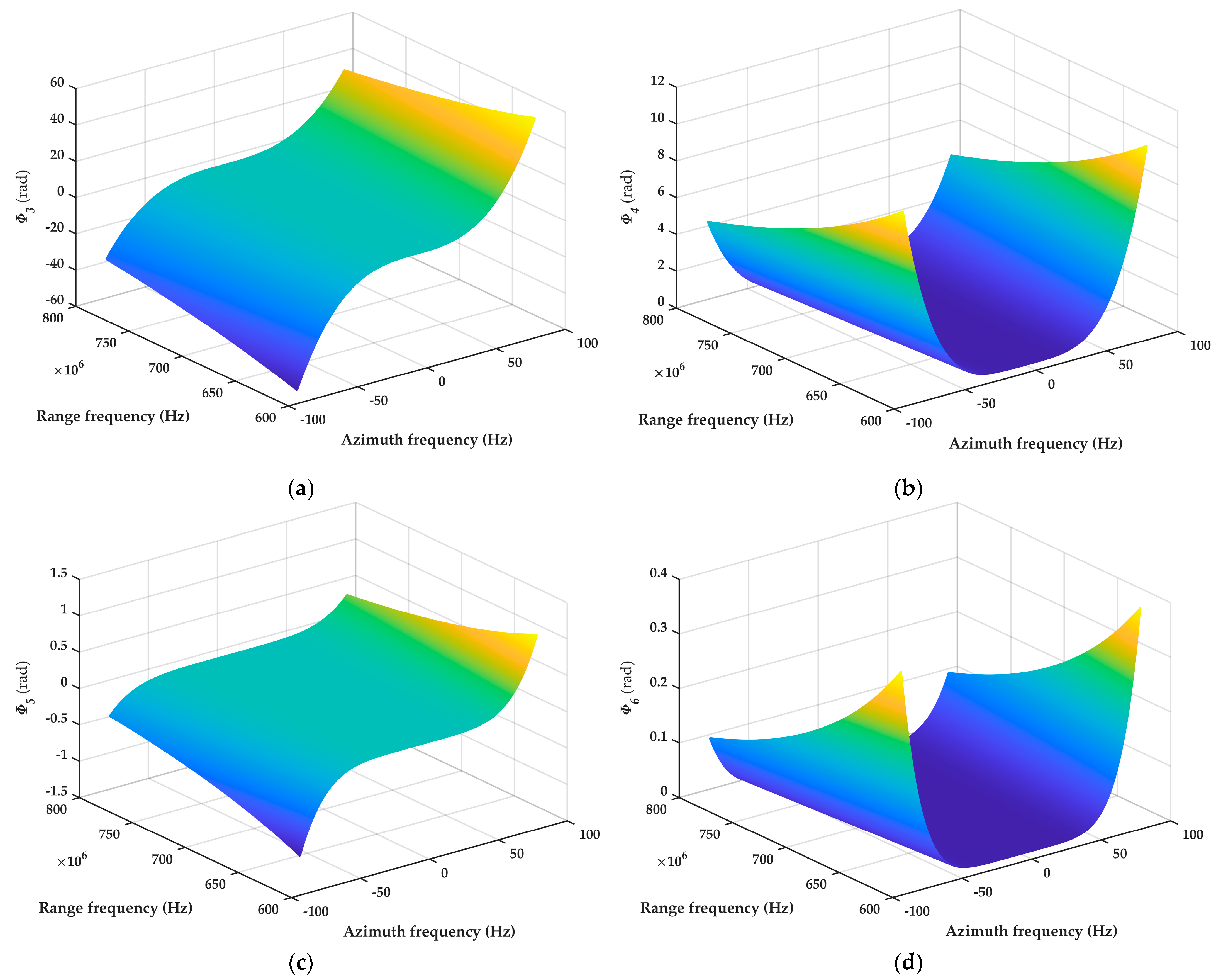
3.3.1. Analysis of FM Rate Distortion

After range processing, the point target’s spectrum depends solely on the azimuth frequency $f_{\eta }$. The phase is expanded into a Taylor series at $f_{\eta }=0$ as:

$$\psi \left(f_{\eta };R_{0ref}\right)\approx {\varphi }_0\left(f_{\eta };R_{0ref}\right)={\psi }_0+{\psi }_1{f}_{\eta }+{\psi }_2{f}_{\eta }^2+{\psi }_3{f}_{\eta }^3+{\psi }_4{f}_{\eta }^4+{\psi }_5{f}_{\eta }^5+{\psi }_6{f}_{\eta }^6$$

(25)

where ${\psi }_2$ is a function of $k_2$, which is correlative to the target’s azimuth FM rate. The azimuth FM rate can be given as:

$$K_a=-\frac{2k_2}{\lambda }=-\left(\frac{v_T^2{\mathrm{c}\mathrm{o}\mathrm{s}}^2{\theta }_T}{\lambda R_{Tc}}+\frac{v_R^2{\mathrm{c}\mathrm{o}\mathrm{s}}^2{\theta }_R}{\lambda R_{Rc}}\right)$$

(26)

As $v_T$, $v_R$, ${\theta }_T$, ${\theta }_R$, and $\lambda$ are all constant values, $K_a$ is only related to $R_{Tc}$ and $R_{Rc}$. In other words, targets in the same range gate share an identical $K_a$, which forms the basis for the azimuth compression. However, due to the effects of the LRCMC, targets undergo displacement along the range direction, leading to targets with identical LRCM slopes congregating in the same range gate. Nevertheless, these targets often have a different $K_a$, as demonstrated in Figure 7.

Taking the range gate $R_{ref}$, where $P_0$ is located as the reference, the targets’ FM rate in this range gate is denoted as $K_{aref}$. Before LRCMC, $P_1$ and $P_4$ are situated in the range gate $R_{+}$, sharing the identical FM rate $K_{a+}$, while $P_2$ and $P_3$ are situated in the range gate $R_{-}$, sharing the identical FM rate $K_{a-}$. After LRCMC, as $P_1$, $P_2$, and $P_0$ share the same LRCM slope, they converge within the same range gate. However, their FM rates persist unchanged despite the translation, with $P_1$, $P_0$, and $P_2$ maintaining respective FM rates of $K_{a-}$, $K_{aref}$, and $K_{a+}$.

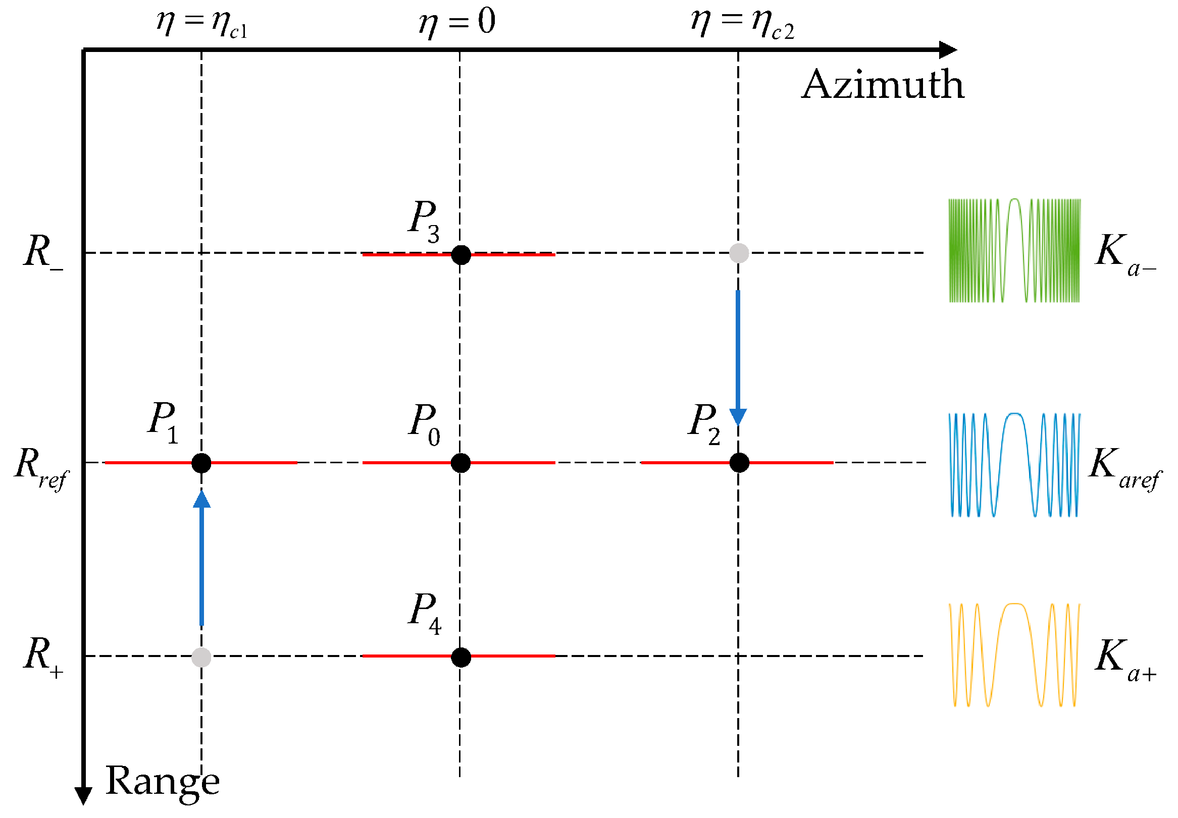
3.3.2. Elliptical Model and Perturbation Function

The azimuth FM rate mismatch prevents the application of a unified filter for the azimuth compression. Therefore, we introduce an elliptical model to quantify the azimuth FM rate mismatch and subsequently perform the equalization in the subsequent processing for a unified azimuth compression. To ascertain the targets’ FM rate within the identical range gate at varying azimuth times, determining their slant range before LRCMC is essential. An elliptical model is formulated, with the GEO satellite position $O_{T0}$ and the receiver position $O_{R0}$ at $\eta =0$ serving as the foci. The range gate $R_{ref}$ is set as the sum of a two-way slant range, as illustrated in Figure 8, leading to the following relationship:

$$\left\{\begin{array}{ll}2c_0& =\left|O_{T0}{O}_{R0}\right|\\ 2a_0& =R_{ref}=R_{Tc0}+R_{Rc0}\end{array}\right.$$

(27)

where $c_0$ and $a_0$ represent the semi-focal distance and semi-major axis of the ellipse, respectively, with $R_{Tc0}$ and $R_{Rc0}$ being the slant ranges of the two platforms to the reference point $P_0$. Considering $P_1$ as an example from Figure 7, at the instant $\eta ={\eta }_{c1}$, the positions of the GEO satellite and receiver are indicated as $O_{T1}$ and $O_{R1}$, respectively, satisfying $R_{+}=R_{Tc1}+R_{Rc1}$. After LRCMC, $P_1$ falls onto the same ellipse as $P_0$, where $R_{T1}+R_{R1}=R_{ref}=2a_0$. To investigate the slant range shifts of $P_1$ in relation to the azimuth time ${\eta }_{c1}$, $R_{Tc1}$, and $R_{Rc1}$ are expanded into a Taylor series at ${\eta }_{c1}=0$ and retain only the first-order terms, which produces the following expressions:

$$\left\{\begin{array}{ll}{R}_{Tc1}& =R_{Tc0}+\Delta R_T\approx R_{Tc0}+M{\eta }_{c1}\\ R_{Rc1}& =R_{Rc0}+\Delta R_R\approx R_{Rc0}+N{\eta }_{c1}\end{array}\right.$$

(28)

where

$$\left\{\begin{array}{ll}M& =\frac{a_0^2{v}_T\mathrm{s}\mathrm{i}\mathrm{n}{\theta }_T-a_0{c}_0{v}_T\mathrm{s}\mathrm{i}\mathrm{n}{\theta }_T\mathrm{c}\mathrm{o}\mathrm{s}{\theta }_T}{a_0^2+c_0^2{\mathrm{c}\mathrm{o}\mathrm{s}}^2{\theta }_T}\\ N& =\frac{v_R\mathrm{c}\mathrm{o}\mathrm{s}\alpha \left(-c_0+a_0\mathrm{c}\mathrm{o}\mathrm{s}{\theta }_R+a_0\mathrm{s}\mathrm{i}\mathrm{n}{\theta }_R\right)\left(a_0+c_0\mathrm{c}\mathrm{o}\mathrm{s}{\theta }_R\right)}{a_0^2+c_0^2{\mathrm{c}\mathrm{o}\mathrm{s}}^2{\theta }_R}\end{array}\right.$$

(29)

Notably, the traditional NLCS algorithm [17] directly considers the variation in the slant range as the shift in the LRCMC, i.e., $\Delta R_T+\Delta R_R\approx \left(v_T\mathrm{s}\mathrm{i}\mathrm{n}{\theta }_T+v_R\mathrm{s}\mathrm{i}\mathrm{n}{\theta }_R\right){\eta }_{c1}$. This approach collectively considers slant range variations, thereby overlooking the distinct impacts of transmitted and received slant ranges. Such a generalization lacks precision, especially for GEO-SA UHF UWB BiSAR with a large baseline. Additionally, by setting $R_{c0}=R_{Tc0}=R_{Rc0}$, $v=v_T=v_R$, and $\theta ={\theta }_T={\theta }_R$, the linear approximation relationship of slant ranges shown in Equation (28) reduces to the approximation of the monostatic SAR as $R_{c1}=R_{c0}+v\mathrm{s}\mathrm{i}\mathrm{n}\theta {\eta }_{c1}$.

Based on the preceding derivation, it is concluded that the difference in the targets’ azimuth FM rates within the identical range gate may be closely estimated to be a linear function of the azimuth time. Consequently, the perturbation function ought to take the form of a cubic equation in terms of azimuth time. the form of the perturbation function is assumed to be $H_{pert}=\mathrm{e}\mathrm{x}\mathrm{p}\left(j\pi {\alpha }_0{\eta }^3\right)$, where ${\alpha }_0$ is the perturbation coefficient, which will be further derived in the subsequent analysis.

Figure 9 illustrates the NLCS operation, with the cubic perturbation function represented by the orange curve in Figure 9a. Consider the three targets $P_0$, $P_1$, and $P_2$ in the reference range gate $R_{ref}$ from Figure 7. The differing azimuth FM rates of these targets before the perturbation result in varying rates of the phase change, as indicated by the quadratic curves with diverse curvatures. The perturbation function’s phase is then added to each target along the azimuth time, ensuring consistent azimuth FM rates for all targets. It is noteworthy that, except for the central target $P_0$, all other targets exhibit a unidirectional phase shift whose magnitude correlates with the azimuth time. This phase offset is due to the monotonicity of the perturbation function and results in a consistent magnitude of displacement in the positions of targets after azimuth compression, which can be easily removed through geometric correction subsequently [29]. To derive the values of the perturbation coefficients, take $P_1$ as an example. After introducing the perturbation function, the signals of targets $P_0$ and $P_1$ can be expressed as:

$$\begin{array}{ll}{S}_{pert0}\left(\tau ,\eta \right)=& S_0\mathrm{’}\left(\tau ,\eta \right)\mathrm{e}\mathrm{x}\mathrm{p}\left(j\pi {\alpha }_0{\eta }^3\right)\\ \hspace{1em}\hspace{1em}\hspace{1em}\hspace{1em} \approx & {\rho }_r\left(\tau -\frac{R_{ref}\left(\eta \right)}{c}\right)w_a\left(\eta \right)\mathrm{e}\mathrm{x}\mathrm{p}\left(j\pi {\alpha }_0{\eta }^3\right)\mathrm{e}\mathrm{x}\mathrm{p}\left[-j\frac{\pi }{\lambda }\left(\frac{v_T^2{\mathrm{c}\mathrm{o}\mathrm{s}}^2{\theta }_T}{R_{Tc0}}+\frac{v_R^2{\mathrm{c}\mathrm{o}\mathrm{s}}^2{\theta }_R}{R_{Rc0}}\right){\eta }^2\right]\end{array}$$

(30)

$$\begin{array}{ll}{S}_{pert1}\left(\tau ,\eta \right)=& S_1\mathrm{’}\left(\tau ,\eta \right)\mathrm{e}\mathrm{x}\mathrm{p}\left(j\pi {\alpha }_0{\eta }^3\right)\\ \hspace{1em}\hspace{1em}\hspace{1em}\hspace{1em} \approx & {\rho }_r\left(\tau -\frac{R_{ref}\left(\eta \right)}{c}\right)w_a\left(\eta -{\eta }_{c1}\right)\mathrm{e}\mathrm{x}\mathrm{p}\left(j\pi {\alpha }_0{\eta }^3\right)\mathrm{e}\mathrm{x}\mathrm{p}\left[-j\frac{\pi }{\lambda }\left(\frac{v_T^2{\mathrm{c}\mathrm{o}\mathrm{s}}^2{\theta }_T}{R_{Tc1}}+\frac{v_R^2{\mathrm{c}\mathrm{o}\mathrm{s}}^2{\theta }_R}{R_{Rc1}}\right){\left(\eta -{\eta }_{c1}\right)}^2\right]\end{array}$$

(31)

where $S_0\mathrm{’}\left(\tau ,\eta \right)$ and $S_1\mathrm{’}\left(\tau ,\eta \right)$ represent the 2-D time domain signals of targets $P_0$ and $P_1$ after the RC, respectively, and $p_r\left(\cdot \right)$ is the sinc function envelope. Since higher-order phases do not influence the first-order equilibrium of the azimuth FM rate, they are neglected here. By substituting Equation (28) into Equation (31) and then replacing $\left(\eta -{\eta }_{c1}\right)$ with ${\eta }_1$, Equation (31) can be rewritten as:

$$\begin{array}{ll}{S}_{pert1}\left(\tau ,\eta \right)\approx & {\rho }_r\left(\tau -\frac{R_{ref}\left(\eta \right)}{c}\right)w_a\left({\eta }_1\right)\\ & \times \mathrm{e}\mathrm{x}\mathrm{p}\left[j\pi {\alpha }_0\left({\eta }_1^3+3{\eta }_1^2{\eta }_{c1}+3{\eta }_1{\eta }_{c1}^2+{\eta }_{c1}^3\right)\right]\\ & \times \mathrm{e}\mathrm{x}\mathrm{p}\left[-j\frac{\pi }{\lambda }\left(\frac{v_T^2{\mathrm{c}\mathrm{o}\mathrm{s}}^2{\theta }_T}{R_{Tc0}}+\frac{v_R^2{\mathrm{c}\mathrm{o}\mathrm{s}}^2{\theta }_R}{R_{Rc0}}\right){\eta }_1^2\right]\\ & \times \mathrm{e}\mathrm{x}\mathrm{p}\left[-j\frac{\pi }{\lambda }\left(\frac{v_T^2{\mathrm{c}\mathrm{o}\mathrm{s}}^2{\theta }_T}{R_{Tc0}^2}M+\frac{v_R^2{\mathrm{c}\mathrm{o}\mathrm{s}}^2{\theta }_R}{R_{Rc0}^2}N\right){\eta }_{c1}{\eta }_1^2\right]\end{array}$$

(32)

To eliminate the terms correlating to the azimuth time ${\eta }_{c1}$ in the ${\eta }_1^2$ term, the expression for ${\alpha }_0$ is given by:

$${\alpha }_0=\frac{1}{3}\left(\frac{v_T^2{\mathrm{c}\mathrm{o}\mathrm{s}}^2{\theta }_T}{\lambda R_{Tc0}^2}M+\frac{v_R^2{\mathrm{c}\mathrm{o}\mathrm{s}}^2{\theta }_R}{\lambda R_{Rc0}^2}N\right)$$

(33)

3.3.3. Azimuth Compression

Once the perturbation function is applied, targets within the identical range gate attain uniform azimuth FM rates akin to the reference target, enabling the use of a unified filter for the azimuth compression. The time domain signal corresponding to the reference target $P_0$ after the range processing is represented as [17]:

$$S_0\left(\tau ,\eta \right)\approx {\rho }_r\left(\tau -\frac{R_{ref}\left(\eta \right)}{c}\right)w_a\left(\eta \right)\mathrm{e}\mathrm{x}\mathrm{p}\left(-j2\pi \frac{R_{ref}\left(\eta \right)}{\lambda }\right)$$

(34)

where $R_{ref}\left(\eta \right)$ signifies the instantaneous bistatic slant range of the reference target $P_0$. As per the previous analysis, to meet the imaging precision requirements in UHF UWB BiSAR systems, the instantaneous slant range here will be expanded into a Taylor series and retained up to the sixth-order term, expressed as:

$$R_{ref}\left(\eta \right)=R_{bi0}+k_2{\eta }^2+k_3{\eta }^3+k_4{\eta }^4+k_5{\eta }^5+k_6{\eta }^6$$

(35)

Multiplying with the perturbation function and then applying the azimuthal Fourier transform to Equation (34) yields:

$$\begin{array}{ll}{S}_{az0}\left(\tau ,f_{\eta }\right)=& \int {\rho }_r\left(\tau -\frac{R_{ref}\left(\eta \right)}{c}\right)w_a\left(\eta \right)\mathrm{e}\mathrm{x}\mathrm{p}\left(-j2\pi f_{\eta }\eta \right)\\ & \times \mathrm{e}\mathrm{x}\mathrm{p}\left[-j\frac{2\pi }{\lambda }\left(k_2{\eta }^2+k_3{\eta }^3+k_4{\eta }^4+k_5{\eta }^5+k_6{\eta }^6\right)+j\pi {\alpha }_0{\eta }^3\right]d\eta \end{array}$$

(36)

The constant phase term $\left(2\pi R_{bi0}/\lambda \right)$ in Equation (36) is neglected, as it bears no impact on the derivation of the azimuth compression filter. By employing the POSP, solving for the phase in Equation (36) with respect to the azimuth time $\eta$ and applying the MSR yields:

$$\begin{array}{ll}{f}_{\eta }\left(\eta \right)& =-\frac{1}{\lambda }\left(2k_2\eta +3k_3{\eta }^2+4k_4{\eta }^3+5k_5{\eta }^4+6k_6{\eta }^5\right)+\frac{3}{2}{\alpha }_0{\eta }^2\\ \eta \left(f_{\eta }\right)& =A_1{f}_{\eta }+A_2{f}_{\eta }^2+A_3{f}_{\eta }^3+A_4{f}_{\eta }^4+A_5{f}_{\eta }^5\end{array}$$

(37)

where

$$\left\{\begin{array}{ll}{A}_1& =+a_1^{-1}\\ A_2& =-a_1^{-3}{a}_2\\ A_3& =+a_1^{-5}\left(2a_2^2-a_1{a}_3\right)\\ A_4& =-a_1^{-7}\left(5a_2^3-5a_1{a}_2{a}_3+a_1^2{a}_4\right)\\ A_5& =+a_1^{-9}\left(14a_2^4-21a_1{a}_2^2{a}_3+3a_1^2{a}_3^2+6a_1^2{a}_2{a}_4-a_1^3{a}_5\right)\end{array}\right.$$

(38)

$$a_1=-\frac{2}{\lambda }{k}_2,a_2=\left(\frac{3}{2}{\alpha }_0-\frac{3}{\lambda }{k}_3\right),a_3=-\frac{4}{\lambda }{k}_4,a_4=-\frac{5}{\lambda }{k}_5,a_5=-\frac{6}{\lambda }{k}_6$$

(39)

By resolving the azimuth time $\eta$ from Equation (37) and substituting it back into Equation (36), the analytical expression for $S_{az0}\left(\tau ,f_{\eta }\right)$ is derived. The azimuth compression filter is then the complex conjugate of the phase in $S_{az0}\left(\tau ,f_{\eta }\right)$, which is given by:

$$H_{amf}\left(f_{\eta }\right)=\mathrm{e}\mathrm{x}\mathrm{p}\left[-j{\varphi }_{amf}\left(\eta \left(f_{\eta }\right)\right)\right]$$

(40)

where

$${\varphi }_{amf}\left(f_{\eta }\right)=-\frac{2\pi }{\lambda }\left(k_2{\eta }^2+k_3{\eta }^3+k_4{\eta }^4+k_5{\eta }^5+k_6{\eta }^6\right)+\pi {\alpha }_0{\eta }^3-2\pi f_{\eta }\eta \left(f_{\eta }\right)$$

(41)

Multiplying Equation (36) by Equation (40) eliminates the terms related to $f_{\eta }$ in the phase. Applying the azimuthal inverse Fourier transform yields the final focused image.

3.4. Analysis of the Proposed Algorithm

3.4.1. Error and Boundary Condition

From the preceding analysis, the error in the azimuth processing predominantly arises from the first-order approximation of the FM rate at non-reference points. Taking $P_1$ as an example again, we calculate its azimuth quadratic phase error (QPE). According to (26), the theoretical FM rate at $P_1$ is:

$$K_{a+}=-\left(\frac{v_T^2{\mathrm{c}\mathrm{o}\mathrm{s}}^2{\theta }_T}{\lambda R_{Tc1}}+\frac{v_R^2{\mathrm{c}\mathrm{o}\mathrm{s}}^2{\theta }_R}{\lambda R_{Rc1}}\right)$$

(42)

In the step of NLCS, the first-order approximation of the FM rate for $P_1$ is:

$$K_{a+}\mathrm{’}=-\left(\frac{v_T^2{\mathrm{c}\mathrm{o}\mathrm{s}}^2{\theta }_T}{\lambda R_{Tc0}}+\frac{v_R^2{\mathrm{c}\mathrm{o}\mathrm{s}}^2{\theta }_R}{\lambda R_{Rc0}}\right)+\left(\frac{v_T^2{\mathrm{c}\mathrm{o}\mathrm{s}}^2{\theta }_T}{\lambda R_{Tc0}^2}M+\frac{v_R^2{\mathrm{c}\mathrm{o}\mathrm{s}}^2{\theta }_R}{\lambda R_{Rc0}^2}N\right){\eta }_{c1}$$

(43)

Thus, the azimuth QPE at $P_1$ is:

$$QP{E}_{P_1}=\mathrm{m}\mathrm{a}\mathrm{x}\left\{\pi |K_{a+}-K_{a+}\mathrm{’}|{\left(\frac{T_a}{2}\right)}^2\right\}$$

(44)

The boundary condition $QPE<\pi /4$ integrating Equation (28), yields:

$$T_a<{\left[\frac{v_T^2\mathrm{c}\mathrm{o}\mathrm{s}{\theta }_T^2{M}^2{\eta }_{c1}^2}{\lambda \left(R_{T0}^3+R_{T0}^{2}M{\eta }_{c1}\right)}+\frac{v_R^2\mathrm{c}\mathrm{o}\mathrm{s}{\theta }_R^2{N}^2{\eta }_{c1}^2}{\lambda \left(R_{R0}^3+R_{R0}^{2}N{\eta }_{c1}\right)}\right]}^{-\frac{1}{2}}$$

(45)

Equation (45) indicates that $T_a$ and the azimuth position of the point target, ${\eta }_{c1}$, act as mutual constraints. $T_a$ decreases as ${\eta }_{c1}$ increases, while the azimuth resolution is directly proportional to $T_a$. Therefore, point targets located farther from the reference point exhibit lower azimuth resolution, which aligns with practical observations. In the imaging process, the size of the imaging scene can be derived from the desired resolution using Equation (45).

3.4.2. Computational Cost

The computational cost of the algorithm is primarily based on the times of FFTs, IFFTs, and complex multiplications performed during imaging processing. Typically, an N-point FFT or IFFT requires $5N{\mathrm{l}\mathrm{o}\mathrm{g}}_{2}N$ floating-point operations (FLOPs), and a N-point complex multiplication necessitates $6N$ FLOPs [30]. Wong’s traditional NLCS algorithm [17] utilizes four range FFTs or IFFTs, four azimuth FFTs or IFFTs, and five complex multiplications. Additionally, interpolation operations are needed when eliminating the residual RCM. According to the flowchart in Figure 3, the proposed method employs six FFTs or IFFTs and four complex multiplications, with no interpolation operations. Assuming that the samples in the range and azimuth directions are $N_r$ and $N_a$, respectively, and the kernel size for interpolation operations is $N_k$, the computational cost of Wong’s method and the proposed method can be calculated as follows:

$$C_{Wong}=20N_r{N}_a{\mathrm{l}\mathrm{o}\mathrm{g}}_2{N}_r+20N_r{N}_a{\mathrm{l}\mathrm{o}\mathrm{g}}_2{N}_a+30N_r{N}_a+2\left(2N_k-1\right)N_r{N}_a$$

(46)

$$C_{Proposed}=15N_r{N}_a{\mathrm{l}\mathrm{o}\mathrm{g}}_2{N}_r+15N_r{N}_a{\mathrm{l}\mathrm{o}\mathrm{g}}_2{N}_a+24N_r{N}_a$$

(47)

It is evident that the proposed method, in comparison to Wong’s method, decreases the computational operations required during data processing and avoids interpolation, leading to a substantial reduction in imaging time. This efficiency is particularly advantageous for real-time imaging of massive scenes. Moreover, regarding spectral accuracy, the only distinction between the proposed method with a spectrum of different orders lies in the application of more precise filters during BRCC and azimuth compression, not in increased computational steps. Consequently, achieving more accurate imaging results by increasing the order of the spectrum does not compromise the efficiency of the proposed method.

4. Experiment and Discussion

To validate the efficacy of the proposed algorithm, imaging experiments are conducted for point targets and natural scenes, with parameters detailed in Table 1. The radar operates in the UHF signal whose carrier frequency is 700 MHz and bandwidth is 150 MHz. With its relative bandwidth surpassing 20%, it qualifies as UHF UWB BiSAR. A BiSAR image is conducted using both the proposed NLCS algorithm and Wong’s traditional NLCS algorithm [17], which serves as a benchmark for comparison. Additionally, to assess the influence of spectral precision on imaging outcomes, the traditional NLCS algorithm retains the sixth-order spectrum, while the proposed NLCS algorithm is applied with spectra retained to both the third order and the sixth order, respectively. The imaging process excluded considerations such as the radio-frequency interference (RFI), Gaussian noise, electromagnetic wave propagation losses, etc. Additionally, to provide an objective evaluation of the effectiveness of each method, no window functions are utilized.

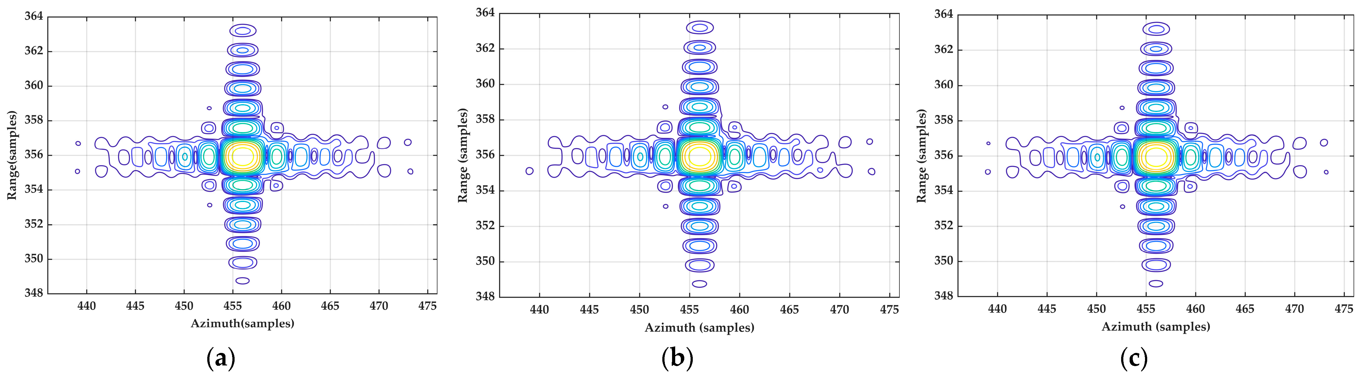
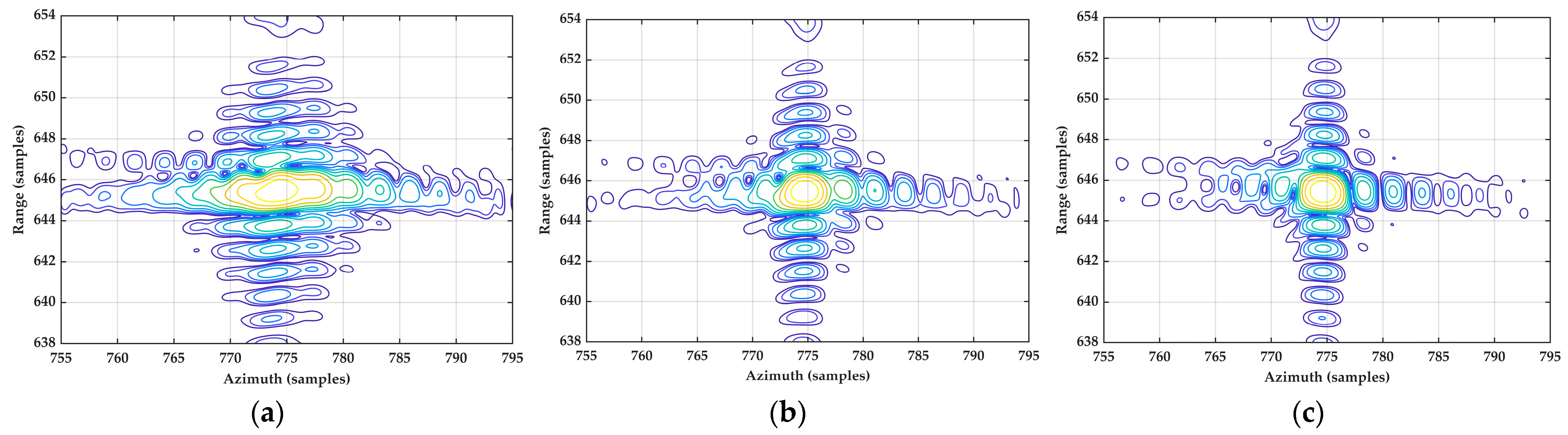
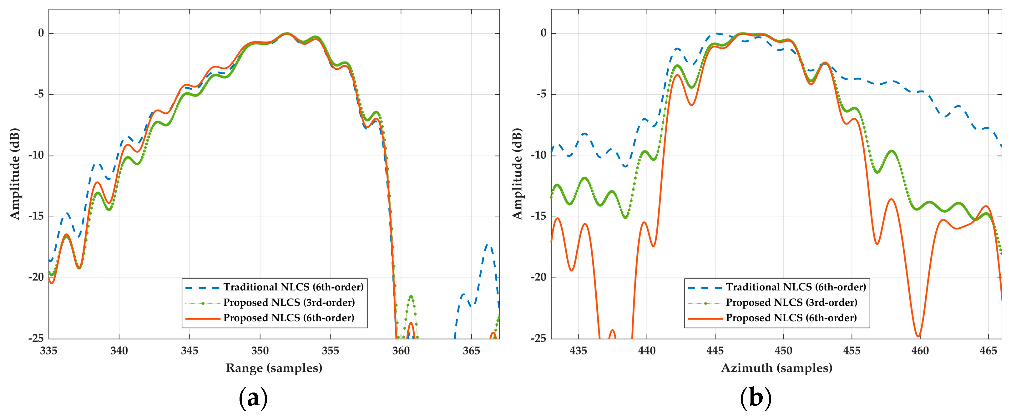
4.1. Experiment for Point Targets

In the experiment of point targets, 25 targets are strategically placed within the imaging scene, with the central target located at (14,000 m, 1500 m), designated as the reference target for the imaging. The other targets are systematically arranged with a separation of 200 m and 300 m in the range and azimuth direction, respectively, as presented in Figure 10a, while the focused imaging outcomes of the three approaches are presented in Figure 10b–d. Figure 10 confirms that all targets have been focused. However, the units in the imaging results are samples, because the geometric distortions occur along both the range and the azimuth dimension due to the effect of the squint angles. The omission of geometric correction maintains the primary sidelobes of targets aligned with the coordinate axes, aiding in precise parameter measurement of the targets.

To further compare the effectiveness of each method, three targets (P1, P13, P25) are selected for detailed analysis, where P13 is situated at the scene’s center, and P1 and P25 are positioned the farthest from the center. Contour maps illustrating the impulse responses for targets P1, P13, and P25 are exhibited in Figure 11, Figure 12 and Figure 13, respectively. To augment the detailed representation, each image result is subjected to an eightfold upsampling in both the range and the azimuth dimension.

Figure 11, Figure 12 and Figure 13 reveal that each target is well focused in the range direction. However, there is a disparity in azimuthal focus across the different methods. For the reference target P13, both the traditional NLCS algorithm and the proposed NLCS algorithm perform well. In contrast, for the edge targets P1 and P25, the azimuthal focusing performance of the traditional NLCS algorithm is significantly inferior to that of the proposed NLCS algorithm. Additionally, as indicated by the blue–purple contours in these figures, the azimuthal focusing performance is superior when the spectrum is retained up to the sixth order compared to retaining it up to the third order, irrespective of whether it is for the central target P13 or the peripheral targets P1 and P25.

Figure 14 illustrates the range and azimuth direction profiles of targets using three distinct methods: the traditional NLCS algorithm with the sixth-order spectrum (blue dashed line), the proposed NLCS algorithm with the third-order spectrum (green dotted line), and the proposed NLCS algorithm with the sixth-order spectrum (red solid line).

Table 2. Quantified IRW, PSLR, and ISLR of the selected targets.

		Range			Azimuth
		IRW (m)	PSLR (dB)	ISLR (dB)	IRW (m)	PSLR (dB)	ISLR (dB)
P1	Traditional NLCS (6th order)	0.99	−12.40	−9.73	5.75	−2.49	−4.71
	Proposed NLCS (3rd order)	1.00	−13.02	−10.65	2.09	−9.49	−8.18
	Proposed NLCS (6th order)	1.00	−13.42	−11.27	2.03	−13.63	−11.48
P13	Traditional NLCS (6th order)	1.00	−13.05	−10.42	2.12	−13.35	−11.00
	Proposed NLCS (3rd order)	1.00	−13.05	−10.43	2.13	−13.30	−10.73
	Proposed NLCS (6th order)	1.00	−13.05	−10.43	2.12	−13.36	−11.01
P25	Traditional NLCS (6th order)	1.03	−13.79	−11.25	3.24	−3.78	−5.80
	Proposed NLCS (3rd order)	1.00	−13.61	−11.23	2.34	−10.09	−8.82
	Proposed NLCS (6th order)	1.00	−13.38	−10.88	2.24	−13.10	−11.13

summarizes the impulse response width (IRW), peak sidelobe ratio (PSLR), and integrated sidelobe ratio (ISLR) of the three targets. The analysis from Figure 14 and Table 2 indicates that all targets exhibit sharp focusing within the range direction, and the focusing performance of the three methods is nearly identical and matches the theoretical IRW of 1 m. Moreover, the proposed NLCS algorithm with the sixth-order spectrum achieves the optimal focusing performance for the azimuth direction, with all targets exhibiting PSLR and ISLR below −13 dB and −10 dB, respectively. However, the traditional NLCS algorithm achieves good results only for the central target, while the focusing quality deteriorates significantly for the edge targets. The proposed NLCS algorithm with the third-order spectrum, with less precision, exhibits broadening in the main lobe, increased sidelobe levels, and reduced ISLR for the edge targets. Furthermore, asymmetrical azimuthal sidelobes in the impulse responses of the edge targets (Figure 14d,f) are observed due to the inadequate compensation of the higher-order spectral components.

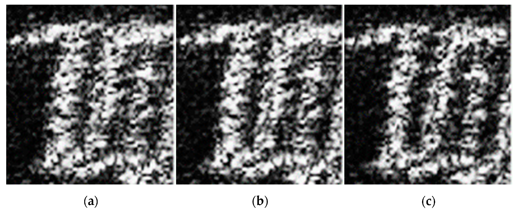
4.2. Experiment for Natural Oceanic Scenes

To further demonstrate the proposed algorithm’s efficacy, an experiment with a complex natural oceanic scene is conducted. Based on the target-by-target (TBT) method [31], natural scene echoes can be generated from SAR images by regarding pixel values as the electromagnetic scattering coefficients of the scene target, which is the so-called semi-real data. The natural scene image used for this experiment comprises 600 × 600 (range × azimuth) pixels [32]. The interval of each scatterer is set to one resolution cell, and detailed experimental parameters are provided in Table 1. The traditional NLCS algorithm with the sixth-order spectrum and the proposed NLCS algorithm with the third-order and sixth-order spectra are applied to process the TBT-generated echoes. Figure 15 displays the SAR image focused and geometrically corrected by the three methods. Due to the neglect of the separate influences of the transmitted and received slant ranges on the perturbation function in large-baseline BiSAR, the quality of imaging results obtained from the traditional NLCS algorithm is inferior, particularly in the edge regions. In contrast, the proposed NLCS algorithm employs an elliptical model to derive a more precise perturbation function, enhancing imaging quality in the scene’s edge areas.

For enhanced detail, Figure 16 zooms into the area marked by the red dashed rectangle (edge targets) in Figure 15a. The outcomes of Figure 16 illustrate that, in the azimuth direction, the traditional NLCS algorithm with the sixth-order spectrum performs the poorest, the proposed NLCS algorithm with the third-order spectrum fares better, and the NLCS algorithm with the sixth-order spectrum exhibits the best focusing performance. Similar to the point target experiments, Figure 17 presents the range and azimuth profiles for edge targets highlighted by red circles in Figure 15a. The range profiles of the three algorithms are comparable, but the traditional NLCS algorithm’s sidelobes are marginally elevated. In the azimuth direction, however, the traditional NLCS algorithm with the sixth-order spectrum shows the weakest focusing, characterized by sidelobe levels that surpass −10 dB. The proposed NLCS algorithm with the sixth-order spectrum matches the proposed NLCS algorithm with the third-order spectrum in the mainlobe focusing but achieves lower sidelobe levels and greater precision. Therefore, the traditional NLCS algorithm is unsuitable for the imaging of GEO-SA UHF UWB BiSAR, and thus, extending the spectrum to the sixth order is necessary for UHF band SAR imaging algorithms.

5. Conclusions

In this paper, an improved NLCS algorithm tailored for focusing on maritime scenes utilizing GEO-SA UHF UWB BiSAR is proposed. Diverging from the traditional high-frequency SAR, a third-order spectrum based on the MSR no longer meets the precision requirements. Therefore, we derive the 2-D spectrum up to the sixth order, until the phase of the highest-order spectrum is less than $\pi /4$. Based on this derived spectrum, an improved BRCC filter is employed to eliminate higher-order terms of RCM. During azimuth processing, an elliptical model is applied to illustrate the slant range’s variation with azimuth times, followed by employing a third-order perturbation function for azimuth FM rate equalization. Ultimately, a sixth-order azimuth compression filter is applied to complete the azimuthal focusing for the sixth-order spectra. Experimental results involving both point targets and maritime scenes affirm the proposed algorithm’s effectiveness. Compared to the traditional NLCS algorithm, the improved NLCS algorithm based on the elliptical model significantly enhances the focusing performance for edge targets. Moreover, the sixth-order spectral retention delivers notably superior imaging results in GEO-SA UHF UWB BiSAR than the third order for both central and peripheral targets. Hence, achieving adequately precise spectral order is crucial for the imaging of GEO-SA UHF UWB BiSAR. Additionally, the lower frequency signal leads to more severe 2-D spatial variations in the radar echo. If the sufficiently accurate sixth-order spectrum enables the algorithm to effectively process P-band data, then it inherently possesses the capability to process higher-frequency SAR data, such as L-band data. However, this study only approximates the first-order variation in the azimuth FM rate and neglects the spatial variability of the higher-order azimuth phase, leaving room for improvement in the imaging quality for larger scenes and larger squint angles. In further work, we will address these issues.

References

1. Hass, F.S.; Jokar Arsanjani, J. Deep Learning for Detecting and Classifying Ocean Objects: Application of YoloV3 for Iceberg–Ship Discrimination. ISPRS Int. J. Geo-Inf. 2020, 9, 758. [Google Scholar] [CrossRef]
2. Dai, Z.; Li, H.; Liu, D.; Wang, C.; Shi, L.; He, Y. SAR Observation of Waves under Ice in the Marginal Ice Zone. J. Mar. Sci. Eng. 2022, 10, 1836. [Google Scholar] [CrossRef]
3. Ge, S.; Feng, D.; Song, S.; Wang, J.; Huang, X. Sparse Logistic Regression-Based One-Bit SAR Imaging. IEEE Trans. Geosci. Remote Sens. 2023, 61, 5217915. [Google Scholar] [CrossRef]
4. Ulander, L.M.H.; Barmettler, A.; Flood, B.; Frölind, P.-O.; Gustavsson, A.; Jonsson, T.; Meier, E.; Rasmusson, J.; Stenström, G. Signal-to-Clutter Ratio Enhancement in Bistatic Very High Frequency (VHF)-Band SAR Images of Truck Vehicles in Forested and Urban Terrain. IET Radar Sonar Navig. 2010, 4, 438. [Google Scholar] [CrossRef]
5. Gao, G.; Yao, L.; Li, W.; Zhang, L.; Zhang, M. Onboard Information Fusion for Multisatellite Collaborative Observation: Summary, Challenges, and Perspectives. IEEE Geosci. Remote Sens. Mag. 2023, 11, 40–59. [Google Scholar] [CrossRef]
6. Dong, X.; Xiong, W.; Zhang, Y.; Hu, C.; Liu, F. A Novel Geosynchronous Spaceborne-Airborne Bistatic Multichannel Sar For Ground Moving Targets Indication. In Proceedings of the 2019 IEEE International Geoscience and Remote Sensing Symposium, Yokohama, Japan, 28 July–2 August 2019; pp. 3499–3502. [Google Scholar]
7. Maslikowski, L.; Samczynski, P.; Baczyk, M.; Krysik, P.; Kulpa, K. Passive Bistatic SAR Imaging—Challenges and Limitations. IEEE Aerosp. Electron. Syst. Mag. 2014, 29, 23–29. [Google Scholar] [CrossRef]
8. Wu, J.; Sun, Z.; An, H.; Qu, J.; Yang, J. Azimuth Signal Multichannel Reconstruction and Channel Configuration Design for Geosynchronous Spaceborne–Airborne Bistatic SAR. IEEE Trans. Geosci. Remote Sens. 2019, 57, 1861–1872. [Google Scholar] [CrossRef]
9. Patel, N. Open Source Data Programs From Low-Earth Orbit Synthetic Aperture Radar Companies: Questions and Answers [Industry Profiles and Activities]. IEEE Geosci. Remote Sens. Mag. 2023, 11, 171–173. [Google Scholar] [CrossRef]
10. Feng, D.; An, D.; Wang, J.; Chen, L.; Huang, X. A Focusing Method of Buildings for Airborne Circular SAR. Remote Sens. 2024, 16, 253. [Google Scholar] [CrossRef]
11. Xie, H.; Chen, L.; An, D.; Huang, X.; Zhou, Z. Back-Projection Algorithm Based on Elliptical Polar Coordinate for Low Frequency Ultra Wide Band One-Stationary Bistatic SAR Imaging. In Proceedings of the 2012 IEEE 11th International Conference on Signal Processing, Beijing, China, 21–25 October 2012; Volume 3, pp. 1984–1988. [Google Scholar]
12. Yegulalp, A.F. Fast Backprojection Algorithm for Synthetic Aperture Radar. In Proceedings of the Proceedings of the 1999 IEEE Radar Conference, Waltham, MA, USA, 22 April 1999; pp. 60–65. [Google Scholar]
13. Ulander, L.M.H.; Hellsten, H.; Stenstrom, G. Synthetic-Aperture Radar Processing Using Fast Factorized Back-Projection. IEEE Trans. Aerosp. Electron. Syst. 2003, 39, 760–776. [Google Scholar] [CrossRef]
14. Loffeld, O.; Nies, H.; Peters, V.; Knedlik, S. Models and Useful Relations for Bistatic SAR Processing. IEEE Trans. Geosci. Remote Sens. 2004, 42, 2031–2038. [Google Scholar] [CrossRef]
15. Neo, Y.L.; Wong, F.; Cumming, I.G. A Two-Dimensional Spectrum for Bistatic SAR Processing Using Series Reversion. IEEE Geosci. Remote Sens. Lett. 2007, 4, 93–96. [Google Scholar] [CrossRef]
16. Neo, Y.L.; Wong, F.H.; Cumming, I.G. Processing of Azimuth-Invariant Bistatic SAR Data Using the Range Doppler Algorithm. IEEE Trans. Geosci. Remote Sens. 2008, 46, 14–21. [Google Scholar] [CrossRef]
17. Wong, F.H.; Cumming, I.G.; Neo, Y.L. Focusing Bistatic SAR Data Using the Nonlinear Chirp Scaling Algorithm. IEEE Trans. Geosci. Remote Sens. 2008, 46, 2493–2505. [Google Scholar] [CrossRef]
18. Liu, B.; Wang, T.; Wu, Q.; Bao, Z. Bistatic SAR Data Focusing Using an Omega-K Algorithm Based on Method of Series Reversion. IEEE Trans. Geosci. Remote Sens. 2009, 47, 2899–2912. [Google Scholar] [CrossRef]
19. Wong, F.W.; Yeo, T.S. New Applications of Nonlinear Chirp Scaling in SAR Data Processing. IEEE Trans. Geosci. Remote Sens. 2001, 39, 946–953. [Google Scholar] [CrossRef]
20. Liu, G.G.; Zhang, L.R.; Liu, X. General Bistatic SAR Data Processing Based on Extended Nonlinear Chirp Scaling. IEEE Geosci. Remote Sens. Lett. 2013, 10, 976–980. [Google Scholar]
21. Li, D.; Liao, G.; Wang, W.; Xu, Q. Extended Azimuth Nonlinear Chirp Scaling Algorithm for Bistatic SAR Processing in High-Resolution Highly Squinted Mode. IEEE Geosci. Remote Sens. Lett. 2014, 11, 1134–1138. [Google Scholar] [CrossRef]
22. Wang, W.; Liao, G.; Li, D.; Xu, Q. Focus Improvement of Squint Bistatic SAR Data Using Azimuth Nonlinear Chirp Scaling. IEEE Geosci. Remote Sens. Lett. 2014, 11, 229–233. [Google Scholar] [CrossRef]
23. Zhong, H.; Zhang, Y.; Chang, Y.; Liu, E.; Tang, X.; Zhang, J. Focus High-Resolution Highly Squint SAR Data Using Azimuth-Variant Residual RCMC and Extended Nonlinear Chirp Scaling Based on a New Circle Model. IEEE Geosci. Remote Sens. Lett. 2018, 15, 547–551. [Google Scholar] [CrossRef]
24. Liang, M.; Su, W.; Gu, H. Focusing High-Resolution High Forward-Looking Bistatic SAR With Nonequal Platform Velocities Based on Keystone Transform and Modified Nonlinear Chirp Scaling Algorithm. IEEE Sens. J. 2019, 19, 901–908. [Google Scholar] [CrossRef]
25. Li, C.; Zhang, H.; Deng, Y. Focus Improvement of Airborne High-Squint Bistatic SAR Data Using Modified Azimuth NLCS Algorithm Based on Lagrange Inversion Theorem. Remote Sens. 2021, 13, 1916. [Google Scholar] [CrossRef]
26. An, H.; Wu, J.; Sun, Z.; Yang, J. A Two-Step Nonlinear Chirp Scaling Method for Multichannel GEO Spaceborne–Airborne Bistatic SAR Spectrum Reconstructing and Focusing. IEEE Trans. Geosci. Remote Sens. 2019, 57, 3713–3728. [Google Scholar] [CrossRef]
27. Wang, Z.; Liu, M.; Ai, G.; Wang, P.; Lv, K. Focusing of Bistatic SAR With Curved Trajectory Based on Extended Azimuth Nonlinear Chirp Scaling. IEEE Trans. Geosci. Remote Sens. 2020, 58, 4160–4179. [Google Scholar] [CrossRef]
28. Xi, Z.; Duan, C.; Zuo, W.; Li, C.; Huo, T.; Li, D.; Wen, H. Focus Improvement of Spaceborne-Missile Bistatic SAR Data Using the Modified NLCS Algorithm Based on the Method of Series Reversion. Remote Sens. 2022, 14, 5770. [Google Scholar] [CrossRef]
29. An, D.; Huang, X.; Jin, T.; Zhou, Z. Extended Nonlinear Chirp Scaling Algorithm for High-Resolution Highly Squint SAR Data Focusing. IEEE Trans. Geosci. Remote Sens. 2012, 50, 3595–3609. [Google Scholar] [CrossRef]
30. Li, D.; Lin, H.; Liu, H.; Liao, G.; Tan, X. Focus Improvement for High-Resolution Highly Squinted SAR Imaging Based on 2-D Spatial-Variant Linear and Quadratic RCMs Correction and Azimuth-Dependent Doppler Equalization. IEEE J. Sel. Top. Appl. Earth Obs. Remote Sens. 2017, 10, 168–183. [Google Scholar] [CrossRef]
31. Zhang, S.; Long, T.; Zeng, T.; Ding, Z. Space-Borne Synthetic Aperture Radar Received Data Simulation Based on Airborne SAR Image Data. Adv. Space Res. 2008, 41, 1818–1821. [Google Scholar] [CrossRef]
32. Wei, S.; Zeng, X.; Qu, Q.; Wang, M.; Su, H.; Shi, J. HRSID: A High-Resolution SAR Images Dataset for Ship Detection and Instance Segmentation. IEEE Access 2020, 8, 120234–120254. [Google Scholar] [CrossRef]
Figure 1. Geometric imaging configuration of GEO-SA BiSAR.
Remotesensing 16 01131 g001
Figure 2. Diagram for the slant range derivation. (a) Geometry model of the slant range; (b) geometric projection of the receiver’s trajectory.
Remotesensing 16 01131 g002
Figure 3. Flow chart of the proposed NLCS algorithm.
Remotesensing 16 01131 g003
Figure 4. Diagram for LRCMC of the squinted BiSAR. (a) Before LRCMC; (b) after LRCMC.
Remotesensing 16 01131 g004
Figure 5. Illustration of the LRCMC. (a) Echo data before LRCMC; (b) echo data after LRCMC; (c) 2-D spectrum before LRCMC; (d) 2-D spectrum after LRCMC.
Remotesensing 16 01131 g005
Figure 6. The 2-D spectrum component of the point target. (a) The cubic phase component; (b) the quartic phase component; (c) the quintic phase component; (d) the sixth-order phase component.
Remotesensing 16 01131 g006
Figure 7. Diagram for the analysis of the FM rate distortion.
Remotesensing 16 01131 g007
Figure 8. The elliptical model.
Remotesensing 16 01131 g008
Figure 9. Diagrams of the perturbation function. (a) The quadratic phase of different targets before the perturbation; (b) the quadratic phase of different targets after the perturbation.
Remotesensing 16 01131 g009
Figure 10. Target distribution and imaging results focused by different algorithms. (a) Target distribution; (b) imaging result of traditional NLCS algorithm with sixth-order spectrum; (c) imaging result of proposed NLCS algorithm with third-order spectrum; (d) imaging result of proposed NLCS algorithm with sixth-order spectrum.
Remotesensing 16 01131 g010
Figure 11. Contour plot of P1. (a) Processed by the traditional NLCS algorithm with the sixth-order spectrum; (b) processed by the proposed NLCS algorithm with the third-order spectrum; (c) processed by the proposed NLCS algorithm with the sixth-order spectrum.
Remotesensing 16 01131 g011
Figure 12. Contour plot of P13. (a) Processed by the traditional NLCS algorithm with the sixth-order spectrum; (b) processed by the proposed NLCS algorithm with the third-order spectrum; (c) processed by the proposed NLCS algorithm with the sixth-order spectrum.
Remotesensing 16 01131 g012
Figure 13. Contour plot of P25. (a) Processed by the traditional NLCS algorithm with the sixth-order spectrum; (b) processed by the proposed NLCS algorithm with the third-order spectrum; (c) processed by the proposed NLCS algorithm with the sixth-order spectrum.
Remotesensing 16 01131 g013
Figure 14. The profiles of the impulse response of the selected targets. (a) Range profile of P1; (b) range profile of P13; (c) range profile of P25; (d) azimuth profile of P1; (e) azimuth profile of P13; (f) azimuth profile of P25.
Remotesensing 16 01131 g014
Figure 15. Reconstructed SAR image of an oceanic scene. (a) Focused by the traditional NLCS algorithm with the sixth-order spectrum; (b) focused by the proposed NLCS algorithm with the third-order spectrum; (c) focused by the proposed NLCS algorithm with the sixth-order spectrum.
Remotesensing 16 01131 g015
Figure 16. The magnified view of the boxed area in Figure 15. (a) Focused by the traditional NLCS algorithm with the sixth-order spectrum; (b) focused by the proposed NLCS algorithm with the third-order spectrum; (c) focused by the proposed NLCS algorithm with the sixth-order spectrum.
Remotesensing 16 01131 g016
Figure 17. The profiles of the selected targets in Figure 15. (a) Range profiles; (b) azimuth profiles.
Remotesensing 16 01131 g017