
A Machine Learning Approach to Retrieving Aerosol Optical Depth Using Solar Radiation Measurements


Abstract
1. Introduction
- AOD is extracted utilizing the direct beam of solar radiation or direct normal irradiance (DNI) derived from ground-based reference measurements.
- The impact of different solar irradiance components (GHI vs. DNI) on the retrieved AOD is explored, underscoring the significance of selecting the most appropriate solar irradiance component for AOD retrieval.
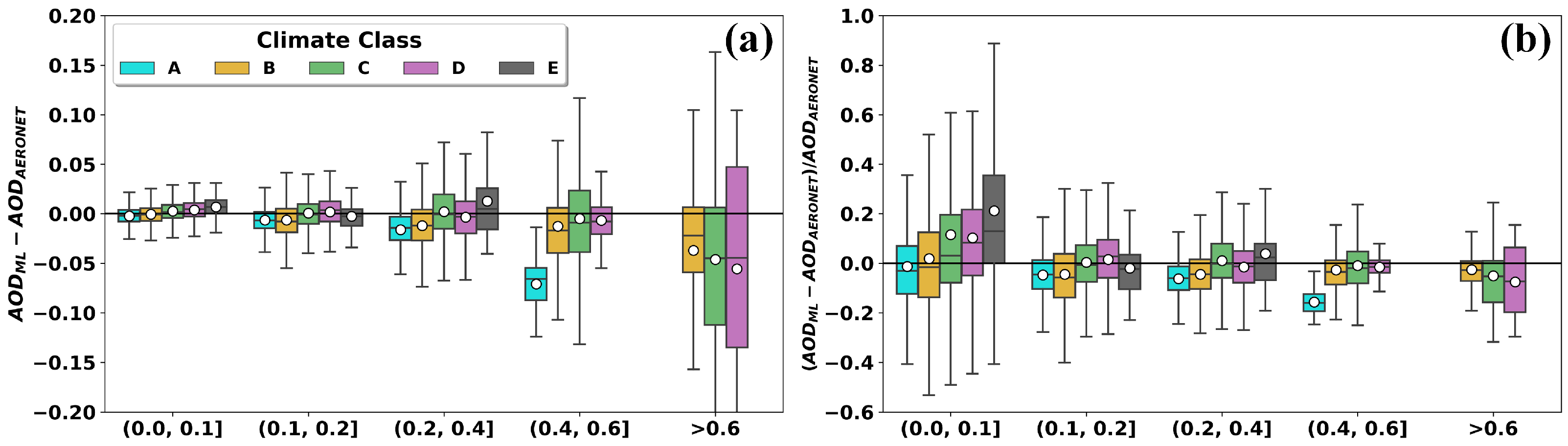
- The validation process includes comparisons against AERONET measurement locations with diverse climatic and aerosol characteristics.
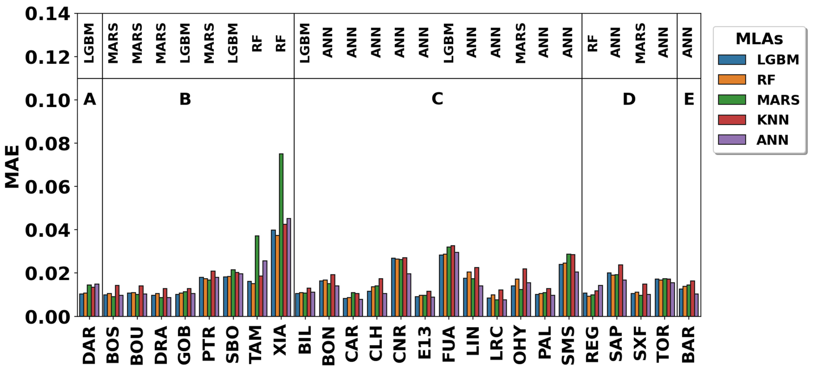
- MLAs with different prediction mechanisms are benchmarked to identify the “optimal” approach for retrieving AOD.
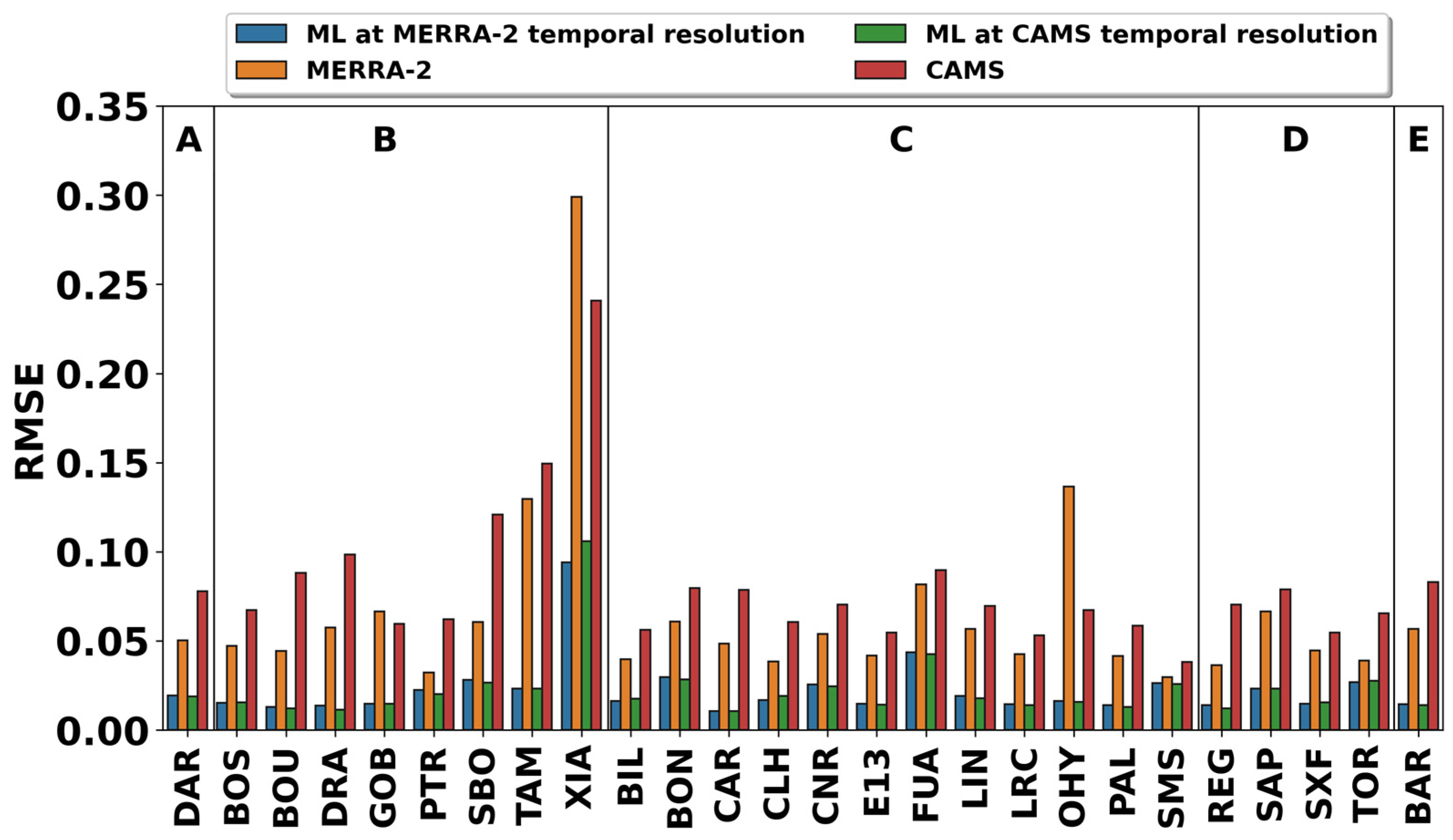
- The MLA-AOD retrievals are compared with AOD from reanalysis products (MERRA-2 and CAMSRA) through a comprehensive comparative analysis, showcasing the advantages of the proposed methodology at a regional level.
2. Datasets
2.1. Ground-Based Data
2.1.1. AERONET
2.1.2. BSRN
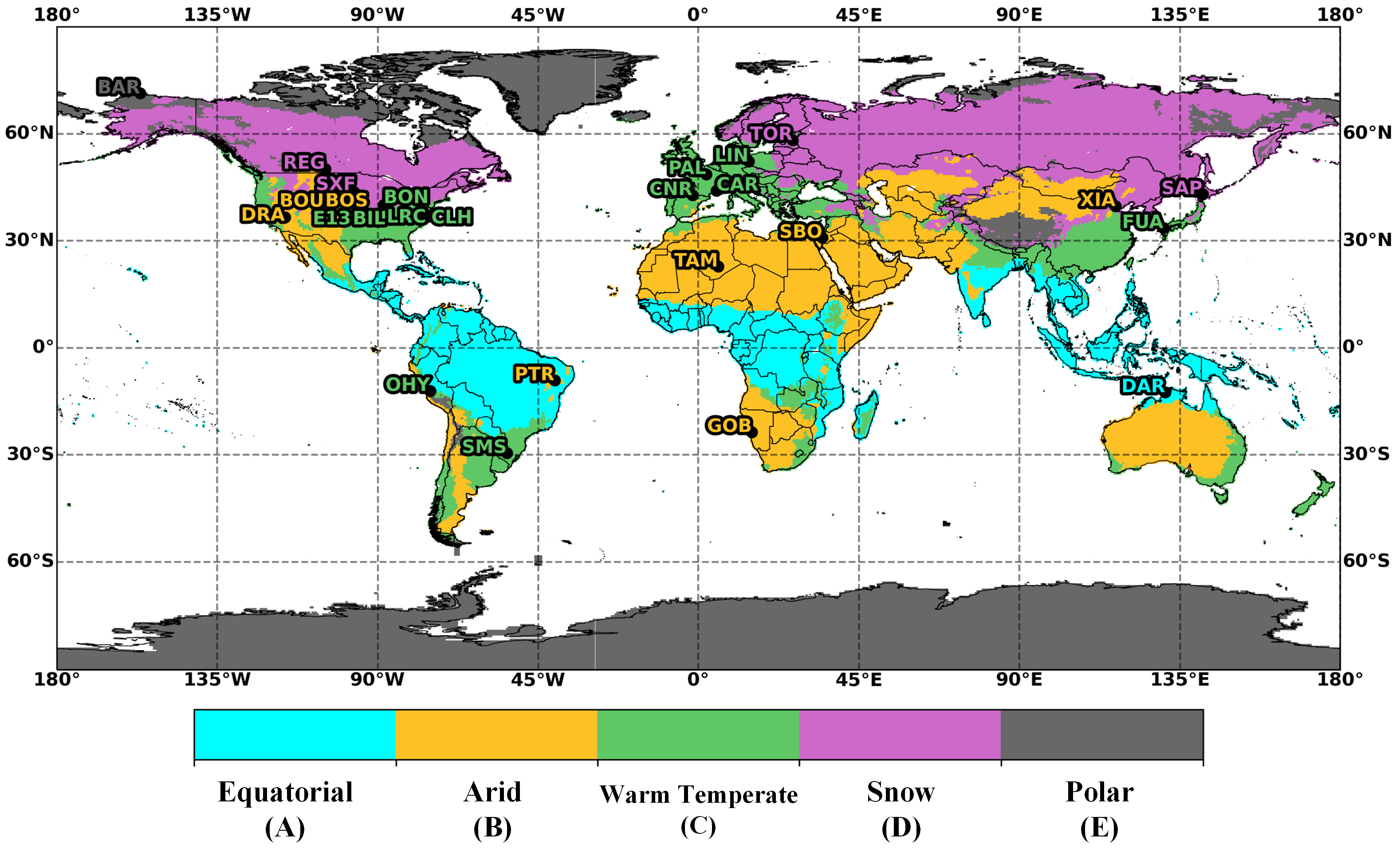
2.1.3. Stations’ Characteristics
2.2. Reanalysis Data
2.2.1. CAMSRA
2.2.2. MERRA-2
2.3. Satellite Data
MODIS
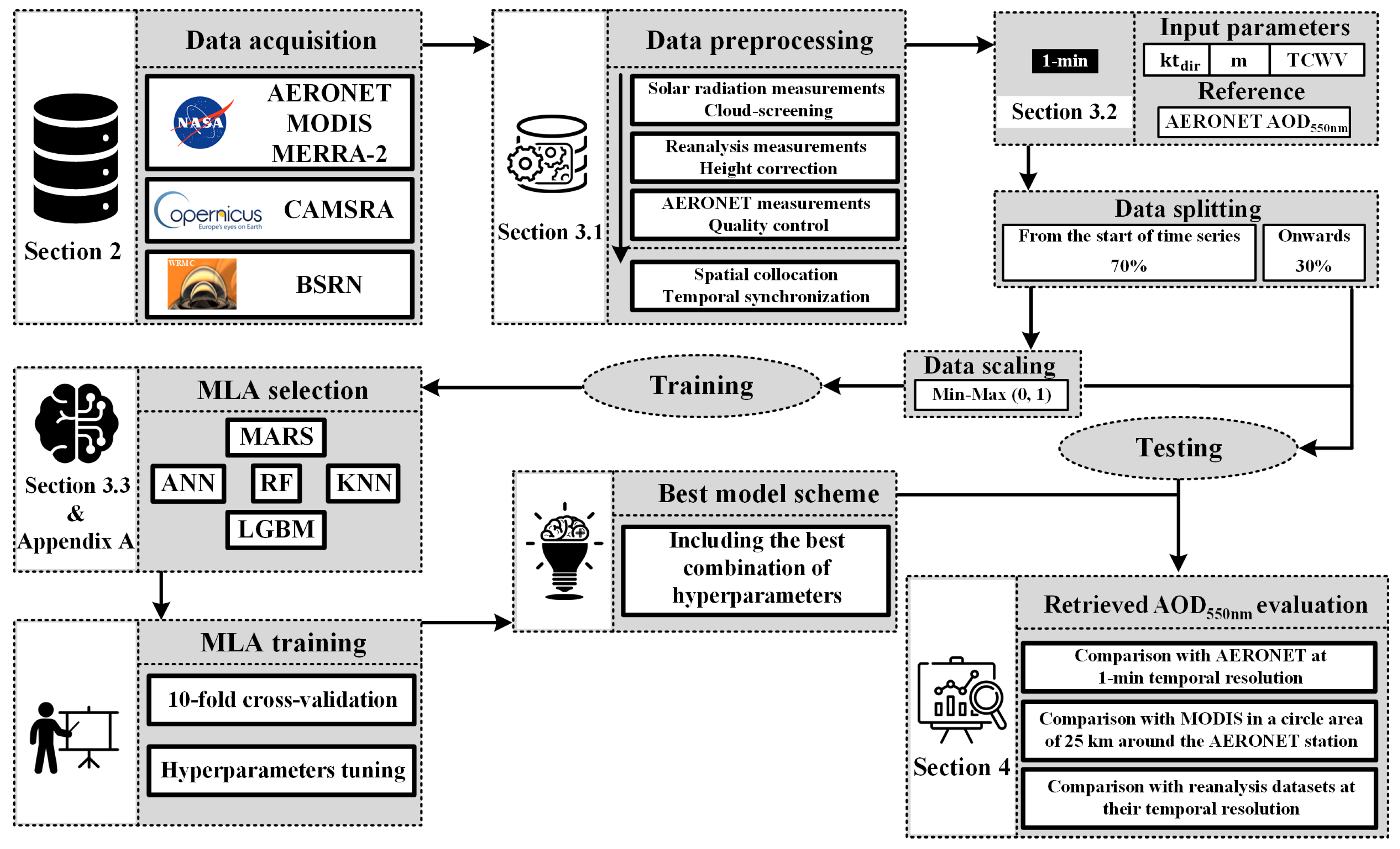
3. Methodology
3.1. Data Preprocessing
3.2. Input Parameters
3.3. Machine Learning Algorithms
4. Results
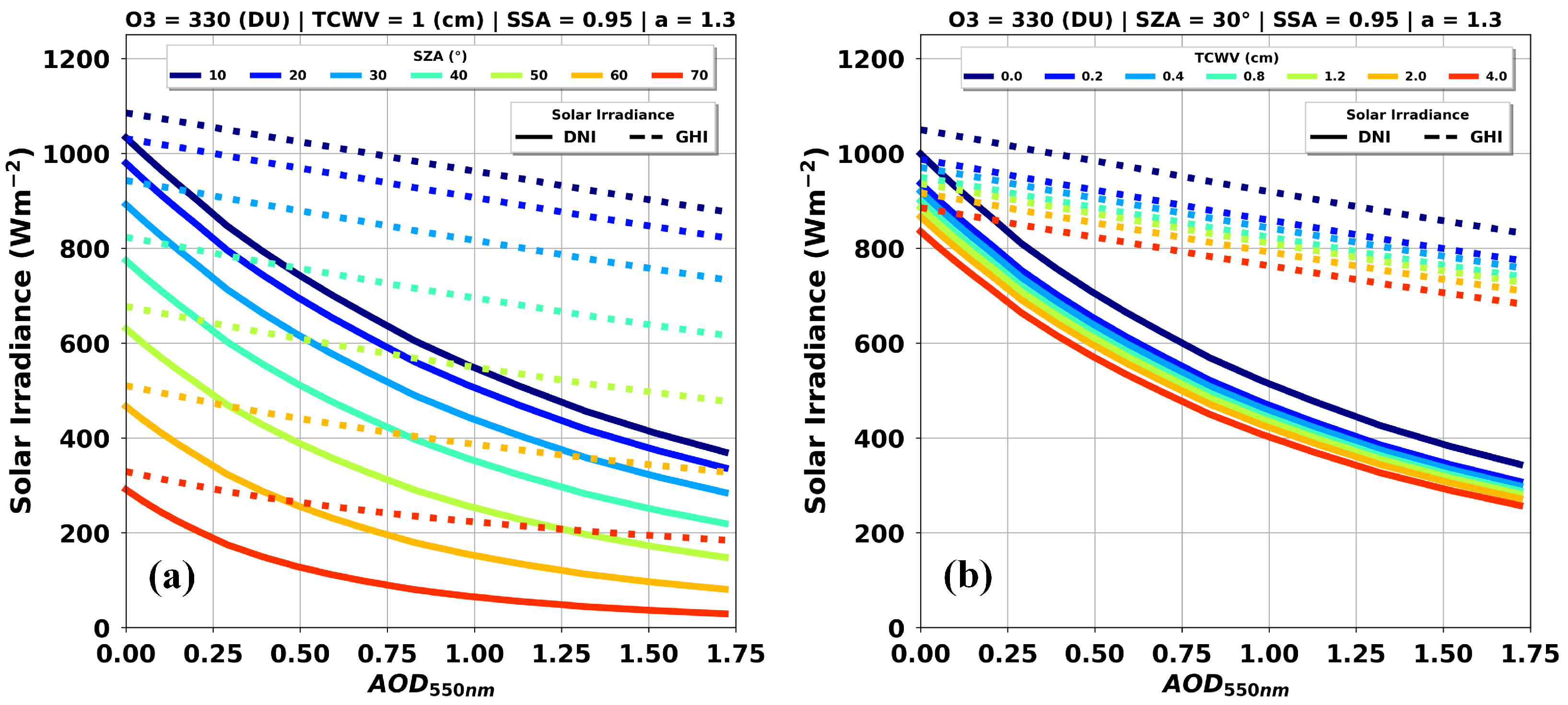
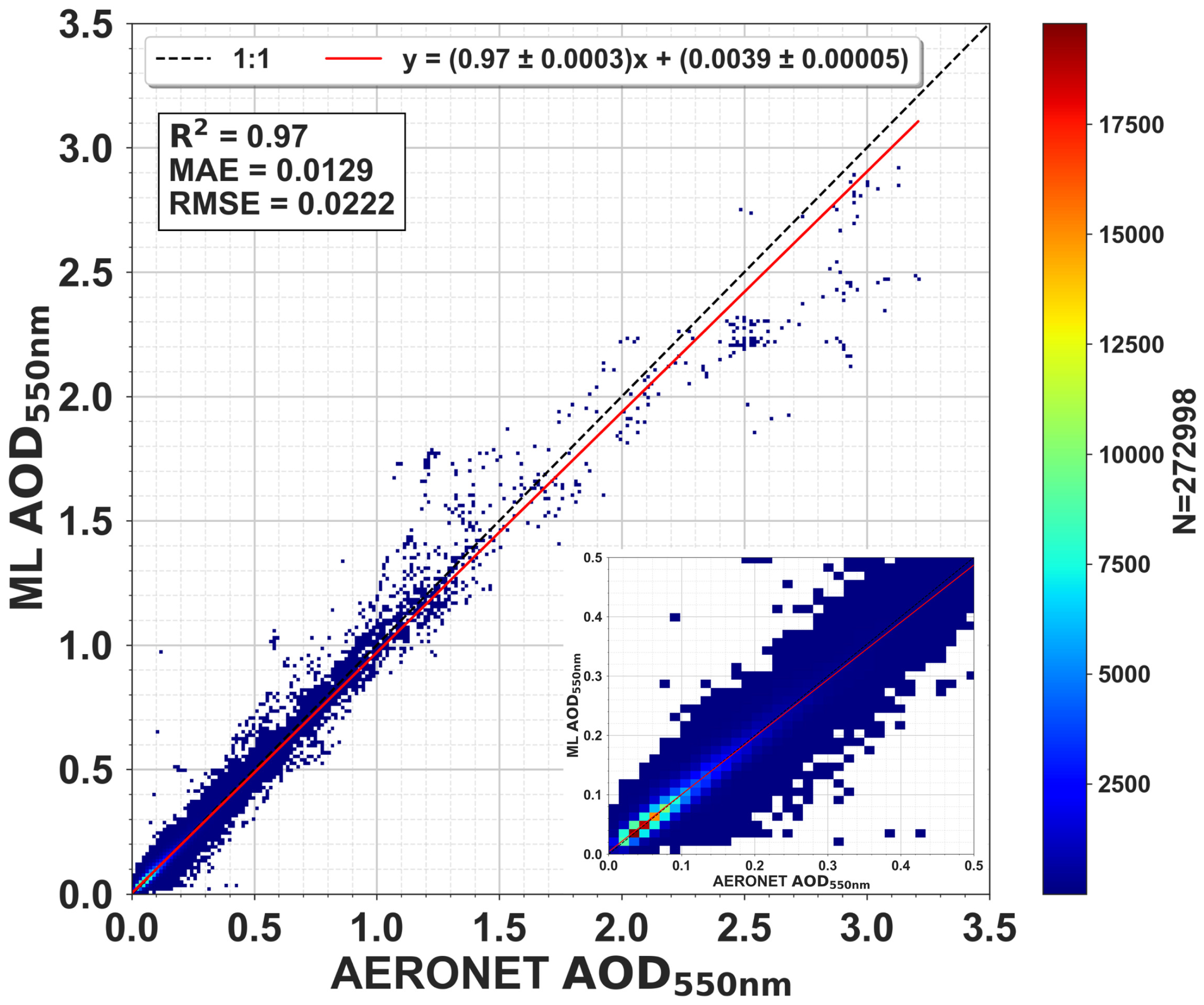
4.1. Direct Normal Irradiance vs. Global Horizontal Irradiance as Model Input
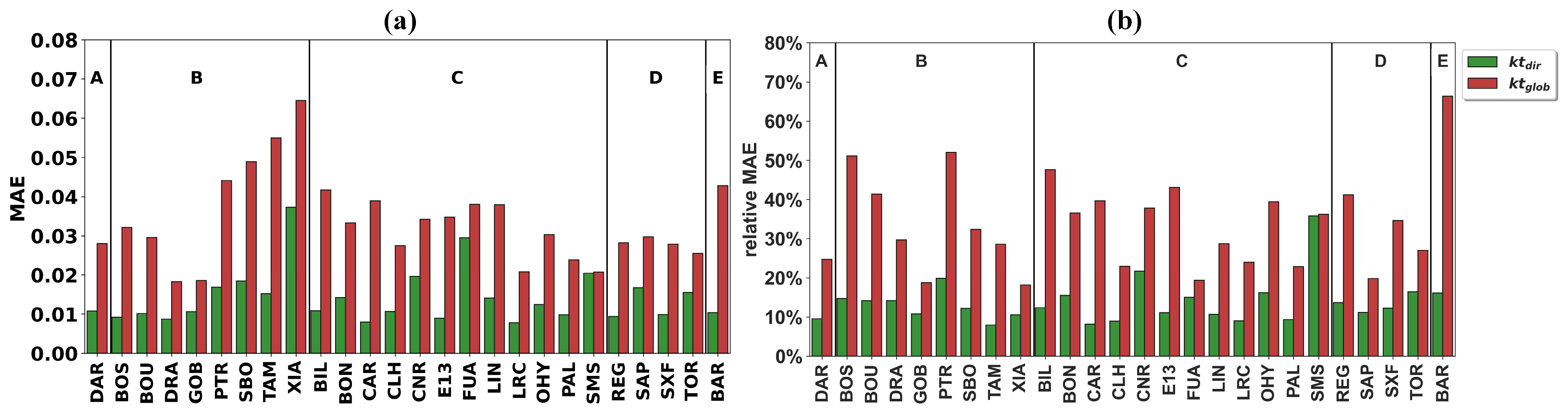
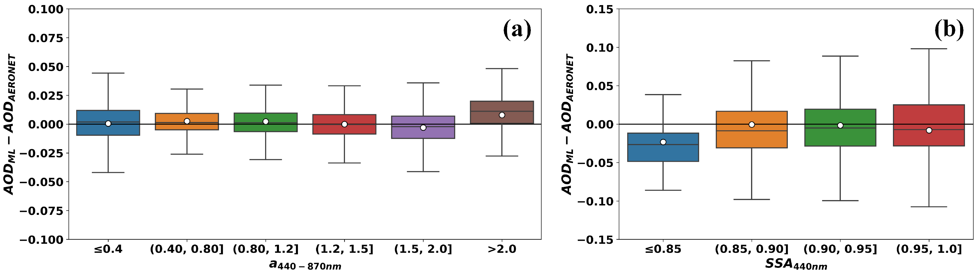
4.2. The Effect of Aerosol Properties on MLAs Retrieval Performance
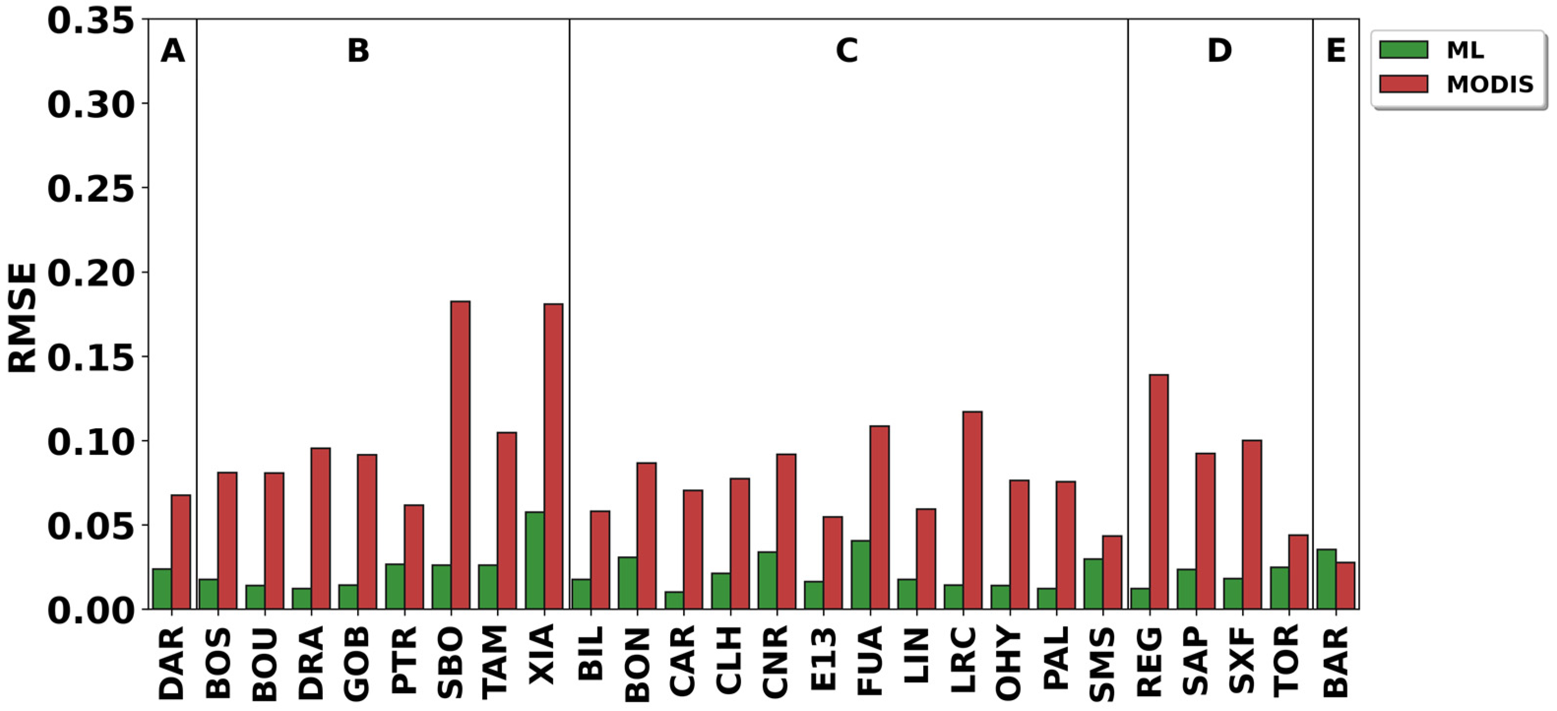
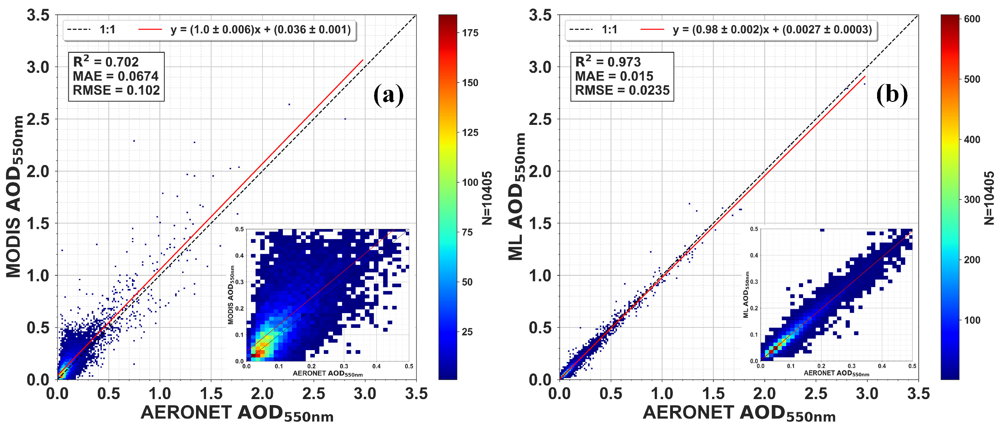
4.3. MLA-AOD vs. MODIS
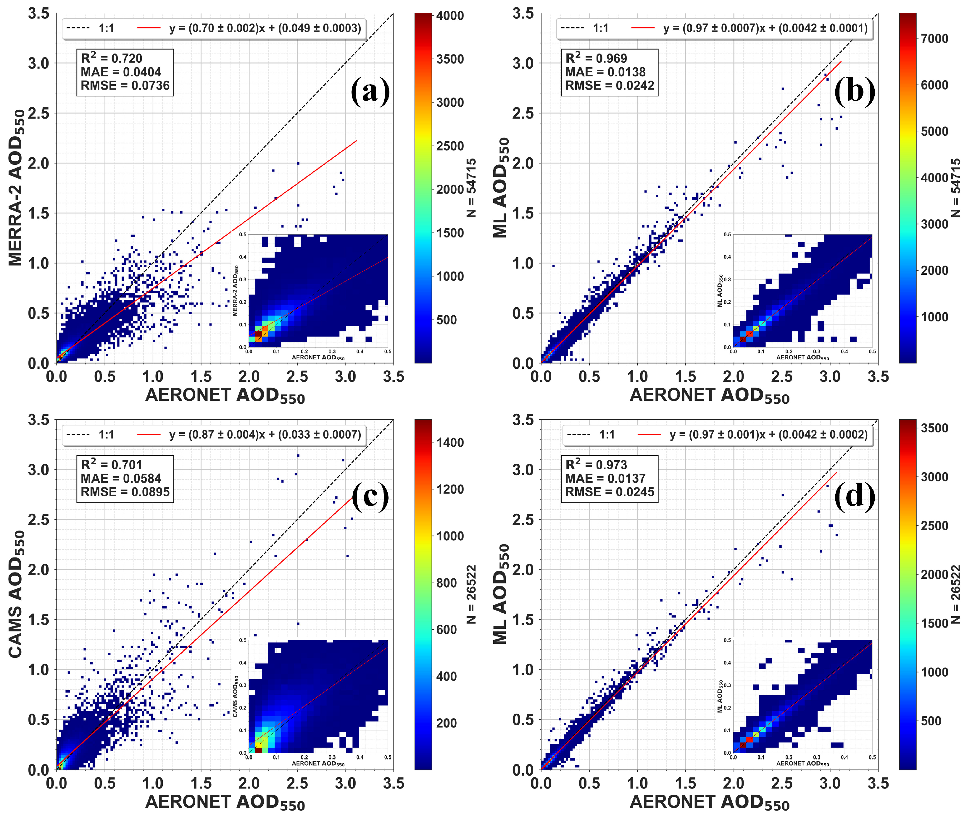
4.4. MLA-AOD vs. Reanalysis Products
5. Summary and Conclusions
Supplementary Materials
Author Contributions
Funding
Informed Consent Statement
Data Availability Statement
Acknowledgments
Conflicts of Interest
Appendix A
- Light Gradient Boosting Machine (LGBM)
- Random Forest (RF)
- Multivariate Adaptive Regression Splines (MARS)
- K-Nearest Neighbors (KNN)
- Artificial Neural Network (ANN)

| MLA | Package | Function |
|---|---|---|
| LGBM | LightGBM Python | lgb |
| RF | scikit–learn Python | RandomForestRegressor |
| MARS | py-earth Python | Earth |
| KNN | scikit–learn Python | KNeighborsRegressor |
| ANN | Keras Application Programming Interface | [83] |
References
- Gomis, M.I.; Huang, M.; Leitzell, K.; Lonnoy, E.; Matthews, J.B.R.; Maycock, T.K.; Waterfield, T.; Yelekçi, O.; Yu, R.; Zhou, B. IPCC, 2021: Climate Change 2021: The Physical Science Basis; Contribution of Working Group I to the Sixth Assessment Report of the Intergovernmental Panel on Climate Change; Cambridge University Press: Cambridge, UK; New York, NY, USA, 2021; in press. [Google Scholar] [CrossRef]
- Palacios-Peña, L.; Jiménez-Guerrero, P.; Baró, R.; Balzarini, A.; Bianconi, R.; Curci, G.; Landi, T.C.; Pirovano, G.; Prank, M.; Riccio, A.; et al. Aerosol optical properties over Europe: An evaluation of the AQMEII Phase 3 simulations against satellite observations. Atmos. Chem. Phys. 2019, 19, 2965–2990. [Google Scholar] [CrossRef]
- García, O.E.; Díaz, J.P.; Expósito, F.J.; Díaz, A.M.; Dubovik, O.; Derimian, Y.; Dubuisson, P.; Roger, J.-C. Shortwave radiative forcing and efficiency of key aerosol types using AERONET data. Atmos. Chem. Phys. 2012, 12, 5129–5145. [Google Scholar] [CrossRef]
- Gkikas, A.; Obiso, V.; Pérez García-Pando, C.; Jorba, O.; Hatzianastassiou, N.; Vendrell, L.; Basart, S.; Solomos, S.; Gassó, S.; Baldasano, J.M. Direct radiative effects during intense Mediterranean desert dust outbreaks. Atmos. Chem. Phys. 2018, 18, 8757–8787. [Google Scholar] [CrossRef]
- Korras-Carraca, M.-B.; Gkikas, A.; Matsoukas, C.; Hatzianastassiou, N. Global Clear-Sky Aerosol Speciated Direct Radiative Effects over 40 Years (1980–2019). Atmosphere 2021, 12, 1254. [Google Scholar] [CrossRef]
- Logothetis, S.-A.; Salamalikis, V.; Kazantzidis, A. The impact of different aerosol properties and types on direct aerosol radiative forcing and efficiency using AERONET version 3. Atmos. Res. 2021, 250, 105343. [Google Scholar] [CrossRef]
- Sengupta, M.; Xie, Y.; Lopez, A.; Habte, A.; Maclaurin, G.; Shelby, J. The National Solar Radiation Data Base (NSRDB). Renew. Sustain. Energy Rev. 2018, 89, 51–60. [Google Scholar] [CrossRef]
- Javadnia, E.; Abkar, A.; Schubert, P. Estimation of High-Resolution Surface Shortwave Radiative Fluxes Using SARA AOD over the Southern Great Plains. Remote Sens. 2017, 9, 1146. [Google Scholar] [CrossRef]
- Gueymard, C.A.; Habte, A.; Sengupta, M. Reducing Uncertainties in Large-Scale Solar Resource Data: The Impact of Aerosols. IEEE J. Photovolt. 2018, 8, 1732–1737. [Google Scholar] [CrossRef]
- Kosmopoulos, P.G.; Kazadzis, S.; Taylor, M.; Raptis, P.I.; Keramitsoglou, I.; Kiranoudis, C.; Bais, A.F. Assessment of surface solar irradiance derived from real-time modelling techniques and verification with ground-based measurements. Atmos. Meas. Tech. 2018, 11, 907–924. [Google Scholar] [CrossRef]
- Fountoukis, C.; Martín-Pomares, L.; Perez-Astudillo, D.; Bachour, D.; Gladich, I. Simulating global horizontal irradiance in the Arabian Peninsula: Sensitivity to explicit treatment of aerosols. Sol. Energy 2018, 163, 347–355. [Google Scholar] [CrossRef]
- Shi, H.; Li, W.; Fan, X.; Zhang, J.; Hu, B.; Husi, L.; Shang, H.; Han, X.; Song, Z.; Zhang, Y.; et al. First assessment of surface solar irradiance derived from Himawari-8 across China. Sol. Energy 2018, 174, 164–170. [Google Scholar] [CrossRef]
- Zhang, Y.; He, T.; Liang, S.; Wang, D.; Yu, Y. Estimation of all-sky instantaneous surface incident shortwave radiation from Moderate Resolution Imaging Spectroradiometer data using optimization method. Remote Sens. Environ. 2018, 209, 468–479. [Google Scholar] [CrossRef]
- Vamvakas, I.; Salamalikis, V.; Benitez, D.; Al-Salaymeh, A.; Bouaichaoui, S.; Yassaa, N.; Guizani, A.; Kazantzidis, A. Estimation of global horizontal irradiance using satellite-derived data across Middle East-North Africa: The role of aerosol optical properties and site-adaptation methodologies. Renew. Energy 2020, 157, 312–331. [Google Scholar] [CrossRef]
- Polo, J.; Fernández-Peruchena, C.; Salamalikis, V.; Mazorra-Aguiar, L.; Turpin, M.; Martín-Pomares, L.; Kazantzidis, A.; Blanc, P.; Remund, J. Benchmarking on improvement and site-adaptation techniques for modeled solar radiation datasets. Sol. Energy 2020, 201, 469–479. [Google Scholar] [CrossRef]
- Salamalikis, V.; Vamvakas, I.; Blanc, P.; Kazantzidis, A. Ground-based validation of aerosol optical depth from CAMS reanalysis project: An uncertainty input on direct normal irradiance under cloud-free conditions. Renew. Energy 2021, 170, 847–857. [Google Scholar] [CrossRef]
- Fountoulakis, I.; Kosmopoulos, P.; Papachristopoulou, K.; Raptis, I.-P.; Mamouri, R.-E.; Nisantzi, A.; Gkikas, A.; Witthuhn, J.; Bley, S.; Moustaka, A.; et al. Effects of Aerosols and Clouds on the Levels of Surface Solar Radiation and Solar Energy in Cyprus. Remote Sens. 2021, 13, 2319. [Google Scholar] [CrossRef]
- Holben, B.N.; Eck, T.F.; Slutsker, I.; Tanré, D.; Buis, J.P.; Setzer, A.; Vermote, E.; Reagan, J.A.; Kaufman, Y.J.; Nakajima, T.; et al. AERONET—A Federated Instrument Network and Data Archive for Aerosol Characterization. Remote Sens. Environ. 1998, 66, 1–16. [Google Scholar] [CrossRef]
- Zender, C.S.; Miller, R.; Tegen, I. Quantifying mineral dust mass budgets: Terminology, constraints, and current estimates. Eos Trans. Am. Geophys. Union 2004, 85, 509–512. [Google Scholar] [CrossRef]
- Textor, C.; Schulz, M.; Guibert, S.; Kinne, S.; Balkanski, Y.; Bauer, S.; Berntsen, T.; Berglen, T.; Boucher, O.; Chin, M.; et al. Analysis and quantification of the diversities of aerosol life cycles within AeroCom. Atmos. Chem. Phys. 2006, 6, 1777–1813. [Google Scholar] [CrossRef]
- Kok, J.F.; Ridley, D.A.; Zhou, Q.; Miller, R.L.; Zhao, C.; Heald, C.L.; Ward, D.S.; Albani, S.; Haustein, K. Smaller desert dust cooling effect estimated from analysis of dust size and abundance. Nat. Geosci. 2017, 10, 274–278. [Google Scholar] [CrossRef]
- Wei, X.; Chang, N.-B.; Bai, K.; Gao, W. Satellite remote sensing of aerosol optical depth: Advances, challenges, and perspectives. Crit. Rev. Environ. Sci. Technol. 2019, 50, 1640–1725. [Google Scholar] [CrossRef]
- Paciorek, C.J.; Liu, Y.; Moreno-Macias, H.; Kondragunta, S. Spatio-temporal associations between GOES aerosol optical depth retrievals and ground-level PM2.5. Environ. Sci. Technol. 2008, 42, 5800–5806. [Google Scholar] [CrossRef] [PubMed]
- Lindfors, A.V.; Kouremeti, N.; Arola, A.; Kazadzis, S.; Bais, A.F.; Laaksonen, A. Effective aerosol optical depth from pyranometer measurements of surface solar radiation (global radiation) at Thessaloniki, Greece. Atmos. Chem. Phys. 2013, 13, 3733–3741. [Google Scholar] [CrossRef]
- Salmon, A.; Quiñones, G.; Soto, G.; Polo, J.; Gueymard, C.; Ibarra, M.; Cardemil, J.; Escobar, R.; Marzo, A. Advances in aerosol optical depth evaluation from broadband direct normal irradiance measurements. Sol. Energy 2021, 221, 206–217. [Google Scholar] [CrossRef]
- Seo, J.; Choi, H.; Oh, Y. Potential of AOD Retrieval Using Atmospheric Emitted Radiance Interferometer (AERI). Remote Sens. 2022, 14, 407. [Google Scholar] [CrossRef]
- Herrero-Anta, S.; Román, R.; Mateos, D.; González, R.; Antuña-Sánchez, J.C.; Herreras-Giralda, M.; Almansa, A.F.; González-Fernández, D.; Herrero del Barrio, C.; Toledano, C.; et al. Retrieval of aerosol properties from zenith sky radiance measurements. Atmos. Meas. Tech. 2023, 16, 4423–4443. [Google Scholar] [CrossRef]
- Li, J.; Liu, R.; Liu, S.C.; Shiu, C.J.; Wang, J.; Zhang, Y. Trends in aerosol optical depth in northern China retrieved from sunshine duration data. Geophys. Res. Lett. 2016, 43, 431–439. [Google Scholar] [CrossRef]
- Sanchez-Romero, A.; Sanchez-Lorenzo, A.; González, J.A.; Calbó, J. Reconstruction of long-term aerosol optical depth series with sunshine duration records. Geophys. Res. Lett. 2016, 43, 1296–1305. [Google Scholar] [CrossRef]
- Wandji Nyamsi, W.; Lipponen, A.; Sanchez-Lorenzo, A.; Wild, M.; Arola, A. A hybrid method for reconstructing the historical evolution of aerosol optical depth from sunshine duration measurements. Atmos. Meas. Tech. 2020, 13, 3061–3079. [Google Scholar] [CrossRef]
- Kazantzidis, A.; Tzoumanikas, P.; Nikitidou, E.; Salamalikis, V.; Wilbert, S.; Prahl, C. Application of Simple All-sky Imagers for the Estimation of Aerosol Optical Depth. AIP Conf. Proc. 2017, 1850, 140012. [Google Scholar] [CrossRef]
- Román, R.; Antuña-Sánchez, J.C.; Cachorro, V.E.; Toledano, C.; Torres, B.; Mateos, D.; Fuertes, D.; López, C.; González, R.; Lapionok, T.; et al. Retrieval of aerosol properties using relative radiance measurements from an all-sky camera. Atmos. Meas. Tech. 2022, 15, 407–433. [Google Scholar] [CrossRef]
- Scarlatti, F.; Gómez-Amo, J.L.; Valdelomar, P.C.; Estellés, V.; Utrillas, M.P. A Machine Learning Approach to Derive Aerosol Properties from All-Sky Camera Imagery. Remote Sens. 2023, 15, 1676. [Google Scholar] [CrossRef]
- Logothetis, S.-A.; Giannaklis, C.-P.; Salamalikis, V.; Tzoumanikas, P.; Raptis, P.-I.; Amiridis, V.; Eleftheratos, K.; Kazantzidis, A. Aerosol Optical Properties and Type Retrieval via Machine Learning and an All-Sky Imager. Atmosphere 2023, 14, 1266. [Google Scholar] [CrossRef]
- Olcese, L.E.; Palancar, G.G.; Toselli, B.M. A method to estimate missing AERONET AOD values based on artificial neural networks. Atmos. Environ. 2015, 113, 140–150. [Google Scholar] [CrossRef]
- Huttunen, J.; Kokkola, H.; Mielonen, T.; Mononen, M.E.J.; Lipponen, A.; Reunanen, J.; Lindfors, A.V.; Mikkonen, S.; Lehtinen, K.E.J.; Kouremeti, N.; et al. Retrieval of aerosol optical depth from surface solar radiation measurements using machine learning algorithms, non-linear regression and a radiative transfer-based look-up table. Atmos. Chem. Phys. 2016, 16, 8181–8191. [Google Scholar] [CrossRef]
- Nabavi, S.O.; Haimberger, L.; Abbasi, R.; Samimi, C. Prediction of aerosol optical depth in West Asia using deterministic models and machine learning algorithms. Aeolian Res. 2018, 35, 69–84. [Google Scholar] [CrossRef]
- Kolios, S.; Hatzianastassiou, N. Quantitative Aerosol Optical Depth Detection during Dust Outbreaks from Meteosat Imagery Using an Artificial Neural Network Model. Remote Sens. 2019, 11, 1022. [Google Scholar] [CrossRef]
- Zbizika, R.; Pakszys, P.; Zielinski, T. Deep Neural Networks for Aerosol Optical Depth Retrieval. Atmosphere 2022, 13, 101. [Google Scholar] [CrossRef]
- Dubovik, O.; Lapyonok, T.; Litvinov, P.; Herman, M.; Fuertes, D.; Ducos, F.; Lopatin, A.; Chaikovsky, A.; Torres, B.; Derimian, Y.; et al. GRASP: A versatile algorithm for characterizing the atmosphere. SPIE Newsroom 2014, 25, 2-1201408. [Google Scholar] [CrossRef]
- Dubovik, O.; King, M.D. A flexible inversion algorithm for retrieval of aerosol optical properties from sun and sky radiance measurements. J. Geophys. Res. 2000, 105, 20673–20696. [Google Scholar] [CrossRef]
- Giles, D.M.; Sinyuk, A.; Sorokin, M.G.; Schafer, J.S.; Smirnov, A.; Slutsker, I.; Eck, T.F.; Holben, B.N.; Lewis, J.R.; Campbell, J.R.; et al. Advancements in the Aerosol Robotic Network (AERONET) Version 3 database—Automated near-real-time quality control algorithm with improved cloud screening for Sun photometer aerosol optical depth (AOD) measurements. Atmos. Meas. Tech. 2019, 12, 169–209. [Google Scholar] [CrossRef]
- Ohmura, A.; Gilgen, H.; Hegner, H.; Müller, G.; Wild, M.; Dutton, E.G.; Forgan, B.; Fröhlich, C.; Philipona, R.; Heimo, A.; et al. Baseline Surface Radiation Network (BSRN/WCRP): New Precision Radiometry for Climate Research. Bull. Am. Meteorol. Soc. 1998, 79, 2115–2136. [Google Scholar] [CrossRef]
- Driemel, A.; Augustine, J.; Behrens, K.; Colle, S.; Cox, C.; Cuevas-Agulló, E.; Denn, F.M.; Duprat, T.; Fukuda, M.; Grobe, H.; et al. Baseline Surface Radiation Network (BSRN): Structure and data description (1992–2017). Earth Syst. Sci. Data 2018, 10, 1491–1501. [Google Scholar] [CrossRef]
- Yang, D.; Yagli, G.M.; Quan, H. Quality Control for Solar Irradiance Data. In Proceedings of the 2018 IEEE Innovative Smart Grid Technologies—Asia (ISGT Asia), Singapore, 22–25 May 2018; pp. 208–213. [Google Scholar] [CrossRef]
- Yang, D. SolarData package update v1.1: R functions for easy access of Baseline Surface Radiation Network (BSRN). Sol. Energy 2019, 188, 970–975. [Google Scholar] [CrossRef]
- Kottek, M.; Grieser, J.; Beck, C.; Rudolf, B.; Rubel, F. World map of the Köppen-Geiger climate classification updated. Meteorol. Z. 2006, 15, 259–263. [Google Scholar] [CrossRef] [PubMed]
- Bryant, C.; Wheeler, N.R.; Rubel, F.; French, R.H. Kgc: Koeppen-Geiger Climatic Zones. R Package Version 1.0.0.2. 2017. Available online: https://cran.r-project.org/package=kgc (accessed on 22 March 2024).
- Bright, J.M.; Gueymard, C.A. Climate-specific and global validation of MODIS Aqua and Terra aerosol optical depth at 452 AERONET stations. Sol. Energy 2019, 183, 594–605. [Google Scholar] [CrossRef]
- Gueymard, C.A.; Yang, D. Worldwide validation of CAMS and MERRA-2 reanalysis aerosol optical depth products using 15 years of AERONET observations. Atmos. Environ. 2020, 225, 117216. [Google Scholar] [CrossRef]
- Wei, J.; Li, Z.; Peng, Y.; Sun, L. MODIS Collection 6.1 aerosol optical depth products over land and ocean: Validation and comparison. Atmos. Environ. 2019, 201, 428–440. [Google Scholar] [CrossRef]
- Inness, A.; Ades, M.; Agustí-Panareda, A.; Barré, J.; Benedictow, A.; Blechschmidt, A.-M.; Dominguez, J.J.; Engelen, R.; Eskes, H.; Flemming, J.; et al. The CAMS reanalysis of atmospheric composition. Atmos. Chem. Phys. 2019, 19, 3515–3556. [Google Scholar] [CrossRef]
- Popp, T.; de Leeuw, G.; Bingen, C.; Brühl, C.; Capelle, V.; Chedin, A.; Clarisse, L.; Dubovik, O.; Grainger, R.; Griesfeller, J.; et al. Development, production and evaluation of aerosol climate data records from european satellite observations (Aerosol_cci). Remote Sens. 2016, 8, 421. [Google Scholar] [CrossRef]
- Buchard, V.; Randles, C.A.; da Silva, A.M.; Darmenov, A.; Colarco, P.R.; Govindaraju, R.; Ferrare, R.; Hair, J.; Beyersdorf, A.J.; Ziemba, L.D.; et al. The MERRA-2 Aerosol Reanalysis, 1980 Onward. Part II: Evaluation and Case Studies. J. Clim. 2017, 30, 6851–6872. [Google Scholar] [CrossRef]
- Gelaro, R.; McCarty, W.; Suárez, M.J.; Todling, R.; Molod, A.; Takacs, L.; Randles, C.A.; Darmenov, A.; Bosilovich, M.G.; Reichle, R.; et al. The Modern-Era Retrospective Analysis for Research and Applications, Version 2 (MERRA-2). J. Clim. 2017, 30, 5419–5454. [Google Scholar] [CrossRef] [PubMed]
- Randles, C.A.; da Silva, A.M.; Buchard, V.; Colarco, P.R.; Darmenov, A.; Govindaraju, R.; Smirnov, A.; Holben, B.; Ferrare, R.; Hair, J.; et al. The MERRA-2 Aerosol Reanalysis, 1980 Onward. Part I: System Description and Data Assimilation Evaluation. J. Clim. 2017, 30, 6823–6850. [Google Scholar] [CrossRef] [PubMed]
- Levy, R.C.; Mattoo, S.; Munchak, L.A.; Remer, L.A.; Sayer, A.M.; Patadia, F.; Hsu, N.C. The Collection 6 MODIS aerosol products over land and ocean. Atmos. Meas. Tech. 2013, 6, 2989–3034. [Google Scholar] [CrossRef]
- Levy, R.C.; Remer, L.A.; Dubovik, O. Global aerosol optical properties and application to Moderate Resolution Imaging Spectroradiometer aerosol retrieval over land. J. Geophys. Res. Atmos. 2007, 112, D13210. [Google Scholar] [CrossRef]
- Levy, R.C.; Remer, L.A.; Mattoo, S.; Vermote, E.F.; Kaufman, Y.J. Second-generation operational algorithm: Retrieval of aerosol properties over land from inversion of Moderate Resolution Imaging Spectroradiometer spectral reflectance. J. Geophys. Res. Atmos. 2007, 112, D13211. [Google Scholar] [CrossRef]
- Levy, R.C.; Remer, L.A.; Kleidman, R.G.; Mattoo, S.; Ichoku, C.; Kahn, R.; Eck, T.F. Global evaluation of the Collection 5 MODIS dark-target aerosol products over land. Atmos. Chem. Phys. 2010, 10, 10399–10420. [Google Scholar] [CrossRef]
- Remer, L.A.; Tanre, D.; Kaufman, Y.J.; Ichoku, C.; Mattoo, S.; Levy, R.; Chu, D.A.; Holben, B.; Dubovik, O.; Smirnov, A.; et al. Validation of MODIS aerosol retrieval over ocean. Geophys. Res. Lett. 2002, 29, MOD3.1–MOD3.4. [Google Scholar] [CrossRef]
- Remer, L.A.; Kaufman, Y.J.; Tanre, D.; Mattoo, S.; Chu, D.A.; Martins, J.V.; Li, R.R.; Ichoku, C.; Levy, R.C.; Kleidman, R.G.; et al. The MODIS aerosol algorithm, products, and validation. J. Atmos. Sci. 2005, 62, 947–973. [Google Scholar] [CrossRef]
- Remer, L.A.; Kleidman, R.G.; Levy, R.C.; Kaufman, Y.J.; Tanré, D.; Mattoo, S.; Martins, J.V.; Ichoku, C.; Koren, I.; Yu, H.; et al. Global aerosol climatology from the MODIS satellite sensors. J. Geophys. Res. Atmos. 2008, 113, D14S07. [Google Scholar] [CrossRef]
- Sayer, A.M.; Hsu, N.C.; Bettenhausen, C.; Jeong, M.-J. Validation and uncertainty estimates for MODIS Collection 6 “Deep Blue” aerosol data. J. Geophys. Res. 2013, 118, 7864–7873. [Google Scholar] [CrossRef]
- Hsu, N.C.; Tsay, S.C.; King, M.D.; Herman, J.R. Aerosol Properties Over Bright-Reflecting Source Regions. IEEE Trans. Geosci. Remote 2004, 42, 557–569. [Google Scholar] [CrossRef]
- Reno, M.J.; Hansen, C.W. Identification of periods of clear sky irradiance in time series of GHI measurements. Renew. Energy 2016, 90, 520–531. [Google Scholar] [CrossRef]
- Kasten, F.; Young, A.T. Revised optical air mass tables and approximation formula. Appl. Opt. 1989, 28, 4735–4738. [Google Scholar] [CrossRef] [PubMed]
- Kaufman, Y.J.; Tanre, D.; Remer, L.; Vermote, E.; Chu, A.; Holben, B.N. Operational remote sensing of tropospheric aerosol over land from EOS moderate resolution imaging spectroradiometer. J. Geophys. Res. Atmos. 1997, 102, 17051–17067. [Google Scholar] [CrossRef]
- Mayer, B.; Kylling, A. Technical note: The libRadtran software package for radiative transfer calculations—Description and examples of use. Atmos. Chem. Phys. 2005, 5, 1855–1877. [Google Scholar] [CrossRef]
- Emde, C.; Buras-Schnell, R.; Kylling, A.; Mayer, B.; Gasteiger, J.; Hamann, U.; Kylling, J.; Richter, B.; Pause, C.; Dowling, T.; et al. The libRadtran software package for radiative transfer calculations (version 2.0.1). Geosci. Model Dev. 2016, 9, 1647–1672. [Google Scholar] [CrossRef]
- Ruiz-Arias, J.A.; Gueymard, C.A. Worldwide inter-comparison of clear-sky solar radiation models: Consensus-based review of direct and global irradiance components simulated at the earth surface. Sol. Energy 2018, 168, 10–29. [Google Scholar] [CrossRef]
- Ran, L.; Deng, Z.-Z.; Wang, P.C.; Xia, X.-A. Black carbon and wavelength-dependent aerosol absorption in the North China Plain based on two-year aethalometer measurements. Atmos. Environ. 2016, 142, 132–144. [Google Scholar] [CrossRef]
- Gueymard, C.A. Direct solar transmittance and irradiance predictions with broadband models. Part I: Detailed theoretical performance assessment. Sol. Energy 2003, 74, 355–379. [Google Scholar] [CrossRef]
- Guirado, C.; Cuevas, E.; Cachorro, V.E.; Toledano, C.; Alonso-Pérez, S.; Bustos, J.J.; Basart, S.; Romero, P.M.; Camino, C.; Mimouni, M.; et al. Aerosol characterization at the Saharan AERONET site Tamanrasset. Atmos. Chem. Phys. 2014, 14, 11753–11773. [Google Scholar] [CrossRef]
- Logothetis, S.-A.; Salamalikis, V.; Kazantzidis, A. Aerosol classification in Europe, Middle East, North Africa and Arabian Peninsula based on AERONET Version 3. Atmos. Res. 2020, 239, 104893. [Google Scholar] [CrossRef]
- Friedman, J.H. Greedy function approximation: A gradient boosting machine. Ann. Stat. 2001, 29, 1189–1232. [Google Scholar] [CrossRef]
- Ke, G.; Meng, Q.; Finley, T.; Wang, T.; Chen, W.; Ma, W.; Ye, Q.; Liu, T.-Y. LightGBM: A Highly Efficient Gradient Boosting Decision Tree, 9. Adv. Neural Inf. Process. Syst. 2017, 3147–3155. [Google Scholar] [CrossRef]
- Breiman, L. Random forests. Mach. Learn. 2001, 45, 5–32. [Google Scholar] [CrossRef]
- Friedman, J.H. Multivariate Adaptive Regression Splines. Ann. Stat. 1991, 19, 1–67. [Google Scholar] [CrossRef]
- Zhang, W.; Goh, A.T.C. Multivariate adaptive regression splines and neural network models for prediction of pile drivability. Geosci. Front. 2016, 7, 45–52. [Google Scholar] [CrossRef]
- Rosenblatt, F. The perceptron: A probabilistic model for information storage and organization in the brain. Psychol. Rev. 1958, 65, 386–408. [Google Scholar] [CrossRef]
- Kingma, D.P.; Ba, J. Adam: A Method for Stochastic Optimization. Available online: http://arxiv.org/abs/1412.6980 (accessed on 29 January 2017).
- Chollet, F. Keras. 2015. Available online: https://github.com/fchollet/keras (accessed on 22 March 2024).


Disclaimer/Publisher’s Note: The statements, opinions and data contained in all publications are solely those of the individual author(s) and contributor(s) and not of MDPI and/or the editor(s). MDPI and/or the editor(s) disclaim responsibility for any injury to people or property resulting from any ideas, methods, instructions or products referred to in the content. |
© 2024 by the authors. Licensee MDPI, Basel, Switzerland. This article is an open access article distributed under the terms and conditions of the Creative Commons Attribution (CC BY) license (https://creativecommons.org/licenses/by/4.0/).
Share and Cite
Logothetis, S.-A.; Salamalikis, V.; Kazantzidis, A. A Machine Learning Approach to Retrieving Aerosol Optical Depth Using Solar Radiation Measurements. Remote Sens. 2024, 16, 1132. https://doi.org/10.3390/rs16071132
Logothetis S-A, Salamalikis V, Kazantzidis A. A Machine Learning Approach to Retrieving Aerosol Optical Depth Using Solar Radiation Measurements. Remote Sensing. 2024; 16(7):1132. https://doi.org/10.3390/rs16071132
Chicago/Turabian StyleLogothetis, Stavros-Andreas, Vasileios Salamalikis, and Andreas Kazantzidis. 2024. "A Machine Learning Approach to Retrieving Aerosol Optical Depth Using Solar Radiation Measurements" Remote Sensing 16, no. 7: 1132. https://doi.org/10.3390/rs16071132
APA StyleLogothetis, S.-A., Salamalikis, V., & Kazantzidis, A. (2024). A Machine Learning Approach to Retrieving Aerosol Optical Depth Using Solar Radiation Measurements. Remote Sensing, 16(7), 1132. https://doi.org/10.3390/rs16071132