

A New Vegetation Observable Derived from Spaceborne GNSS-R and Its Application to Vegetation Water Content Retrieval


Abstract
1. Introduction
2. Data
2.1. CYGNSS
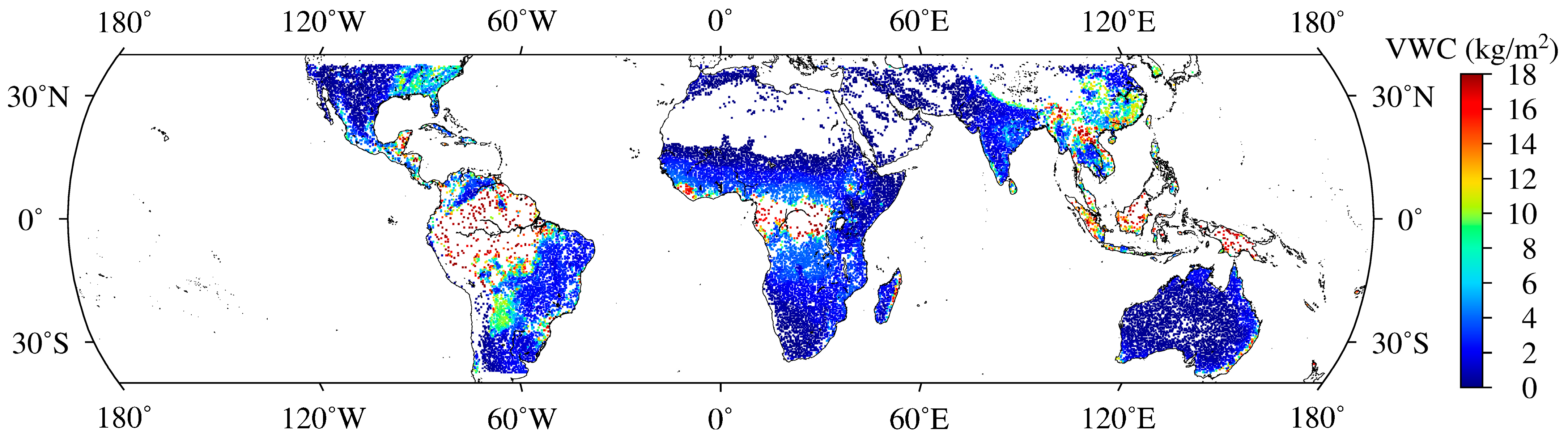
2.2. VWC
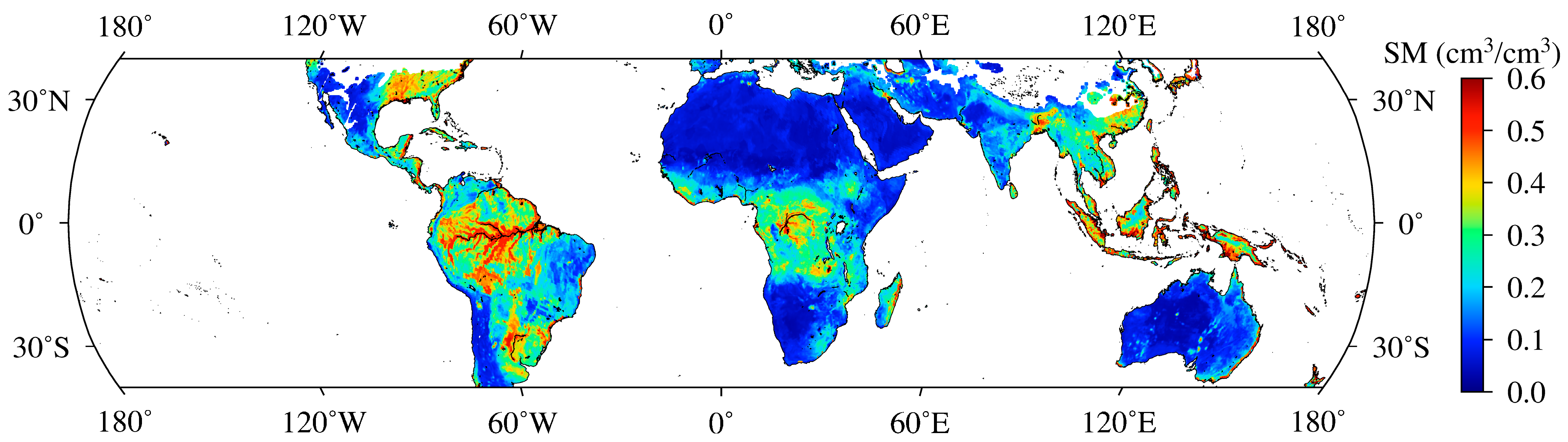
2.3. Soil Moisture
2.4. Land Cover
3. Derivation of the Vegetation Observables and the Correlation Analysis
3.1. Derivation of the Vegetation Observables from CYGNSS
3.2. Correlation Analysis Correlation Analysis between the GNSS-R Observables and Vegetation Parameters (VWC, AGB)
4. VWC Retrieval Models
4.1. Linear Model
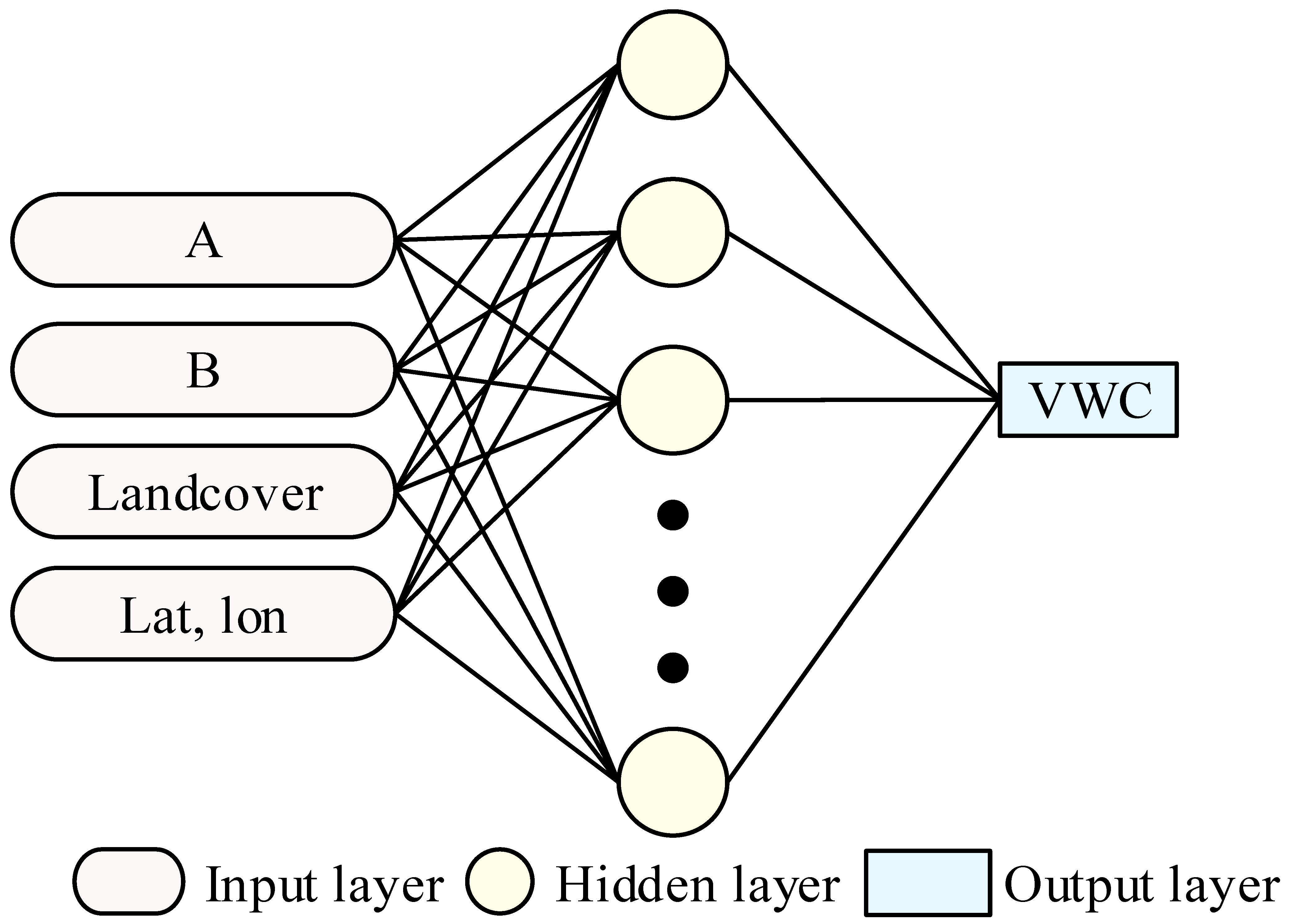
4.2. ANN Model
5. VWC Retrievals
6. Conclusions
Author Contributions
Funding
Data Availability Statement
Acknowledgments
Conflicts of Interest
References
- Kaplan, E.; Hegarty, C. Understanding GPS Principles and Applications, 2nd ed.; British Library Cataloguing in Publication Data; Artech House: Boston, MA, USA, 2006; pp. 1–723. [Google Scholar]
- Zhang, B.; Hou, P.; Zha, J.; Liu, T. PPP-RTK functional models formulated with undifferenced and uncombined GNSS observations. Satell. Navig. 2022, 3, 3. [Google Scholar] [CrossRef]
- Martin-Neira, M. A Pasive Reflectometry and Interferometry System (PARIS) Application to Ocean Altimetry. ESA J. 1993, 17, 331–355. [Google Scholar]
- Yu, K.; Li, Y.; Chang, X. Snow Depth Estimation Based on Combination of Pseudorange and Carrier Phase of GNSS Dual-Frequency Signals. IEEE Trans. Geosci. Remote. Sens. 2019, 57, 1817–1828. [Google Scholar] [CrossRef]
- Zhang, Z.; Guo, F.; Zhang, X. Triple-frequency Multi-GNSS reflectometry Snow Depth Retrieval by Using Clustering and Normalization Algorithm to Compensate Terrain variation. GPS Solut. 2020, 24, 52. [Google Scholar] [CrossRef]
- Wang, X.; He, X.; Xiao, R.; Song, M.; Jia, D. Millimeter to Centimeter Scale Precision Water-level Monitoring Using GNSS Reflectometry: Application to the South-to-North Water Diversion Project, China. Remote Sens. Environ. 2021, 265, 112645. [Google Scholar] [CrossRef]
- Wang, X.; He, X.; Zhang, Q. Evaluation and Combination of Quad-constellation Multi-GNSS Multipath Reflectometry Applied to Sea Level Retrieval. Remote Sens. Environ. 2019, 231, 111229. [Google Scholar] [CrossRef]
- Tabibia, S.; Geremia-Nievinskib, F.; Francisa, O.; van Dam, T. Tidal Analysis of GNSS Reflectometry Applied for Coastal Sea Level Sensing in Antarctica and Greenland. Remote Sens. Environ. 2020, 248, 111959. [Google Scholar] [CrossRef]
- Larson, K.M.; Small, E.E.; Gutmann, E.D.; Bilich, A.L.; Braun, J.J.; Zavorotny, V.U. Use of GPS Receivers as A Soil Moisture Network for Water Cycle Studies. Geophys. Res. Lett. 2008, 35, L24405. [Google Scholar] [CrossRef]
- Zhang, S.; Wang, T.; Wang, L.; Zhang, J.; Peng, J.; Liu, Q. Evaluation of GNSS-IR for Retrieving Soil Moisture and Vegetation Growth Characteristics in Wheat Farmland. J. Surv. Eng. 2021, 147, 4021009. [Google Scholar] [CrossRef]
- Li, Y.; Yu, K.; Li, J.; Jin, T.; Chang, X.; Zhang, Q.; Yang, S. Measuring Soil Moisture with Refracted GPS Signals. IEEE Geosci. Remote. Sens. Lett. 2022, 19, 2504205. [Google Scholar] [CrossRef]
- Alonsoarroyo, A.; Zavorotny, V.U.; Camps, A. Sea Ice Detection Using GNSS-R Data from UK TDS-1. In Proceedings of the 2016 IEEE International Geoscience and Remote Sensing Symposium (IGARSS), Beijing, China, 10–15 July 2016. [Google Scholar]
- Li, W.; Estel, C.; Fran, F.; Rius, A.; Ribó, S.; Martín-Neira, M. First Spaceborne Phase Altimetry Over Sea Ice Using TechDemoSat-1 GNSS-R Signals. Geophys. Res. Lett. 2017, 16, 8369–8376. [Google Scholar] [CrossRef]
- Cartwright, J.C.; Banks, J.; Srokosz, M. Sea Ice Detection Using GNSS-R Data from TechDemoSat-1. J. Geophys. Res. Ocean. 2019, 124, 5801–5810. [Google Scholar] [CrossRef]
- Zavorotnyand, V.U.; Voronovich, A.G. Scattering of GPS Signals from the Ocean with Wind Remote Sensing Application. IEEE Trans. Geosci. Remote Sens. 2000, 38, 951–964. [Google Scholar] [CrossRef]
- Clariziaand, M.P.; Ruf, C.S. Wind Speed Retrieval Algorithm for the Cyclone Global Navigation Satellite System (CYGNSS) Mission. IEEE T. Geosci. Remote 2016, 54, 4419–4432. [Google Scholar] [CrossRef]
- Asgarimehr, M.; Zhelavskaya, I.; Foti, G.; Reich, S.; Wickert, J. A GNSS-R Geophysical Model Function: Machine Learning for Wind Speed Retrievals. IEEE Geosci. Remote Sens. Lett. 2020, 17, 1333–1337. [Google Scholar] [CrossRef]
- Addabbo, P.; Di Bisceglie, M.; Galdi, C.; Giangregorio, G. An Algorithm for Wind Speed Retrieval from CYGNSS Space Observatories. In Proceedings of the 2018 IEEE International Geoscience and Remote Sensing Symposium (IGARSS), Valencia, Spain, 22–27 July 2018. [Google Scholar]
- Alonso-Arroyo, A.; Camps, A.; Park, H.; Pascual, D.; Onrubia, R.; Martín, F. Retrieval of Significant Wave Height and Mean Sea Surface Level Using the GNSS-R Interference Pattern Technique: Results from a Three-Month Field Campaign. IEEE Trans. Geosci. Remote Sens. 2015, 53, 3198–3209. [Google Scholar] [CrossRef]
- Wang, F.; Yang, D.K.; Li, W.Q.; Zhang, Y.Z. A New Retrieval Method of Significant Wave Height Based on Statistics of Scattered BeiDou GEO Signals. In Proceedings of the 28th International Technical Meeting of the Satellite Division of the Institute of Navigation (Ion Gnss+ 2015), Tampa, FL, USA, 14–18 September 2015. [Google Scholar]
- Yueh, S.H.; Shah, R.; Chaubell, M.J. A Semiempirical Modeling of Soil Moisture, Vegetation, and Surface Roughness Impact on CYGNSS Reflectometry Data. IEEE Trans. Geosci. Remote Sens. 2020, 60, 5800117. [Google Scholar] [CrossRef]
- Tyagi, S.; Pandey, D.K.; Putrevu, D. Sensitivity Analysis of CYGNSS Derived Radar Reflectivity for Soil Moisture Retrieval over India: Initial results. In Proceedings of the 2019 IEEE 16th India Council International Conference (INDICON), Rajkot, India, 13–15 December 2019. [Google Scholar]
- Chew, C.; Shah, R.; Zuffada, C.; Hajj, G.; Masters, D.; Mannucci, A.J. Demonstrating Soil Moisture Remote Sensing with Observations from the UK TechDemoSat-1 Satellite Mission. Geophys. Res. Lett. 2016, 43, 3317–3324. [Google Scholar] [CrossRef]
- Yan, Q.; Huang, W.; Jin, S.; Jia, Y. Pan-tropical Soil Moisture Mapping Based on A Three-layer Model from CYGNSS GNSS-R Data. Remote Sens. Environ. 2020, 247, 111944. [Google Scholar] [CrossRef]
- Morris, M.; Chew, C.; Reager, J.T.; Shah, R.; Zuffada, C. A Novel Approach to Monitoring Wetland Dynamics Using CYGNSS: Everglades Case Study. Remote Sens. Environ. 2019, 233, 111417. [Google Scholar] [CrossRef]
- Nghiem, S.V.; Zuffada, C.; Shah, R.; Chew, C.; Lowe, S.T.; Mannucci, A.J.; Cardellach, E.; Brakenridge, G.R.; Geller, G.; Rosenqvist, A. Wetland Monitoring with Global Navigation Satellite System Reflectometry. Earth Space Sci. 2017, 4, 16–39. [Google Scholar] [CrossRef] [PubMed]
- Unnithan, S.L.K.; Biswal, B.; Rudiger, C. Flood Inundation Mapping by Combining GNSS-R Signals with Topographical Information. Remote Sens. 2020, 12, 3026. [Google Scholar] [CrossRef]
- Loria, E.; O’Brien, A.; Zavorotny, V.; Downs, B.; Zuffada, C. Analysis of Scattering Characteristics from Inland Bodies of Water Observed by CYGNSS. Remote Sens. Environ. 2020, 245, 111825. [Google Scholar] [CrossRef]
- Stilla, D.; Zribi, M.; Pierdicca, N.; Baghdadi, N.; Huc, M. Desert Roughness Retrieval Using CYGNSS GNSS-R Data. Remote Sens. 2020, 12, 743. [Google Scholar] [CrossRef]
- Carreno-Luengo, H.; Ruf, C.S. Retrieving Freeze/thaw Surface State from CYGNSS Measurements. IEEE Trans. Geosci. Remote Sens. 2021, 60, 4302313. [Google Scholar] [CrossRef]
- Carreno-Luengo, H.; Lowe, S.; Zuffada, C.; Esterhuizen, S.; Oveisgharan, S. Spaceborne GNSS-R from the SMAP Mission: First Assessment of Polarimetric Scatterometry over Land and Cryosphere. Remote Sens. 2017, 9, 362. [Google Scholar] [CrossRef]
- Carreno-Luengo, H.; Luzi, G.; Crosetto, M. Above-Ground Biomass Retrieval over Tropical Forests: A Novel GNSS-R Approach with CYGNSS. Remote Sens. 2020, 12, 1368. [Google Scholar] [CrossRef]
- Chen, F.; Guo, F.; Liu, L.; Nan, Y. An Improved Method for Pan-Tropical Above-Ground Biomass and Canopy Height Retrieval Using CYGNSS. Remote Sens. 2021, 13, 2491. [Google Scholar] [CrossRef]
- Camps, A.; Park, H.; Pablos, M.; Foti, G.; Gommenginger, C.P.; Liu, P.-W.; Judge, J. Sensitivity of GNSS-R Spaceborne Observations to Soil Moisture and Vegetation. IEEE J.-STARS 2016, 9, 4730–4742. [Google Scholar] [CrossRef]
- Carreno-Luengo, H.; Luzi, G.; Crosetto, M. Sensitivity of CYGNSS Bistatic Reflectivity and SMAP Microwave Radiometry Brightness Temperature to Geophysical Parameters over Land Surfaces. IEEE J.-STARS 2018, 12, 107–122. [Google Scholar] [CrossRef]
- Chan, S.; Bindlish, R.; Hunt, R.; Jackson, T.; Kimball, J. Ancillary Data Report: Vegetation Water Content. SMAP Proj. Doc., JPL D-53061. SMAP Data Documents. 2013. Available online: https://smap.jpl.nasa.gov/system/internal_resources/details/original/289_047_veg_water.pdf (accessed on 1 August 2022).
- Zheng, X.; Ding, Y.; Zhao, X.; Yu, B.; Xiaofeng, L.; Kai, Z.; Tao, J. Uncertainty Evaluation at Three Spatial Scales for the NDVI-based VWC Estimation Method Used in the SMAP Algorithm. Remote Sens. Lett. 2019, 10, 563–572. [Google Scholar]
- Camps, A.; Park, H.; Bandeiras, J.; Barbosa, J.; Sousa, A.; d’Addio, S.; Martin-Neira, M. Microwave Imaging Radiometers by Aperture Synthesis—Performance Simulator (Part 1): Radiative Transfer Module. J. Imaging 2016, 2, 17. [Google Scholar] [CrossRef]
- Tsang, L.; Kong, J.A.; Shin, R.T. Theory of Microwave Remote Sensing; Wiley: New York, NY, USA, 1985. [Google Scholar]
- Konings, A.G.; Piles, M.; Rötzer, K.; McColl, K.A.; Chan, S.K.; Entekhabi, D. Vegetation Optical Depth and Scattering Albedo Retrieval Using Time Series of Dual-polarized L-band Radiometer Observations. Remote Sens. Environ. 2016, 172, 178–189. [Google Scholar] [CrossRef]
- Konings, A.G.; Saatchi, S.S.; Frankenberg, C.; Keller, M.; Leshyk, V.; Anderegg, W.R.; Humphrey, V.; Matheny, A.M.; Trugman, A.; Sack, L.; et al. Detecting Forest Response to Droughts with Global Observations of Vegetation Water Content. Glob. Chang. Biol. 2021, 27, 6005–6024. [Google Scholar] [CrossRef]


| Month | A | B | ||||
|---|---|---|---|---|---|---|
| VWC | AGB | VWC | AGB | VWC | AGB | |
| 1 | 0.104 | 0.113 | 0.619 | 0.355 | −0.210 | −0.094 |
| 2 | 0.086 | 0.065 | 0.618 | 0.397 | −0.218 | −0.094 |
| 3 | 0.040 | 0.159 | 0.642 | 0.388 | −0.230 | 0.093 |
| 4 | 0.119 | 0.082 | 0.648 | 0.389 | −0.230 | −0.121 |
| 5 | 0.156 | −0.028 | 0.631 | 0.342 | −0.238 | −0.158 |
| 6 | 0.144 | 0.028 | 0.640 | 0.270 | −0.224 | −0.170 |
| 7 | 0.131 | −0.027 | 0.651 | 0.435 | −0.191 | −0.183 |
| 8 | 0.012 | −0.064 | 0.662 | 0.497 | −0.268 | −0.261 |
| 9 | 0.088 | 0.021 | 0.684 | 0.523 | −0.259 | −0.252 |
| 10 | 0.024 | −0.033 | 0.692 | 0.589 | −0.285 | −0.273 |
| 11 | 0.066 | −0.031 | 0.690 | 0.548 | −0.302 | −0.275 |
| 12 | 0.069 | −0.031 | 0.678 | 0.548 | −0.323 | −0.279 |
| 1–6 | 0.242 | 0.101 | 0.607 | 0.390 | −0.223 | −0.137 |
| 7–12 | −0.029 | −0.210 | 0.742 | 0.624 | −0.317 | −0.298 |
| Model | Input Features |
|---|---|
| Model 1 | B |
| Model 2 | B, A |
| Model 3 | B, A, landcover |
| Model 4 | B, A, lat, lon |
| Model 5 | B, A, landcover, lat, lon |
| Model | MAE | MRAE | RMSE | Correlation Coefficient | Samples |
|---|---|---|---|---|---|
| Linear Model 1/Equation (16) | 1.759 | 0.644 | 2.751 | 0.741 | 32304 |
| ANN Model 1 | 1.623 | 0.593 | 2.506 | 0.773 | 34225 |
| Linear Model 2/Equation (17) | 1.818 | 0.664 | 2.684 | 0.747 | 32304 |
| ANN Model 2 | 1.481 | 0.542 | 2.439 | 0.787 | 34225 |
| Linear Model 3/Equation (18) | 1.662 | 0.547 | 2.327 | 0.790 | 32304 |
| ANN Model 3 | 0.836 | 0.244 | 1.507 | 0.931 | 34225 |
| Linear Model 4/Equation (19) | 1.609 | 0.587 | 2.641 | 0.763 | 32304 |
| ANN Model 4 | 0.962 | 0.287 | 1.496 | 0.932 | 34225 |
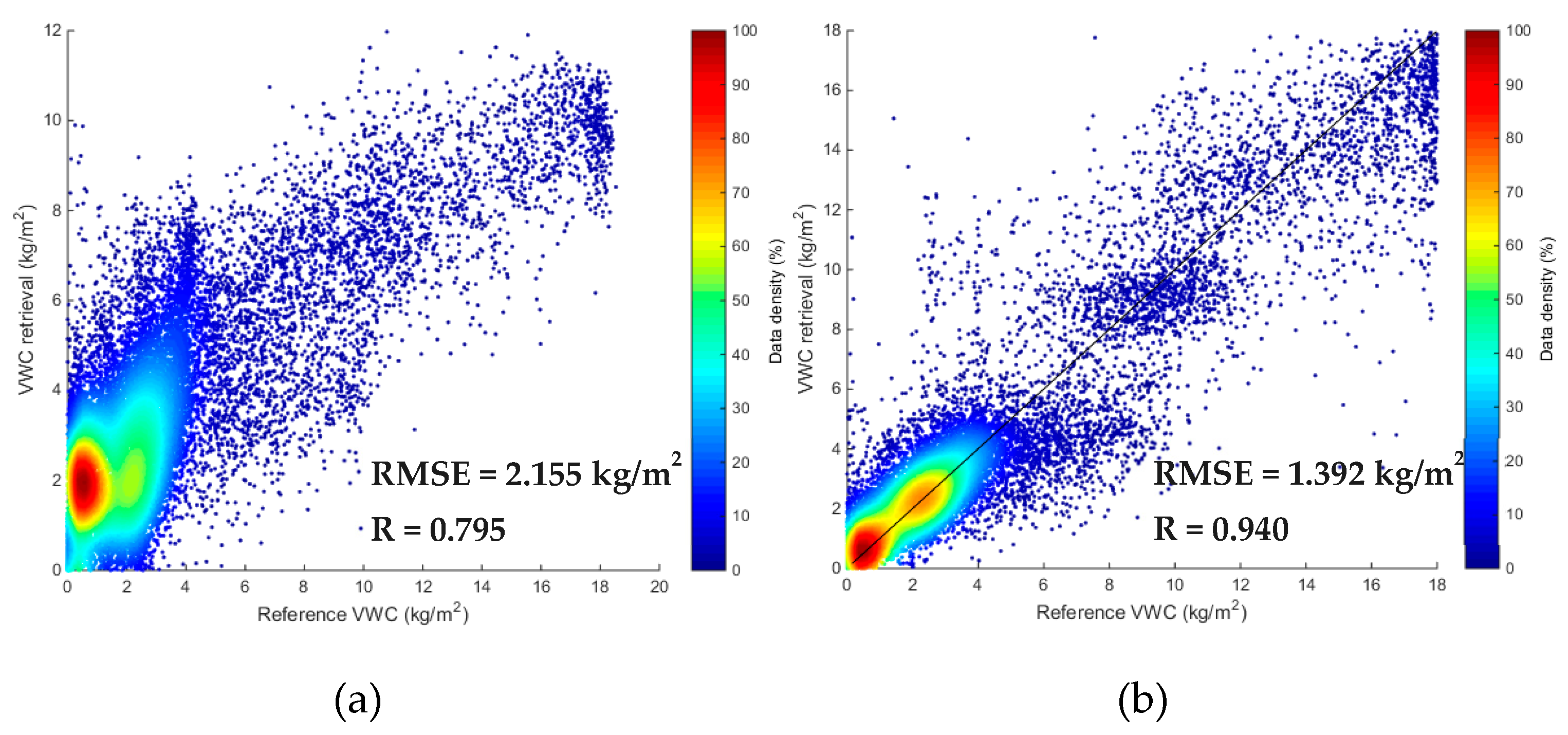
| Linear Model 5/Equation (20) | 1.580 | 0.619 | 2.155 | 0.795 | 32304 |
| ANN Model 5 | 0.844 | 0.252 | 1.392 | 0.940 | 34225 |
Disclaimer/Publisher’s Note: The statements, opinions and data contained in all publications are solely those of the individual author(s) and contributor(s) and not of MDPI and/or the editor(s). MDPI and/or the editor(s) disclaim responsibility for any injury to people or property resulting from any ideas, methods, instructions or products referred to in the content. |
© 2024 by the authors. Licensee MDPI, Basel, Switzerland. This article is an open access article distributed under the terms and conditions of the Creative Commons Attribution (CC BY) license (https://creativecommons.org/licenses/by/4.0/).
Share and Cite
Chen, F.; Liu, L.; Guo, F.; Huang, L. A New Vegetation Observable Derived from Spaceborne GNSS-R and Its Application to Vegetation Water Content Retrieval. Remote Sens. 2024, 16, 931. https://doi.org/10.3390/rs16050931
Chen F, Liu L, Guo F, Huang L. A New Vegetation Observable Derived from Spaceborne GNSS-R and Its Application to Vegetation Water Content Retrieval. Remote Sensing. 2024; 16(5):931. https://doi.org/10.3390/rs16050931
Chicago/Turabian StyleChen, Fade, Lilong Liu, Fei Guo, and Liangke Huang. 2024. "A New Vegetation Observable Derived from Spaceborne GNSS-R and Its Application to Vegetation Water Content Retrieval" Remote Sensing 16, no. 5: 931. https://doi.org/10.3390/rs16050931
APA StyleChen, F., Liu, L., Guo, F., & Huang, L. (2024). A New Vegetation Observable Derived from Spaceborne GNSS-R and Its Application to Vegetation Water Content Retrieval. Remote Sensing, 16(5), 931. https://doi.org/10.3390/rs16050931