Environmentally Induced Snow Transmittance Variations in the Photosynthetic Spectral Domain: Photobiological Implications for Subnivean Vegetation under Climate Warming Conditions

Abstract

Variations in the productivity of subnivean vegetation can substantially affect the ecology of regions more susceptible to increasing warming levels and lead to significant feedback effects on the global climate. Due to its importance, this topic is at the center of a broad scope of interdisciplinary studies supported by field and remote sensing observations. However, the current knowledge about environmental factors affecting the penetration of photosynthetically active radiation (PAR) through snow is still constrained by the paucity of transmittance data. In this work, we aim to further the understanding about these interconnected processes. We conduct a systematic investigation about the effects of independent and combined changes in key nivological characteristics, namely thickness, saturation, density and grain size, on snow transmittance in the photosynthetic spectral domain. Our investigation is carried out through controlled in silico (computational) experiments supported by measured radiometric data. Its outcomes unveil fundamental quantitative and qualitative trends related to the role played by these nivological characteristics on the spectral quality of transmitted PAR, which is quantified in terms of red to blue ($R/B$), red to far-red ($R/FR$) and blue to far-red ($B/FR$) ratios. These trends include increases in the $R/B$ ratio as well as decreases in the $R/FR$ and $B/FR$ ratios following thickness reductions or grain size increases, with opposite variations in these ratios being observed for saturation or density increases. Accordingly, the pairing of our findings with in situ and remotely collected information contributes to cement the scientific foundation required for the effective assessment of cause-effect loops linking accentuated vegetation greening to accelerated rates of snow cover recession.

1. Introduction

A substantial fraction of the Earth’s land surface is covered by snow. Besides having a major influence on the world’s radiation balance [1,2] and its atmosphere [3,4], snow represents an essential source of fresh water in different regions of the planet [5,6], and it is central for the sustainability of those regions’ ecosystems [7,8]. Accordingly, alterations in snow cover can have significant environmental ramifications [9]. In particular, they can lead to changes in vegetation phenology [10,11], which, in turn, can have a considerable impact on the global climate [6,12]. The ecological consequences of these interconnected biophysical processes are becoming more pronounced, notably in high latitude and high altitude biomes more affected by varying warming conditions [12,13].

Several studies, carried out in situ or remotely, have been reporting noticeable changes in the growing patterns of plant species in the Arctic and alpine regions in North America, Europe and Asia [6,13,14,15]. Despite these notable scientific efforts, however, there is still a considerable knowledge gap regarding the effects of snow cover alterations on the vegetation of these regions [12]. In fact, as alluded to by several research groups [9,12,16,17,18], the subnivean ecology of plants and their interactions with the covering snowpack remain largely overlooked in the related literature and, for all practical purposes, absent from climate impact models of high latitude and high altitude vegetation.

Most research initiatives involving the aforementioned processes are primarily based on the assessment of spectral radiation reflected by the affected regions, with a relatively small number of studies also including the quantification of light transmitted through snow cover. From a standard remote sensing point of view, it is comprehensible that more attention is given to reflected light [19,20,21,22], albeit the knowledge about factors affecting the light transmitted by target materials can be particularly relevant for challenging applications such as the remote detection of relatively thin snow layers [23,24]. From a broader scientific perspective, however, it is necessary to make inroads toward a more comprehensive understanding of the intertwined light transport mechanisms affecting snow reflectance and transmittance [1,2], notably with respect to the visible (photosynthetic) spectral domain. It is widely known that photosynthetically active radiation (PAR) is critical to the plants’ growth and to the equilibrium of their hosting biomes [16,25]. Accordingly, advances in this area would not only benefit remote sensing applications involving snow and vegetation interactions, but also drive transformative research efforts across several fields, from ecology and climatology to hydrology and agriculture, to name just a few.

Besides its pivotal participation in photosynthesis, PAR also markedly affects a myriad of important photobiological processes such as seed germination, photoperiodism and phototropism [8,26,27]. The extent of its effects on the subnivean vegetation depends not only on the amount (photon flux density or PFD [26]) of the transmitted light, but also on its spectral quality (distribution) [25,28,29]. For instance, a large number of plant species have photoblastic seeds, i.e., seeds whose germination is influenced (positively or negatively) by light [26,27]. Thus, PAR takes on a central photomorphogenic role by influencing the seeds’ germination timing [30], which impacts the survival of resulting seedlings and the plants’ fitness in subsequent life stages [26,29]. For many of these plant species, the breaking of seed dormancy is induced by red light (from 600–700 nm) and cancelled by far-red light (from 700–750 nm) [26].

Early field observations by Curl et al. [28] suggested that low levels of red light beneath relatively thin snow layers may also be sufficient for promoting algal blooms in the snowpack. Later, Richardson and Salisbury [25] postulated that the absence of red light or far-red light under thick snowpacks and their reappearance under thin snow layers could represent signals for regulating the development of lower and higher plants. It has also been suggested [18] that the low red to far-red ratio of transmitted light could suppress the emergence of plant organs under unfavourable temperature conditions. Conversely, high red to far-red ratios could stimulate their emergence under favourable conditions. This putative phenomenon would be similar to shade avoidance responses (e.g., petiole and internode elongation with the purpose of increasing light capture) also elicited by variations in the red to far-red ratios of radiation impinging on higher plants [27,31,32].

Recently, experiments by Kameniarová et al. [33] indicated that blue light (400–500 nm) can markedly contribute to the activation of cold tolerance and acclimation responses of plants. This aspect is consistent with previous empirical observations reporting that chlorophyll is synthesized under snow, and blue light increases its production [25,34]. Incidentally, this essential component of the photosynthesis process has its bands of absorption maxima located within the blue and red regions, and its band of absorption minima located within the green (500–600 nm) region of the light spectrum [35].

The scarcity of comprehensive studies on the effects of the environmentally induced variations on the spectral quality of PAR transmitted through snow cover may be explained by the intrinsic limitations of in situ measurements. For instance, while attempting to place sensors within a snow layer, one may inadvertently disturb the structure of the snowpack [2,17,18], which may affect the measurements’ reliability. Also, systematic investigations usually require specific variations in selected snow-specifying (nivological) characteristics while the others are kept fixed. Such a control is difficult to be achieved under field conditions in which the changes are elicited by environmental factors that may affect multiple nivological characteristics of the snowpack simultaneously. While such controlled experiments can be attempted under laboratory conditions, usually artificially prepared snow samples lack the morphological diversity (e.g., different grain sizes and shapes) found in natural samples [36], which limits the scope of the observations that can be derived from their outcomes. Moreover, experiments involving light transmission on scattering materials, conducted under field or laboratory conditions, have to face another challenging aspect, namely the control of incident illumination [1].

In this work, we systematically examine the impact that climate-elicited alterations in key morphological characteristics of snowpacks can have on the spectral quality of the transmitted PAR. More specifically, we focus on thickness (depth), density, grain size and saturation (fraction of the medium, or pore space, surrounding the snow grains occupied by water) alterations brought about by snow metamorphic processes (melting and settling) [16,28,37]. To overcome the technical constraints outlined earlier, we conducted controlled computational (in silico) experiments using a first-principles model for light interactions with snow, known as SPLITSnow (SPectral LIght Transport in Snow) [38]. It stochastically accounts for the complex structure of snow in order to output high-fidelity radiometric data (e.g., spectral reflectance and transmittance) for different illumination geometries.

The employed in silico investigation approach is grounded on measured radiometric and nivological data obtained for real snowpacks located in the Arctic [36]. We note that this is the region most affected by climate change effects, with a warming rate more accentuated than the global warming rate [12,39]. Moreover, this region is less prone to the presence of impurities (e.g., black carbon particles originating from human activities and industrial processes) that can significantly alter the absorption of light within a snowpack [2,16,25,40]. Thus, our choice of reference data also aimed to mitigate the introduction of undue biases in our present investigation focused on the transmittance of snow in its natural, uncontaminated state.

The outcomes of our investigation are expected to strengthen the knowledge foundation required for the effective interpretation of in situ and remote observations of biomes severely affected by snow cover alteration, and for the design of more robust climate impact models for those biomes [12,13]. Furthermore, although a number of works have examined how the transmittance of a snowpack is affected by changes in its nivological characteristics [2,18,25,28,33,37,40], there are aspects related to the role played by alterations in key snow parameters, such as density, that needed to be rectified. In this work, we also address these issues. Hence, the qualitative and quantitative observations derived from our findings also provide fundamental elements to be incorporated into broader interdisciplinary studies and remote sensing applications involving the ecological implications of snow and vegetation interactions [6,7,15] and their connections with global warming [9,12,14].

2. Materials and Methods

It is worth noting that measured datasets of light penetration in snow are usually available in terms of transmitted flux (radiant power) [25,28,37], or in terms of relative fractional readings relating the amount of radiant power reaching a certain depth with the amount of radiant power penetrating the snowpacks’s top boundary [17,18]. To date, hyperspectral measurements of transmittance, i.e., expressed by the ratio of transmitted to incident fluxes [41,42], not limited to a few spectral samples [1] and subjected to negligible contaminant-elicited spectral shifts [2], are still not readily available in the literature. This data paucity issue served as an additional motivation for our work, which may also be seen as a proof of concept for the generation of reliable hyperspectral transmittance data for snow, and prompted the use of the methodology described in the remainder of this section.

2.1. Snow Samples Characterization Data

In field studies on the penetration of light through snow, usually a given site is selected and measurements are conducted as the snow accumulation changes [2,18,25,28]. Similarly, in studies involving predictive simulations [43,44], one may choose to employ a representative snow sample with a characterization primarily based on the assignment of average values (provided in the related literature) to the material parameters. In this investigation, we elected to consider two distinct snow samples whose characterizations have a direct correspondence with real snowpacks for which measured reflectance datasets, to be used as baseline references, were readily available. As mentioned earlier, preference was given for data associated with snowpacks located in regions more sensitive to climate warming effects and less susceptible to contamination.

In order to meet the above guidelines, we searched for measured radiometric data accompanied by detailed descriptions of the target snowpacks. Accordingly, without loss of generality, we chose to use as baseline references for our investigation measured reflectance datasets obtained by Salvatori et al. [36] on the Svalbard island, in the Arctic. More specifically, these datasets were made available through the Snow and Ice Spectral Library (SISpec 2.0) as spectral files #6 and #195.

The measurements stored in each spectral file were respectively conducted at the Kulmodden (35 m above sea level) and Kiaerstranda (30 m above sea level) sites whose nivological characteristics were detailed reported. This supporting information was then employed to guide the assignment of appropriate values (presented in

Table 1. Parameter values employed in the characterization of the snow samples (A and B) considered in this investigation.

	Sample A	Sample B
Snow Parameters	Value	Value
Grain size range 1 ($\mathsf{\mu }$m)	200–300	150–800
Temperature (°C)	−8	−3
Thickness (cm)	18	10
Saturation 2 (%)	0	0
Density (kg/m3)	360	340
Facetness 3 range	0.05–0.25	0.1–0.4
Facetness mean	0.15	0.25
Facetness standard deviation	0.075	0.1
Sphericity 4 range	0.7–0.9	0.9–0.97
Sphericity mean	0.8	0.935
Sphericity standard deviation	0.1	0.05

¹ The snow grains are represented by prolate spheroids with a semi-major axis equal to c, and a semi-minor axis related to c by their sphericity [38,45]. As suggested in the UNESCO-IHP report on The International Classification for Seasonal Snow on the Ground, the “size of a grain or particle is its greatest extension” [46]. Accordingly, in our simulations, the size of the grain corresponds to $2c$, with c represented by a random variable with a uniform probability that allows for a configurable range. ² Fraction of a sample’s pore space occupied by water [38]. ³ Facetness ($f\in [0..1]$) equal to zero yields perfectly smooth grains [38]. It is represented in our simulations by a random variable with a normal probability distribution [38]. ⁴ Sphericity ($\Psi \in [0..1]$) equal to one yields perfectly spherical grains [38]. It is represented in our simulations by a random variable with a probability distribution previously employed for particulate materials [38,47].

) for the parameters used in the characterization of the virtual snow samples, henceforth simply referred to as Samples A and B, considered in our in silico experiments. The reader interested in more details about the selection of parameter values employed in the characterization of these samples is referred to Appendix A.

It is worth mentioning that Sample A has a thickness of 18 cm. This value approximately corresponds to the light penetration depth (LPD) of a typical snowpack, and it may also represent its photosynthesis compensation depth [28]. The former quantity is normally defined as the depth in which the incident light at the surface is reduced by ≥$99\%$, yielding transmittance values <$1\%$ [48,49,50], while the latter corresponds to the depth at which the rate of photosynthesis for an aquatic plant equals the rate of respiration by that plant [51].

Sample B, on the other hand, has a lower thickness (10 cm) and higher LPD. Its inclusion in our investigation was motivated by the possibility of expanding our quantitative and qualitative observations. It enabled us to assess changes in the spectral quality of PAR transmitted through samples with distinct morphological characteristics that could potentially lead to distinct optical behaviours.

2.2. In Silico Investigation Framework

2.2.1. Experimental Setup

The controlled in silico experiments presented in this work consisted primarily in the computation of directional-hemispherical reflectance and transmittance curves for the selected snow samples using the SPLITSnow model [38]. Its ray-optics formulation allows for a (light) ray interacting with a given snow sample to be associated with any wavelength (denoted by $\lambda$) within the spectral domain of interest. Accordingly, all modelled radiometric curves (from 400 to 750 nm) were computed considering a spectral resolution of 5 nm, with ${10}^6$ incident rays per $\lambda$. This number of rays cast by a virtual spectrophotometer [52] was selected to ensure asymptotically convergent radiometric readings.

For consistency with the SISpec measured radiometric datasets [36] employed as baseline references in this investigation, the modelled radiometric curves were obtained considering an angle of incidence of $0^{°}$ (with respect to the samples’ normal vector). We note that the SISpec measured radiometric datasets [36] correspond to reflectance factors calculated considering a hemispherical incidence geometry, with the a small acquisition sensor (optic fibre) positioned directly above (50 cm) the target surfaces. The modelled datasets, on the other hand, correspond to directional-hemispherical reflectances. This apparent discrepancy can be clarified as it follows.

Recall that reflectance can be defined as the ratio of reflected to incident fluxes [41,53], while reflectance (radiance) factor can be expressed as the ratio of the radiant flux reflected by the target surface to that which would be reflected into the same reflected-beam geometry by a diffuse surface irradiated in the exactly same way [54,55]. Based on the works of Judd [54] and Nicodemus [53,55], the directional-hemispherical reflectance and the hemispherical-directional reflectance factor quantities are considered numerically equivalent for a given direction as a direct consequence of Kirchhoff’s law [56] and the Helmholtz reciprocity principle [54]. Thus, for practicality, in studies involving the radiometric responses of materials characterized by a near-Lambertian behaviour, such as snow irradiated from an angle of incidence of $0^{°}$ [38,57], directional-hemispherical reflectance and hemispherical-directional reflectance factor can be used interchangeably [58,59].

We remark that light penetration measurements conducted in situ often rely on the insertion of sensors at different depths of a snowpack [17,18]. Considering the incoherent (diffuse) nature of light propagation through snow [1], such a setup may allow for light backscattered from a certain depth to be detected by a sensor placed at a shallower depth. This can result in a flux reading larger than that of the actual flux transmitted from the sample’s top boundary to the sensor’s depth. Since we are interested in the PAR reaching subnivean vegetation, instead of the PAR reflected by it, we employed a different setup. More specifically, we computed the transmittance values at the indicated thickness (equivalent to the depth of the samples’ bottom boundary). In other words, once a (light) ray exits a snow sample at the specified thickness (bottom depth), it is considered permanently propagated by the snow sample, i.e., it no longer contributes to the sample’s transmittance reading at that depth.

We note that our in silico experimental setup is consistent with other setups employed in field and quasi-laboratory campaigns. In some of those setups, the transmittance values are measured using a tunnel to place the measurement sensor at the bottom depth of the snowpack [25,34]. The values for different thicknesses (depths) are recorded as snow accumulates on a window (port) placed in the top of the tunnel located at snow-soil interface. Alternatively, the sensor is either positioned underneath a snow slab extracted from a snow bank and placed on a metal table [1], or on the top of a dark plywood platform in which snow accumulates following snowfalls [2]. Although, these setups are not suitable for the survey of a wide range conditions and depend on snowfall [2], they allow for radiometric readings to be obtained without disturbing the accumulated snow and creating pathways for spurious light transmission.

2.2.2. Experimental Phases

As the winter transitions to summer and the weather gets progressively warmer in high latitude and high altitude regions, snow melting and settling processes take place. These processes alter the morphological characteristics of the snow layers covering these regions. Their thickness decreases while their density, saturation level (associated with free water content) and grain size increase [28,37]. Accordingly, we organised our in silico experiments into three phases so that we could systematically examine the independent and concomitant impact of these environmentally elicited morphological alterations on the spectral quality of transmitted PAR.

Initially, in Phase I, we computed reflectance curves for the selected snow samples. We then compared the modelled curves with their measured counterparts provided by Salvatori et al. [36]. This enabled us to verify the plausibility of the snow characterization datasets (Table 1) and to establish reliable baselines for our transmittance experiments. Subsequently, in Phase II, we conducted transmittance experiments to assess the specific role played by changes in each of the affected nivological characteristics (parameters). Finally, in Phase III, we conducted experiments to examine their combined effects.

For the Phase II experiments, we considered the same relative changes for each given parameter for both samples. More specifically, for the thickness (denoted by t) experiments, we considered 25%, 50% and 75% reductions in the default values (Table 1). For the saturation (denoted by S) experiments, we considered four values (levels): 0% (default), 10%, 20% and 30%. For the density (denoted by d) experiments, we considered incremental changes of 80 kg/m³. Lastly, for the grain size range (denoted by $gsr$) experiments, we considered increments of 100 $\mathsf{\mu }$m in the samples’ average size calculated from their respective default $gsr$ values. We remark that all values assigned to S, d and $gsr$ are within the valid intervals reported for these nivological characteristics in the related literature [37,46,60].

For the Phase III experiments, we computed transmittance curves considering high values for d and $gsr$ parameters and curves considering low values for these parameters. More precisely, we assigned to d and $gsr$ the maximum and minimum values attributed to them in the Phase II experiments.

For each set of the Phase II and Phase III experiments, all parameters not subject to change were assigned the default values provided in Table 1 unless otherwise stated. For instance, the Phase II experiments involving changes in the samples’ saturation as well as the Phase III experiments were repeated considering a 75% reduction in the samples’ default thickness values. These additional experiments were conducted to further extend our scope of observations.

2.2.3. Spectral Ratios

To assess the alterations in the spectral quality of PAR transmitted through the snow samples considering the distinct scenarios outlined in Section 2.2.2, all transmittance experiments were accompanied by the calculation of selected spectral ratios of transmitted light: red to blue (denoted by $R/B$), red to far-red (denoted by $R/FR$) and blue to far-red (denoted by $B/FR$) [27]. These ratios were calculated using the following expressions [25]:

$$R/B=\frac{\tau \left(660\right)}{\tau \left(400\right)},$$

(1)

$$R/FR=\frac{\tau \left(660\right)}{\tau \left(730\right)},$$

(2)

and

$$B/FR=\frac{\tau \left(400\right)}{\tau \left(730\right)},$$

(3)

where $\tau \left(\lambda \right)$ denotes the transmittance at the wavelength $\lambda$ (in nm).

2.3. Fidelity and Reproducibility

Arguably, two aspects are essential for the validity of any in silico investigation, namely fidelity and reproducibility. Hence, it is relevant to point out that the predictive capabilities of the SPLITSnow model have been extensively evaluated through quantitative and qualitative comparisons with actual measured data and observations reported in the related literature [38,43,44]. Moreover, the degree of fidelity [61] of its predictions is further illustrated through our baseline experiments described in Section 3.1.

Regarding the reproducibility of our findings, we note that we made SPLITSnow accessible for online use [62] through our model distribution system [63]. Also, all supporting datasets, such as the spectral refractive indices for water and ice (Figure 1), employed in this work are openly available in a dedicated data repository [64].

It is worth noting that snow transmittance data can be obtained using models of snow and light interactions based on different simulations approaches. Given the intrinsic differences between such approaches (e.g., deterministic [67] versus non-deterministic [38]), the transmittance readings obtained by them may vary. Instead of using results provided by other models as references in our investigation, we strived to use measurements and empirical observations reported in the literature. After all, even if the readings provided by different models agree, their fidelity still needs to be assessed through comparisons with the “real thing” whenever this is feasible [61]. Incidentally, many of the existing models are designed primarily to provide reflectance readings. Perhaps, our investigation will motivate their designers to alter their formulation to allow for the straightforward computation of transmittance values, which could then be used to expand our findings. Clearly, such an undertaking is beyond the scope of the work described in this paper. The reader interested in comparisons of existing models is referred to a recent publication on this topic [68].

3. Results

3.1. Phase I—Baseline Responses

As it can be observed in the graphs presented in Figure 2, the reflectance curves computed for snow Samples A and B using the SPLITSnow model [38] show a close agreement with their measured counterparts provided by Salvatori et al. [36]. It has been indicated in the related literature [69] that root-mean-square errors (RMSE) below 0.03 indicate good spectrum reconstruction, notably for remote sensing applications. The RMSE values calculated for the reflectance curves obtained for Samples A and B were equal to 0.0033 and 0.0051, respectively. These aspects reiterate the plausibility of the employed snow characterization datasets (Table 1) and the fidelity of the predictions provided by our in silico experimental framework. Accordingly, we employed those datasets to obtain the sample’s transmittance curves in our subsequent experiments.

3.2. Phase II—Independent Effects

3.2.1. Thickness Changes

It has been reported that a reduction in the thickness of a snow layer leads to an increase in its transmittance, and such an increase is nonlinear [2,18,34]. Moreover, the transmittance values are higher in the blue-green region, and progressively lower in the red and far-red regions of the photosynthetic spectral domain [2,25]. As it can be observed in the graphs presented in Figure 3, the transmittance curves computed for Samples A and B present these traits.

The graphs presented in Figure 3 also show that the rate of transmittance increase is progressively higher with reduced thickness, with the transmittance curves tending to become flat within the blue and green regions as the samples get thinner. This behaviour is consistent with light transmission measurements performed for thin and thick snow covers [2,34]. It also aligns with the fact that the light traversing a snow layer tends to elicit a stronger blue-green hue as its thickness is increased, and a weaker blue-green hue otherwise [34,70]. These phenomena can be explained by the relatively higher levels of light absorption occurring at longer wavelengths within a snowpack [71,72,73].

It is worth noting that in the in situ fractional transmittance measurements performed by Robson and Aphalo [18], the readings obtained in the blue region at lower depths (associated with smaller thickness values) were significantly higher than the readings obtained for remainder of the PAR spectrum at the same depth. This apparent disparity with respect to the shape of the modelled transmittance curves presented in Figure 3 may be explained by the different measurement setup employed by Robson and Aphalo [18]. As previously outlined in Section 2.2.1, such a setup may also account for upward fluxes from depths higher (farther from the snow samples’ top surface) than that of the PAR detection sensor.

As for the impact of thickness reductions on the spectral quality of the transmitted PAR, they led to increases in the samples’ $R/B$ ratios, and decreases in their $R/FR$ and $B/FR$ ratios as depicted in

Table 2. Spectral ratios calculated for Samples A and B considering the effects of thickness (t, in cm) changes on their transmittance curves (Figure 3).

Sample A					Sample B
t	$R/B$	$R/FR$	$B/FR$		t	$R/B$	$R/FR$	$B/FR$
18.0	0.16	5.49	33.84		10.0	0.54	1.94	3.55
13.5	0.30	3.03	10.11		7.5	0.71	1.55	2.21
9.0	0.56	1.87	3.32		5.0	0.87	1.25	1.45
4.5	0.88	1.23	1.39		2.5	0.98	1.07	1.09

. Furthermore, the $B/FR$ ratios presented the largest variations. Again, this aspect may be explained by the distinct levels of light absorption taking place at the opposite ends of the PAR spectrum [71,72]. Since the absorption levels of blue light are lower than those of far-red light, the quantification of the former (in terms of PFD) tends to be more sensitive to thickness changes.

3.2.2. Saturation Changes

The presence of water in a snow sample’s pore space affects the propagation of light through distinct light attenuation mechanisms. It increases the probability of light being scattered/refracted from the ice grains to the pore space by reducing the refractive index differences between the grains and their surrounding medium. In addition, the presence of water increases the probability of red and far-red light traversing the pore space being absorbed since the extinction coefficient of water markedly increases toward the red-end of the PAR spectrum (Figure 1b).

The net effect of these mechanisms is a trend towards a transmittance increase in the blue and green regions, and a transmittance decrease in red and far-red regions. As it can be observed in the graphs presented in Figure 4, the modelled transmitted curves depict this trend, albeit the observed changes have a small magnitude due to the relatively low amount of light reaching the bottom boundary of the samples at their specified default thickness values (Table 1). It can also be observed that the transition from the reduced to the increased transmittance profiles is located in different spectral bands for each sample. While for Sample A it is located within a spectral band in the green region, for Sample B its located within a spectral band in the red region. This difference may be attributed to the distinct morphological characteristics of the samples, and to the effects that changes in these characteristics can have on the samples’ optical properties.

In

Table 3. Spectral ratios calculated for Samples A and B considering the effects of saturation (S, in %) changes on their transmittance curves (Figure 4).

Sample A					Sample B
S	$R/B$	$R/FR$	$B/FR$		S	$R/B$	$R/FR$	$B/FR$
0	0.16	5.49	33.84		0	0.54	1.94	3.55
10	0.12	11.98	102.20		10	0.51	2.58	4.99
20	0.10	20.10	203.31		20	0.49	3.10	6.29
30	0.09	25.71	289.55		30	0.48	3.56	7.39

, we provide the spectral ratios computed for Samples A and B considering the effects of saturation changes on their transmittance curves (Figure 4). For both samples, the increase of their saturation levels led to the decrease of their $R/B$ ratios and the increase of their $R/FR$ and $B/FR$ ratios. The large values calculated for the $B/FR$ ratios of Sample A with respect to the high saturation levels may be explained by the magnification of numerical values occurring when diving by small numbers, which are represented in this case by transmittance readings approaching zero in the far-red region (Figure 4a).

To broaden our scope of observations, we repeated the saturation experiments considering a 75% reduction in the samples’ default thickness values. The resulting transmittance curves are presented in Figure 5. Trends similar to those verified for the default thickness values can be observed, namely a transmittance increase for shorter wavelengths and a transmittance reduction for longer wavelengths. However, since there is more light reaching the samples’ bottom border, the transmittance changes are more noticeable for the thinner versions of the samples. Moreover, the transition between the two behaviours was located in narrower spectral bands closer to the end of the spectral domain of interest. Again, the transition position was not the same for both samples. While for Sample A the host narrow band was located between the red and far-red regions, for Sample B it was located within the far-red region.

Despite the differences between transmittance changes brought about by the increase in saturation in the thinner versions of the samples with respect to changes reported for their thicker (default) versions, the corresponding spectral ratios presented in

Table 4. Spectral ratios calculated for Samples A and B considering the effects of saturation (S, in %) changes on their transmittance curves (Figure 5) and their default thickness values reduced by 75%.

Sample A					Sample B
S	$R/B$	$R/FR$	$B/FR$		S	$R/B$	$R/FR$	$B/FR$
0	0.87	1.23	1.42		0	0.98	1.07	1.09
10	0.84	1.39	1.65		10	0.97	1.09	1.13
20	0.82	1.54	1.88		20	0.96	1.13	1.17
30	0.80	1.66	2.07		30	0.95	1.15	1.21

depict the same qualitative trends. More precisely, for both samples, the increase of their saturation level led to the decrease of their $R/B$ ratios and the increase of their $R/FR$ and $B/FR$ ratios. Quantitatively, however, the variations in the $R/FR$ and $B/FR$ ratios were noticeably smaller than those associated with the same spectral ratios calculated considering the samples default thickness values.

3.2.3. Density Changes

As indicated in the graphs presented in Figure 6, the increase in the samples’ density led to a decrease in their transmittance. This behaviour, also noted in quasi-laboratory experiments [2], can be associated with the accentuation of light detour effects [35,74,75] that can lengthen the path traversed by light, increasing the probability of attenuation events [28]. Furthermore, the graphs presented in Figure 6 show that the transmittance decrease observed for both samples is nonlinear, being progressively lower with increased density.

Compared to the saturation changes (Figure 4), the density changes considered in our experiments resulted in more noticeable alterations in the transmittance curves (Figure 4) considering the samples’ default thicknesses. The qualitative trends observed in the variations of the spectral ratios associated with density changes were the same as those associated with saturation changes, however. More precisely, as presented in

Table 5. Spectral ratios calculated for Samples A and B considering the effects of density (d, in kg/m³) changes on their transmittance curves (Figure 6).

Sample A					Sample B
d	$R/B$	$R/FR$	$B/FR$		d	$R/B$	$R/FR$	$B/FR$
200	0.48	2.07	4.30		180	0.87	1.29	1.52
280	0.29	3.28	11.41		260	0.69	1.54	2.21
360	0.16	5.49	33.84		340	0.55	1.94	3.55
440	0.07	8.53	116.98		420	0.41	2.45	5.90

, the increase in density also led to the decrease of the $R/B$ ratios and the increase of the $R/FR$ and $B/FR$ ratios for both samples. Furthermore, similar to what happened in the saturation experiments, the large values calculated for the $B/FR$ ratio of Sample A with respect to the highest density considered in the experiments may also be explained by the aforementioned numerical magnification issue (Section 3.2.2) involving transmittance values approaching zero in the far-red region (Figure 6a).

3.2.4. Grain Size Changes

Laboratory experiments [76,77] carried out on different soil samples have shown that their transmittance increases with increased soil grain (particle) size. In the case of particulate materials like soils, larger grains are less likely to scatter light [48]. Thus, the consequence of grain size increase is a reduction in light attenuation, which leads to an increase in transmittance for a given thickness. From an analytical point of view, larger snow grains are also associated with lower levels of light attenuation [40]. Thus, the transmittance of snow is also expected to have an inverse relationship with the size of their constituent grains as reported for other particulate materials. Indeed, this behaviour was verified by our in silico experiments, i.e., the increase in the samples’ grain size range led to higher transmittance values for both samples as depicted in the graphs presented in Figure 7.

The increase in the grain size range also resulted in variations in the associated spectral ratios, albeit markedly distinct from those observed in the previous experiments. More precisely, as indicated in

Table 6. Spectral ratios calculated for Samples A and B considering the effects of grain size range ($gsr$, in $\mathsf{\mu }$m) changes on their transmittance curves (Figure 7).

Sample A					Sample B
$gsr$	$R/B$	$R/FR$	$B/FR$		$gsr$	$R/B$	$R/FR$	$B/FR$
200–300	0.16	5.49	33.84		150–800	0.54	1.94	3.55
300–400	0.25	3.53	14.24		350–800	0.76	1.43	1.88
400–500	0.33	3.06	9.29		550–800	0.82	1.31	1.59
500–600	0.88	2.50	6.52		750–800	0.84	1.26	1.49

, the increase in the samples’ grain size range led to the increase of their $R/B$ ratios and the decrease of the $R/FR$ and $B/FR$ ratios.

3.3. Phase III—Combined Effects

As indicated by the outcomes of the Phase II experiments, the nivological characteristics particularly changed by snow melting and settling processes, namely density and grain size, have opposite effects on the spectral quality of transmitted PAR when their respective changes are considered separately. However, we remark that concomitant changes of these characteristics have been observed during those natural processes, with the increase in the density of a snowpack’s being accompanied by the increase in the size of its constituent grains [37]. To investigate the net effect of these concomitant changes, we compared the transmittance curves obtained considering the minimum and maximum values assigned to the related snow parameters, d and $gsr$, in the Phase II experiments.

As it can be verified in the graphs presented in Figure 8, the simultaneous increase in density and grain size resulted in the decrease of transmittance in the lower portion of PAR spectrum, and in the increase in the higher portion for both samples. While the transition point was located within the 550–600 nm band for Sample A, it was located within the 650–700 nm band for Sample B. The presence of water, which can also occur during the snow metamorphic processes [37], slightly accentuated these trends for both samples.

These aspects indicated that the effects of concomitant density and grain size changes on snow transmittance are not uniform across the PAR spectrum, and their spectral dependency can vary depending on the nivological characteristics of a given snowpack. The trends observed for the samples’ spectral ratios, which are presented in

Table 7. Spectral ratios calculated for Samples A and B considering the combined effects of density (d, in kg/m³), grain size range ($gsr$ in $\mathsf{\mu }$m) and saturation (S in %) changes on their transmittance curves (Figure 8).

Sample A							Sample B
d	$gsr$	S	$R/B$	$R/FR$	$B/FR$		d	$gsr$	S	$R/B$	$R/FR$	$B/FR$
200	200–300	0	0.50	2.17	4.36		180	150–800	0	0.85	1.27	1.40
440	500–600	0	0.26	3.57	13.70		420	750–800	0	0.78	1.40	1.79
440	500–600	30	0.19	12.85	66.32		420	750–800	30	0.70	2.16	3.07

, were the same, however. More specifically, the concomitant increase in density and grain size led to the decrease of the samples’ $R/B$ ratios, and the increase of their $R/FR$ and $B/FR$ ratios. These behaviours were also observed when we considered the presence of water in the samples’ pore space.

We remark that during the melting and settling processes, the thickness of a snow cover may also be reduced [28]. Accordingly, we repeated the previous experiments considering a 75% reduction in the samples’ default thickness values (Table 1). As a result, the effects on the samples’ transmittance curves were altered both quantitatively and qualitatively. More precisely, as depicted in the graphs presented in Figure 9, the concomitant increase in density and grain size led to a transmittance increase across the blue-red region for both samples. In the case of Sample B, this increase was also verified in the far-red region. Furthermore, the magnitude of the transmittance variations was larger than that observed considering the samples’ default thickness values (Figure 8).

Like in the previous experiments considering the samples’ default thickness values, the presence of water affected the transmittance variations. For both samples, it accentuated the transmittance increase in the blue-red region. However, for the far-red region, it counteracted the effects of concomitant increase in density and grain size. In fact, for Sample A, it has led to the decrease of transmittance in the far-red region.

As for the corresponding spectral ratios, which are presented in

Table 8. Spectral ratios calculated for Samples A and B considering the combined effects of density (d, in kg/m³), grain size range ($gsr$ in $\mathsf{\mu }$m) and saturation (S in %) changes on their transmittance curves (Figure 9) when their default thickness values are reduced by 75%.

Sample A							Sample B
d	$gsr$	S	$R/B$	$R/FR$	$B/FR$		d	$gsr$	S	$R/B$	$R/FR$	$B/FR$
200	200–300	0	0.98	1.08	1.10		180	150–800	0	1.01	1.02	1.01
440	500–600	0	0.92	1.17	1.26		420	750–800	0	1.00	1.02	1.02
440	500–600	30	0.88	1.40	1.59		420	750–800	30	0.99	1.09	1.11

, they depicted the same trends reported for the samples when we considered their default thickness values. More explicitly, the concomitant increase in density and grain size led to the decrease of their $R/B$ ratios, and the increase of their $R/FR$ and $B/FR$ ratios. Furthermore, these trends were also verified when we considered the presence of water in the samples’ pore space. However, while the magnitude of the transmittance variations was more accentuated for the thin version of the samples, the magnitude of spectral ratios’ variations was markedly less significant.

4. Discussion

Despite the important connections between environmentally induced alterations in snow PAR transmission profiles and changes in subnivean vegetation, which can lead to pivotal feedback effects [12,78] on the planet’s climate patterns and on the sustainability of its ecosystems [6,13], there is a noticeable paucity of measured transmittance data to support comprehensive studies in this area. 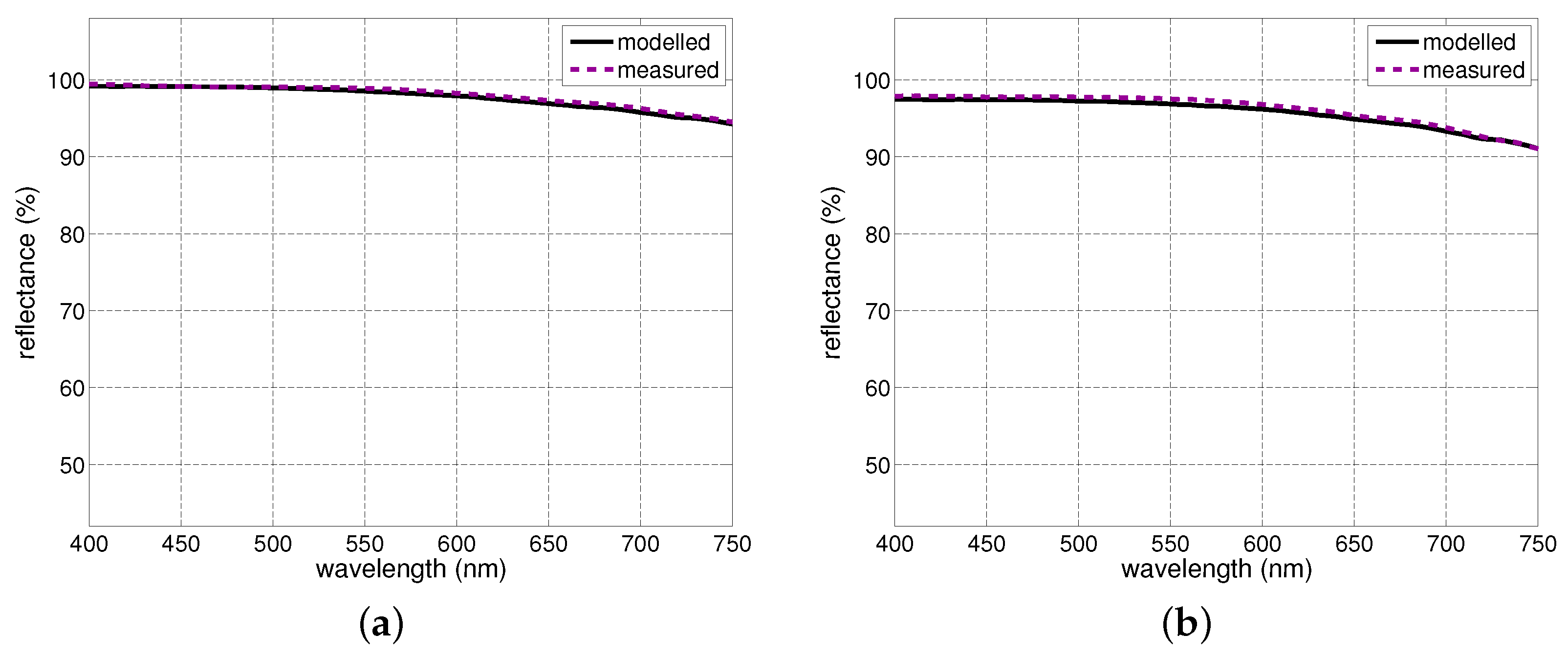Such studies are needed to further the current understanding about the impact of snow cover alterations on vegetation [9,12,15]. Thus, to systematically examine those connections while coping with measured data constraints, we employed an in silico experimental approach and used available reflectance measurements for snow to establish baseline references (Section 3.1) for our investigation.

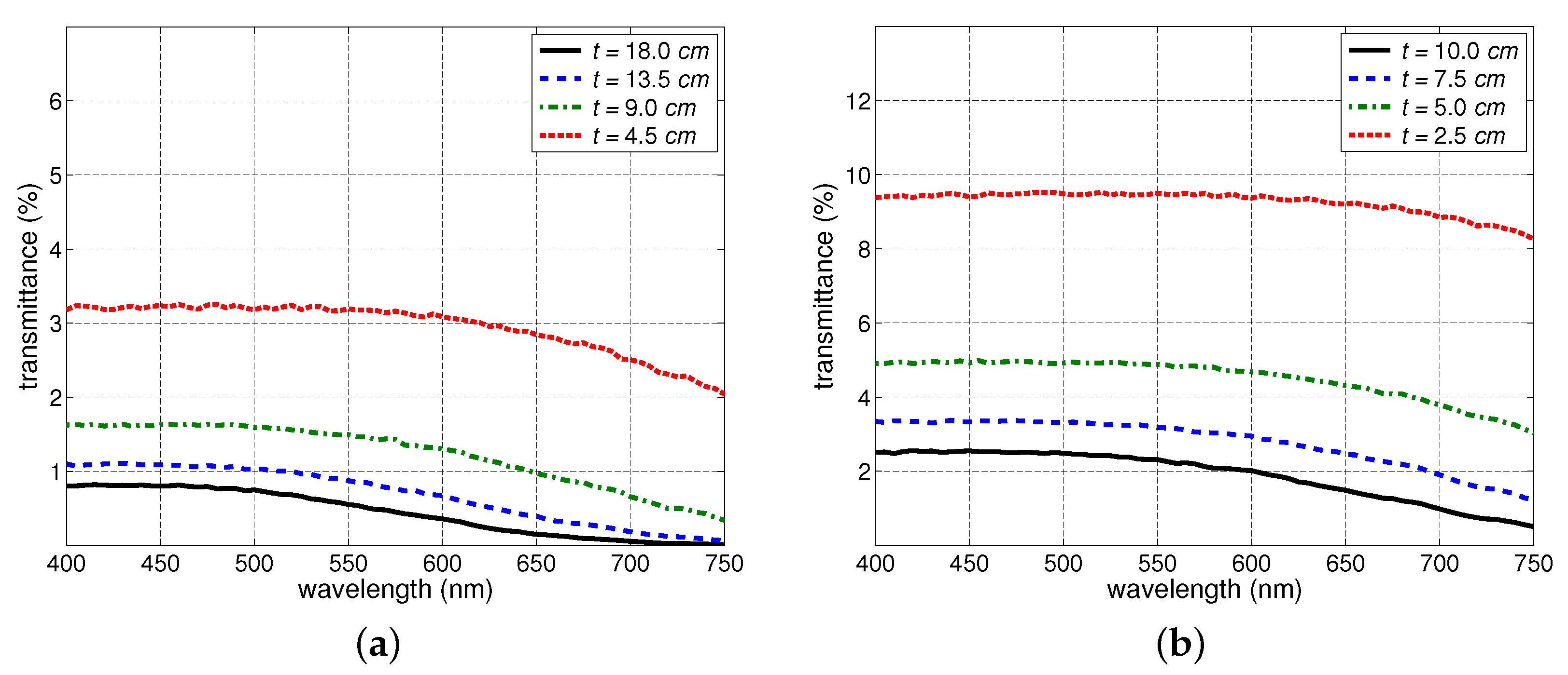
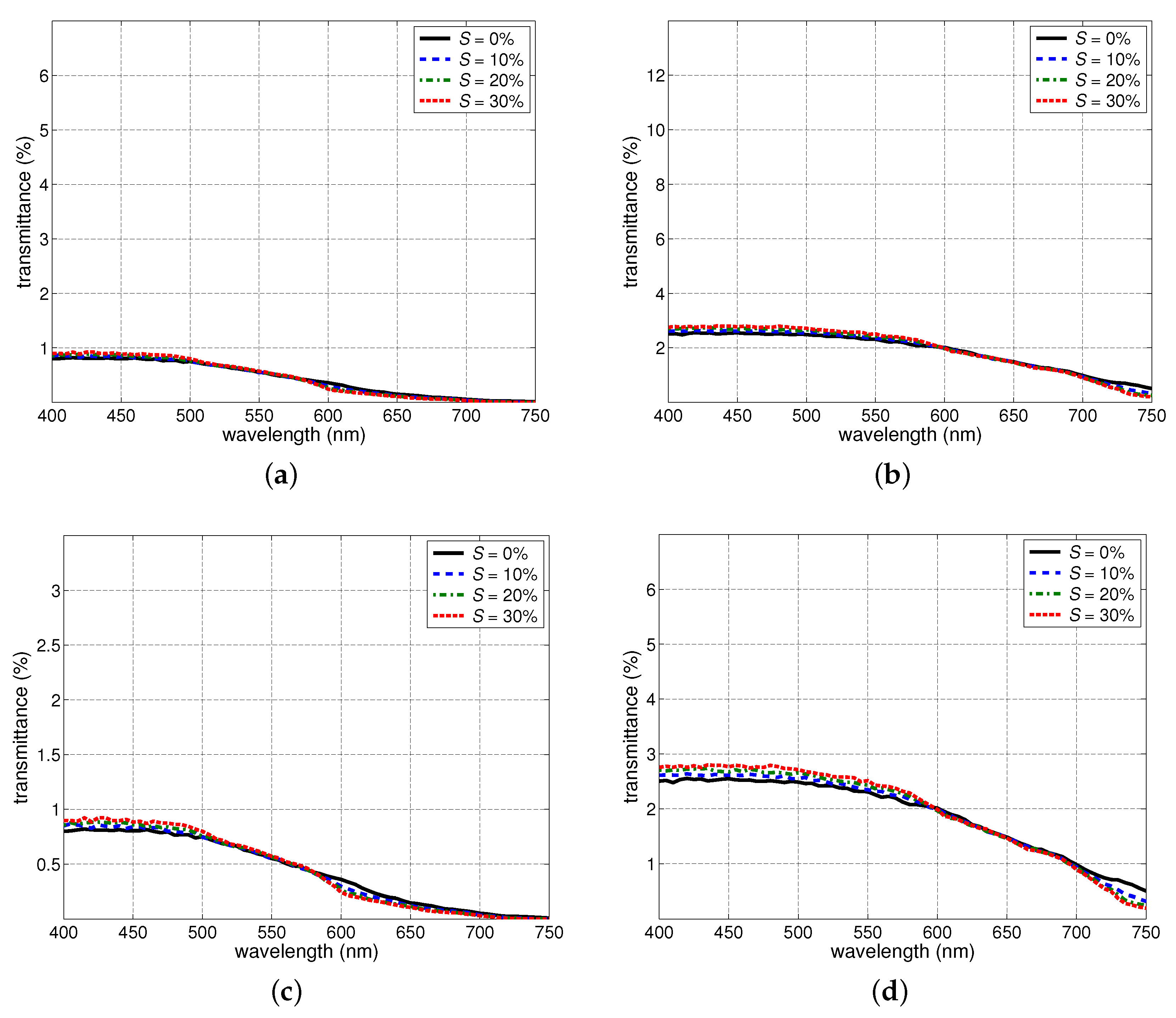
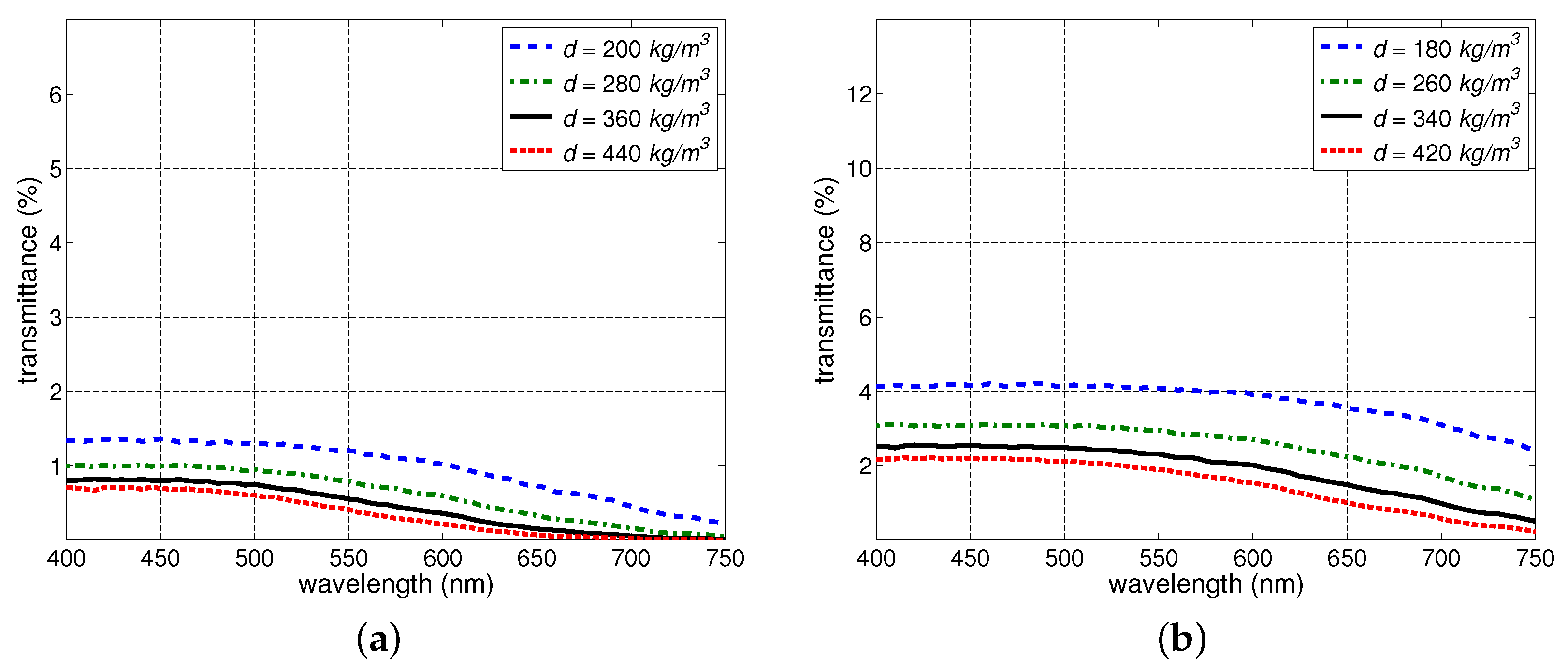
Initially, we methodically examined the effects of independent changes in snow thickness, saturation, density and grain size (Section 3.2). The transmittance changes specifically elicited by each of these snow characteristics were consistent with empirically-based observations reported in related works on light interactions with granular materials. In concise terms, the reduction in thickness led to a nonlinear transmittance increase, the increase in saturation led to a transmittance increase in the lower end of the PAR spectrum and an increase in the upper end, the increase in density led to a transmittance decrease, and the increase in grain size led a transmittance increase.

As mentioned in Section 2.1, we have considered as references two snow samples with distinct characteristics in our investigation. It may be argued, that the use of a larger number of snow samples can lead to quantitative variations in our observations, i.e., transmittance curves with distinct magnitudes. However, we remark that our focus was on qualitative trends. These are likely to be preserved since the employed samples have typical characterizations. In fact, as mentioned earlier, our observations were consistent with trends empirically verified for snow and other granular materials with distinct characteristics. Nonetheless, there is certainly room for the future extension of our investigation to samples characterized by more significant variations from the norm such as those containing noticeable amounts of impurities.

It is also worth noting that density plays a particularly relevant role in environmental studies involving the effects of snow cover variations in subnivean vegetation and soil [16,79], as well as in estimations of SWE (snow water equivalent) quantities [22]. Our findings indicate that an independent increase in the density of a snowpack leads to a decrease in its PAR transmittance. Although this relationship is consistent with empirically-based observations reported in the literature (Section 3.2.3), it has been stated in a number of publications [17,18,25,28] that transmittance of a snowpack increases with increased density. Incidentally, none of those works carried actual controlled experiments on the independent effects of density changes on snowpack’s transmittance.

The explanation for this apparent divergence lies on how the field observations reported in the seminal work by Gerdel [37] have been interpreted and cited in those subsequent publications. For instance, Robson and Aphalo [18] stated that snow transmittance increases with increased density citing the work by Richardson and Salisburry [25], while Saarinen et al. [17] mentioned the same transmittance-density relationship citing the work of Curl et al. [28]. Richardson and Salisburry [25], in turn, cited the works by Curl et al. [28] and Gerdel [37] when they mention rises in light transmission through a snowpack following increases in its density, while Curl et al. [28] themselves cited the work of Gerdel [37] when they made the same statement.

Upon a closer examination of Gerdel’s field observations [37], a few elucidative aspects stand out. First, his measurements did not include spectral distributions. Instead, they corresponded to the total amount of radiance from 250 to 3000 nm penetrating the snowpack. Second, indeed Gerdel [37] initially mentioned that the amount of transmitted radiation increases with increase density. However, while describing his experiments in more detail, he also reported that the increase in density was accompanied by a substantial increase in grain size and, in some measurement instances, it was also accompanied by an increase in the percentage of free water (associated with the snowpack’s saturation level). More recently, Perovich [2] suggested that density might have been just a proxy for other snow characteristics, notably grain size, in previous investigations of its relationship with snow optical properties.

We remark that the outcomes of our Phase III experiments (Section 3.3) showed that a concomitant increase in density and grain size can lead to a transmittance increase in the PAR spectral domain, and such an increase can be further affected by the presence of water in the samples’ pore space. Hence, as indicated by our density related findings, presented in Section 3.2.3 and Section 3.3, the effects of density changes on the snow transmittance may vary depending whether or not these changes are accompanied by significant alterations in the other key nivological characteristics, namely, grain size, saturation and thickness.

The data scarcity issue highlighted earlier is even more severe with respect to the spectral distribution of the transmitted PAR and its quantification in terms of photobiologically relevant spectral ratios, notably $R/B$, $R/FR$ and $B/FR$. The extent of the impact of individual or combined changes in snow characteristics on these ratios have not been examined in the related literature to date. In our investigation, we specifically aimed to address this knowledge gap. Recall that, as snow melting and settling processes take place, the thickness of a snowpack decreases, while its saturation, density and grains’ size range increase [28,37]. Accordingly, we were particularly interested in these environmentally elicited changes to the examined nivological characteristics.

The outcomes of our Phase II experiments involving independent changes in the samples’ nivological characteristics (Section 3.2) brought out definite trends, which are concisely depicted in

Table 9. Summary of alterations in the $R/B$, $R/FR$ and $B/FR$ spectral ratios of PAR transmitted through the examined snow samples considering independent changes in their nivological characteristics (Phase II experiments). The symbols ↓ and ↑ represent decreases and increases, respectively.

Characteristic	Change	$\mathit{R}/\mathit{B}$	$\mathit{R}/\mathit{FR}$	$\mathit{B}/\mathit{FR}$
Thickness	↓	↑	↓	↓
Saturation	↑	↓	↑	↑
Density	↑	↓	↑	↑
Grain Size	↑	↑	↓	↓

. More explicitly, while thickness reductions and grain size increases led to increases in the $R/B$ ratio and decreases in the $R/FR$ and $B/FR$ ratios, the increases in saturation and density led to opposite effects on these ratios. Moreover, changes in a specific parameter leading to an increase in the $R/B$ ratio were accompanied by a decrease in the corresponding $RF$ and $B/FR$ ratios, and vice-versa. We note that these trends were observed for both snow samples.

Recall that variations in the $R/B$, $R/FR$ and $B/FR$ ratios may act as signals to prompt the activation and/or accentuation of biophysical processes that can directly affect the development of subnivean vegetation (Section 1). These interconnected photobiological mechanisms include the rise in chlorophyll production associated with decreases in the $R/B$ ratios [25,34], the breaking of seed dormancy and the emergence of plant organs associated with increases in the $R/FR$ ratios [18,26], as well as the reduction of cold tolerance and acclimation responses associated with decreases in the $B/FR$ ratios [25,33]. Hence, our findings suggest that, although thinner snowpacks and snowpacks formed by larger grains are more likely to provide more favourable conditions for the growth of subnivean vegetation, they are less likely to contribute to the gemination of subnivean seeds and the emergence of subnivean plants organs sensitive to increases in the $R/FR$ ratios. On the other hand, denser snowpacks and wet snowpacks are likely to have the opposite effects on subnivean vegetation.

As previously noted (Section 2.2.2), the changes in the examined nivological characteristics are likely to occur concomitantly as a snowpack undergoes melting and settling processes. The outcomes of our Phase III experiments (Section 3.3), in which we considered this possibility, also brought out definite trends summarized in

Table 10. Summary of alterations in the $R/B$, $R/FR$ and $B/FR$ spectral ratios of PAR transmitted through the examined snow samples considering concomitant increases in their density, grain size range and saturations values (Phase III experiments). The alterations are provided with respect to the samples’ default and reduced thickness values, with the symbols ↓ and ↑ representing decreases and increases, respectively.

Thickness	$\mathit{R}/\mathit{B}$	$\mathit{R}/\mathit{FR}$	$\mathit{B}/\mathit{FR}$
Default	↓	↑	↑
Reduced	↓	↑	↑

. More specifically, a thickness reduction accompanied by an increase in saturation, density and grain size is likely to lead to the decrease of the $R/B$ ratios and the increase of the $R/FR$ and $B/FR$ ratios. Again, these trends were observed for both snow samples. Hence, our findings also suggest that, as snow metamorphic processes take place, the PAR traversing a snowpack is more likely to accentuate the production of chlorophyll as well as the cold tolerance and acclimation responses of subnivean plants. It may also promote the germination of photoblastic seeds and the emergence of plant organs, particularly those belonging to subnivean species sensitive to increases in the $R/FR$ ratios. Hence, our findings are aligned with recently reported observations on increasing vegetation productivity, or greening [7,13], following snow cover recession, notably in high latitude and high altitude regions more susceptible to climate warming effects on snow melting and settling processes [12,14].

We note that the greening phenomenon has been the object of a wide gamut of interdisciplinary studies supported by field and remote sensing observations [6,9,13,14,15,78]. Besides being driven by environmental factors and significantly affecting local biomes, it can also result in cause–effect loops with a direct impact on global climate and ecology [6,12]. For instance, the greening elicited by snow cover reduction accentuates radiation exchanges, leading to faster snowmelt and reduced snow cover, which, in turn, not only continues to increase greening, but also reduces the amount of melt water available for the plants during their growing stages [13,14]. Hence, at a critical, tipping point, vegetation productivity can decrease, negatively impairing the biodiversity of the affected regions, which may experience accelerated rates of extinction for local species [12]. Such a decrease in vegetation productivity can also negatively reinforce climate changes by reducing the landscapes’ reflectance (albedo) and subsurface thermal insulation [13,15].

To effectively tackle the complexity of these scenarios and their climatological and ecological ramifications, it is necessary to further the current understanding about the underlying photobiological mechanisms of those fundamental processes. Viewed in this context, the in silico experimental framework employed in this investigation can also be seen as a predictive platform to be used to complement in situ and remote observations and, consequently, expedite the hypothesis generation and validation cycles of future research initiatives on this timely and far-reaching scientific topic.

5. Conclusions

In this investigation, we conducted controlled in silico experiments to systematically examine the impact that environmentally elicited changes in key snow characteristics, namely thickness, saturation, density and grain size, can have on the spectral quality of transmitted PAR, quantified in terms of $R/B$, $R/FR$ and $B/FR$ spectral ratios. Our findings brought out specific trends associated with independent and concomitant changes in the examined nivological characteristics. In particular, they indicate that, while an increase in density accompanied by an increase in grain size can lead to a transmittance increase, an increase in density alone results in a transmittance decrease. These different behaviours have been overlooked in the related literature.

Our findings also suggest that the concomitant changes in snow thickness, saturation, density and grain size that take place during snow melting and settling processes affect the examined spectral ratios associated with the transmitted PAR. Furthermore, the net effect of their influence in the spectral quality of the transmitted PAR tends to favour an increase in the productivity of subnivean vegetation. More specifically, the outcomes of in silico experiments provide tangible elements that can be incorporated into large scale studies, involving both field and remote observations, on the feedback effects of greening in the ecology of high latitude and high altitude regions, more affected by increasing warming conditions, and in the global climate. As future work, we plan to extend our investigation to snow-vegetation interactions occurring in regions more exposed to climate altering factors prompted by human activities such as the burning of fossil fuels and industrial pollution. We also believe to be worthwhile to explore the ramifications of our investigation from a distinct perspective involving the calculation of indices such as SWE.

As any in silico investigation, the outcomes of this work are still subject to in situ confirmation as measured hyperspectral transmittance data for snow becomes available. We remark that the use of a predictive first-principles in silico framework was also prompted by the scarcity of measured snow transmittance data. This brings out an important issue, the need not only for more measured data, but also for data of good quality, i.e., radiometric data with a fine spectral resolution, properly measured (e.g., with negligible disturbances to the snowpack) and accompanied by a detailed description of the target snowpack and the measurement conditions. We believe that the pairing of data obtained through in situ experiments and remote sensing observations with in silico data obtained through high-fidelity simulations can be instrumental for advancing the current knowledge about snow and vegetation interactions. This, in turn, is essential for increasing the effectiveness of procedures and technologies aimed at the monitoring and management of adverse climate effects on the planet’s ecological sustainability.

References

1. Beaglehole, D.; Ramanathan, B.; Rumberg, J. The UV to IR transmittance of Antarctic snow. J. Geophys. Res. 1998, 103, 8849–8857. [Google Scholar] [CrossRef]
2. Perovich, D. Light reflection and transmission by a temperate snow cover. J. Glaciol. 2007, 53, 201–210. [Google Scholar] [CrossRef]
3. Dominé, F.; Shepson, P. Air-snow interactions and atmospheric chemistry. Science 2002, 297, 1506–1509. [Google Scholar] [CrossRef]
4. Strack, J.; Liston, G.; Pielke, R., Sr. Modeling snow depth for improved simulation of snow-vegetation-atmosphere interactions. J. Hydrometeorol. 2004, 5, 723–734. [Google Scholar] [CrossRef]
5. Barnett, T.; Adam, J.; Lettenmaier, D. Potential impacts of a warming climate on water availability in snow-dominated regions. Nature 2005, 438, 303. [Google Scholar] [CrossRef]
6. Zhang, X.; Sa, C.; Hai, Q.; Meng, F.; Luo, M.; Gao, H.; Zhnag, H.; Yin, C.; Zhang, Y.; Sun, H. Quantifying the effects of snow on the beginning of vegetation growth in the Mongolian plateau. Remote Sens. 2023, 15, 1245. [Google Scholar] [CrossRef]
7. Walker, D.; Halfpenny, J.; Walker, M.; Wessman, C. Long-term studies of snow-vegetation interactions. BioScience 1993, 43, 287–301. [Google Scholar] [CrossRef]
8. Walker, D.; Billings, W.; De Molenaar, J. Snow-Vegetation Interactions in Tundra Environments. In Snow Ecology: An Interdisciplinary Examination of Snow Covered Ecosystems; Walker, D., Ed.; Cambridge University Press: Cambridge, UK, 2001; pp. 266–324. [Google Scholar]
9. Hao, X.; Li, H.; Wang, X.; Wang, X.; Huang, X.; Bi, J. An overview of remote sensing for mountain vegetation and snow cover. Remote Sens. 2022, 14, 5694. [Google Scholar] [CrossRef]
10. Cooper, E.; Dullinger, S.; Semenchuk, P. Late snowmelt delays plant development and results in lower reproductive success in High Artic. Plant Sci. 2011, 180, 157–167. [Google Scholar] [CrossRef] [PubMed]
11. Sanders-DeMott, R.; McNellis, R.; Jabouri, M.; Templer, P. Snow depth, soil temperature and plant-herbivore interactions mediate plant response to climate change. J. Ecol. 2018, 106, 1508–1519. [Google Scholar] [CrossRef]
12. Niittynen, P.; Heikkinen, R.; Luoto, M. Snow cover is a neglected driver of Artic biodiversity loss. Nat. Clim. Chang. 2018, 8, 997–1003. [Google Scholar] [CrossRef]
13. Rumpft, S.; Gravery, M.; Brönnimann, O.; Luoto, M.; Cianfrani, C.; Mariethoz, G.; Guisan, A. From white to green: Snow cover loss and increased vegetation productivity in the European Alps. Science 2022, 376, 1119–1122. [Google Scholar] [CrossRef]
14. Zheng, J.; Jia, G.; Xu, X. Earlier snowmelt predominates advanced spring vegetation greenup. Agric. For. Meteorol. 2022, 315, 1245. [Google Scholar] [CrossRef]
15. Ren, C.; Zhang, L.; Fu, B. Unraveling effect of snow cover on spring vegetation phenology across different vegetation types in Northeast China. Remote Sens. 2023, 15, 4783. [Google Scholar] [CrossRef]
16. Gerland, S.; Winther, J.G.; Ørbæk, J.B.; Liston, G.E.; Øritsland, N.A.; Blanco, A.; Ivanov, B. Physical and optical properties of snow covering Artic tundra and Svalbard. Hydrol. Process. 1999, 13, 2331–2343. [Google Scholar] [CrossRef]
17. Saarinen, T.; Rasmus, S.; Lundell, R.; Kauppinen, O.; Hänninen, H. Photosynthetically and phenological responses of dwarf shrubs to the depth and properties of snow. Oikos 2016, 125, 364–373. [Google Scholar] [CrossRef]
18. Robson, T.; Aphalo, P. Transmission of ultraviolet, visible and near-infrared radiation to plants within a seasonal snowpack. Photochem. Photobiol. Sci. 2019, 18, 1963–1971. [Google Scholar] [CrossRef] [PubMed]
19. Busseau, B.; Royer, A.; Roy, A.; Langlois, A.; Dominé, F. Analysis of snow-vegetation interactions in the low Artic-Subartic transition zone (northeastern Canada). Phys. Geogr. 2017, 38, 159–175. [Google Scholar] [CrossRef]
20. Kokhanovsky, A.; Vandecrux, B.; Wehrlé, A.; Danne, O.; Brockmann, C.; Box, J. An Improved Retrieval of Snow and Ice Properties Using Spaceborne OLCI/S-3 Spectral Reflectance Measurements: Updated Atmospheric Correction and Snow Impurity Load Estimation. Remote Sens. 2022, 15, 77. [Google Scholar] [CrossRef]
21. Feng, T.; Hao, X.; Wang, J.; Luo, S.; Huang, G.; Li, H.; Zhao, Q. Applicability of alpine snow depth estimation based on multitemporal UAV-LiDAR data: A case study in the Maxian Mountains, Northwest China. J. Hydrol. 2023, 617, 129006. [Google Scholar] [CrossRef]
22. Gao, X.; Pan, J.; Peng, Z.; Zhao, T.; Bai, Y.; Yang, J.; Jiang, L.; Shi, J.; Husi, L. Snow density retrieval in Quebec using space-borne SMOS observations. Remote Sens. 2023, 15, 2065. [Google Scholar] [CrossRef]
23. Hall, D.; Riggs, G. Accuracy assessment of the MODIS snow products. Hydrol. Process. 2007, 21, 1534–1547. [Google Scholar] [CrossRef]
24. Selj, G.; Mikkelsen, A. Spectral reflectance measurements of snow and snow covered objects? Experimental studies compared with mathematical models. In Proceedings of the Target and Background Signatures VII, online event, 12 September 2021; Volume 11865, pp. 1186504:1–1186504:21. [Google Scholar]
25. Richardson, S.; Salisbury, F. Plant responses to light penetrating snow. Ecology 1977, 58, 1152–1158. [Google Scholar] [CrossRef]
26. Pons, T. Seed Responses to Light. In Seeds: The Ecology of Regeneration in Plant Communities, 2nd ed.; Fenner, M., Ed.; CABI Publishing: Wallingford, UK, 2000; pp. 237–260. [Google Scholar]
27. Smith, H. Light quality, photoperception, and plant strategy. Ann. Rev. Plant Physiol. 1982, 33, 481–518. [Google Scholar] [CrossRef]
28. Curl, H., Jr.; Hardy, J.; Ellermeier, R. Spectral absorption of solar radiation in alpine snowfields. Ecology 1972, 53, 1189–1194. [Google Scholar] [CrossRef]
29. Baranoski, G.; Kimmel, B.; Varsa, P.; Iwanchyshyn, M. Porosity effects on red to far-red ratios of light transmitted in natural sands: Implications for photoblastic seed germination. In Proceedings of the Remote Sensing for Agriculture, Ecosystems, and Hydrology XXI, Strasbourg, France, 21 October 2019; Neale, C., Maltese, A., Eds.; SPIE: Strasbourg, France, 2019; Volume 11149, pp. 111490O:1–111490O:14. [Google Scholar]
30. Haggas, L.; Brown, R.; Johnston, R. Light requirement for seed germination of Payson Sedge. J. Range Manag. 1987, 40, 180–184. [Google Scholar] [CrossRef]
31. Kasperbauer, M. Far-red light reflection from green leaves and effects on phytochrome-mediated assimilate partitioning under field conditions. Plant Physiol. 1987, 85, 350–354. [Google Scholar] [CrossRef]
32. Baranoski, G. On the Asymmetry of the Red to Far-Red Ratios of Light Propagated by the Adaxial and Abaxial Surfaces of Bifacial Leaves. In Proceedings of the International Geoscience and Remote Sensing Symposium—IGARSS 2020, online event, 26 September–2 October 2020; pp. 4877–4878. [Google Scholar]
33. Kameniarová, M.; Černý, M.; Novák, J.; Ondrisková, V.; Hrušková, L.; Berka, M.; Vankova, R.; Brozbohatý, B. Light quality modulates plant cold response and freezing tolerance. Front. Plant Sci. 2022, 13, 886103. [Google Scholar] [CrossRef]
34. Kimball, S.; Bennett, B.; Salisbury, F. The growth and development of montane species at near-freezing temperatures. Ecology 1973, 54, 168–173. [Google Scholar] [CrossRef]
35. Vogelmann, T. Plant Tissue Optics. Annu. Rev. Plant Physiol. 1993, 44, 231–251. [Google Scholar] [CrossRef]
36. Salvatori, R.; Salzano, R.; Valt, M.; Cerrato, R.; Ghergo, S. The Collection of Hyperspectral Measurements on Snow and Ice Covers in Polar Regions (SISpec 2.0). Remote Sens. 2022, 14, 2213. [Google Scholar] [CrossRef]
37. Gerdel, R. Penetration of Radiation into the Snow Pack. AGU Trans. 1948, 20, 366–374. [Google Scholar]
38. Varsa, P.M.; Baranoski, G.; Kimmel, B. SPLITSnow: A spectral light transport model for snow. Remote Sens. Environ. 2021, 255, 112272. [Google Scholar] [CrossRef]
39. Rantanen, M.; Karpechko, A.; Lipponen, A.; Nordling, K.; Hyvärinen, O.; Ruosteenoja, K.; Vihma, T.; Laaksonen, A. The Artic has warmed nearly four times faster than the globe since 1979. Commun. Earth Environ. 2022, 3, 168. [Google Scholar] [CrossRef]
40. Warren, S.; Brandt, R.; Grenfell, T. Visible and near-ultraviolet absorption spectrum of ice from transmission of solar radiation into snow. Appl. Opt. 2006, 45, 5320–5334. [Google Scholar] [CrossRef] [PubMed]
41. ASTM. Standard Terminology of Appearance; Technical Report E284-17; ASTM (American Society for Testing and Materials), International: West Conshohocken, PA, USA, 2017. [Google Scholar]
42. Zerlaut, G.; Anderson, T. Multiple-integrating sphere spectrophotometer for measuring absolute spectral reflectance and transmittance. Appl. Opt. 1981, 20, 3797–3804. [Google Scholar] [CrossRef]
43. Varsa, P.; Baranoski, G. In silico assessment of light penetration into snow: Implications to the prediction of slab failures leading to avalanches. In Proceedings of the Earth Resources and Environmental Remote Sensing/GIS Applications XII, online event, 12 September 2021; Schulz, K., Ed.; SPIE: online, 2021; Volume 11863, pp. 1186305U:1–1186305U:14. [Google Scholar]
44. Varsa, P.; Baranoski, G. On the sensitivity of snow bidirectional reflectance to variations in grain characteristics. In Proceedings of the Remote Sensing for Agriculture, Ecosystems, and Hydrology XXIII, online event, 12 September 2021; Neale, C., Maltese, A., Eds.; SPIE: online, 2021; Volume 11856, pp. 118560G:1–118560G:10. [Google Scholar]
45. Riley, N. Projection Sphericity. J. Sediment. Petrol. 1941, 11, 94–95. [Google Scholar]
46. Fierz, C.; Armstrong, R.; Durand, Y.; Etchevers, P.; Greene, E.; McClung, D.; Nishimura, K.; Satyawali, P.; Sokratov, S. The International Classification for Seasonal Snow on the Ground. In Technical Report IHP-VII Technical Documents in Hydrology N°83, IACS Contribution N°1, International Hydrological Programme of the United Nations Educations, Scientific and Cultural Organization; UNESCO-IHP: Paris, France, 2009. [Google Scholar]
47. Vepraskas, M.; Cassel, D. Sphericity and roundness of sand in costal plain soils and relationships with soil physical properties. Soil Sci. Soc. Am. J. 1987, 51, 1108–1112. [Google Scholar] [CrossRef]
48. Ciani, A.; Goss, K.; Schwarzenbach, R. Light penetration in soil and particulate materials. Eur. J. Soil. Sci. 2005, 56, 561–574. [Google Scholar] [CrossRef]
49. Huang, M.; Chao, M.K.K.; Qin, J.; Mo, C.; Esquerre, C.; Delwiche, S.; Zhu, Q. Penetration depth measurement of near-infrared hyperspectral imaging light for milk powder. Sensors 2016, 441, 441. [Google Scholar] [CrossRef]
50. Baranoski, G.; Iwanchyshyn, M.; Kimmel, B.; Varsa, P.; Van Leeuwen, S. Evaluating the effects of distinct water saturation states on the light penetration depths of sand-textured soils. In Proceedings of the Remote Sensing for Agriculture, Ecosystems, and Hydrology XXIII, online event, 12 September 2021; Neale, C., Maltese, A., Eds.; SPIE: online, 2021; Volume 11856, pp. 118560U:1–118560U:14. [Google Scholar]
51. Szeligiewicz, W. Vertical mixing influence on the compensation depth. J. Mar. Syst. 1999, 21, 1690177. [Google Scholar] [CrossRef]
52. Baranoski, G.; Rokne, J.; Xu, G. Virtual spectrophotometric measurements for biologically and physically-based rendering. Vis. Comput. 2001, 17, 506–518. [Google Scholar]
53. Nicodemus, F.; Richmond, J.; Hsia, J.; Ginsberg, I.; Limperis, T. Geometrical Considerations and Nomenclature for Reflectance. In Physics-Based Vision Principles and Practice: Radiometry; Wolff, L., Shafer, S., Healey, G., Eds.; CRC Press: Boston, UK, 1992; pp. 94–145. [Google Scholar]
54. Judd, D. Terms, definitions, and symbols in reflectometry. J. Opt. Soc. Am. 1967, 57, 445–452. [Google Scholar] [CrossRef] [PubMed]
55. Nicodemus, F. Reflectance nomenclature and directional reflectance and emissivity. Appl. Opt. 1970, 9, 1474–1475. [Google Scholar] [CrossRef] [PubMed]
56. Nicodemus, F. Directional reflectance and emissivity of an opaque surface. Appl. Opt. 1965, 4, 767–773. [Google Scholar] [CrossRef]
57. Dumont, M.; Brissaud, O.; Picard, G.; Schmitt, B.; Gallet, J.C.; Arnaud, Y. High-accuracy measurements of snow Bidirectional Reflectance Distribution Function at visible and NIR wavelengths—Comparison with modelling results. Atmos. Chem. Phys. 2010, 10, 2507–2520. [Google Scholar] [CrossRef]
58. Mekhontsev, S.; Prokhorov, A.; Hanssen, L. Experimental characterization of blackbody radiation sources. In Radiometric Temperature Measurements II. Applications; Zhang, Z., Tsai, B., Machin, G., Eds.; Academic Press: Oxford, UK, 2010; pp. 57–136. [Google Scholar]
59. Baranoski, G.; Chen, B.K.T.; Miranda, E. Assessing the spectral sensitivity of Martian terrains to iron oxide variations using the SPLITS model. IEEE J. Sel. Top. Appl. Earth Obs. Remote. Sens. 2015, 8, 3404–3413. [Google Scholar] [CrossRef]
60. Bohren, C.; Beschta, R. Snowpack albedo and snow density. Cold Reg. Sci. Technol. 1979, 1, 47–50. [Google Scholar] [CrossRef]
61. Gross, D. Report from the Fidelity Implementation Study Group. In Simulation Interoperability Workshop; Simulation Interoperability and Standards Organization: Orlando, FL, USA, 1999; Paper 99S-SIW-167. [Google Scholar]
62. Natural Phenomena Simulation Group (NPSG). Run SPLITSnow Online. School of Computer Science, University of Waterloo, Waterloo, ON, Canada. 2021. Available online: http://www.npsg.uwaterloo.ca/models/splitsnow.php (accessed on 1 January 2024).
63. Baranoski, G.; Dimson, T.; Chen, T.; Kimmel, B.; Yim, D.; Miranda, E. Rapid dissemination of light transport models on the web. IEEE Comput. Graph. 2012, 32, 10–15. [Google Scholar] [CrossRef]
64. Natural Phenomena Simulation Group (NPSG). Snow Data. School of Computer Science, University of Waterloo, Waterloo, ON, Canada. 2020. Available online: http://www.npsg.uwaterloo.ca/data/snow.php (accessed on 1 January 2024).
65. Palmer, K.; Williams, D. Optical properties of water in the near infrared. J. Opt. Soc. Am. 1974, 64, 1107–1110. [Google Scholar] [CrossRef]
66. Pope, R.; Fry, E. Absorption spectrum (380–700 nm) of pure water. II. Integrating cavity measurements. Appl. Opt. 1997, 36, 8710–8723. [Google Scholar] [CrossRef]
67. Flanner, M.; Arnheim, J.; Cook, J.; Dang, C.; He, C.; Huang, X.; Singh, D.; Skiles, S.; Whicker, C.; Zender, C. SNICAR-ADv3: A community tool for modeling spectral snow albedo. Geosci. Model Dev. 2021, 14, 7673–7704. [Google Scholar] [CrossRef]
68. Wang, G.; Jiang, L.; Zhang, Y. Evaluation and comparison of snow reflectance models. In Proceedings of the International Geoscience and Remote Sensing Symposium—IGARSS 2021, online event, 11–16 July 2021; pp. 5592–5595. [Google Scholar]
69. Jacquemoud, S.; Ustin, S.; Verdebout, J.; Schmuck, G.; Andreoli, G.; Hosgood, B. Estimating leaf biochemistry using PROSPECT leaf optical properties model. Remote Sens. Environ. 1996, 56, 194–202. [Google Scholar] [CrossRef]
70. Varsa, P.; Baranoski, G. Rendering the bluish appearance of snow: When light transmission matters. IEEE Comput. Graph. 2024, 4, 50–61. [Google Scholar] [CrossRef] [PubMed]
71. Bohren, C. Colors of snow, frozen waterfalls, and icebergs. J. Opt. Soc. Am. 1983, 73, 1646–1652. [Google Scholar] [CrossRef]
72. Warren, S.; Brandt, R. Optical constants of ice from the ultraviolet to the microwave: A revised compilation. J. Geoph. Res.-Atmos. 2008, 113, D14220. [Google Scholar] [CrossRef]
73. Barker, H.; Korolev, A. An update on blue snow holes. J. Geophys. Res. 2010, 115, 1–10. [Google Scholar] [CrossRef]
74. Fukshansky, L. Optical properties of plants. In Plants and the Daylight Spectrum; Smith, H., Ed.; Academic Press: London, UK, 1981; pp. 21–40. [Google Scholar]
75. Fukshansky, L. Absorption statistics in turbid media. J. Quant.T Spectrosc. Radiat. 1987, 38, 389–406. [Google Scholar] [CrossRef]
76. Woolley, J.; Stoller, E. Light penetration and light-induced seed germination in soil. Plant Physiol. 1978, 61, 597–600. [Google Scholar] [CrossRef]
77. Benvenuti, S. Soil light penetration and dormancy of Jimsonweed (Datura Stramonium) Seeds. Weed Sci. 1995, 43, 389–393. [Google Scholar] [CrossRef]
78. Barrere, M.; Dominé, F.; Belke-Brea, M.; Sarrazin, D. Snowmelt events in Autumm can reduce or cancel the soil warming effect of snow-vegetation interactions in the Artic. J. Clim. 2018, 31, 9507–9518. [Google Scholar] [CrossRef]
79. Rixen, C.; Freppaz, M.; Stoeckli, V.; Huovinen, C.; Huovinen, K.; Wipf, S. Altered snow density and chemistry change soil nitrogen mineralization and plant growth. Arctic Antarct. Alp. Res. 2008, 40, 568–575. [Google Scholar] [CrossRef]
80. Salzano, R. (Institute of Atmospheric Pollution Research—IIA National Research Council of Italy—CNR, Sesto Fiorentino, FI, Italy). SISpec Snow & Ice Spectral Library Data Access, Personal Communication, January 2023.
Figure 1. Spectral refractive indices for water and ice employed in the in silico experiments described in this work. (a) Real part for water [65] and ice [40]. (b) Imaginary part (extinction coefficient) for water [65,66] and ice [40].
Remotesensing 16 00927 g001
Figure 2. Comparison of modelled and measured reflectance curves. (a) Sample A. (b) Sample B. The modelled curves were computed using the SPLITSnow model [38] and the snow characterization datasets presented in Table 1. The measured curves were provided by Salvatori et al. [36].
Remotesensing 16 00927 g002
Figure 3. Modelled transmittance curves obtained considering changes in the samples’ thickness (t) values. (a) Sample A. (b) Sample B. The curves were computed using the SPLITSnow model [38] and the snow characterization datasets presented in Table 1 unless otherwise stated.
Remotesensing 16 00927 g003
Figure 4. Modelled transmittance curves obtained considering changes in the samples’ saturation (S) values. (a) Sample A. (b) Sample B. (c) Zoom-in of curves presented in (a). (d) Zoom-in of curves presented in (b). The curves were computed using the SPLITSnow model [38] and the snow characterization datasets presented in Table 1 unless otherwise stated.
Remotesensing 16 00927 g004
Figure 5. Modelled transmittance curves obtained considering changes in the samples’ saturation (S) values when their default thickness values (Table 1) are reduced by 75%. (a) Sample A. (b) Sample B. The curves were computed using the SPLITSnow model [38] and the snow characterization datasets presented in Table 1 unless otherwise stated.
Remotesensing 16 00927 g005
Figure 6. Modelled transmittance curves obtained considering changes in the samples’ density (d) values. (a) Sample A. (b) Sample B. The curves were computed using the SPLITSnow model and the snow characterization datasets presented in Table 1 unless otherwise stated.
Remotesensing 16 00927 g006
Figure 7. Modelled transmittance curves obtained considering changes in the samples’ grain size range ( g s r ) values. (a) Sample A. (b) Sample B. The curves were computed using the SPLITSnow model and the snow characterization datasets presented in Table 1 unless otherwise stated.
Remotesensing 16 00927 g007
Figure 8. Modelled transmittance curves obtained considering concomitant changes in the samples’ density (d), gran size range ( g s r ) and saturation (S) values. (a) Sample A. (b) Sample B. The curves were computed using the SPLITSnow model and the snow characterization datasets presented in Table 1 unless otherwise stated.
Remotesensing 16 00927 g008
Figure 9. Modelled transmittance curves obtained considering concomitant changes in the samples’ density (d), gran size range ( g s r ) and saturation (S) values when their default thickness values (Table 1) are reduced by 75%. (a) Sample A. (b) Sample B. The curves were computed using the SPLITSnow model and the snow characterization datasets presented in Table 1 unless otherwise stated.
Remotesensing 16 00927 g009